Energy Cost Optimization for Incorporating Energy Hubs into a Smart Microgrid with RESs, CHP, and EVs

Abstract

The energy carrier infrastructure, including both electricity and natural gas sources, has evolved and begun functioning independently over recent years. Nevertheless, recent studies are pivoting toward the exploration of a unified architecture for energy systems that combines Multiple-Energy Carriers into a single network, hence moving away from treating these carriers separately. As an outcome, a new methodology has emerged, integrating electrical, chemical, and heating carriers and centered around the concept of Energy Hubs (EHs). EHs are complex systems that handle the input and output of different energy types, including their conversion and storage. Furthermore, EHs include Combined Heat and Power (CHP) units, which offer greater efficiency and are more environmentally benign than traditional thermal units. Additionally, CHP units provide greater flexibility in the use of natural gas and electricity, thereby offering significant advantages over traditional methods of energy supply. This article introduces a new approach for exploring the steady-state model of EHs and addresses all related optimization issues. These issues encompass the optimal dispatch across multiple carriers, the optimal hub interconnection, and the ideal hub configuration within an energy system. Consequently, this article targets the reduction in the overall system energy costs, while maintaining compliance with all the necessary system constraints. The method is applied in an existing Smart Microgrid (SM) of a typical Greek 17-bus low-voltage distribution network into which EHs are introduced along with Renewable Energy Sources (RESs) and Electric Vehicles (EVs). The SM experiments focus on the optimization of the operational cost using different operational scenarios with distributed generation (DG) and CHP units as well as EVs. A sensitivity analysis is also performed under variations in electricity costs to identify the optimal scenario for handling increased demand.

1. Introduction

In the last two decades, significant changes have been observed in the energy utilities of most countries. The transition from the “vertical” to the “horizontal” structuring of energy systems is now a reality. Additionally, energy demands continue to increase, while new global targets are being set for reductions in gases contributing to the greenhouse effect (https://ec.europa.eu/eurostat/web/products-eurostat-news/w/ddn-20240214-1 (accessed on 16 May 2024)) as well as for the utilization of more sustainable and environmentally friendly energy sources [1,2]. To this end, traditional energy systems are not deemed capable of meeting future requirements from either the economic or environmental perspective. New technologies should be introduced wherever feasible, aiming for the maximum utilization of their technical, economic, operational, and environmental advantages. Alternatively, transforming one type of energy into another enables the linkage of related power flows, fostering both economic and technical exchanges between various energy networks. Therefore, the analysis of the system should encompass every considered energy carrier.

A wide range of tools exists for analyzing electricity, natural gas, and district heating systems independently. However, a general hybrid approach takes into account various energy carriers, concentrating on the integration of electrical, chemical, and thermal energy. Key elements of this strategy include distributed generation, energy storage, and the coordinated transmission of diverse energy carriers [3]. In such scenarios, the transformation, conversion, and storage of different energy forms are centralized within units known as Energy Hubs (EHs). An EH functions as a facility where Multiple-Energy Carriers (MECs) consolidate energy such as electricity, gas, and heat into a unified infrastructure. Within the EH, energy can be converted, regulated, and stored, acting as a crucial junction between various energy infrastructures and/or loads [4].

MEC systems offer many advantages, including increased efficiency, improved flexibility, and reduced environmental impacts. Moreover, by integrating different energy carriers as well as incorporating RESs, an optimal energy equilibrium is achieved, which in turn reduces energy losses and improves overall system efficiency. Yet, combining diverse energy carriers and technologies involves substantial coordination and optimization, posing a major challenge [3,4,5,6,7].

The EH concept is flexible and not restricted by the scale of the system it models. It supports the integration of a varied number of energy carriers and products, offering extensive adaptability in system modeling. This adaptability allows for the representation of a wide range of real-world architectures as EHs, from co-generation or tri-generation power plants to industrial operations such as paper mills or refineries, and even extensive supply regions as urban districts or entire cities. Consequently, the EH is considered a conceptual framework for overseeing and administering multi-carrier and integrated energy systems. Key challenges in EH development include (a) the optimal integration and (b) the power exchange between MECs, which are specifically determined by various factors including operational costs, emissions, energy efficiency, availability, security, and additional parameters [6].

In this article, we adopt and consolidate some of the concepts that have emerged over recent years oriented in MEC systems and EHs. We extend their application to a Smart Microgrid (SM) with an increased penetration of DG and CHP units. Moreover, energy conversion systems, i.e., electrical inverters, are used within the SM to transform energy from one form to another to satisfy specific needs, such as heating, cooling, or electricity. Furthermore, Energy Management Systems (EMSs) are used to facilitate this conversion as well as to allow utilities and operators to select the optimal production scenario based also on the demand and the carriers’ cost. In terms of concrete contributions, the paper builds on the following:

• A description of a new modeling technique for incorporating MECs in an EH that reflects their behavior and interactions with the input and output sources.
• A proposed approach for achieving optimal power flow in an EH by forecasting the energy demand as well as the energy carrier’s cost through an Optimal Load Distribution technique that employs an objective function of load flows in an MEC interconnected network.
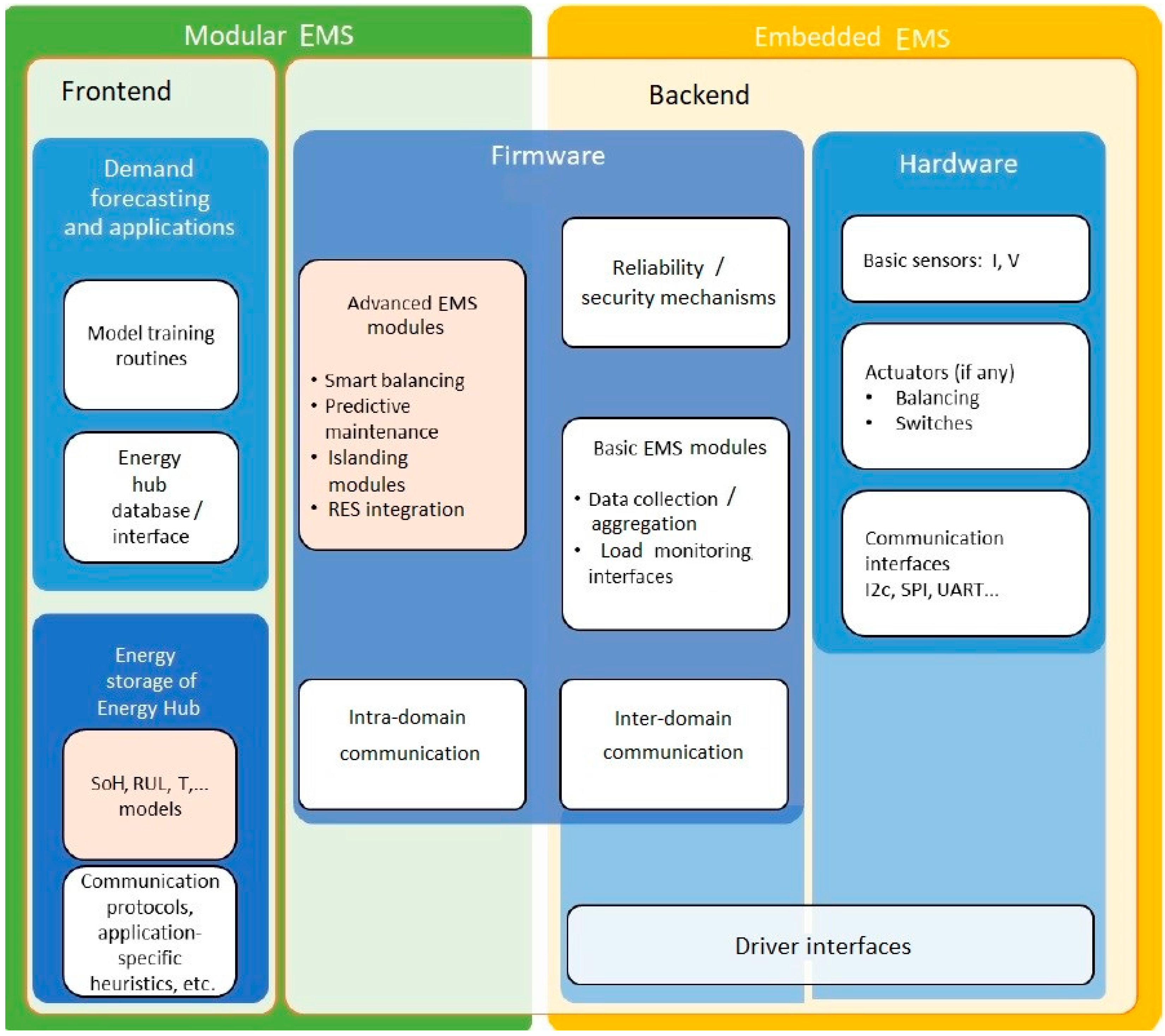
• An Energy Management System (EMS) for deploying the method in existing or newly formed SMs and providing an interface with utility operators.
• Validation in an existing Smart Microgrid (SM) of a typical Greek 17-bus low-voltage (LV) distribution network for calculating the Optimal Load Distribution, where results are compared through various operational scenarios and a sensitivity analysis aiming at criteria such as energy cost, total losses, and power generation distribution.

The rest of this article is organized as follows. Section 2 provides a brief overview of the microgrid and SM concepts as well as related work for the optimization aspects in EHs with MECs and EMS systems. Then, Section 3 presents the fundamental concept of EHs and describes the modeling principles (i.e., boundary conditions and constraints) as well as the EH system model. Afterward, Section 4 introduces the optimization problem in EHs for calculating the Optimal Power Flow (OPF) and the Optimal Load Distribution. The EH concept is applied in a typical Greek 17-bus LV distribution network within Section 5, allowing for the demonstration of different operational scenarios and the conducting of a sensitivity analysis to derive the Optimal Load Distribution. Finally, Section 6 provides a summary of the presented approach, concludes the article, and provides perspectives for future work.

2. Preliminaries

This section provides an overview of SMs by also focusing on the main elements they are composed of as well as related work on EHs, approaches similar to those presented in this article, and EMS systems.

2.1. Smart Microgrids Overview

Microgrids (MGs) are compact electric power systems composed of localized clusters of energy sources and loads. They usually operate in conjunction with the traditional centralized electrical grid, known as the macrogrid but also include the capability of detaching and operating autonomously depending on the specific physical or economic circumstances of the area where they are installed. Moreover, MGs operate by harnessing local energy sources (i.e., solar and wind power as well as energy storage), to provide dependable and secure electricity to local communities. Recently, they have attracted growing interest as an effective way to boost the resilience and dependability of the electricity grid.

The MG concept was initially introduced in the early 2000s, but it was not until 2007 that the concept gained significant attention in the literature [8]. Several studies have been conducted on the concept of MGs, showing promising results. For example, Guerrero et al. [9] demonstrated that MGs could enhance the stability and resilience of the electricity grid through the introduction of ancillary grid services such as voltage regulation and frequency control. Furthermore, Wang et al. [10] showed that MGs could reduce the overall cost of electricity, using local energy resources and avoiding the need for expensive transmission infrastructure. Further benefits of MGs include the integration of RESs i.e., solar and wind, which reduces the need for fossil fuel-based energy sources and consequently also greenhouse gas emissions [7,8,9,10,11].

SMs are a technological evolution of MGs, extending their basic operation by incorporating Internet of Things (IoT) technologies to optimize performance and efficiency as well as introduce automation mechanisms. SMs utilize advanced technologies such as sensors, control mechanisms, and communication systems to enhance the management of local energy resources and improve integration across different energy systems. Moreover, SM development specifically implies the use of automated observation, data acquisition, and analysis techniques within a single framework, which aids in the expansion of Multiple-Energy Systems (MESs) and EHs [12]. Fundamental elements of the SM are (1) the Advanced Metering Infrastructure (AMI) [13], enabling detailed energy usage monitoring as well as efficient energy management; (2) IoT-oriented communication protocols for controlling DG resources; and (3) optimization algorithms for balancing the electricity supply and load demand and providing feedback on the production/distribution infrastructure.

One of the earliest studies on SMs was conducted by Hatziargyriou et al. [8], who proposed the idea of an “intelligent MG” that uses advanced control algorithms to optimize the use of RES as well as enhance the dependability and effectiveness of the electricity grid. Specifically, the authors suggested that SMs could provide a range of benefits, including, apart from greenhouse gas emissions reduction, the improvement of energy security and the increased integration of RES. Additionally, Olivares et al. [14] demonstrated that SMs could enhance the management and synchronization among various energy systems, including electricity, heating, and cooling parts, hence leading to significant improvements in energy efficiency. Further work [15,16,17] has shown that SMs can lower the total electricity cost by maximizing the utilization of local energy resources and decreasing the reliance on costly transmission infrastructure.

2.2. Related Work

Over the later years, existing work on MECs and EHs has increased substantially. The EH concept and its different applications in households, commercial and industrial buildings, and agriculture with different energy consumption needs are presented in [18]. The strategies for modeling and optimizing EHs are presented in [19], which applies the mixed-integer linear programming (MILP) method to tackle challenges such as optimal dispatch or generation scheduling by resolving the associated optimization problems. Nevertheless, the problems are not applied in specific operational case studies and scenarios to derive solutions, but instead, a strategy and algorithms to solve them are proposed. More recent work [20] has tried to tackle the challenge of the absence in experimental scenarios and case studies in EHs. Specifically, the authors have formulated and verified a model within a commercial building, where the peak electricity usage reaches around 500 kW during summer weekdays and RES is also utilized (i.e., a PhotoVoltaic (PV) panel of 30 kW capacity).

Our approach focuses on optimizing the operation of EHs by calculating the Optimal Power Flow (OPF) and the Optimal Load Distribution of MECs. Further investigations into the Optimal Power Flow (OPF) of Multiple-Energy Carriers (MECs) are detailed in [5], where a universal dispatch optimization condition is derived. Additionally, the study in [21] employs a Monte Carlo method to analyze how EHs’ outputs respond to uncertain and fluctuating market prices. The authors in [22] introduce a detailed model for the long-term, multi-area, and multi-stage supply expansion planning of EHs, using a mixed-integer linear optimization to reduce both investment and operational costs. Moreover, a practical method employing quadratic programming, suitable for solving the real-time Economic Dispatch (ED) problem, is proposed in [23]. Other strategies to address the ED challenge include linear programming (depicted in [24]), weighted sum-based approaches in [25], and a constrained technique in [26]. A significant issue in modeling the ED for MECs and EHs lies in identifying global optimum solutions of the optimization model without imposing excessive computational loads.

The proposed approach is integrated into an EMS system, allowing it to (1) predict the actual load demand and (2) execute the optimization models inside it. The presence of EMS systems in SMs has been investigated both in terms of their electrical connections, operational functions, and modules as well as the employed communication technologies [27]. The main challenges when deploying EMS in SM however are linked to the heterogeneity of the components and the underlying technologies, in which case the EMS must act as a middleware for translating from one communication protocol and technology to another. Moreover, as EMS systems are deployed in embedded devices, there are also constraints in processing power and memory for predicting load demand and executing optimization models. A solution to these constraints can be obtained through the EMS interaction with cloud computing platforms; however, usually, utilities prefer to use local service platforms in their infrastructures and production sites to overcome data privacy and security challenges [28].

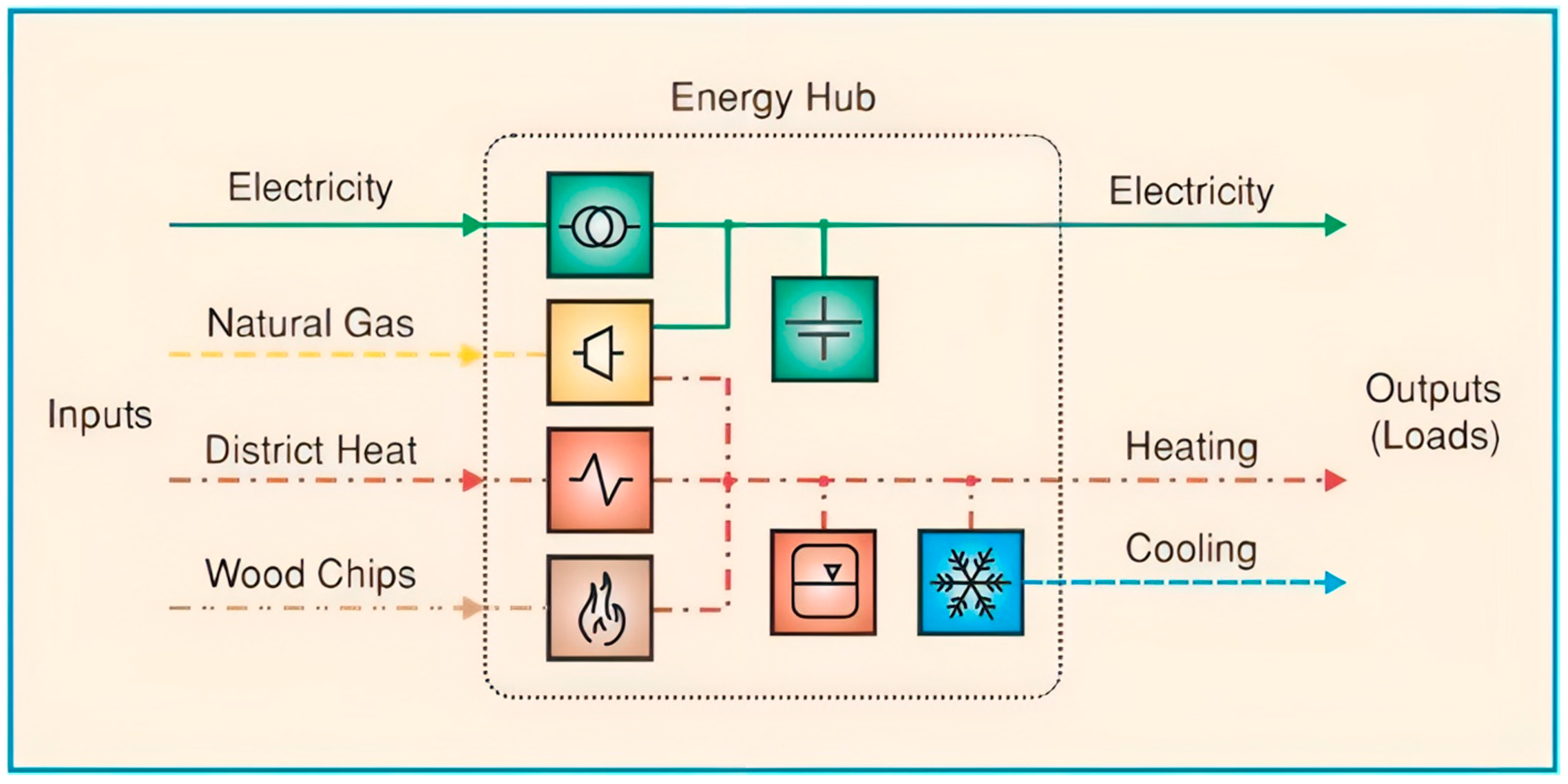
3. Modeling the Energy Carriers inside an Energy Hub

EHs incorporate different input energy sources for instance electricity and natural gas infrastructure in order to supply essential energy services including electricity, heating, and cooling as well as compressed air as output sources. To reach the output sources inside the EH, energy is transformed and managed using equipment such as CHP systems, transformers, power electronics, heat exchangers, compressors, converters, and further tools thoroughly explained in the literature [4,5,7]. Figure 1 presents a schematic of an EH with various energy inputs such as electricity, natural gas, district heat, and wood chips; it also highlights the hub’s capability to manage diverse types of energy in order to provide the output loads. Specifically, the EH receives the inputs and uses management, conversion, and storage functionalities for handling and optimizing multiple energy flows.

This is accomplished through transformation technologies such as electrical heaters, boilers, a power transformer, a small gas turbine, a heat exchanger, a battery, hot water storage, and cooling systems, each powered using different energy sources to produce the desired end-use energy forms. This showcases the EH’s role in delivering energy in the required forms for different usage scenarios, enhancing the collective effectiveness and adaptability of the energy system. Additionally, the outputs are directed towards specific applications: electricity is redistributed, while heating and cooling are delivered to satisfy thermal loads.

Several real installations can be modeled as EHs, such as cogeneration units, industrial facilities (e.g., steel mills and refineries), large buildings (e.g., airports, hospitals, and shopping centers), urban and rural areas, villages, cities, and individual electrical systems (e.g., airplanes, trains, and ships). EHs are powered using common energy carriers, including electrical energy, natural gas, and heat. Notably, hydrogen, biomass/biogas, geothermal energy, and household waste are also particularly interesting today. Conversely, all the aforementioned energy carriers can be supplied as outputs directly from the EH if they are not converted into other forms. Furthermore, energy can be transformed for cooling, heating, or producing compressed air or steam. The EH concept provides significant flexibility in system modeling, allowing the introduction of various energy carriers and products [6,12].

The existing energy infrastructure can be viewed as a network of interconnected EHs, where the diversity achieved in the supply results in the following advantages: increased reliability, enhanced load supply flexibility, optimization possibilities, and synergy benefits.

3.1. Modeling Principles

An important aspect of the EH model relates to the boundary conditions under which switching between gas and electricity occurs. These conditions first and foremost are linked to the accurate prediction of the electrical and thermal energy demand for the area where the EH is operational. Depending on the seasonal and temperature aspects in a specific area, the needs may vary; for instance, in colder or warmer seasons and areas, higher volumes of gas are required for heating or cooling, respectively. Likewise, in peak load demand, electricity is required more than gas. Furthermore, the conversion from one energy source to another affects the performance of the developed model as different types of devices as inverters or even transformers may be used to perform such conversion and based on their specifications the energy amount that is introduced in them is usually not the same as they produce since there are losses during the conversion. In practice, achieving above an 80% conversion rate is extremely challenging; hence, the devices used for the conversion are significant as a boundary condition for the proposed model.

Moreover, the market prices of gas and electricity serve as another distinct boundary condition since changes in them may occur at any moment. Specifically, switching from gas to electricity when electricity prices drop below a certain threshold might lead to significant costs as well as electricity bill reduction. Additionally, a boundary condition that is of equal importance is the presence of RESs and energy storage (mostly linked to batteries) mechanisms inside the EH, which can be used as an additional energy supply source to cope with peak load demand, instead of switching energy from gas to electricity. Finally, further conditions exist linked to regulatory compliance, following incentives that are given by governmental entities to switch towards cleaner energy sources, to facilitate the reduction in atmospheric pollutants. Nevertheless, these conditions are not considered within the scope of this article as they are specific for each country and area.

Based on the described boundary conditions, the reader may reflect that there are certain constraints when modeling an EH and upon the model’s use for calculating the Optimal Load Distribution, as detailed in Section 4. Initially, an accurate energy demand forecast is required, which depends on the amount of gathered historical energy consumption and temperature data for model training and the ML model selection and its associated learning/prediction mechanisms. Afterwards, the availability of gas and electricity prices requires integration with energy market platforms, in order to retrieve real-time price data. Such integration is considered very complex as these platforms are usually proprietary and access to them is restricted only to the involved entities in the electricity and gas production market. Given the described boundary conditions and constraints, in the following part, we present the EH system model.

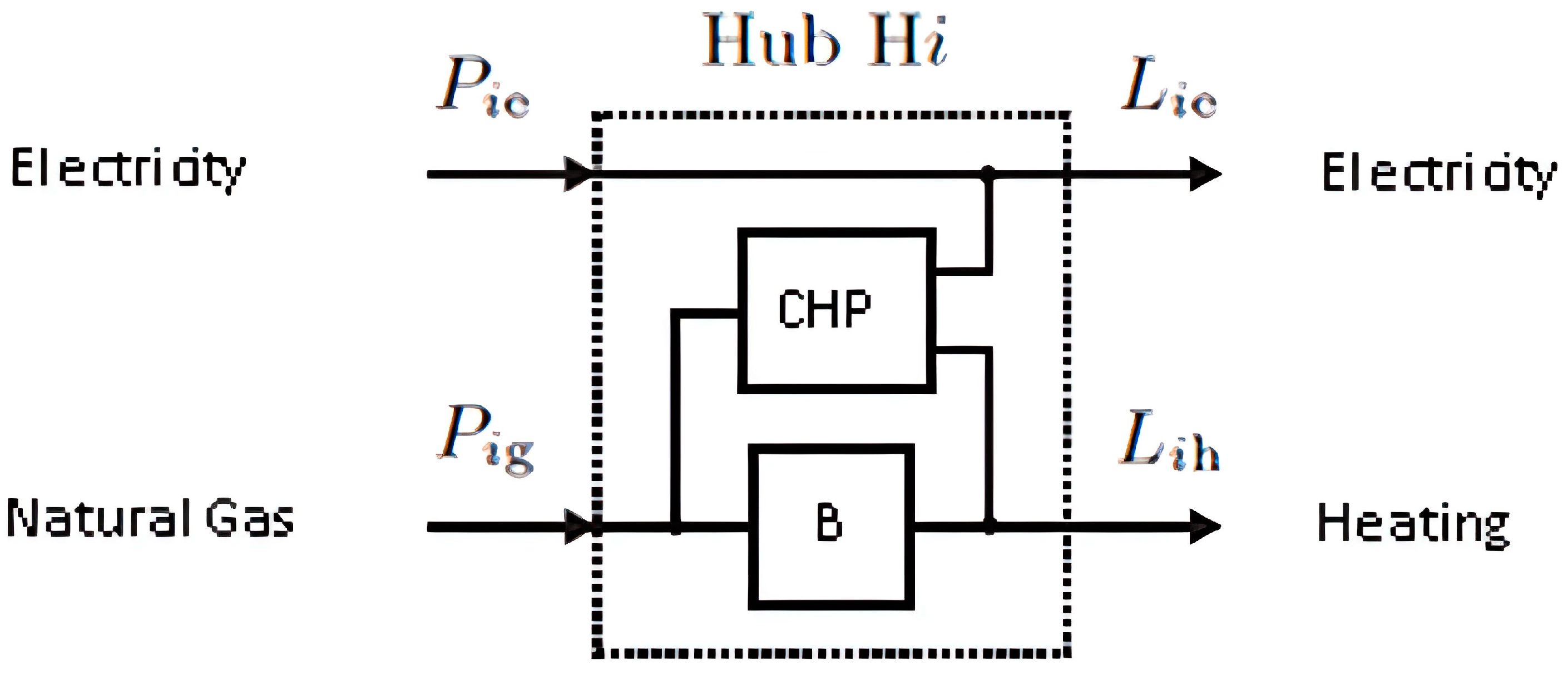
3.2. Energy Hub System Model

If we consider the vectors P and L as the inputs and outputs of power for an EH, respectively, the EH fundamental equation, based on [5], is

$$\left[\begin{array}{c}{\mathrm{L}}_{\mathsf{\alpha }}\\ {\mathrm{L}}_{\mathsf{\beta }}\\ \begin{array}{c}⋮\\ {\mathrm{L}}_{\mathsf{\omega }}\end{array}\end{array}\right]=\left[\begin{array}{ccc}{\mathrm{c}}_{\mathsf{\alpha }\mathsf{\alpha }}& \cdots & {\mathrm{c}}_{\mathsf{\omega }\mathsf{\alpha }}\\ ⋮& \ddots & ⋮\\ {\mathrm{c}}_{\mathsf{\alpha }\mathsf{\omega }}& \cdots & {\mathrm{c}}_{\mathsf{\omega }\mathsf{\omega }}\end{array}\right] \left[\begin{array}{c}{\mathrm{P}}_{\mathsf{\alpha }}\\ {\mathrm{P}}_{\mathsf{\beta }}\\ \begin{array}{c}⋮\\ {\mathrm{P}}_{\mathsf{\omega }}\end{array}\end{array}\right] \mathrm{or} \mathrm{L}=\mathrm{CP}$$

(1)

$$0 \le {\mathrm{c}}_{\mathsf{\alpha }\mathsf{\beta }} \le 1 \forall \mathsf{\alpha }, \mathsf{\beta } \in \mathsf{\epsilon } (\mathrm{The} \mathrm{energy} \mathrm{carriers} \mathrm{set})$$

(2)

$$0 \le {{\displaystyle \sum }}_{\mathsf{\beta }ϵ\mathsf{\epsilon }}{\mathrm{c}}_{\mathsf{\alpha }\mathsf{\beta }} \le 1 \forall \mathsf{\alpha } \in \mathsf{\epsilon }$$

(3)

The C matrix is referred to as the coupling matrix of the converters. Each element of C, denoted as cαβ, is a coupling factor between a specific input and output, constrained between 0 and 1, indicating the portion of input power converted to output power (Equation (2)). These coupling factors reflect the system’s capability to transform, store, or distribute energy from various sources to different loads, but they are not directly indicative of energy efficiency. A further EH equation related to cαβ is Equation (3), denoting that for any input energy source α, across all outputs β, it does not exceed 1.

It should also be noted that, in general, the matrix C is not invertible, and, thus, Equation (1) represents a system with parametrically infinite solutions, revealing the degrees of freedom of the system, hence allowing optimization to be applicable. The non-invertibility of C implies the system can have multiple solutions, highlighting the importance of optimization to identify the most efficient or cost-effective operational strategy. The constraints ensure that the conversion rates are realistic, bounded, and applicable to all energy carriers within the system. Moreover, an important distinction is that in systems with multiple inputs and outputs, unlike single-input–single-output converters, the coupling factors of the converters are generally not equivalent to their energy efficiencies.

Furthermore, in the case of storage integration into an EH, the following equations focus on how stored and input powers are related through a storage coupling matrix and its impact on the Energy Hub’s output flows. Specifically, if M is the vector for stored output powers and Q is the corresponding vector for input powers, then the following equation holds [6]:

$${\mathbf{L}}_{ }=\mathbf{C} \left[\mathbf{P}-\mathbf{Q}\right]-\mathbf{M}=\mathbf{C} \mathbf{P}-{(\mathbf{M}+}_{ }\mathbf{CQ})=\mathbf{C} \mathbf{P}-{\mathbf{M}}^{\mathbf{eq}}$$

(4)

This equation formalizes the relationship between output power (L), input power (P), stored power (Q), and the equivalent stored output power (${\mathrm{M}}^{\mathrm{eq}}$), incorporating the storage effect into the energy balance. It particularly highlights the subtraction of the equivalent stored power from the product of matrix C and input power to obtain the final output power, emphasizing the role of storage in energy distribution. Additionally, the equivalent stored power (${\mathrm{M}}^{\mathrm{eq}}$) in terms of the storage coupling matrix (S) and the rate of change of stored energies (Ė) is defined by Equation (5), which links the storage system’s dynamics directly to its contribution to the EH output flows. Equivalently, it relates all derivatives of stored energies (Ė) to their corresponding output flows.

$$\left[\begin{array}{c}{\mathrm{M}}_{\mathsf{\alpha }}^{\mathrm{eq}}\\ {\mathrm{M}}_{\mathsf{\beta }}^{\mathrm{eq}}\\ \begin{array}{c}⋮\\ {\mathrm{M}}_{\mathsf{\omega }}^{\mathrm{eq}}\end{array}\end{array}\right]=\left[\begin{array}{ccc}{\mathrm{s}}_{\mathsf{\alpha }\mathsf{\alpha }}& \cdots & {\mathrm{s}}_{\mathsf{\omega }\mathsf{\alpha }}\\ ⋮& \ddots & ⋮\\ {\mathrm{s}}_{\mathsf{\alpha }\mathsf{\omega }}& \cdots & {\mathrm{s}}_{\mathsf{\omega }\mathsf{\omega }}\end{array}\right] \left[\begin{array}{c}{\dot{\mathrm{E}}}_{\mathsf{\alpha }}\\ {\dot{\mathrm{E}}}_{\mathsf{\beta }}\\ \begin{array}{c}⋮\\ {\dot{\mathrm{E}}}_{\mathsf{\omega }}\end{array}\end{array}\right] \mathrm{or} M^{eq}=S\dot{\mathbf{E}}$$

(5)

Ultimately, drawing from Equations (1), (4), and (5), the flows through an EH are described as follows:

$${\mathbf{L}}_{ }=\mathbf{C} \mathbf{P}-\mathbf{S}\dot{\mathbf{E}}=\left[ \mathbf{C}- \mathbf{S} \right]\left[ \begin{array}{c}\mathbf{P} \\ \dot{\mathbf{E}} \end{array}\right]$$

(6)

Specifically, this equation simplifies the system’s overall energy flow equation, showing how output power is derived from input power minus the product of the storage coupling matrix and the rate of change in stored energy. This equation encapsulates the integrated model of a hybrid EH, including transport, conversion, and storage, and highlights the underdetermined nature of the system, which allows for multiple input configurations to achieve a desired output, thus increasing the system’s operational flexibility.

Evidently, the above equations are underdetermined, allowing for multiple input vectors that satisfy a given output, thereby providing the possibility to choose the optimal input based on the specified criteria. On the other hand, it becomes apparent that the introduction of storage units enhances the operational flexibility of the energy distributor. Furthermore, the losses within the EH are reflected in the following equation:

$$\mathsf{\lambda }={{\displaystyle \sum }}_{\mathrm{k}\in \mathsf{\epsilon }}{\mathrm{P}}_{\mathrm{input},\mathrm{k}}\pm {{\displaystyle \sum }}_{\mathrm{k}\in \mathsf{\epsilon }}{\mathrm{P}}_{\mathrm{total} \mathrm{storage},\mathrm{k}}+{{\displaystyle \sum }}_{\mathrm{k}\in \mathsf{\epsilon }}{\mathrm{P}}_{\mathrm{standby},\mathrm{k}}-{{\displaystyle \sum }}_{\mathrm{k}\in \mathsf{\epsilon }}{\mathrm{P}}_{\mathrm{output},\mathrm{k}}$$

(7)

Specifically, this equation reflects that the total losses (λ) are determined by the sum of the input power (Pinput), the net power of storage units that can either be added or subtracted based on the charging or discharging state of the storage (Ptotal storage), the standby unit power (Pstandby), and the output power (Poutput). The equation accounts for the directionality of storage effects, where charging storage will appear to increase losses (due to energy being diverted into storage) and discharging will reduce apparent losses (as energy is released from storage). Standby losses are also included, reflecting the energy consumed when systems are on standby mode and not actively contributing to the output power. Thus, the “−” corresponds to the case of energy storage, and the “+” is when energy is injected back into the EH. Furthermore, it shall be noted that a storage unit in an EH would result in an apparent reduction or increase in its losses, depending on whether it is discharged or charged during a specific period.

All the previous equations allow for the modeling of functions such as energy transport, storage, and conversion within a connected network of energy distributors. Ultimately, the conversion and storage of energy are determined by the coupling matrices of the converters, C_i, and the storage coupling matrix, S_i, of each EH_i, i∈H, respectively. Thus, the energy flow in each EH is described according to Equation (8):

$${\mathbf{L}}_{ }=\left[{ \mathbf{C}}_{\mathbf{i}}-{ \mathbf{S}}_{\mathbf{i}} \right]\left[ \begin{array}{c}{\mathbf{P}}_{\mathbf{i}} \\ {\dot{\mathbf{E}}}_{\mathbf{i}}\end{array}\right] \forall \mathrm{i} \in \mathrm{H}$$

(8)

Overall, this equation includes the coupling matrices for converters (C_i) and storage (S_i), along with the vectors of input power (P_i) and stored energy (E_i) for each EH. This relationship applies to every EH within the set H using the notation ∀i ∈ H in Equation (8). Moreover, the equation captures how the input power and energy stored within each EH are transformed and managed to meet the demand, which is represented by the vector L. Finally, for the interconnection between EHs and the network, we consider that the inputs and outputs of the EHs represent power injections into various nodes.

4. Proposed Approach for Optimal Load Distribution

Many optimization challenges with several energy carriers correspond to well-known and common problems, such as (1) Economic Dispatch (ED), (2) Optimal Power Flow (OPF), and (3) Optimal Facility Siting [29,30]. Typically, the goal is to minimize the operational energy cost of the examined system, reduce emissions of environmentally harmful gases, or simultaneously optimize both economic and environmental aspects through “Economic and Environmental Dispatch”. Additionally, when optimizing a system, the convexity or non-convexity of the solution space and sensitivity analysis of the objective function with respect to optimization variables are of particular interest [31,32,33]. In this section, we first present the problem of OPF in an electrical network (Section 4.1) and subsequently formulate the generic optimization problem involving MECs within an SM (Section 4.2).

Finally, Section 4.3 also includes an overview of an Energy Management System (EMS), which is very important for our approach. Specifically, prior to the use of any optimization method, a preliminary step has to be followed for forecasting the energy demand, which serves as an entry point for our approach. The reason we have included in the last part of this section is to demonstrate the applicability and deployment of our approach through an EMS that provides energy demand predictions, executes the models, and performs required calibrations to ensure the EH continuous availability and satisfaction of the energy demand–response equilibrium.

In detail, energy demand is forecasted using historical energy consumption and temperature data to train Machine Learning (ML) models that can be used to derive accurate predictions as the Temporal Fusion Transformer (TFT) model that is detailed in [34]. The TFT includes the Transformer and the Temporal Fusion Decoder (TFD) modules, where the former captures the long-term dependencies in energy consumption data and the latter uses the Long Short-Term Memory Network (LSTM) layers to learn these dependencies. The ML models are thoroughly explained in Section 4.3 within the EMS system.

4.1. Optimal Power Flow Computation

The OPF is a critical issue in managing power systems. It was initially introduced by Carpentier [35] as a nonlinear programming problem, extending the Economic Dispatch (ED) problem. Since its introduction, it has become a principal topic in nonlinear optimization.

OPF is a constant nonlinear optimization problem that determines an optimal set of variables based on network conditions, load information, and system parameters. It aims to minimize specific targets, such as generation costs or losses in power transmission, while adhering to various constraints. The objective is to determine the optimal state variables, X, to reduce an objective function, F(X), which could reflect either the costs of power generation or the actual power losses. The formulation of the OPF problem is outlined as follows:

$$minimize \mathit{F}\left(\mathit{X}\right)$$

$$subject to \left\{\begin{array}{c}{g}_i\left(X\right)=0, 1\le i\le m\\ h_j\left(X\right)\le 0, 1\le j\le q\\ X^{min}\le X\le X^{max}\end{array}\right.$$

(9)

where $X\in {ℝ}^n$, $n>m$, represents the state variables vector, including voltage magnitude and phase angles. $F : {ℝ}^n\to ℝ$ indicates the objective function reflecting system performance and that specifically focuses on real power losses in transmission or costs associated with generation. The constraints $g_i : {ℝ}^n\to ℝ$ are based on the power flow equations and are derived from the principle of energy conservation at all system buses. The functions $h_j : {ℝ}^n\to ℝ$, $q<m$ outline the operational limitations for power flow within the transmission lines and bus systems. Moreover, $X^{min}\le X\le X^{max}$ indicates the vector inequality, which (1) specifies component-wise inequalities and (2) represents system constraints on transmission lines, buses, and other operational parameters. Furthermore, the X variables include voltage levels and phase shifts at different bus locations within the system, reflecting the state of the electrical network. Additionally, the functional constraints ensure that the solution adheres to the physical and power system technical constraints, including limits on generation capacities and voltage thresholds. Finally, the load flow equations (gi) based on [36,37] are as follows:

$${\mathrm{P}}_{\mathrm{Gi}}-{\mathrm{P}}_{\mathrm{Di}}={ \mathrm{V}}_{\mathrm{i}}·{{\displaystyle \sum }}_{\mathrm{j}=1}^{\mathrm{n}}{\mathrm{V}}_{\mathrm{j}}·\left[{\mathrm{G}}_{\mathrm{ij}}\cos \left({\mathsf{\delta }}_{\mathrm{i}}-{\mathsf{\delta }}_{\mathrm{j}}\right)+{\mathrm{B}}_{\mathrm{ij}}\sin \left({\mathsf{\delta }}_{\mathrm{i}}-{\mathsf{\delta }}_{\mathrm{j}}\right)\right]$$

(10)

$${\mathrm{Q}}_{\mathrm{Gi}}-{\mathrm{Q}}_{\mathrm{Di}}={ \mathrm{V}}_{\mathrm{i}}·{{\displaystyle \sum }}_{\mathrm{j}=1}^{\mathrm{n}}{\mathrm{V}}_{\mathrm{j}}·\left[{\mathrm{G}}_{\mathrm{ij}}\sin \left({\mathsf{\delta }}_{\mathrm{i}}-{\mathsf{\delta }}_{\mathrm{j}}\right)-{\mathrm{B}}_{\mathrm{ij}}\cos \left({\mathsf{\delta }}_{\mathrm{i}}-{\mathsf{\delta }}_{\mathrm{j}}\right)\right]$$

(11)

In these equations, P_G and P_L denote the active power generation and load demand from the different EH energy sources. In detail, the active power depicts the component of electrical power that measures “real” power consumed by electrical devices in AC LV networks. Similarly, Q_G and Q_L denote the reactive power generation and load demand from the different EH energy sources. Reactive power indicates the electrical power component oscillating between source and load, thus enabling the establishment of electric and magnetic fields necessary for the operation of certain types of equipment as motors and transformers.

Hence, Equation (10) defines the balance of real power at node i (P_Gi − P_Di), where P_Gi is the produced real power and P_Di is the real power that is required as a part of the demand at node i. The equation sums the product of voltage at node i (V_i) and voltage at node j (V_j) with the network parameters Gij and Bij, which reflect the electrical conductivity as well as the inductive/capacitive reactance between nodes i and j. Furthermore, the equation includes the cosine and sine of the difference in angle between nodes i and j (i.e., δi − δj), for all nodes j connected to node i.

Furthermore, Equation (11) defines the reactive power balance at node i (Q_Gi − Q_Di), where Q_Gi is the produced reactive power and Q_Di is the reactive power that is required as a part of the demand at node i. It has a similar structure to Equation (10) but with the sine and cosine functions swapped, reflecting the orthogonal relationship between real and reactive power in Alternate Current (AC) systems.

Numerous algorithmic methods have been explored over time, seeking to provide efficiency in OPF computation [29,30]. Specifically, several constrained optimization approaches, such as penalty functions, Lagrange Multipliers, sequential quadratic programming, and gradient and Newton methods for tackling unconstrained optimization, have risen to prominence as the key nonlinear programming (NLP) algorithms for resolving AC OPF challenges. Among the existing work, the methods that are more widely adopted are the Lagrange Multiplier, Particle Swarm Optimization (PSO), and Harmony Search (HS). Initially, the Lagrange Multiplier operates by converting a constrained optimization problem into an unconstrained one by employing Lagrange Multipliers. Moreover, the objective function of this method seeks to minimize the overall generation cost while adhering to constraints such as power balance. These constraints are combined into a single Lagrangian function, aiming to minimize the total generation cost and maximize the system’s efficiency. Overall, the Lagrange Multiplier is useful in systems where the constraints can be clearly defined and are differentiable and integrable into the objective function in order to offer a precise analytical solution. Due to their analytical nature, the performance and computational resources that are required rely heavily on (a) the problem being differentiable and (b) the existence of a closed-form solution.

Another well-known method for OPF computation is PSO, which is a metaheuristic algorithm identifying optimal solutions in complex, high-dimensional spaces without the need for gradient information or being too sensitive to the problem’s initial conditions. PSO lists multiple solutions called particles, where each one adjusts its position based on data inputs and the interaction with neighboring particles, moving towards the best-found positions. This process iterates until a convergence on an optimal or near-optimal solution. PSO is usually employed in optimization problems with nonlinear and non-convex characteristics as well as in large and complex scenarios and input datasets.

Finally, HS is an algorithm for OPF computation performed by efficiently searching for the global optimum with a balance between exploration and exploitation. Each solution vector in HS is considered a “harmony”, inspired by the music field. Then, the algorithm iteratively tries to improve the harmony by considering various combinations of decision variables and is especially applied in situations where the problem landscape is irregular i.e., rugged or discontinuous.

Upon comparing the three well-known methods for OPF computation, while the Lagrange Multiplier provides an analytical technique that offers precision in the solution, the PSO and HS methods allow researchers to tackle complex, nonlinear, and dynamic problems where traditional analytical methods may have performance issues and long computational times. Nevertheless, the selection of the best-suited method for OPF computation depends on (1) the constraints of the problem where optimization shall be applied, (2) the complexity and dimensionality of the solution space, (3) the desired precision and accuracy, and (4) computational resources that are available for executing the model with the selected method until a candidate solution is identified. Within the proposed approach, we have employed all three algorithms, i.e., Lagrange Multiplier, PSO, and HS, to solve the problem of Optimal Load Distribution in the case study of Section 5, where multiple operational scenarios are examined. Specifically, the studied scenarios have a different problem focus (i.e., both analytical with the need for a precise solution as in the case of a typical 17-bus LV distribution network as well as more complex and dynamic solutions when integrating into this network RESs, CHP, and EVs).

4.2. Optimal Load Distribution of Energy Carriers with Multiple Energy Sources

The optimization analysis of load flows in a network of interconnected EHs with multiple energy sources involves finding the best operational strategy for the entire system and its overall condition and encompassing the transfer and conversion of multiple energy sources while adhering to the system’s safety constraints [5,8].

The objective function that shall be minimized (usually operational cost minimization) will depend on the utilization of EH converters P_i, stored energies Ε_i, and network load flows for each network flow element F_α, where i$\in$H and $\mathsf{\alpha }\in \mathsf{\epsilon }$. A set of inequalities limits the solution space of the optimization problem. Specifically, the equality constraints arise from the load flow equations of EHs and the network, while the inequality constraints pertain to the input limits of EH converters P_i as well as the network flows F_α. The minimum and maximum limits of all these elements are denoted as ${\underset{\_}{\mathbf{P}}}_{\mathrm{i}}$, ${\overline{\mathbf{P}}}_{\mathrm{i}}$ and ${\underset{\_}{\mathbf{F}}}_{\mathsf{\alpha }}$, ${\overline{\mathbf{F}}}_{\mathsf{\alpha }}$, respectively. Additionally, inequality constraints are associated with energy storage (E). On the input side, where energy sources are stored ρ$\in$ε, the corresponding limits are ${\underset{\_}{\mathrm{Q}}}_{\mathsf{\rho }}$ and ${\overline{\mathrm{Q}}}_{\mathsf{\rho }}$. On the output side, where energy carriers are stored σ$\in$ε, the respective bounds are ${\underset{\_}{\mathsf{{\rm M}}}}_{\mathsf{\sigma }}$ and ${\overline{\mathsf{{\rm M}}}}_{\mathsf{\sigma }}$. Typically, optimization spans multiple time periods t; thus, all referenced quantities are time-dependent. Ultimately, the problem of OPF with multiple energy sources constitutes a nonlinear programming challenge and is mathematically formulated as follows:

$$\mathrm{Minimization} \mathrm{of} \mathrm{Op}.\mathrm{C} \mathrm{O}p.\mathrm{C}={\sum }_{\mathrm{t}=1}^{\mathrm{Nt}}\mathsf{O}\mathrm{p}{.\mathrm{C}}^{\mathrm{t}}{(\mathbf{P}}_{\mathrm{i}}^{\mathrm{t}}{ , \mathbf{E}}_{\mathrm{i}}^{\mathrm{t}}{ , \mathbf{F}}_{\mathsf{\alpha }}^{\mathrm{t}} , \mathbf{X} )$$

(12)

$$\mathrm{s}.{\mathrm{t} \mathbf{L}}_{\mathrm{i}}^{\mathrm{t}}-{\mathbf{C}}_{\mathrm{i}}^{\mathrm{t}}·{\mathbf{P}}_{\mathrm{i}}^{\mathrm{t}}{+\mathbf{M}}_{\mathrm{i}}^{\mathrm{eq} \mathrm{t}}=0$$

(13)

$$M^{\mathrm{eq} \mathrm{t}}=S^{\mathrm{t}} {\dot{\mathbf{E}}}^{\mathrm{t}}=S^{\mathrm{t}} \left(E^{\mathrm{t}}-E^{\left(\mathrm{t}-1\right)}+E^{\mathrm{stanby}}\right)$$

(14)

$${\mathbf{G}}_{\mathsf{\alpha }}^{\mathrm{t}}=0$$

(15)

$${\mathit{g}}_{\mathit{k}}\left(\mathit{X}\right)=0$$

(16)

$${\underset{\_}{\mathbf{P}}}_{\mathrm{i}}^{\mathrm{t}} \le { \mathbf{P}}_{\mathrm{i}}^{\mathrm{t}} \le {\overline{\mathbf{P}}}_{\mathrm{i}}^{\mathrm{t}}$$

(17)

$${\underset{\_}{\mathbf{Q}}}_{\mathrm{i}\mathsf{\rho }} \le { \mathbf{Q}}_{\mathrm{i}\mathsf{\rho }}^{\mathrm{t}} \le {\overline{\mathbf{Q}}}_{\mathrm{i}\mathsf{\rho }}$$

(18)

$${\underset{\_}{\mathbf{M}}}_{\mathrm{i}\mathsf{\sigma }} \le { \mathbf{M}}_{\mathrm{i}\mathsf{\sigma }}^{\mathrm{t}} \le {\overline{\mathbf{M}}}_{\mathrm{i}\mathsf{\sigma }}$$

(19)

$${\underset{\_}{\mathbf{E}}}_{\mathrm{i}}^{\mathrm{t}} \le { \mathbf{E}}_{\mathrm{i}}^{\mathrm{t}} \le {\overline{\mathbf{E}}}_{\mathrm{i}}^{\mathrm{t}}$$

(20)

$${\underset{\_}{\mathbf{F}}}_{\mathsf{\alpha }}^{\mathrm{t}} \le { \mathbf{F}}_{\mathsf{\alpha }}^{\mathrm{t}} \le {\overline{\mathbf{F}}}_{\mathsf{\alpha }}^{\mathrm{t}}$$

(21)

$$X^{min}\le X\le X^{max}$$

(22)

$${\mathit{h}}_{\mathit{j}}\left(\mathit{X}\right)\le 0$$

(23)

where $\mathrm{t} \in \left\{ 1, 2,\dots , \mathrm{Nt} \right\}$; i$\in$H; $\mathsf{\alpha }, \mathsf{\rho }, \mathsf{\sigma } \in \mathsf{\epsilon }$; and 1 ≤ k ≤ m. The EHs indicated by ρ are held at the input and the carriers are listed as σ at the output, with ρ ≠ σ.

The mathematical Equations (12)–(23) present different aspects that are followed for the optimization. Initially, Equation (12) reflects the overall minimization objective that is linked to the operational costs, considering converter utilization, stored energies, and network load flows, to be minimized over time. Then, Equation (13) presents the balance condition for ensuring that demand is met. Hence, the combination of load demands, converter outputs, and equivalent stored energy in each EH must equal zero. Furthermore, Equation (14) defines the change in stored energy, by taking the standby losses into consideration. Afterward, Equations (15) and (16) ensure that the power flows and network constraints, respectively, are satisfied. The network constraints may include voltage limits at different nodes, maximum and minimum power flow limits on transmission lines, and phase angle differences to maintain system stability and reliability. They should always be considered in the optimization model to ensure the physical and safety limitations of the electrical network are adhered to, thereby preventing equipment damage and ensuring a reliable supply of electricity.

Finally, Equations (17)–(24) define the bounds on the matrices for identifying solutions for the model. Specifically, Equation (17) defines the limits on converter input powers, Equation (18) defines the limits on the stored energy inputs, and Equation (19) defines the limits on the stored energy outputs. Additionally, Equation (20) defines the limits for the energy levels in terms of storage and Equation (21) defines the limits on the network flows along with general variable bounds in Equation (22) and inequality constraints in Equation (23).

Alternatively, decentralized control can be utilized. In this case, the optimization problem is divided into as many coupled sub-problems as the considered regions instead of being consolidated as in the aforementioned equations. Similar problems can be formulated for the optimal coupling of EHs or optimal designs.

The optimization problem generally involves nonlinear constraints, and, thus, the solution space is not convex. Consequently, the numerical methods used for the solution do not guarantee finding the global minimum. Conversely, when the objective function is convex and the constraints are either linear or have been linearized, then achieving a global minimum is possible. In such a scenario, the Karush–Kuhn–Tucker (KKT) conditions are both necessary and sufficient for identifying the global minimum in optimization [31]. As an outcome, the general optimization requirement for linear distributors can be formulated as follows:

Ψ = Λ C

(24)

Specifically, in Equation (24), Ψ and Λ are vectors composed of the boundary costs at the energy distributor input and output, respectively, and C is a matrix related to the conversion or distribution efficiencies, costs, or coefficients that link inputs to outputs within the energy distributor system. Specifically, Ψ represents the costs associated with the inputs into the energy distributor, such as financial costs; energy losses; and carbon emissions. Each element of Ψ corresponds to a different input source or resource. Similarly, it reflects the costs associated with the outputs from the energy distributor as power, gas, heat, and storage. Finally, C represents the conversion between inputs and outputs as well as the distribution coefficients or cost factors associated with transforming or transporting energy from its main source to its usage.

4.3. Energy Management System Integration within the Energy Hub

Energy management for the proposed approach is performed through the presence of an EMS. The EMS coordinates energy generation, storage, and consumption across the MEC sources of the EH as well as their individual loads. Moreover, it integrates load demand-forecasting modules using ML models trained with historical consumption data for predicting energy demand patterns, enabling proactive adjustments to energy supply and consumption strategies [34]. Additionally, the EMS can also be integrated with an SM, allowing the EH to (1) operate independently from the main grid during outages and (2) have cyber-resilience in the presence of cyber-attacks [38]. Utilities usually refer to this operation using the term “islanding”, inferred by the islands that often have isolated SM networks, communicating with the mainland through underwater pipes whenever possible.

The EMS is responsible for switching between MECs primarily based on the forecasted energy demand in the area where the EH is deployed i.e., considering both electricity and gas demand based on the temperature conditions. To this end, the prediction accuracy of the ML models in the EMS is of vital importance, as the produced energy in the EH shall be equal to the forecasted demand in order to satisfy the demand/response equilibrium. Moreover, to satisfy this demand and allow switching between different MECs, additional criteria are employed, centered around economic, environmental, and operational factors. Specifically, the criteria are (1) the availability of Renewable Energy from wind turbines as well as PV panels, where electricity is produced from natural sources without any actual cost; (2) relative costs of electricity and gas, which are linked to their market price (i.e., electricity prices are usually significantly higher than gas in peak demand periods); (3) the capacity of the energy storage solutions that are available in the EH; and, finally, (4) the conversion performance using inverters for transforming energy in different forms, including gas and electricity, depending on the real-time needs.

As denoted in the Section 4 introduction, forecasting is based on the TFT transformer model [30]. The model uses LSTM for learning long-term dependencies in energy consumption, indoor and outdoor temperature, indoor and outdoor humidity, and global horizontal radiation. The derived prediction accuracy from the model depends on the timespan of data gathering and a recommended data volume spans over the course of a year for each building or household, in order to allow for the observing of adequate seasonal and temperature variations and for the training of the model. In a typical household or building, the electrical energy consumption data are gathered from smart meter devices and result approximately in a 5,256,000 total entry size, which in turn requires 250 MB of data storage for each one (i.e., given 50 bytes of storage per entry as detailed in [34]).

In terms of energy demand prediction, the model is able to achieve very good results, especially through edge-based deployment [34]. These results serve as a base for deriving a Short-Term Load Forecast that serves as a base for the EMS system. Furthermore, such a basis can be used for planning ahead on the overall energy to be produced through the EH MEC carriers. Nevertheless, a current model restriction lies in the prediction accuracy of thermal energy demand due to the lack of sufficient data on the thermal load. Specifically, as also denoted in Section 5, the thermal load data that are used are generic based on the existing district heating network installed in northern Greece [34] and not specific to the building/household. Usually, such data are derived in substantially higher quantities using smart meters for gas consumption. However, in our setup, we could only install electrical and not gas-oriented smart meters due to imposed restrictions in the deployed households. Additionally, existing fine-grained datasets [39] could not be used, due to the difference in the climate conditions in the area where they are gathered from.

The EMS system architecture is depicted in Figure 2. This architectural view splits the EMS into a modular and an embedded part. The modular part includes the frontend of the EMS, which is the main interaction point of the operators with the EH. It consists of the ML models for load demand forecasting, the EH database with the MECs, and the energy storage interface of the EH with dedicated models for calculating important battery-oriented indicators such as the State of Health (SoH), the Remaining Useful Life (RUL), and the operating temperature. Furthermore, the embedded EMS part includes the EMS backend, which has all the reliability and security mechanisms, optimization modules, algorithms, and the interface with sensors/actuators for gathering environmental (e.g., temperature) or energy (i.e., current and voltage) inputs. This is accomplished using intra-domain and inter-domain communication modules to facilitate the data exchange within the EH and with further EHs, respectively. The backend is composed of the firmware and the hardware where it is deployed, which interact using the driver interfaces and libraries of the EMS.

Finally, the EMS provides a dashboard within the frontend part of the architecture. The dashboard serves as a visualization tool for operators and users, allowing them to monitor energy flows and system performance.

5. Case Study: Energy Hubs in a 17-Bus LV Distribution Network

The proposed method is applied in this section to investigate an optimization problem of operational cost in an SM that incorporates EHs, through five (5) distinct operational scenarios and a corresponding sensitivity analysis.

Figure 3 depicts an SM in terms of a 17-bus distribution network in LV, which is built to exhibit similar behavior to a typical Greek LV network. In this SM, the network’s feeders are equipped with various DGs, including one Micro Turbine (MT), one Fuel Cell (FC), a directly coupled wind turbine (WT), several micro-Combined Heat and Power units (mCHPs), and numerous PVs. Initially, the WT (point 1 in the LV network) converts kinetic energy from wind into electrical energy. Then, PVs with different characteristics and capacity (in kW) are connected at point 4 (PV 2 .. 5 in Figure 3) and point 5 (PV 1 in Figure 3) in the LV network. The MT (point 7 in the LV network) is a small combustion turbine that produces electrical power and operates on natural gas, whereas the FC (point 6 in the LV network) converts chemical energy and transforms fuel into electricity via a chemical reaction. The mCHP is a smaller CHP solution, generating two or more energy sources (in this case, thermal and electrical energy) from a single fuel source, as natural gas in this case study. Finally, the boiler is a device that heats water, or any other fluid typically used for heating or power generation purposes.

The distribution network depicted in Figure 3 includes two EHs, where Hub 1 is connected to an industrial load and Hub 2 is connected to a residential load. Furthermore, the red dotted line illustrates the gas network, while the blue dashed line delineates the district heating network, and the blue arrows display the thermal loads. The gas network supplies gas to the EHs, allowing the CHP units and boilers (B, with 80% efficiency) to operate and fulfill the heating requirements as depicted in Figure 4. The industrial feeder’s heating needs are directly supplied by its respective EH. Moreover, the case study assumes that a district heating network is established to cater to the thermal demands of the commercial feeder, transporting heat from Hub 2 to the various distant thermal loads of the commercial area. An important note is also that the points not linked with the system components are placed to indicate workshop-industrial load flows or paths, such as point in 9 of Figure 3 as well as commercial-residential load flows or paths for points 13, 14, 15 and 16. Load distribution towards the residents is also depicted in point 2.

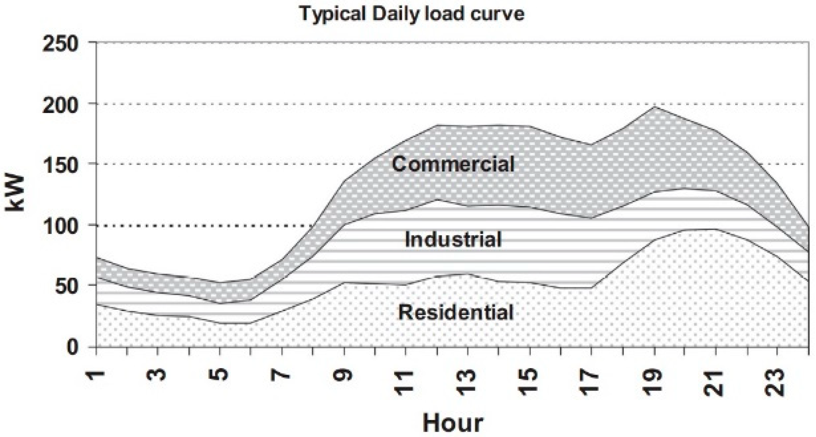
5.1. Data and Assumptions

We have conducted experiments on the system under study based on datasets derived from existing sources [15,16,17,40]. The employed data are visualized in Figure 5, Figure 6, Figure 7 and Figure 8 and presented in

Table 1. Input data for the DGs and the EHs within the case study.

Units	Min. Capacity [kW]	Max. Capacity [kW]	ai [EUR ct/h]	bi [EUR ct/kWh]	ci [EUR ct/kWh2]
MT	6	30	0.01	4.37	0.01
FC	3	30	0.8415	2.41	0.033
WT	0	15	0	0	0
PV1	0	3	0	0	0
PV2…PV5	0	2.5	0	0	0
CHP	10	286	10	3.738	0
Boiler	0	80	0.001	5.098	0

. In detail, Table 1 provides the minimum and maximum capacities in kW for each system unit. Further assumptions that are made for deriving an optimal solution to the Optimal Load Distribution are linked to the power production bids, calorific value of gas, and load demand variations. These assumptions are listed as follows:

➢

Each microsource submits a bid for producing electric power, noted as cost_DG(x_i), where x_i represents the power output for the i = 1…N_DG units as the MT, FC, and boilers. The formula for operation/production costs is expressed as cost_DG(x_i) = a_i + b_i·x_i + c_i·x²_i. The term a_i symbolizes the fixed portion of fuel consumption, including start-up costs if the i-microsource is not utilized during the bidding process, and it is measured in EUR ct/h. The coefficients bi and ci are the variable production costs, expressed in EUR ct/kWh and EUR ct/kWh², respectively.

➢

The output power of the CHP units is dictated by the natural gas input.

➢

The power factor is established at 1 for the PVs and WT, 0.90 for the MT, maintained at 1 for the FC, and set at 0.9 for the CHP units. Additionally, the power factor for the load is assumed to be 0.88.

➢

The calorific value of the input gas, indicated as CV = 0.01115 MWh/Nm³, measures the amount of energy produced from combusting a given volume of gas. In this case, it is calculated based on megawatt-hours (MWh) per normal cubic meter (Nm³) of gas while its cost is assumed to be 0.62 EUR/m³. Hence, the price for each MWh of gas is Cost_{MWh_gas_input} = 55.61 EUR/MWh.

➢

The thermal loads are depicted by hourly figures derived from the established district heating network in northern Greece, according to data sourced from [40].

The optimization problem of OPF with EHs, which focuses on minimizing operational costs, includes the objective function and specific constraints outlined in Section 4. For resolving this optimization problem in the Matlab environment, the Lagrange Multiplier, PSO, and HS methods are employed. The model has been validated in terms of the results it produces in small-scale and simpler scenarios of LV networks as smart homes, where a result/solution reference is present. As an outcome, it exhibits similar results to the actual system.

The validity of the produced results has yet to be verified in a real SM system and due to the complexity of installing and configuring all the energy carriers of such a system, we opted for initially testing our model in the Matlab/Simulink environment using the software version R2023b. However, to enhance the accuracy of the developed optimization model, in this case study, we used real operational data from existing sources [15,16,17,40], aiming to produce realistic results that are also applicable to existing SM systems. Furthermore, deploying such an SM system and comparing the results is part of our ongoing work.

Moreover, for including EV charging in the case study, we gathered real charging data from a Volkswagen ID3 EV as well as a Siemens Versicharge three-phase AC charger [41] that was deployed in the laboratory premises of the Public Power Corporation. These data measured the kW that was used to charge the EV starting from 11 kW and reducing gradually when the battery charge percentage increased substantially. The percentage was measured through the EV battery’s State of Charge (SoC), which is illustrated in Figure 9. Furthermore, we have used these data as the input in the optimization model.

• Scenarios and employed algorithms

We have performed experiments for five unique operational scenarios described accordingly:

○

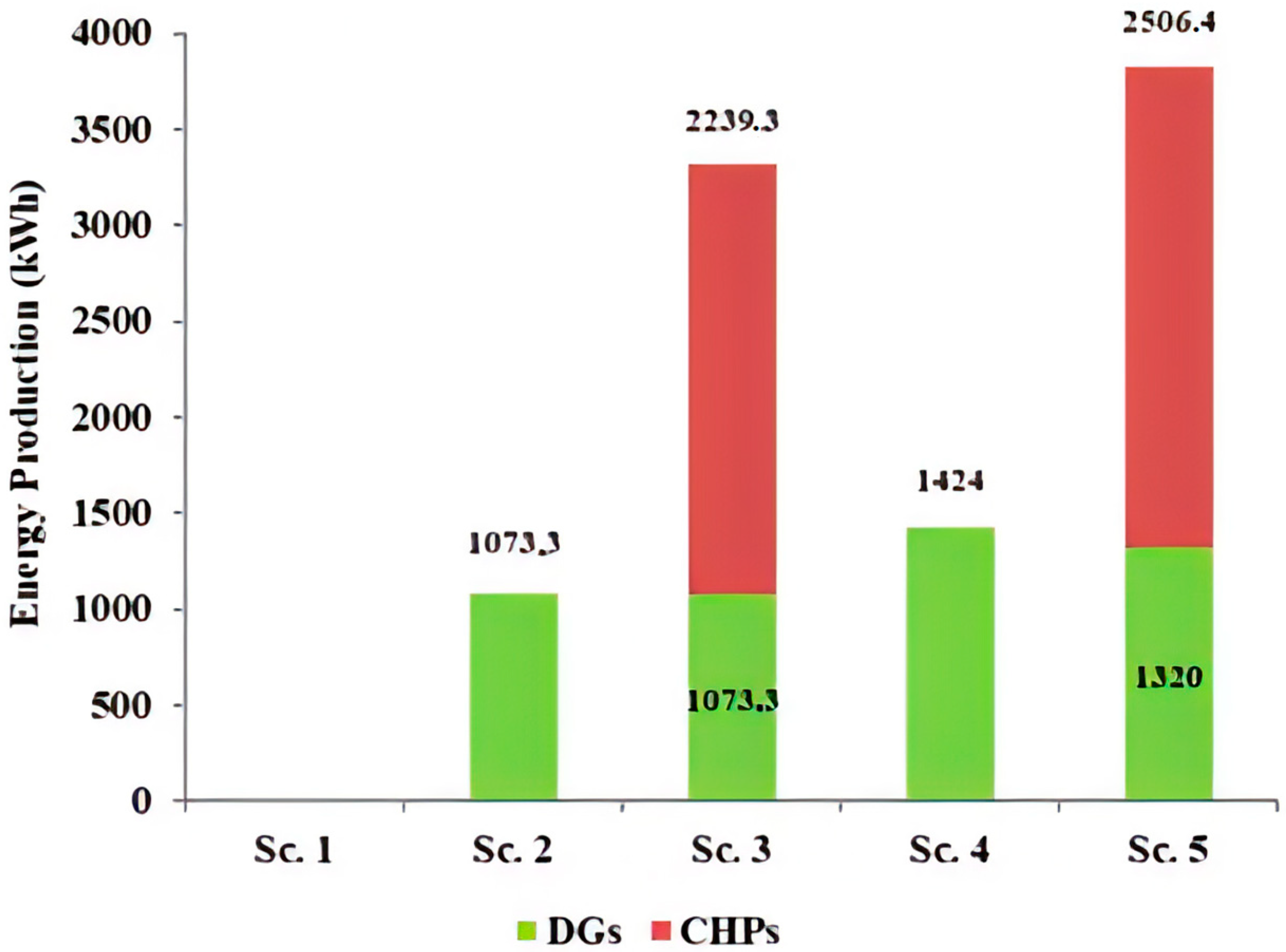
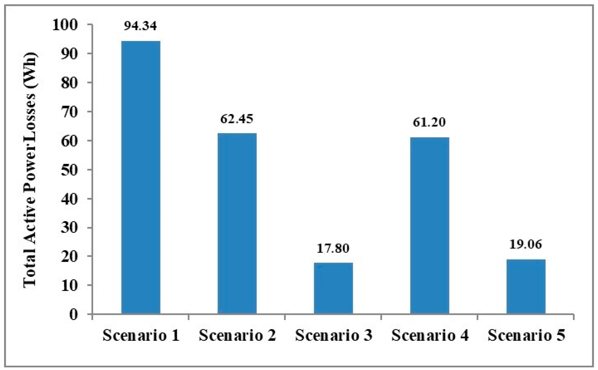
Scenario 1—No DG units and no CHP systems (No-DG).

○

Scenario 2—DG units operating independently (I-DG) without any CHP systems.

○

Scenario 3—DG units operating independently (I-DG) but with CHP systems.

○

Scenario 4—SM operation without CHP systems.

○

Scenario 5—SM operation including CHP systems (SG-EH) along with Electric Vehicles (EVs) and charging stations.

For each scenario, we have executed the three algorithms introduced in Section 4, namely the Lagrange Multiplier, PSO, and HS, to derive the OPF calculation in the system under study. Initially, the Lagrange Multiplier uses as input the generation cost and constraints as the power balance at each EH node to form a linear combination for the gradients of the constraints, in order to ultimately identify a local optimum subject to these constraints. This is performed by introducing auxiliary variables (i.e., the Lagrange Multipliers) for each constraint, in order to minimize the total power production cost while satisfying the demand at each LV distribution network node.

Then, for the PSO algorithm, the particle solutions are identified, and then by exploring the particle search space, to adjust their positions according to the data and assumptions of Section 5.1, a solution is identified, which, as mentioned in Section 4.1, is not the global optimum; nevertheless, it is appropriate for handling the multiple parameters/constraints of our approach. To accomplish this, each particle is initialized with a random position within the feasible solution space and a random velocity, determining how the particle moves into the solution space. The position must adhere to all OPF constraints, such as the capacities of production units and load balance requirements. Moreover, the PSO algorithm adheres to certain parameters such as the Inertia Weight (ω), controlling how the previous velocity influences the current; the Cognitive Coefficient (c1), determining how the best position influences the current; and, lastly, the Social Coefficient (c2), specifying how the global best position influences the velocity update. Furthermore, the operational process of the algorithm allows for an update of a particle position. Specifically, whenever the new position of a particle provides a better solution than its personal best position, then its personal best is updated into this new position. Likewise, if any particle achieves a better solution than the current global best, the global best is updated according to this position. Overall, the main objective of this algorithm and the identified solution is to minimize costs or maximize efficiency in load distribution.

Finally, the HS identifies the optimal solution by continuously selecting harmonies that satisfy the constraints, in order to reach a solution. Then, whenever a better harmony is reached (i.e., it offers a lower cost in terms of power distribution), the worst harmony is replaced. The identified solutions are also linked with algorithm components, as initially, the Harmony Memory Considering Rate (HMCR) specifies the likelihood of considering existing solutions and selecting a new one based on the existing ones; or, if HMCR is not used, the solutions are selected randomly. The second algorithm component is the Pitch Adjusting Rate (PAR), which determines the frequency of adjustments towards exploring the solution neighborhood for potential improvements. The third component is the bandwidth, which determines the degree of adjustments in the harmony, thus allowing enhanced exploration capabilities. To further improve the Harmony Search algorithm, we also employed the technique mentioned in [42], in order to allow for the solving of Economic Dispatch problems.

Overall, each of the three algorithms is capable of identifying different solutions for OPF calculation. Specifically, the Lagrange Multiplier allows one to identify the local optimum solution and the PSO uses it as a particle and is executed toward specifying the global optimum. Afterward, the HS obtains the solutions of the Lagrange Multiplier and the PSO as the existing solutions (i.e., harmonies) and through an iterative process, identifies the global optima. This is followed for each aforementioned scenario and is performed during the experiments of the following section.

5.2. Experiments

Figure 10 and Figure 11 illustrate the superiority of scenarios 3 and 5, respectively. The integration of Energy Distributors into the SM highlights the significant role of CHP units, which contribute to the independence from the main grid. Such integration enhances the “islanding” capability of the SM in the event of an upstream system fault. Notably, when natural gas prices drop below those of electricity in the main grid, there is a noticeable reduction in energy expenses.

Figure 12 presents the total active losses of the system, while Figure 13 depicts the coverage of the thermal load. It is evident that the thermal load is almost entirely covered by the CHP units in scenarios 3 and 5, and not by the boilers.

The results indicate that the combined consideration of SΜs and EHs offers the most advantages for consumers, the environment, and the overall energy system. This achieves a reduction in energy costs of 21.2% compared to the worst-case scenario, a decrease in power losses of 79.8%, and a reduction in incoming power from the swing bus of 87.5%. These significant reductions in power losses and incoming power from the interconnected system have positive impacts on the environment due to the reduction in harmful gas emissions.

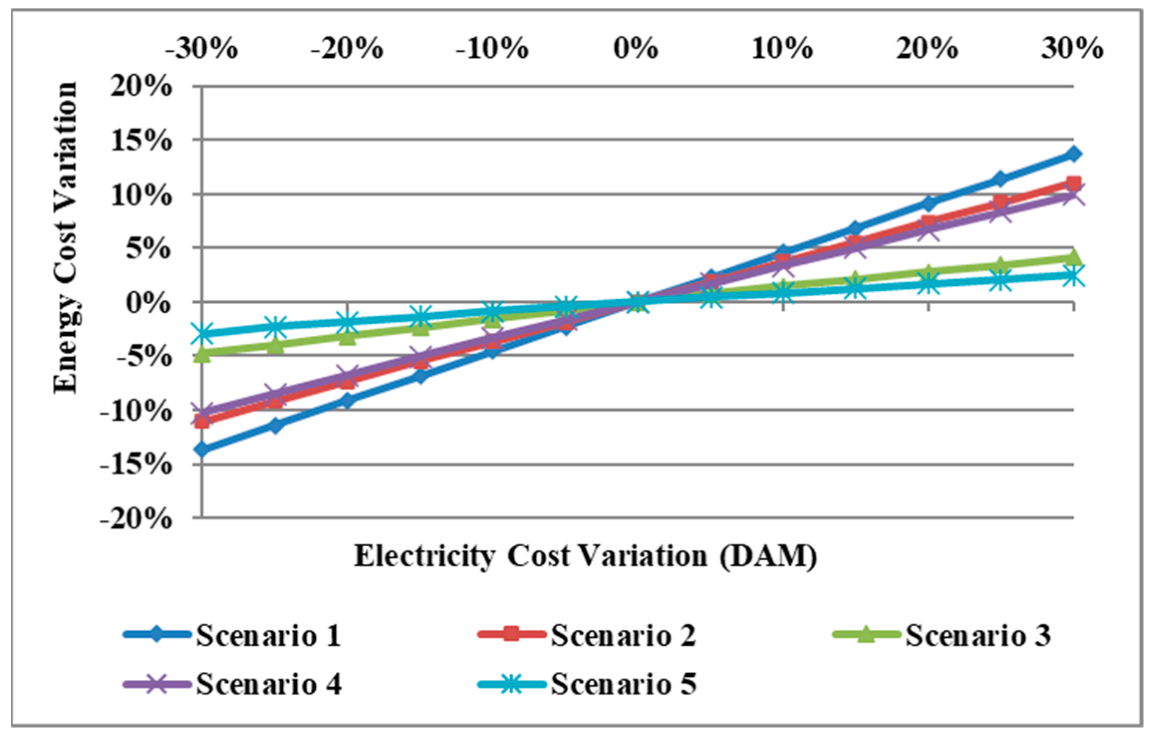
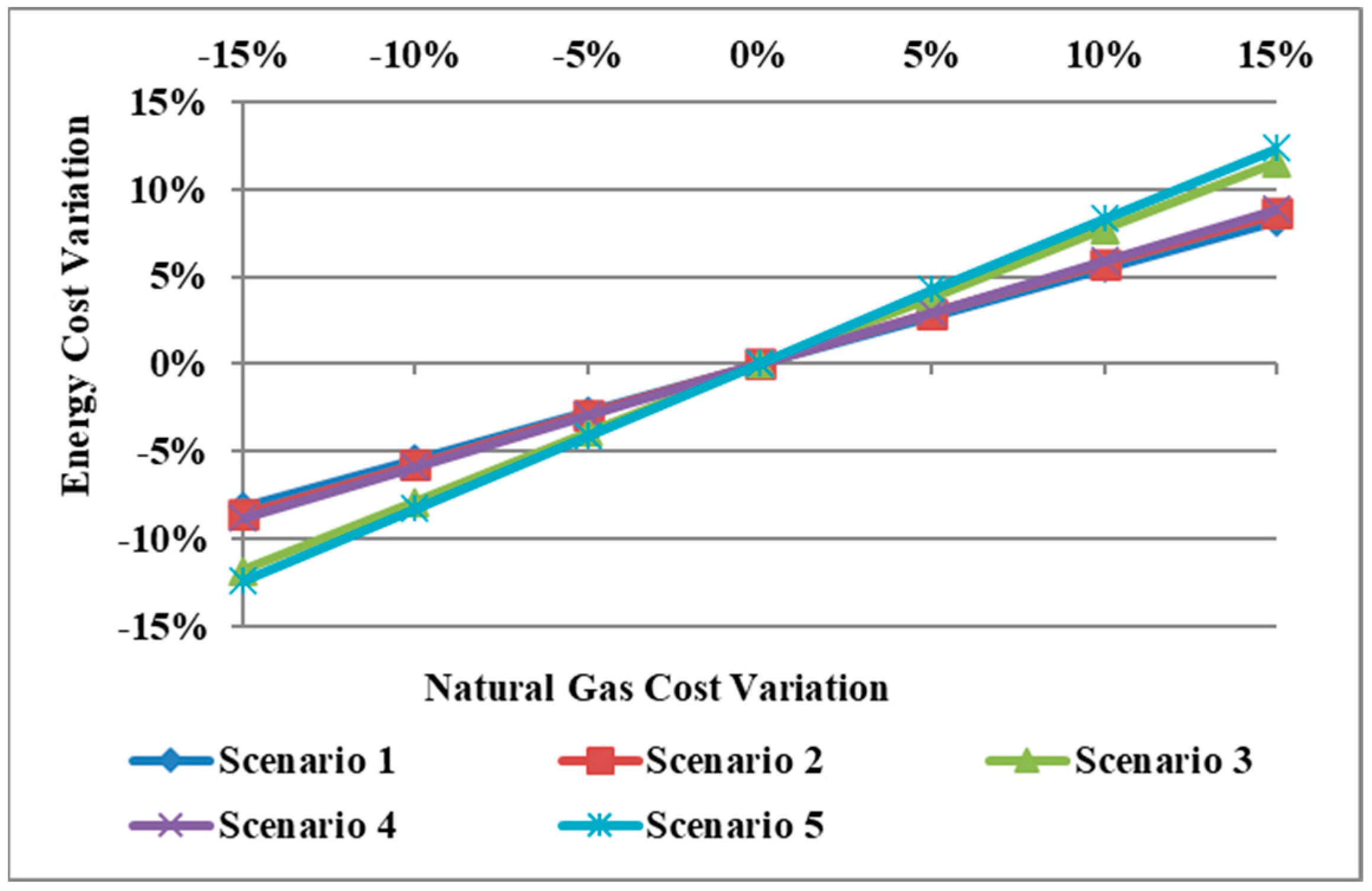
5.3. Sensitivity Analysis

Sensitivity analysis examines the impact of modifying key parameters of the optimization model (such as energy prices or demand levels), and through the results, the objective is to understand robustness and identify critical factors influencing system behavior. In this section, we have experimented with the cost variation for different energy sources, such as electricity, and natural gas along with electrical and thermal demand. In the following part, the results for each of the operational scenarios are presented.

• Electricity Cost Variation

The electricity cost variation is depicted in Figure 14, where scenario 5 exhibits the lowest sensitivity (EUR/MWh), in contrast to the other scenarios, due to its lower dependency. Specifically, scenario 5 provides the best conditions for the operation of the system under any variation in electricity costs, achieving a reduction of up to 28.9% compared to scenario 1.

• Natural Gas Cost Variation

The natural gas cost variation is depicted in Figure 15, where it is observed that scenario 5 remains the most economical for the system under study. However, the underlying difference here is that the greatest change in the total energy cost is seen in scenario 5, followed by scenario 3. This is due to the high dependency on CHP units, which require larger quantities of natural gas. Scenarios 1, 2, and 4 are less affected by changes in the cost of natural gas because they only involve boilers. Thus, the amount of natural gas imported is smaller in these scenarios compared to the others.

• Electrical and Thermal Load Demand Variation

The load demand usually increases annually, and there may also be seasonal variations. This case study addresses the electrical and thermal demand loads of the examined network, which are also simultaneously changed. Such changes range between −50% and +50%, hence having a significant impact on the total system energy cost, as shown in Figure 16. Additionally, from this figure, it is observed that when the demand load decreases, all scenarios reach a satisfactory convergence. The main problem arises when the load increases, where similarly with the electricity and natural gas variation, scenario 5 performs the best in handling increased demand.

6. Summary and Conclusions

This article proposes a new approach for modeling the behavior of EHs that integrate MECs in an LV SM network. The model is used to derive an optimization problem, formed through a combination of (1) the OPF for an SM and (2) the Optimal Load Distribution for energy distributors considering various energy sources, such as CHP units, RES, and energy storage systems. The method is applied in a typical Greek 17-bus LV distribution network, where the Lagrange Multiplier, PSO, and HS algorithms were used to derive the solution in the Matlab environment. Multiple operational scenarios are examined and through a sensitivity analysis, Optimal Load Distribution is achieved in the presence of RES and EV chargers. Moreover, in all operational scenarios, the OPF solution demonstrated that the security limits of the electrical network were always satisfied.

Additionally, the article also described boundary conditions for converting the energy from one source to another for the proposed method as (1) load demand prediction, (2) the performance of devices used for the conversion as inverters and transformers, (3) the market prices for electricity and gas energy, and (4) the presence of RES and energy storage mechanisms used as an additional energy supply source to cope with peak load demand instead of switching between different energy sources. Similarly, constraints were also defined for the model’s use in calculating the Optimal Load Distribution. The identified constraints relate initially to the ML model accuracy for the prediction of load demand, impacted by the amount of gathered historical electrical and thermal energy consumption data as well as indoor and outdoor temperature, indoor and outdoor humidity, and global horizontal radiation data for training the ML models. Additionally, apart from the model accuracy and the selection of the ML model, a very important constraint relates to the integration with energy market platforms, in order to retrieve real-time price data. In the considered case study, we have only derived electrical energy consumption data, and the thermal data were based on hourly figures derived from the established district heating network in northern Greece. This is due to imposed restrictions on the deployed households and as a consequence, it impacts the ML model prediction accuracy. Hence, we consider it a considerable limitation that is planned to be addressed in our future work. Another limitation lies in the validation of the proposed approach, which occurs through the Matlab simulation environment.

To address the limitation of validating the proposed approach, we plan to use the smart home area network testbed that is already present in the Innovation Hub of PPC with a coal-based generator serving a sufficiently large habitat area, RESs, EV chargers, and a battery system for energy storage [40]. This testbed is flexible and can be extended to form an SM by including CHP and further distributed generation units. Furthermore, the testbed will be used to conduct the operational scenarios that were implemented in the Matlab environment in this article, hence allowing the approach in a real SM setup. Moreover, since we consider that the SMs equipped with MECs are expected to offer a broad field of study and research in future electrical and natural gas networks, through this deployment we will be able to conduct the scenarios in a real SM where actual loads from production systems will be incorporated and the proposed method will be used for calculating OPF calculation and the Optimal Load Distribution. Moreover, we plan to address the boundary conditions of the proposed approach, which, apart from the accuracy in the load demand prediction, also lies in the integration with energy market platforms to retrieve real-time energy price data about each energy source within the EH.

References

1. European Commission. The European Green Deal, Brussels. Available online: https://eur-lex.europa.eu/resource.html?uri=cellar:b828d165-1c22-11ea-8c1f-01aa75ed71a1.0002.02/DOC_1&format=PDF (accessed on 16 May 2024).
2. European Commission. Fit for 55: Delivering the EU’s 2030 Climate Target on the Way to Climate Neutrality, Brussels. Available online: https://eur-lex.europa.eu/legal-content/EN/TXT/PDF/?uri=CELEX:52021DC0550&from=EN (accessed on 16 May 2024).
3. Li, C.; Wang, N.; Wang, Z.; Dou, X.; Zhang, Y.; Yang, Z.; Maréchal, F.; Wang, L.; Yang, Y. Energy hub-based optimal planning framework for user-level integrated energy systems: Considering synergistic effects under multiple uncertainties. Appl. Energy 2022, 307, 118099. [Google Scholar] [CrossRef]
4. Geidl, M.; Koeppel, G.; Favre-Perrod, P.; Klöckl, B.; Andersson, G.; Fröhlich, K. Energy Hubs for the Future. IEEE Power Energy Mag. 2007, 5, 24–30. [Google Scholar] [CrossRef]
5. Geidl, M.; Andersson, G. Optimal Power Flow of Multiple Energy Carriers. IEEE Trans. Power Syst. 2007, 22, 145–155. [Google Scholar] [CrossRef]
6. Mohammadi, M.; Noorollahi, Y.; Mohammadi-Ivatloo, B.; Yousefi, H. Energy hub: From a model to a concept—A review. Renew. Sustain. Energy Rev. 2017, 80, 1512–1527. [Google Scholar] [CrossRef]
7. Papadimitriou, C.N.; Anastasiadis, G.A.; Psomopoulos, C.S.; Vokas, G. Demand Response schemes in Energy Hubs: A comparison study. Energy Procedia 2019, 157, 939–944. [Google Scholar] [CrossRef]
8. Hatziargyriou, N.; Asano, H.; Iravani, R.; Marnay, C. Microgrids. IEEE Power Energy Mag. 2007, 5, 78–94. [Google Scholar] [CrossRef]
9. Guerrero, J.M.; Vasquez, J.C.; Savaghebi, M.; Castilla, M. Hierarchical control of droop-controlled AC and DC microgrids—A general approach toward standardization. IEEE Trans. Ind. Electron. 2013, 60, 1254–1262. [Google Scholar] [CrossRef]
10. Wang, S.; Wang, X.; Li, X.; Liu, X. Optimal energy management of microgrids with renewable energy and energy storage under uncertainty. Energy 2016, 96, 160–169. [Google Scholar]
11. Lasseter, R.H.; Akhil, A.A.; Marnay, C.; Stephens, J.; Dagle, J.E.; Guttromson, R.; Meliopoulous, A.; Yinger, R.; Eto, J.; Piagi, P. Integration of distributed energy resources: The CERTS microgrid concept. Electr. J. 2007, 20, 26–38. [Google Scholar]
12. Mohammadi, M.; Noorollahi, Y.; Mohammadi-Ivatloo, B. An Introduction to Smart Energy Systems and Definition of Smart Energy Hubs. In Operation, Planning, and Analysis of Energy Storage Systems in Smart Energy Hubs; Springer: Cham, Switzerland, 2018. [Google Scholar]
13. Sari, A.; Lekidis, A.; Butun, I. Industrial Networks and IIoT: Now and Future Trends. Industrial IoT: Challenges, Design Principles, Applications, and Security; Springer Nature: Cham, Switzerland, 2020; pp. 3–55. [Google Scholar]
14. Olivares, D.E.; Mehrizi-Sani, A.; Lopes, L.A. Smart microgrids: A review of technologies, applications and operational challenges. Renew. Sustain. Energy Rev. 2014, 51, 975–993. [Google Scholar]
15. Anastasiadis, A.G.; Vokas, G.A. Economic benefits of Smart Microgrids with penetration of DER and mCHP units for non-interconnected islands. Renew. Energy 2019, 142, 478–486. [Google Scholar] [CrossRef]
16. Hatziargyriou, N.D.; Anastasiadis, G.A.; Vasiljevska, J.; Tsikalakis, A.G. Quantification of Economic, Environmental and Operational Benefits of Microgrids. In Proceedings of the IEEE PowerTech, Bucharest, Romania, 28 June–2 July 2009; p. 512. [Google Scholar] [CrossRef]
17. Anastasiadis, A.G.; Konstantinopoulos, S.; Kondylis, G.P.; Vokas, G.A. Electric vehicle charging in stochastic smart microgrid operation with fuel cell and RES units. Int. J. Hydrogen Energy 2017, 42, 8242–8254. [Google Scholar] [CrossRef]
18. Mohammadi, M.; Noorollahi, Y.; Mohammadi-ivatloo, B.; Hosseinzadeh, M.; Yousefi, H.; Khorasani, S.T. Optimal management of energy hubs and smart energy hubs—A review. Renew. Sustain. Energy Rev. 2018, 89, 33–50. [Google Scholar] [CrossRef]
19. Maroufmashat, A.; Taqvi, S.T.; Miragha, A.; Fowler, M.; Elkamel, A. Modeling and optimization of energy hubs: A comprehensive review. Inventions 2019, 4, 50. [Google Scholar] [CrossRef]
20. Javadi, M.S.; Lotfi, M.; Nezhad, A.E.; Anvari-Moghaddam, A.; Guerrero, J.M.; Catalão, J.P. Optimal operation of energy hubs considering uncertainties and different time resolutions. IEEE Trans. Ind. Appl. 2020, 56, 5543–5552. [Google Scholar] [CrossRef]
21. Kienzle, F.; Ahčin, P.; Andersson, G. Valuing investments in multi-energy conversion, storage, and demand-side management systems under uncertainty. IEEE Trans. Sustain. Energy 2011, 2, 194–202. [Google Scholar] [CrossRef]
22. Unsihuay-Vila, C.; Marangon-Lima, J.W.; de Souza, A.C.Z.; Perez-Arriaga, I.J.; Balestrassi, P.P. A model to long-term, multiarea, multistage, and integrated expansion planning of electricity and natural gas systems. IEEE Trans. Power Syst. 2010, 25, 1154–1168. [Google Scholar] [CrossRef]
23. Ji-Yuan, F.; Lan, Z. Real-time economic dispatch with line flow and emission constraints using quadratic programming. IEEE Trans. Power Syst. 1998, 13, 320–325. [Google Scholar] [CrossRef]
24. Farag, A.; Al-Baiyat, S.; Cheng, T.C. Economic load dispatch multiobjective optimization procedures using linear programming techniques. IEEE Trans. Power Syst. 1995, 10, 731–738. [Google Scholar] [CrossRef]
25. Dhillon, J.S.; Parti, S.C.; Kothari, D.P. Stochastic economic emission load dispatch. Electric Power Syst. Res. 1993, 26, 186–197. [Google Scholar] [CrossRef]
26. Yokoyama, R.; Bae, S.H.; Morita, T.; Sasaki, H. Multiobjective generation dispatch based on probability security criteria. IEEE Trans. Power Syst. 1988, 3, 317–324. [Google Scholar] [CrossRef]
27. Zia, M.F.; Elbouchikhi, E.; Benbouzid, M. Microgrids energy management systems: A critical review on methods, solutions, and prospects. Appl. Energy 2018, 222, 1033–1055. [Google Scholar] [CrossRef]
28. Sadeghi, A.R.; Wachsmann, C.; Waidner, M. Security and privacy challenges in industrial internet of things. In Proceedings of the 52nd Annual Design Automation Conference, San Francisco, CA, USA, 7–11 June 2015; pp. 1–6. [Google Scholar]
29. Momoh, J.A.; Koessler, R.J.; Bond, M.S.; Stott, B.; Sun, D.; Papalexopoulos, A.; Ristanovic, P. Challenges to Optimal Power Flow. IEEE Trans. Power Syst. 1997, 12, 444–447. [Google Scholar] [CrossRef]
30. Huneault, M.; Galiana, F.D. A Survey of the Optimal Power Flow Literature. IEEE Trans. Power Syst. 1991, 6, 762–770. [Google Scholar] [CrossRef]
31. Kuhn, H.W.; Tucker, A.W. Nonlinear programming. In Proceedings of the 2nd Berkeley Symposium on Mathematical Statistics and Probability, Berkeley, CA, USA, 31 July–12 August 1951. [Google Scholar]
32. Horst, Ρ.; Pardalos, P.M. Handbook of Global Optimization (Nonconvex Optimization and Its Applications, 2), 1995th ed.; Kluwer Academic Publishers: Dordrecht, The Netherlands, 2002. [Google Scholar]
33. Pardalos, P.M.; Resende, M.G.C. Handbook of Applied Optimization; Oxford University Press: Oxford, UK, 2002; ISBN 0-19-512594-0. [Google Scholar]
34. Lekidis, A.; Papageorgiou, E.I. Edge-based short-term energy demand prediction. Energies 2023, 16, 5435. [Google Scholar] [CrossRef]
35. Carpentier, J. Optimal power flows. Int. J. Electr. Power Energy Syst. 1979, 1, 3–15. [Google Scholar] [CrossRef]
36. Wood Allen, J.; Wollenberg Bruce, F. Power Generation, Operation and Control, 2nd ed.; John Wiley & Sons: New York, NY, USA, 1996; p. 104. [Google Scholar]
37. Costa, V.M.; Martins, N.; Pereira, J.L.R. Developments in the Newton Raphson Power Flow Formulation Based on Current Injections. IEEE Trans. Power Syst. 1999, 14, 1320–1326. [Google Scholar] [CrossRef]
38. Katiraei, F.; Iravani, M.R.; Lehn, P.W. Micro-grid autonomous operation during and subsequent to islanding process. IEEE Trans. Power Deliv. 2005, 20, 248–257. [Google Scholar] [CrossRef]
39. Schaffer, M.; Veit, M.; Marszal-Pomianowska, A.; Frandsen, M.; Pomianowski, M.Z.; Dichmann, E.; Sørensen, C.G.; Kragh, J. Dataset of smart heat and water meter data with accompanying building characteristics. Data Brief 2024, 52, 109964. [Google Scholar] [CrossRef]
40. Hellenic Public Power Corporation, S.A. Available online: www.dei.gr (accessed on 16 May 2024).
41. Lekidis, A.; Papageorgiou, I.E. Risk Assessment Method for 5G-oriented DLMS/COSEM Communications. In Proceedings of the ΙΕΕΕ Conference on Standards for Communications and Networking (CSCN), Munich, Germany, 6–8 November 2023. [Google Scholar]
42. dos Santos Coelho, L.; Mariani, V.C. An improved harmony search algorithm for power economic load dispatch. Energy Convers. Manag. 2009, 50, 2522–2526. [Google Scholar] [CrossRef]
Figure 1. EH architecture with input and output sources as well as transformation and management equipment (based on [5]).
Energies 17 02827 g001
Figure 2. Energy Management System architecture for Energy Hub management.
Energies 17 02827 g002
Figure 3. The case-study LV distribution network overview (based on [15]).
Energies 17 02827 g003
Figure 4. Overview of the two EHs employed in this case study.
Energies 17 02827 g004
Figure 5. Power output from the WT and PVs with comparable graphs for every day of the year.
Energies 17 02827 g005
Figure 6. Standard load profile for each feeder in the case study network.
Energies 17 02827 g006
Figure 7. Yearly trends of the System Marginal Price (now, Day-Ahead Market—DAM).
Energies 17 02827 g007
Figure 8. Electrical (nge) and thermal efficiency (ngh) data of the CHP units.
Energies 17 02827 g008
Figure 9. State of Charge on the EV battery used as data input for the case study.
Energies 17 02827 g009
Figure 10. Energy cost per hour for a typical day.
Energies 17 02827 g010
Figure 11. Energy production of DGs and CHPs for a typical day.
Energies 17 02827 g011
Figure 12. Total active power losses for a typical day.
Energies 17 02827 g012
Figure 13. Thermal power production from CHPs for a typical day.
Energies 17 02827 g013
Figure 14. Electricity cost variation (DAM) for a typical day.
Energies 17 02827 g014
Figure 15. Natural gas cost variation for a typical day.
Energies 17 02827 g015
Figure 16. Total energy cost variation of various scenarios compared to scenario 1 for a typical day.
Energies 17 02827 g016