Article

Optimizing Mixed-Model Synchronous Assembly Lines with Bipartite Sequence-Dependent Setup Times in Advanced Manufacturing

by
Asieh Varyani
1,
Mohsen Salehi
2 and
Meysam Heydari Gharahcheshmeh
3,*
1
Department of Mechanical, Industrial, and Manufacturing Engineering, Oregon State University, SW Monroe Avenue, Corvallis, OR 97331, USA
2
Department of Industrial Engineering, Faculty of Engineering, Bu-Ali Sina University, Hamedan 6517838623, Iran
3
Department of Mechanical Engineering, San Diego State University, 5500 Campanile Drive, San Diego, CA 92182, USA
*
Author to whom correspondence should be addressed.
Energies 2024, 17(12), 2865; https://doi.org/10.3390/en17122865
Submission received: 6 May 2024 / Revised: 1 June 2024 / Accepted: 5 June 2024 / Published: 11 June 2024
(This article belongs to the Section K: State-of-the-Art Energy Related Technologies)

Abstract

:
In advanced manufacturing, optimizing mixed-model synchronous assembly lines (MMALs) is crucial for enhancing productivity and adhering to sustainability principles, particularly in terms of energy consumption and energy-efficient sequencing. This paper introduces a novel approach by categorizing sequence-dependent setup times into bipartite categories: workpiece-independent and workpiece-dependent. This strategic division streamlines assembly processes, reduces idle times, and decreases energy consumption through more efficient machine usage. A new mathematical model is proposed to minimize the intervals at which workpieces are launched on an MMAL, aiming to reduce operational downtime that typically leads to excessive energy use. Given the Non-deterministic Polynomial-time hard (NP-hard) nature of this problem, a genetic algorithm (GA) is developed to efficiently find solutions, with performance compared against the traditional branch and bound technique (B&B). This method enhances the responsiveness of MMALs to variable production demands and contributes to energy conservation by optimizing the sequence of operations to align with energy-saving objectives. Computational experiments conducted on small and large-sized problems demonstrate that the proposed GA outperforms the conventional B&B method regarding solution quality, diversity level, and computational time, leading to energy reductions and enhanced cost-effectiveness in manufacturing settings.

1. Introduction

The necessity of addressing climate change, which targets a reduction in carbon dioxide (CO2) emissions, alongside stricter regulations, has prompted extensive research into energy efficiency and renewable energy sources [1,2,3,4]. Ensuring that all economic sectors achieve zero CO2 emissions by the second half of this century (with a target of 2060) is essential for limiting the increase in the global average temperature to 1.5 °C [5]. Manufacturing industries heavily depend on energy resources to supply fuel and power to transform raw materials into final products or services, contributing significantly to greenhouse gas emissions. The efficiency, cost, and accessibility of energy emerge as critical factors influencing manufacturers’ competitiveness and economic resilience [2,6]. Enhanced energy efficiency within manufacturing reduces costs, preserves finite energy reserves, and enhances productivity. Furthermore, improved energy efficiency provides additional environmental benefits, particularly in mitigating emissions of greenhouse gases and air pollutants.
In the United States, the industrial sectors, which account for 33% of all energy consumption [7], are struggling with challenges stemming from global supply chain issues, such as semiconductor shortages [8]. In response, manufacturers are directing their focus toward researching and developing long-term strategies to enhance the energy efficiency of production notably. Improving competitiveness and sustainability in all industry sectors, including semiconductor manufacturing, is crucial for securing market share and ensuring business success. This is particularly evident in semiconductor manufacturing, which utilizes various chemical vapor deposition (CVD) methods [9,10,11] for both inorganic semiconductors [9,12] and organic conducting polymers [11,13,14,15,16,17,18] across a wide range of electronic and optoelectronic applications.
In CVD-based manufacturing, multiple process parameters must be controlled and monitored to ensure the quality of the final products, particularly when stacking different layers to form the final device [9,10,19]. Enhanced manufacturing processes can reduce rework, cycle time, and energy consumption. However, achieving effective process control in the semiconductor industry is challenging due to the complex processes and high precision required. Additionally, semiconductor manufacturing typically has long production cycle times. Efforts to reduce the overall cycle time of fabrication lines are closely linked to improving overall productivity and enhancing the competitiveness and sustainability of semiconductor manufacturing. Improving performance measurement in these complex fabrication lines necessitates sound judgment and decision-making regarding lot release policies and scheduling of work on machines.
The move toward large-scale customization in energy device manufacturing, driven by consumer demand, marks a departure from the ‘one-size-fits-all’ approach of the 1980s, which focused on standardized components and work optimization to produce uniform products economically [20]. While this model initially expanded market access, it could not meet the rising demand for personalized products due to their inflexibility, which prompted a shift towards customization [21]. This trend is especially pronounced in certain industries, characterized by a significant expansion in product accessory variety [22,23].
Energy device manufacturing industries increasingly adopt mixed-model assembly lines (MMALs) to accommodate such diversity. The MMAL is a particular case of manufacturing lines where different models of the same products are mixed and then assembled on the same line [24]. This adaptation necessitates focusing on mixed or multi-model assembly lines within manufacturing industries, as these systems offer the flexibility required to assemble a wide range of product variants [20]. MMALs can operate differently, including paced or unpaced lines [25]. In paced lines, the cycle time (throughput rate) is set externally, limiting operators’ time to work on each job [26]. If this allocated time elapses before the task is complete, the workpiece must move on, potentially leaving some tasks unfinished at their designated stations [27]. In contrast, Unpaced lines place no such time limits on task completion, allowing for more flexibility [26].
Research on MMAL sequencing has primarily focused on paced assembly lines, for example, [28,29,30,31,32,33,34,35,36,37,38,39,40,41,42,43,44,45,46,47,48]. This study is focused on unpaced assembly line configurations, which can be categorized as synchronous or asynchronous [25]. In unpaced asynchronous lines, buffer stocks serve to decouple stations, storing workpieces while the next station is occupied with earlier tasks [27]. This arrangement means that the movement of workpieces between adjacent stations is not synchronized. Each workpiece will begin its process at a station whenever that station is free, and once its processing is completed, it moves on from the station [49]. In unpaced synchronous lines, the transfer of workpieces between stations is carefully coordinated, ensuring that all workpieces move simultaneously [27]. This coordinated transfer waits for a signal confirming the completion of tasks at all stations before moving [50]. Unpaced synchronous lines are commonly utilized in the automobile industry and are preferred for assembling large products [49]. Despite their widespread use, limited research has focused on unpaced synchronous lines. Therefore, this study is concentrated on unpaced synchronous assembly lines.
Kouvelis and Karabati [49] introduced the sequencing problem synchronously by running unpaced lines, adopting a cyclic scheduling approach to minimize the line’s cycle time. They developed an integer programming model for the problem and introduced an approximate solution method. Additionally, they indicated the Non-deterministic Polynomial-time hard (NP-hard) nature of the problem. Karabati and Tan [51] explored the sequencing problem in synchronous assembly lines, assuming processing times are random independent variables. Their focus was on minimizing cycle time (maximizing throughput rate) as the primary objective. They outlined a scheduling procedure and introduced two heuristics for a broader spectrum of the problem. Salehi et al. [50] studied the sequencing of unpaced synchronous assembly lines to minimize three objectives: total setup cost, total production rate variation cost, and total idle cost. They assigned importance weights to each objective and developed a mathematical model to address the problem.
In the manufacturing industry, the capacity to rapidly adapt production lines to accommodate a different range of products is crucial for maintaining competitive advantage [52]. Two critical aspects in optimizing MMALs are line design and the balancing and sequencing of product models [53]. The mixed-model line design and balancing involve assigning tasks for all models to the workstations, considering the given precedence relationships among the tasks [54]. The sequencing problem entails determining the order in which different product models are launched down the assembly line.
Mixed-model scheduling often emerges as a challenge in just-in-time (JIT) manufacturing for energy devices. It involves determining the optimal production sequence for multiple products on the same assembly line, essential for keeping inventory levels low [54]. The success of JIT systems depends on ensuring that the correct parts are in the right place at the right time, achieved by creating a schedule that promotes a steady flow of materials and parts across the assembly line [54]. This process involves minimizing setup times, including tasks like changing tools and setting up machines [52]. While these activities may not add direct value to the product, they enable manufacturers of energy devices to meet market demands efficiently [45].
However, it is often assumed that the setup times required for changing the assembly line from one product model to another are minimal and do not impact overall operations [55]. This assumption is challenged by recent discussions highlighting the critical impact of setup times on scheduling quality, especially when assembly stations operate near total capacity [56]. The significance of scheduling models that account for setup times has been explored in multiple studies [57,58,59,60]. Separating setup times from processing times enables simultaneous operations, thereby enhancing resource utilization [56]. This approach is in line with the principles of modern production management systems, including JIT, Optimized Production Technology (OPT), and Group Technology (GT), supporting the need for explicit consideration of setup times in scheduling models [61]. Assembly line balancing and sequencing problems are closely connected. However, these two issues are typically addressed separately, likely due to the computational complexities involved [62].
Therefore, assuming the line is already balanced (i.e., all assembly tasks are assigned to stations in accordance with the specified precedence relationships among the tasks), this paper focuses on product model sequencing to support JIT objectives by reducing setup times and ensuring a smooth production process for energy devices.
Setup time refers to the time needed to prepare machines and processes for upcoming workpieces, including tool acquisition, workpiece positioning, and material inspection. In MMAL sequencing, setup time is differentiated into sequence-independent, where time is consistent per product, and sequence-dependent, which varies based on the previous product. Setup times are often added to the processing time in sequence-independent setups [63]. By reviewing previous research, it is evident that most prior work on sequencing MMALs has focused on minimizing the number of setups or sequence-dependent setup costs, with less attention given to sequence-dependent setup times. For instance, Giard and Jeunet [46], Mansouri [64], McMullen and Frazier [65], and McMullan [66,67,68] investigated sequencing MMAL with the objective of minimizing the number of setups. Additionally, Rahimi-Vahed et al. [43], Rahimi-Vahed and Mirzaei [44], Tavakkoli-Moghaddam and Rahimi-Vahed [45], Salehi et al. [50], and Akgündüz and Tunalı [69] addressed the problem of sequencing in MMALs by considering sequence-dependent setup costs.
This paper addresses the sequencing problem in unpaced mixed-model synchronous assembly lines (MMSALs), specifically considering sequence-dependent setup times. Moreover, it introduces a novel consideration by dividing the setup into workpiece-independent and workpiece-dependent categories. The workpiece-independent setup activities can be initiated before the arrival of the workpiece at the station, allowing operators to utilize their time effectively and prepare in advance. In contrast, a workpiece-dependent setup requires the actual workpiece to be present for implementation. No prior studies have divided setup times into these distinct categories, which could offer important insights for optimizing workflow and reducing overall production time in MMALs for energy devices.
This work is among the first in a customized product manufacturing line for energy devices to split sequence-dependent setup times into workpiece-independent and workpiece-dependent categories. This innovative division allows for separating setup activities based on the necessity of having the workpiece present at the station. Additionally, the study develops a new mathematical model to optimize MMALs with bipartite sequence-dependent setup times, focusing on minimizing the intervals between workpiece launches. This is critical for enhancing MMAL efficiency, especially when the configuration of stations is fixed.
The sequencing problem’s combinatorial nature creates a massive number of possible ways to arrange the production sequences, making it very difficult and often impractical to identify the optimal solution [62]. Different methods have been proposed, such as goal-chasing methods [70], dynamic programming [41], tabu search [64], variable neighborhood search [63], linear and integer programming [65], branch and bound [48], ant colony optimization [66], simulated annealing [48,58], genetic algorithms [67,68,69,71,72,73,74], and some other search heuristics [44,75,76]. Among these, genetic algorithms (GAs) have been indicated to be particularly effective in addressing various manufacturing optimization problems [62]. GAs, inspired by biological evolution and the principle of “survival of the fittest”, are particularly adept at solving NP-hard combinatorial optimization problems [62]. The sequencing problems in MMALs are classified as an NP-hard optimization problem, making large-sized instances computationally intractable [77]. Therefore, this study introduces a GA designed to address MMAL large-scale sequencing challenges within acceptable computational times. By incorporating a swapping mutation mechanism, the GA prevents premature convergence and sustains a diverse gene pool, enabling better solution space exploration. Comparative analysis with the B&B technique across small and large problem datasets underscores the GA’s superior performance, highlighting its potential for improving industrial scheduling and sequencing operations.

2. Simulation

2.1. Problem Description and Notations

An MMSAL typically consists of some stations connected by a conveyor belt or similar mechanical handling equipment. In such lines, all workpieces are moved simultaneously from one station to the next after all stations have finished their assigned tasks. Each station holds only one workpiece at any given moment. Once all operators complete their tasks, the conveyor belt advances the workpieces to the next stations and pauses until the next movement. The process awaits a signal confirming the completion of all station tasks before transferring workpieces. Each cycle removes the workpiece in the final station as the finished product, and a new workpiece is introduced at the first station.
Based on the description, the time interval between consecutive movements of the conveyor belt equals the longest task time among the workpieces currently being processed at the stations. Tasks at different stations vary, and their durations may not be equal. Additionally, due to model variations, task times for a given model can differ across stations. Once an operator completes their tasks, they must wait for other station operators to complete their tasks before proceeding. During this waiting period, an operator may start the workpiece-independent portion of the setup for the next workpiece, if possible.
A minimal part set (MPS) production strategy is common in MMALs. MPS defines a product mix through d 1 , , d M = D 1 / h , , D M / h , wherein M represents the total number of models, D M represents the number of products of a model type, m, that need to be assembled over the planning horizon, and h represents the highest common factor or greatest common divisor of D 1 , D 2 , , D M . This strategy operates cyclically. I = i = 1 M d i gives the number of products manufactured for energy devices in one cycle. Specifically, h multiplied by the repetition of manufacturing the MPS products for energy devices meets the total demand in the planning horizon.
Considering K as the number of stations and I as the total number of workpieces (products) in a Minimal Part Set (MPS), the sequence S = P 1 P 2 P I represents a cyclic sequence of workpieces in an MPS, where P l denotes the workpiece in the l-th position of the cycle. Workpieces are introduced to the assembly line in this specified sequence repeatedly, forming a pattern of P 1 P 2 P I P 1 P 2 P I P 1 P 2 P I , with C i ,   i = 1 , ,   I indicating the time interval between the launch of consecutive workpieces, P i 1   P [ i 1 ] d P [ i ] . C 1 is defined as the interval between the current cycle’s last workpiece(product) and the next cycle’s first workpiece. Assuming I > K, Table 1 details the calculations of intervals ( C i ) , where C T P [ l ] j indicates the completion time of the workpiece P [ l ] at station j.
To clarify the problem, Figure 1 provides an example illustrating interval calculations. In this example, three different models are present—circle (C), triangle (T), and Pentagon (P)—with five workpieces in the MPS. These workpieces are introduced onto the assembly line in the sequence of (P, T, C, P, T).
Figure 1b demonstrates that the workpieces currently being processed are in the sequence 5, 4, 3, and 2 positions, and these workpieces are located at stations #1, #2, #3, and #4, respectively. After all stations have performed their work on the current workpieces (in this situation, when the operator of station #4 finishes their assigned work, as shown in Figure 1a), the conveyor moves and transfers these workpieces to the next station and then pauses. During this conveyor movement, a workpiece as the final product leaves the line, and the next cycle’s first workpiece enters the first station (as shown in Figure 1c). The interval between the previous and current movements of the conveyor is C1. Since the completion times at stations #1, #2, and #3 are shorter than C1, operators at these stations can start workpiece-independent setup tasks for the following workpieces arriving at their stations. Immediately after the conveyor is paused and the workpieces are positioned at their respective stations, operators finish any remaining setup tasks before starting work on the workpieces. Similarly, other launching intervals follow this pattern of calculation.

2.2. Mathematical Formulation

Given the essential information and definitions of an MMASL, a nonlinear mixed-integer programming model is formulated to minimize the sum of launching intervals between workpieces on the assembly line. The notation for this mathematical model is summarized in Table 2. The constraints of the proposed model are developed step by step as follows.

2.2.1. Sequencing Models

Because each position has only one model to be assembled, then
m = 1 M r = 1 M X i m r = 1   f o r   i = 1,2 , , I

2.2.2. Demand Satisfaction for Minimal Part-Set

The total number of possible scheduled orders in a minimal part set for the demand of model m is
i = 1 I m = 1 M X i m r = d r   f o r   r = 1,2 , , M

2.2.3. Maintaining the Sequence of Products

The sequence of products must be maintained while repeating the cyclic production of energy devices, then
m = 1 M X i m r = p = 1 M X i + 1 r p   f o r   i = 1,2 , , I 1 ,   f o r   r = 1,2 , , M
m = 1 M X I m r = p = 1 M X 1 r p   f o r   r = 1,2 , , M

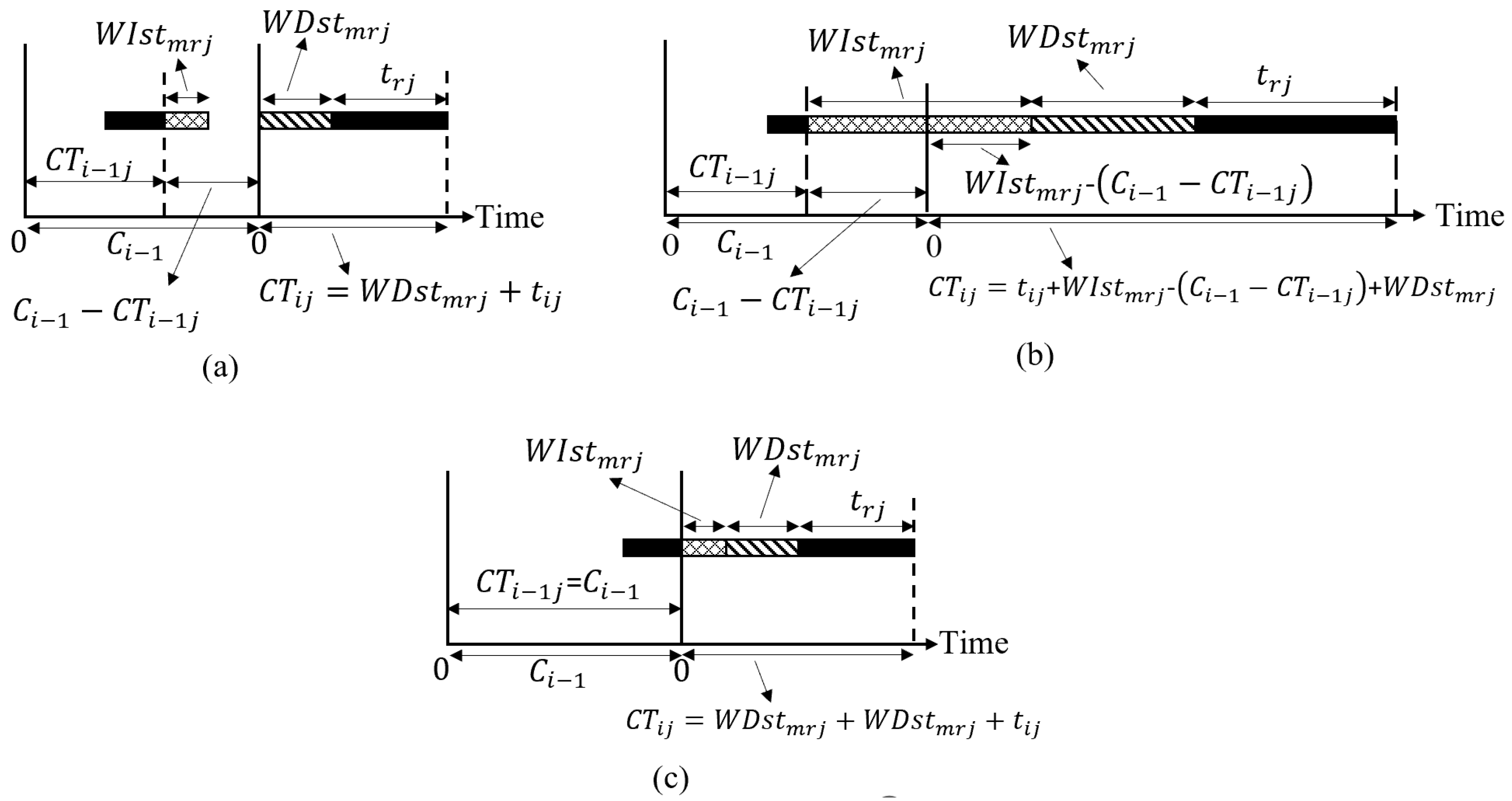
2.2.4. Completion Time

The completion time of the workpiece currently being processed at station j depends on the completion time of the immediately preceding workpiece that was processed at this station. When station j finishes its task, there are two possible cases.
Case 1: At least one station’s operator has not completed their tasks. In this case, station j must wait until all other station operators finish their current tasks. This means C i 1 > C T i 1 j , allowing the operator at station j to start the workpiece-independent part of the setup for the subsequent workpiece.
If C i 1 C T i 1 j W I s t m r j , then the operator can fully complete this setup phase before the next workpiece arrives at the workstation, as depicted in Figure 2a. Consequently, once the workpiece is in place, the operator proceeds with the workpiece-dependent setup activities and then starts working on it. In this context, W D s t m r j + t r j W I s t m r j C i 1 C T i 1 j + W D s t m r j + t r j and
C T i j = m = 1 M r = 1 M X h I + i + 1 j m r W D s t m r j + t r j
If C i 1 C T i 1 j < W I s t m r j , then during the interval between completing their task and the next workpiece entering the workstation, the operator can only complete part of the workpiece-independent setup. The remaining part of the setup must be completed after the respective workpiece arrives at the station, as depicted in Figure 2b. In this scenario, W I s t m r j C i 1 C T i 1 j + W D s t m r j + t r j > W D s t m r j + t r j and
C T i j = m = 1 M r = 1 M X h * I + i + 1 j m r * t r j + W I s t m r j C i 1 C T i 1 j + W D s t m r j
Case 2: all operators at other stations have finished their tasks. In this case, as soon as the operator at station j completes their tasks, the conveyor belt immediately moves each workpiece to the next station, making C i 1 = C T i 1 j . Consequently, the workpiece-independent and workpiece-dependent parts of the setup are carried out only after the workpiece has entered the station, as shown in Figure 2c. Here, W I s t m r j C i 1 C T i 1 j + W D s t m r j + t r j = W I s t m r j + W D s t m r j + t r j and
C T i j = m = 1 M r = 1 M X h I + i + 1 j m r W I s t m r j + W D s t m r j + t r j
Consequently, the constraint of the completion time is
C T i j = max m = 1 M r = 1 M X h * I + i + 1 j m r   * t r j + W D s t m r j ,   m = 1 M r = 1 M X h * I + i + 1 j m r * t r j + W I s t m r j C i 1 C T i 1 j + W D s t m r j f o r   i = 2 , , I   j = 1 , , K

2.2.5. The Interval between Consecutive Movements of the Conveyor Belt

In the synchronous assembly line, the conveyor belt initiates movement once every station finishes its tasks. Consequently, the interval between the current and the next conveyor belt movement matches the maximum task time among the workpieces currently being processed at the stations. Therefore:
C i C T i j   f o r   i = 1 , , I                   f o r   j = 1 , , K
The proposed mathematical model can be written as:
m i n i m i z e i = 1 I C i
          ST
m = 1 M r = 1 M X i m r = 1     f o r     i = 1,2 , , I
i = 1 I m = 1 M X i m r = d r     f o r     r = 1,2 , , M
m = 1 M X i m r = p = 1 M X i + 1 r p     f o r     i = 1,2 , , I 1     f o r     r = 1,2 , , M
m = 1 M X I m r = p = 1 M X 1 r p     f o r     r = 1,2 , , M
C T 1 j = m = 1 M r = 1 M X h + I + 2 j m r W I s t m r j + W D s t m r j + t r j     f o r     h = 0,1 , , K I + 1     f o r     j = m a x h 1 I + i + 1 , 1 , , m i n K , h I + i
C T i j = max m = 1 M r = 1 M X h I + i + 1 j m r W D s t m r j + t r j , m = 1 M r = 1 M X h I + i + 1 j m r W I s t m r j C i 1 C T i 1 j + W D s t m r j + t r j   f o r   i = 2 , , I
f o r   h = 0,1 , , K I + 1   f o r   j = m a x h 1 I + i + 1 , 1 , , K , h I + i C i C T i j   f o r   i = 1 , , I   f o r   j = 1 , , K
The objective function (Equation (10a)) minimizes the sum of launching intervals between workpieces in the assembly line. Constraint (Equation (10b)) ensures that each sequence position is occupied by exactly one product. Constraint (Equation (10c)) confirms that the demand for each model is satisfied within a cycle. Constraints (Equation (10d)) and (Equation (10e)) maintain the product sequence throughout the cyclic production of energy devices. Constraints (Equation (10f)) and (Equation (10g)) compute the completion times for the first and the i-th products in a sequence at station j, respectively. Finally, constraint (Equation (10h)) defines the intervals between consecutive conveyor belt movements. The proposed algorithm demonstrated that this model effectively reduces the overall cycle time of the manufacturing unit, which impacts the integration of different material layers in the final device. As shown in the objective function (Equation (10a)), the proposed algorithm significantly reduces the time required for manufacturing and simultaneously enhances energy efficiency by decreasing the overall cycle time of the manufacturing unit. Reducing cycle time decreases the energy consumption per unit time for operating machines in the manufacturing unit, considering that most machinery units consume substantial energy during ramping up and ramping down.

3. Proposed Algorithm and Mathematical Result

Unlike traditional optimization methods such as simulated annealing and tabu search, which typically focus on refining a single solution, genetic algorithms explore the solution space by maintaining and evolving a population of solutions [77]. Therefore, it increases the likelihood of finding a global optimum by simultaneously investigating multiple regions of the solution space. Given the nonlinear and NP-hard nature of the problem, a metaheuristic algorithm based on GAs has been developed.

3.1. Basic Genetic Algorithm Structure

GAs are intelligent, adaptive search algorithms characterized by flexibility and their probabilistic nature. Despite their randomness, GAs systematically utilize past data to navigate toward areas of improved performance within the search space. They belong to stochastic adaptive search methods that apply Darwinian principles of natural selection, or “survival of the fittest”, to identify optimal solutions. In the process, GA navigates the problem domain, which is composed of chromosomes, selecting those for further exploration based on their performance. Each chromosome represents a potential solution or point within the search space. Through genetic operators, GA generates new, potentially more viable structures (offspring) from those that perform well (parents), ensuring that successful traits are propagated through generations within the population. GAs operate on the following foundational steps:
(1)
Generate the initial population by creating random numbers (chromosomes).
(2)
Determine the fitness value for each chromosome.
(3)
Continue the process until a termination condition is reached:
a.
Select parents from the population.
b.
Apply crossover to the selected parents.
c.
Perform mutations on the chromosomes.
d.
Calculate the fitness value for each new chromosome.
e.
Select the offspring to form the next generation.

3.2. Proposed Genetic Algorithm

In this section, a genetic algorithm is developed to solve problem sizes typical for real business applications.

3.2.1. Initial Population

A set of N chromosomes, representing the population size, is randomly generated. Each chromosome is structured as a sequence of all products that are produced within one cycle.

3.2.2. Selection

A subset of chromosomes is chosen based on fitness values to form the next generation. The selection probability for each chromosome is determined by its fitness value, using a proportional selection method where the probability of a chromosome being selected is proportional to its fitness. Consequently, chromosomes with higher fitness values are more likely to be selected for the subsequent generation. The calculation of the fitness value for each chromosome is outlined as follows:
P i = F m a x F i                   f o r   i = 1,2 , , N
where N represents the population size, F m a x is the largest objective function value in the current population, and F i is the objective function value for the i-th chromosome. In the study by Gillies [78], the power-law scaling ( ) was proposed, which raises the raw fitness to a specific value, enhancing the selection process. Chromosome selection is then carried out using the roulette wheel selection method, where each chromosome’s probability of being chosen is influenced by its adjusted fitness value.

3.2.3. Crossover

Crossover is a genetic operator employed to create superior offspring by combining the genetic information of two chromosomes, referred to as parents. In this paper, the order crossover (OX) [79] was chosen for the proposed genetic algorithm. To demonstrate the OX function, we consider the following example with two parent sequences:
P a r e n t   1 :   A   B   B C   A   A   B   D B   C   B   D   A   C
P a r e n t   2 :   C   B   A B   B   C   A   A D   B   A   C   D   B
Brackets indicate the segments of the sequences that will stay unchanged and be incorporated into the offspring during the crossover process. While the placement of these brackets is random, the left bracket is positioned after the first character of the sequence, and the right bracket before the last character. A new parent sequence is created by relocating all characters appearing after the right bracket (in the original parent) to the start of the sequence. The outcome of this procedure is illustrated below:
P a r e n t   1 :   B   C   B D   A   C   A   B B   C   A   A   B   D   ( D   C   B   B   C   A   A   B   D )
P a r e n t   2 :   D   B   A C   D   B   C   B A   B   B   C   A   A   ( D   B   C   B   B   B   C   A   A )
From this newly formed sequence, characters identical to those found between the brackets in the other original parent are removed (with characters to be removed highlighted in bold). For instance, in Parent 1′, the first two As, the first two Bs, and the first C are removed since Parent 2 contains the sequence BBCAA within its brackets. The sequence found between the brackets in the original parent, combined with the shortened list from the other parent (as indicated in parentheses above), is then used to construct an offspring. For example, the CAABD sequence from Parent 1 and the reduced list from Parent 2′ are combined, starting from the right bracket and continuing to the sequence’s start. This approach yields the following offspring [80]:
O f f s p r i n g   1 :   C   A   A C   A   A   B   D D   B   C   B   B   B
O f f s p r i n g   2 :   A   B   D B   B   C   A   A D   C   B   B   C   A

3.2.4. Inversion

The inversion operator generates offspring from a single parent by selecting two random points within the parent sequence. The elements between these cut points are then inverted. Here is an example illustrating the inversion operator:
B e f o r e   i n v e r s i o n :   C   B   A B   A   B   C C   A
A f t e r   i n v e r s i o n :   C   B   A C   B   A   B C   A

3.2.5. Mutation

Mutation brings diversity into the population by randomly changing chromosomes, preventing the gene pool from becoming homogeneous and reducing the risk of premature convergence. This operator randomly modifies one or more genes in a single parent. In this study, the swapping mutation technique was used. Consider the following sequence:
B e f o r e   m u t a t i o n : D   A   B   A   B _   C   B   A   A   B   C _   A   D   A
The two underlined elements are uniquely and randomly selected for swapping. Following this mutation, the sequence is updated to:
A f t e r   m u t a t i o n : D   A   B   A   C _   C   B   A   A   B   B _   A   D   A

3.3. Numerical Experiment and Discussion

It is challenging to conclude the superiority of one method over the other without knowing the global optimal. The present study used a benchmarking approach as a practical solution to address this issue by comparing the GA’s performance against Lingo’s branch and bound (B&B) method for small-sized problems. The B&B method is commonly applied to integer linear programs and is effective at locating local optimal within nonlinear programming contexts [48]. Therefore, the efficiency of the proposed genetic algorithm is benchmarked against Lingo’s B&B method for solving the model. The rationale was that for small-sized problems, Lingo’s B&B is likely to find the global optimum or a very close approximation, thus providing a reliable benchmark. By comparing the GA’s performance against Lingo’s B&B, if both achieve optimal solutions in these small-sized problems, the study can assess the GA’s effectiveness in finding solutions for large-sized problems in comparison with Lingo’s B&B. The GA was executed on an Intel® Core (TM) i7 CPU (1.9 GHz) with Windows 10 and 16 GB of RAM and programmed using the Visual Fortran language. Two sets of randomly generated MMAL problems were used to evaluate the effectiveness of the proposed GA: small- and large-sized problems. For all test problems, the following assumptions were made:
(1)
The setup times ( S T m r j ) were generated from a uniform distribution of U(4,9), and the setup times ( t r j ) from U(2,4), respectively.
(2)
The parameters for GA, including   N (population size), (the power-law scaling), P c (crossover probability), P i (inversion probability), P m (mutation probability), and I m a x (maximum number of algorithm iterations) were set as 40, 1.005, 0.7, 0.5, 0.1, and 1000, respectively. Parameter setting can follow either offline or online strategies. With offline parameter initialization, the values are set before the meta-heuristic’s execution. However, the online strategy allows parameters to be dynamically or adaptively adjusted during the run. This study utilized the offline method, determining the optimal parameters by solving two test problems—one small-sized and one large-sized—using a set of different parameters. The best-performing parameters were then selected for the proposed GA.
(3)
Each test problem was subjected to ten GA runs.
Table 3 shows the proposed algorithm and the Lingo 19.0 results for small-sized problems.
Problem no: identifier for problem instances; SSPi (i = 1, 2, …, 15): small-sized problems numbered 1 through 15; Size (M, K, I): number of models, stations, and total products, respectively; WIst%: percentage of setup time that is workpiece-independent; OFV: objective function value by Lingo software; CPU time1 (s): computational time taken by Lingo using branch and bound in seconds; f m i n : best solution value from the proposed genetic algorithm over ten runs; CPU time2 (s): average computation time for the proposed genetic algorithm over ten runs, in seconds; c v ^ 2 : squared coefficient of variation for solution consistency; g a p ^ : percentage difference between Lingo’s objective function value (OFV) and the algorithm’s best solution value ( f m i n ).
In Table 3, Column 4 displays the objective function value of the best solution (Best Obj) achieved by the Lingo software. The sixth column highlights the best solution ( f m i n ) achieved from ten runs of the proposed algorithm. The coefficient of variation c v ^ 2 , as proposed by Fattahi, et al. [81], is used to assess the algorithm’s convergence. This index, referred to as the variation rate, is detailed below:
c v ^ 2 = i = 1 10 f i f ¯ 2 n 1 f ¯ 2
where f i represents the objective function value obtained in the i-th run of the GA algorithm and f ¯ is the average of the objective function values from ten runs of the GA algorithm. Additionally, the index g a p ^ is used to evaluate the proposed algorithm’s efficacy in finding quality solutions. This index, calculated using Equation (13), indicates the gap between the best solution derived from Lingo (Best Obj) and the best solution achieved by the proposed algorithm.
g a p ^ = B e s t   O b j f m i n B e s t   O b j × 100
The zero g a p ^ values across all small-sized problems in the last column of Table 3 illustrate that the GA consistently matched the optimal solutions provided by Lingo. Therefore, this demonstrates GA’s effectiveness in matching Lingo’s solution quality. Moreover, the CPU times for the proposed algorithm are notably less than those for the Lingo software, as demonstrated in Table 3. The CPU time for each problem associated with the proposed algorithm represents the average CPU times from ten runs of the GA algorithm. For every problem, the outcome of the index c v ^ 2 indicates that a consistent solution has been achieved across ten proposed algorithm runs. The analysis of results in Table 3 indicates that for small-sized problem instances, the GA was able to find the optimal solutions, the same as Lingo’s B&B, validating its effectiveness in such scenarios. Therefore, the efficiency of the proposed genetic algorithm is benchmarked against Lingo’s B&B method for solving large-sized problems through the model. The outcomes of the experiment on large-sized problems are shown in Table 4.
Problem no: identifier for problem instances; LSPi (i = 1, 2, …, 12): large-sized problems numbered 1 through 12; Size (M, K, I): number of models, stations, and total products, respectively; WIst%: percentage of setup time that is workpiece-independent; Best Obj: best solution found by the Lingo software; g a p I P : percentage difference between Lingo’s best objective value and the objective bound; f m i n : best solution value from the proposed genetic algorithm over ten runs; CPU time (s): average computational time for the proposed genetic algorithm over ten runs, in seconds; c v ^ 2 : squared coefficient of variation for solution consistency; g a p ^ : percentage difference between Lingo’s best solution (Best Obj) and the algorithm’s best solution value ( f m i n ).
Given the complexity of these problems, the Lingo software could not find a satisfactory solution within a reasonable timeframe. Therefore, the results for the Lingo software (shown in Table 4) are based on runs lasting 3600 s. Column 4 in Table 4 shows the best objective identified by the Lingo software. Additionally, column 5 details the gap between the best objective value and the objective bound. The objective bound (Obj bound) represents a limitation on the best possible value the objective can achieve. For large-sized problems, the g a p ^ values highlight the GA’s superior performance, reinforcing its capability to efficiently handle larger and more complex problem sets.
LSPi (i = 1, 2, …, 12): large-sized problems numbered 1 through 12. The markers indicate the actual solutions obtained at the end of a 3600-s run for Lingo’s B&B method (red circles for the best objective and blue circles for the objective bound) and the best solution of the proposed GA (blue circles). Lines connecting the markers are used for illustration purposes only and do not represent additional data points or continuous trends.
In a typical B&B algorithm, the gap between the objective bound and the best objective narrows over time, eventually closing when the optimal solution is found. However, in Figure 3, Lingo’s B&B method did not converge to an optimal solution within the 3600-s cutoff, leaving a gap that indicates the best objective is a likely local optimum rather than the global solution. Figure 4 displays the discrepancy between the best and average solutions derived from ten runs of the proposed GA for large-sized problems.
In Figure 4, the proposed GA demonstrates tight convergence between its best and average solutions, with discrepancies lying within the narrow range of 0.9 to 2.7 for large-sized problems. This low variation suggests a high solution stability and reliability across different runs. The low c v ^ 2 values corroborate the algorithm’s consistency across runs. Figure 4 and the c v ^ 2 index results indicate that the algorithm’s outcomes exhibit very low variation and high convergence.
Table 3 and Table 4 indicate the efficiency of the proposed GA capability in solving sequencing problems for MMSAL with bipartite setups. For small problems, the GA consistently achieves the optimal solution and requires less computational time, demonstrating its capacity to find high-quality solutions more efficiently than the Lingo software, as detailed in Table 3. For larger problems, Lingo’s B&B algorithm struggled to find satisfactory solutions within a reasonable timeframe (3600 s), often resulting in a local optimum. In contrast, the GA demonstrated superior performance, managing the computational complexity within a reasonable time frame and providing solutions with low variation, as shown in Table 4 and Figure 3 and Figure 4. The reasons are:
  • Consistency of solutions: The GA was run multiple times (ten runs) for each problem instance. The low coefficient of variation ( c v ^ 2 )   values indicate that the GA consistently produced similar high-quality solutions across different runs, demonstrating its reliability.
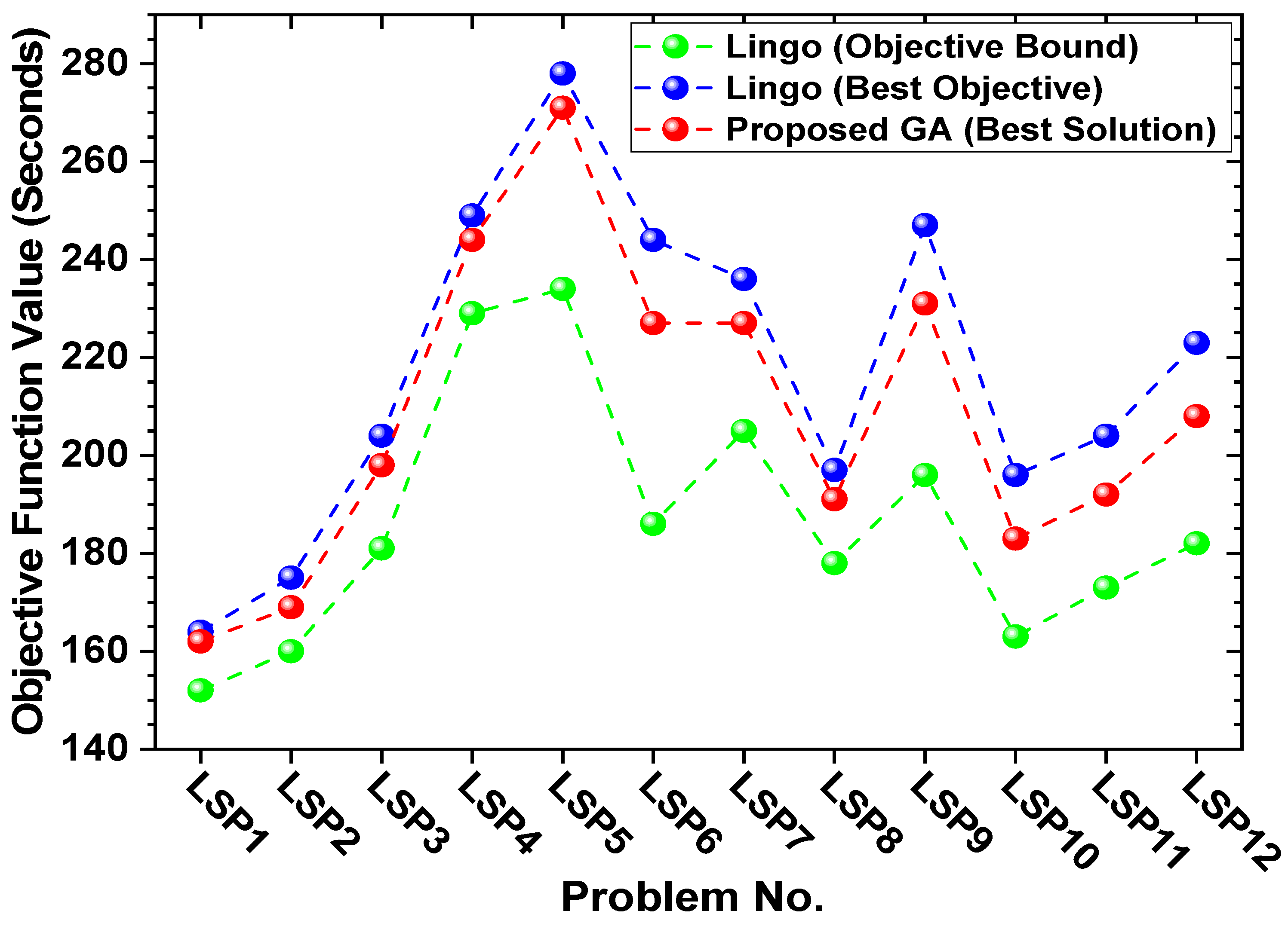
  • Performance metrics: The comparison included the objective function values, computational times, and the convergence characteristics of the GA. The proposed GA showed faster convergence and required less computational time, which is crucial for practical applications.
The results highlight the GA’s viability as a practical and efficient method, particularly in manufacturing lines for energy devices that require fast and reliable sequencing solutions. Even with larger and more complex problems, the GA’s consistent and robust performance supports its application in real-world manufacturing systems for energy devices, where enhancing productivity and responsiveness is paramount.

4. Conclusions

This study introduces an innovative approach to sequence-dependent setup times in unpaced synchronous MMALs by categorizing them into workpiece-independent and -dependent activities. This categorization enhances early task initiation, optimizing assembly operations. A mathematical model is designed to optimize sequencing for these bipartite setup times, minimizing intervals between workpiece launches. Due to the NP-hard nature of the problem, a meta-heuristic GA is used, and its performance with Lingo software is compared across two sets of problem sizes. Determining the global optimum is essential for conclusively comparing methods, which is difficult due to the NP-hard nature of the problem. Therefore, this study used a benchmarking approach to compare the performance of the proposed GA against Lingo’s B&B algorithm to solve the model. For small-sized problems, Lingo’s B&B found the same optimal solutions as the GA, thus providing a reliable benchmark. By comparing the GA’s performance against Lingo’s B&B, which achieved optimal solutions in these small-sized problems, the study assessed the GA’s effectiveness in solving large-sized problems. The GA consistently achieves optimal solutions faster than Lingo for small-sized problems. For large-sized problems, the GA effectively managed complexity within reasonable timeframes, outperforming Lingo software, which fell short of the 3600-s limit. Moreover, the GA’s results highlighted a tight convergence between best and average solutions and low c v ^ 2 values, demonstrating its accuracy and reliability in achieving quality solutions across different runs. By conducting this comparison, the GA achieved comparable or better solutions, particularly for large-sized problems where Lingo struggled due to computational limits and the inherent complexity of the problem. The proposed GA’s ability to manage computational complexity within reasonable time frames and consistent performance underscores its potential for real-world applications in manufacturing lines for energy devices. Future work can study the problems addressed in this paper using different proposed algorithms and compare their results with those of the current study to provide a more comprehensive comparison with the proposed GA. These findings form a foundation for further investigation into bipartite setups in paced assembly lines and cost minimization strategies, thus expanding the model’s applicability and reinforcing its relevance in manufacturing lines of energy devices.

Author Contributions

Conceptualization, A.V. and M.H.G.; Methodology, A.V., M.S. and M.H.G.; Software, A.V. and M.S.; Validation, A.V., M.S. and M.H.G.; Formal analysis, A.V., M.S. and M.H.G.; Investigation, A.V., M.S. and M.H.G.; Data curation, A.V., M.S. and M.H.G.; Writing—original draft, A.V. and M.S.; Writing—review & editing, M.H.G.; Visualization, A.V. and M.S.; Supervision, M.H.G. All authors have read and agreed to the published version of the manuscript.

Funding

This research received no external funding.

Data Availability Statement

The original contributions presented in the study are included in the article, further inquiries can be directed to the corresponding author.

Acknowledgments

M.H.G. acknowledges the Faculty Startup Support from the San Diego State University (SDSU).

Conflicts of Interest

The authors declare no competing interests.

References

  1. Renna, P.; Materi, S. A literature review of energy efficiency and sustainability in manufacturing systems. Appl. Sci. 2021, 11, 7366. [Google Scholar] [CrossRef]
  2. Gielen, D.; Gorini, R.; Wagner, N.; Leme, R.; Gutierrez, L.; Prakash, G.; Asmelash, E.; Janeiro, L.; Gallina, G.; Vale, G.; et al. Global Energy Transformation: A Roadmap to 2050; International Renewable Energy Agency: Masdar City, United Arab Emirates, 2019. [Google Scholar]
  3. Zheng, Y.; Shan, R.; Xu, W.; Qiu, Y. Effectiveness of carbon dioxide emission target is linked to country ambition and education level. Commun. Earth Environ. 2024, 5, 209. [Google Scholar] [CrossRef]
  4. Spence, A.; Leygue, C.; Bedwell, B.; O’Malley, C. Engaging with energy reduction: Does a climate change frame have the potential for achieving broader sustainable behaviour? J. Environ. Psychol. 2014, 38, 17–28. [Google Scholar] [CrossRef]
  5. Akerman, P.; Cazzola, P.; Christiansen, E.S.; Van Heusden, R.; Kolomanska-van Iperen, J.; Christensen, J.; Crone, K.; Dawe, K.; De Smedt, G.; Keynes, A. Reaching Zero with Renewables; International Renewable Energy Agency: Masdar City, United Arab Emirates, 2020. [Google Scholar]
  6. Paprocka, I.; Krenczyk, D. On Energy Consumption and Productivity in a Mixed-Model Assembly Line Sequencing Problem. Energies 2023, 16, 7091. [Google Scholar] [CrossRef]
  7. Gupta, M.K.; Korkmaz, M.E.; Yılmaz, H.; Şirin, Ş.; Ross, N.S.; Jamil, M.; Królczyk, G.M.; Sharma, V.S. Real-time monitoring and measurement of energy characteristics in sustainable machining of titanium alloys. Measurement 2024, 224, 113937. [Google Scholar] [CrossRef]
  8. Baldwin, R.; Freeman, R. Risks and global supply chains: What we know and what we need to know. Annu. Rev. Econ. 2022, 14, 153–180. [Google Scholar] [CrossRef]
  9. Sun, L.; Yuan, G.; Gao, L.; Yang, J.; Chhowalla, M.; Gharahcheshmeh, M.H.; Gleason, K.K.; Choi, Y.S.; Hong, B.H.; Liu, Z. Chemical vapour deposition. Nat. Rev. Methods Prim. 2021, 1, 5. [Google Scholar] [CrossRef]
  10. Heydari Gharahcheshmeh, M.; Gleason, K.K. Device fabrication based on oxidative chemical vapor deposition (oCVD) synthesis of conducting polymers and related conjugated organic materials. Adv. Mater. Interfaces 2019, 6, 1801564. [Google Scholar] [CrossRef]
  11. Chowdhury, K.; Behura, S.K.; Rahimi, M.; Heydari Gharahcheshmeh, M. oCVD PEDOT-Cl Thin Film Fabricated by SbCl5 Oxidant as the Hole Transport Layer to Enhance the Perovskite Solar Cell Device Stability. ACS Appl. Energy Mater. 2024, 7, 1068–1079. [Google Scholar] [CrossRef]
  12. Sun, Y.; Rogers, J.A. Inorganic semiconductors for flexible electronics. Adv. Mater. 2007, 19, 1897–1916. [Google Scholar] [CrossRef]
  13. Heydari Gharahcheshmeh, M.; Tavakoli, M.M.; Gleason, E.F.; Robinson, M.T.; Kong, J.; Gleason, K.K. Tuning, optimization, and perovskite solar cell device integration of ultrathin poly (3,4-ethylene dioxythiophene) films via a single-step all-dry process. Sci. Adv. 2019, 5, eaay0414. [Google Scholar] [CrossRef] [PubMed]
  14. Heydari Gharahcheshmeh, M.; Gleason, K.K. Recent Progress in Conjugated Conducting and Semiconducting Polymers for Energy Devices. Energies 2022, 15, 3661. [Google Scholar] [CrossRef]
  15. Gharahcheshmeh, M.H.; Gleason, K.K. Conjugated polymers for flexible energy harvesting and storage devices. In Conjugated Polymers for Next-Generation Applications; Elsevier: Amsterdam, The Netherlands, 2022; pp. 283–311. [Google Scholar]
  16. Gleason, K.K.; Gharahcheshmeh, M.H. Conjugated Polymers at Nanoscale: Engineering Orientation, Nanostructure, and Properties; Walter de Gruyter GmbH & Co KG: Berlin, Germany, 2021. [Google Scholar]
  17. Tavakoli, M.M.; Gharahcheshmeh, M.H.; Moody, N.; Bawendi, M.G.; Gleason, K.K.; Kong, J. Efficient, Flexible, and Ultra-Lightweight Inverted PbS Quantum Dots Solar Cells on All-CVD-Growth of Parylene/Graphene/oCVD PEDOT Substrate with High Power-per-Weight. Adv. Mater. Interfaces 2020, 7, 2000498. [Google Scholar] [CrossRef]
  18. Heydari Gharahcheshmeh, M.; Chowdhury, K. Enhancing Capacitance of Carbon Cloth Electrodes via Highly Conformal PEDOT Coating Fabricated by the OCVD Method Utilizing SbCl5 Oxidant. Adv. Mater. Interfaces 2024, 2400118. [Google Scholar] [CrossRef]
  19. Heydari Gharahcheshmeh, M.; Robinson, M.T.; Gleason, E.F.; Gleason, K.K. Optimizing the optoelectronic properties of face-on oriented poly (3,4-ethylenedioxythiophene) via water-assisted oxidative chemical vapor deposition. Adv. Funct. Mater. 2021, 31, 2008712. [Google Scholar] [CrossRef]
  20. Pilati, F.; Lelli, G.; Regattieri, A.; Ferrari, E. Assembly line balancing and activity scheduling for customised products manufacturing. Int. J. Adv. Manuf. Technol. 2022, 120, 3925–3946. [Google Scholar] [CrossRef]
  21. Akpinar, S.; Bayhan, G.M. Performance evaluation of ant colony optimization-based solution strategies on the mixed-model assembly line balancing problem. Eng. Optim. 2014, 46, 842–862. [Google Scholar] [CrossRef]
  22. Bortolini, M.; Ferrari, E.; Gamberi, M.; Pilati, F.; Faccio, M. Assembly system design in the Industry 4.0 era: A general framework. Ifac-Papersonline 2017, 50, 5700–5705. [Google Scholar] [CrossRef]
  23. Kim, S.H.; Lee, Y.H. Synchronized production planning and scheduling in semiconductor fabrication. Comput. Ind. Eng. 2016, 96, 72–85. [Google Scholar] [CrossRef]
  24. Liu, Q.; Wang, W.-x.; Zhu, K.-r.; Zhang, C.-y.; Rao, Y.-q. Advanced scatter search approach and its application in a sequencing problem of mixed-model assembly lines in a case company. Eng. Optim. 2014, 46, 1485–1500. [Google Scholar] [CrossRef]
  25. Buzacott, J.A.; Shanthikumar, J.G. Stochastic Models of Manufacturing Systems; Prentice Hall: Upper Saddle River, NJ, USA, 1993. [Google Scholar]
  26. Lin, L.; Drury, C.; Kim, S.W. Ergonomics and quality in paced assembly lines. Hum. Factors Ergon. Manuf. Serv. Ind. 2001, 11, 377–382. [Google Scholar] [CrossRef]
  27. Chiang, W.-C.; Urban, T.L.; Xu, X. A bi-objective metaheuristic approach to unpaced synchronous production line-balancing problems. Int. J. Prod. Res. 2012, 50, 293–306. [Google Scholar] [CrossRef]
  28. Bard, J.F.; Dar-Elj, E.; Shtub, A. An analytic framework for sequencing mixed model assembly lines. Int. J. Prod. Res. 1992, 30, 35–48. [Google Scholar] [CrossRef]
  29. Rauf, M.; Guan, Z.; Sarfraz, S.; Mumtaz, J.; Shehab, E.; Jahanzaib, M.; Hanif, M. A smart algorithm for multi-criteria optimization of model sequencing problem in assembly lines. Robot. Comput.-Integr. Manuf. 2020, 61, 101844. [Google Scholar] [CrossRef]
  30. Mosadegh, H.; Ghomi, S.F.; Süer, G.A. Stochastic mixed-model assembly line sequencing problem: Mathematical modeling and Q-learning based simulated annealing hyper-heuristics. Eur. J. Oper. Res. 2020, 282, 530–544. [Google Scholar] [CrossRef]
  31. Emde, S.; Polten, L. Sequencing assembly lines to facilitate synchronized just-in-time part supply. J. Sched. 2019, 22, 607–621. [Google Scholar] [CrossRef]
  32. Aroui, K.; Alpan, G.; Frein, Y. Minimising work overload in mixed-model assembly lines with different types of operators: A case study from the truck industry. Int. J. Prod. Res. 2017, 55, 6305–6326. [Google Scholar] [CrossRef]
  33. Mosadegh, H.; Fatemi Ghomi, S.; Süer, G.A. Heuristic approaches for mixed-model sequencing problem with stochastic processing times. Int. J. Prod. Res. 2017, 55, 2857–2880. [Google Scholar] [CrossRef]
  34. Fattahi, P.; Beitollahi Tavakoli, N.; Fathollah, M.; Roshani, A.; Salehi, M. Sequencing mixed-model assembly lines by considering feeding lines. Int. J. Adv. Manuf. Technol. 2012, 61, 677–690. [Google Scholar] [CrossRef]
  35. Fattahi, P.; Salehi, M. Sequencing the mixed-model assembly line to minimize the total utility and idle costs with variable launching interval. Int. J. Adv. Manuf. Technol. 2009, 45, 987–998. [Google Scholar] [CrossRef]
  36. Kim, S.; Jeong, B. Product sequencing problem in Mixed-Model Assembly Line to minimize unfinished works. Comput. Ind. Eng. 2007, 53, 206–214. [Google Scholar] [CrossRef]
  37. Sarker, B.R.; Pan, H. Designing a mixed-model assembly line to minimize the costs of idle and utility times. Comput. Ind. Eng. 1998, 34, 609–628. [Google Scholar] [CrossRef]
  38. Bolat, A. Stochastic procedures for scheduling minimum job sets on mixed model assembly lines. J. Oper. Res. Soc. 1997, 48, 490–501. [Google Scholar] [CrossRef]
  39. Xiaobo, Z.; Ohno, K. Algorithms for sequencing mixed models on an assembly line in a JIT production system. Comput. Ind. Eng. 1997, 32, 47–56. [Google Scholar] [CrossRef]
  40. Xiaobo, Z.; Ohno, K. A sequencing problem for a mixed-model assembly line in a JIT production system. Comput. Ind. Eng. 1994, 27, 71–74. [Google Scholar] [CrossRef]
  41. Yano, C.A.; Rachamadugu, R. Sequencing to minimize work overload in assembly lines with product options. Manag. Sci. 1991, 37, 572–586. [Google Scholar] [CrossRef]
  42. Bard, J.; Shtub, A.; Joshi, S.B. Sequencing mixed-model assembly lines to level parts usage and minimize line length. Int. J. Prod. Res. 1994, 32, 2431–2454. [Google Scholar] [CrossRef]
  43. Rahimi-Vahed, A.R.; Rabbani, M.; Tavakkoli-Moghaddam, R.; Torabi, S.A.; Jolai, F. A multi-objective scatter search for a mixed-model assembly line sequencing problem. Adv. Eng. Inform. 2007, 21, 85–99. [Google Scholar] [CrossRef]
  44. Rahimi-Vahed, A.; Mirzaei, A.H. A hybrid multi-objective shuffled frog-leaping algorithm for a mixed-model assembly line sequencing problem. Comput. Ind. Eng. 2007, 53, 642–666. [Google Scholar] [CrossRef]
  45. Tavakkoli-Moghaddam, R.; Rahimi-Vahed, A. Multi-criteria sequencing problem for a mixed-model assembly line in a JIT production system. Appl. Math. Comput. 2006, 181, 1471–1481. [Google Scholar] [CrossRef]
  46. Giard, V.; Jeunet, J. Optimal sequencing of mixed models with sequence-dependent setups and utility workers on an assembly line. Int. J. Prod. Econ. 2010, 123, 290–300. [Google Scholar] [CrossRef]
  47. Chutima, P.; Naruemitwong, W. A Pareto biogeography-based optimisation for multi-objective two-sided assembly line sequencing problems with a learning effect. Comput. Ind. Eng. 2014, 69, 89–104. [Google Scholar] [CrossRef]
  48. Varyani, A.; Jalilvand-Nejad, A.; Fattahi, P. Determining the optimum production quantity in three-echelon production system with stochastic demand. Int. J. Adv. Manuf. Technol. 2014, 72, 119–133. [Google Scholar] [CrossRef]
  49. Kouvelis, P.; Karabati, S. Cyclic scheduling in synchronous production lines. IIE Trans. 1999, 31, 709–719. [Google Scholar] [CrossRef]
  50. Salehi, M.; Fattahi, P.; Roshani, A.; Zahiri, J. Multi-criteria sequencing problem in mixed-model synchronous assembly lines. Int. J. Adv. Manuf. Technol. 2013, 67, 983–993. [Google Scholar] [CrossRef]
  51. Karabati, S.; Tan, B. Stochastic cyclic scheduling problem in synchronous assembly and production lines. J. Oper. Res. Soc. 1998, 49, 1173–1187. [Google Scholar] [CrossRef]
  52. Oliveira, C.; Lima, T.M. Setup Time Reduction of an Automotive Parts Assembly Line Using Lean Tools and Quality Tools. Eng 2023, 4, 2352–2362. [Google Scholar] [CrossRef]
  53. Lopes, T.C.; Michels, A.S.; Brauner, N.; Magatão, L. Balancing-sequencing paced assembly lines: A multi-objective mixed-integer linear case study. Int. J. Prod. Res. 2023, 61, 5901–5917. [Google Scholar] [CrossRef]
  54. McMullen, P.R.; Tarasewich, P. A beam search heuristic method for mixed-model scheduling with setups. Int. J. Prod. Econ. 2005, 96, 273–283. [Google Scholar] [CrossRef]
  55. Özcan, U. Balancing and scheduling tasks in parallel assembly lines with sequence-dependent setup times. Int. J. Prod. Econ. 2019, 213, 81–96. [Google Scholar] [CrossRef]
  56. Yang, W.; Cheng, W. Modelling and solving mixed-model two-sided assembly line balancing problem with sequence-dependent setup time. Int. J. Prod. Res. 2020, 58, 6638–6659. [Google Scholar] [CrossRef]
  57. Chang, P.-C.; Hsieh, J.-C.; Wang, Y.-W. Genetic algorithms applied in BOPP film scheduling problems: Minimizing total absolute deviation and setup times. Appl. Soft Comput. 2003, 3, 139–148. [Google Scholar] [CrossRef]
  58. Kim, D.-W.; Kim, K.-H.; Jang, W.; Chen, F.F. Unrelated parallel machine scheduling with setup times using simulated annealing. Robot. Comput.-Integr. Manuf. 2002, 18, 223–231. [Google Scholar] [CrossRef]
  59. Schaller, J.E.; Gupta, J.N.; Vakharia, A.J. Scheduling a flowline manufacturing cell with sequence dependent family setup times. Eur. J. Oper. Res. 2000, 125, 324–339. [Google Scholar] [CrossRef]
  60. Laguna, M. A heuristic for production scheduling and inventory control in the presence of sequence-dependent setup times. IIE Trans. 1999, 31, 125–134. [Google Scholar] [CrossRef]
  61. Allahverdi, A.; Soroush, H. The significance of reducing changeover times/changeover costs. Eur. J. Oper. Res. 2008, 187, 978–984. [Google Scholar] [CrossRef]
  62. Akgündüz, O.S.; Tunalı, S. A review of the current applications of genetic algorithms in mixed-model assembly line sequencing. Int. J. Prod. Res. 2011, 49, 4483–4503. [Google Scholar] [CrossRef]
  63. Aslan, Ş. Mathematical model and a variable neighborhood search algorithm for mixed-model robotic two-sided assembly line balancing problems with sequence-dependent setup times. Optim. Eng. 2023, 24, 989–1016. [Google Scholar] [CrossRef]
  64. McMullen, P.R. JIT sequencing for mixed-model assembly lines with setups using tabu search. Prod. Plan. Control 1998, 9, 504–510. [Google Scholar] [CrossRef]
  65. Drexl, A.; Kimms, A. Sequencing JIT mixed-model assembly lines under station-load and part-usage constraints. Manag. Sci. 2001, 47, 480–491. [Google Scholar] [CrossRef]
  66. Boysen, N.; Fliedner, M.; Scholl, A. Sequencing mixed-model assembly lines to minimize part inventory cost. Or Spectr. 2008, 30, 611–633. [Google Scholar] [CrossRef]
  67. Defersha, F.M.; Mohebalizadehgashti, F. Simultaneous balancing, sequencing, and workstation planning for a mixed model manual assembly line using hybrid genetic algorithm. Comput. Ind. Eng. 2018, 119, 370–387. [Google Scholar] [CrossRef]
  68. Zhang, B.; Xu, L.; Zhang, J. A multi-objective cellular genetic algorithm for energy-oriented balancing and sequencing problem of mixed-model assembly line. J. Clean. Prod. 2020, 244, 118845. [Google Scholar] [CrossRef]
  69. Huang, Y.D.; Bian, R.H.; Xu, Z. Sequencing mixed model assembly lines based on genetic algorithm optimization. Adv. Mater. Res. 2011, 279, 412–417. [Google Scholar] [CrossRef]
  70. Monden, Y. Toyota Production System. An Integrated Apprpach to Just-In-Time; Springer: Berlin/Heidelberg, Germany, 1983. [Google Scholar]
  71. Wang, B.G. Sequencing mixed-model assembly lines to minimize the variation of parts consumption by hybrid genetic algorithms. Adv. Mater. Res. 2012, 566, 253–256. [Google Scholar] [CrossRef]
  72. uz Zaman, U.K.; Baqai, A.A. Mixed Model Assembly Line Sequencing by Minimizing Utility Work and Using Genetic Algorithm. In Proceedings of the ASME International Mechanical Engineering Congress and Exposition, Montreal, QC, Canada, 14–20 November 2014; p. V011T014A030. [Google Scholar]
  73. Özcan, U.; Kellegöz, T.; Toklu, B. A genetic algorithm for the stochastic mixed-model U-line balancing and sequencing problem. Int. J. Prod. Res. 2011, 49, 1605–1626. [Google Scholar] [CrossRef]
  74. Moradi, H.; Zandieh, M.; Mahdavi, I. Non-dominated ranked genetic algorithm for a multi-objective mixed-model assembly line sequencing problem. Int. J. Prod. Res. 2011, 49, 3479–3499. [Google Scholar] [CrossRef]
  75. Erel, E.; Gocgun, Y.; Sabuncuoğlu, İ. Mixed-model assembly line sequencing using beam search. Int. J. Prod. Res. 2007, 45, 5265–5284. [Google Scholar] [CrossRef]
  76. Alpay, Ş. GRASP with path relinking for a multiple objective sequencing problem for a mixed-model assembly line. Int. J. Prod. Res. 2009, 47, 6001–6017. [Google Scholar] [CrossRef]
  77. Ponnambalam, S.; Aravindan, P.; Rao, M.S. Genetic algorithms for sequencing problems in mixed model assembly lines. Comput. Ind. Eng. 2003, 45, 669–690. [Google Scholar] [CrossRef]
  78. Gillies, A.M. Machine Learning Procedures for Generating Image Domain Feature Detectors; University of Michigan: Ann Arbor, MI, USA, 1985. [Google Scholar]
  79. Michalewicz, Z. GAs: Why Do They Work? In Genetic Algorithms + Data Structures = Evolution Programs; Springer: Berlin/Heidelberg, Germany, 1996; pp. 45–55. [Google Scholar]
  80. Mansouri, S.A. A multi-objective genetic algorithm for mixed-model sequencing on JIT assembly lines. Eur. J. Oper. Res. 2005, 167, 696–716. [Google Scholar] [CrossRef]
  81. Fattahi, P.; Jolai, F.; Arkat, J. Flexible job shop scheduling with overlapping in operations. Appl. Math. Model. 2009, 33, 3076–3087. [Google Scholar] [CrossRef]
Figure 1. Illustration of workpiece positioning and sequencing on an MMSAL problem with bipartite setups. Ci (i = 1, 2, …, 5): launching interval between workpieces i and i − 1 in a sequence, Symbols (circle, triangle, and pentagon): different product models, Number in symbols (1, 2, …, 5): sequence of five workpieces through the cycles. (a) Detailed illustration of Ci calculation. (b) Detailed illustration of C1 calculation (c) Detailed illustration of C2 calculation.
Energies 17 02865 g001
Figure 2. Illustration of computing completion times under different operational scenarios: (a,b) demonstrate Case 1, where operators start workpiece-independent setup during waiting periods. In (a), there is complete execution of workpiece-independent setup activities before the workpiece’s arrival when time allows, while (b) shows partial execution due to time constraints before the workpiece enters the station. (c) represents Case 2, conducting all setup activities post the workpiece’s entry into the station, triggered by synchronized task completion across stations. See Table 2 for notation details.
Energies 17 02865 g002
Figure 3. Comparison of setup times for Lingo and the proposed GA for large-sized problems.
Energies 17 02865 g003
Figure 4. Discrepancy in total setup time between the best and average solutions of the GA for large-sized problems. The plot exhibits the discrepancy between the best and average solutions derived from ten runs of the proposed GA for the large-sized problems.
Energies 17 02865 g004
Table 1. Calculation of launch intervals for workpiece sequencing in MMSAL.
No. of ProductsStation #1Station #2Station #KLaunch Interval (Ci)
1 P [ I ] P [ I 1 ] P [ I + 1 K ] C 1 = m a x C T P [ I ] 1 , C T P [ I 1 ] 2 , , C T P [ I + 1 K ] K
2 P [ 1 ] P [ I ] P [ I + 1 K 1 ] C 2 = m a x C T P [ 1 ] 1 , C T P [ I ] 2 , , C T P [ I + 1 ( K 1 ) ] K
I P [ I 1 ] P [ I 2 ] P [ I + 1 ( K ( I 1 ) ) ] C I = m a x C T P [ I 1 ] 1 , C T P [ I 2 ] 2 , , C T P [ I + 1 ( K I 1 ) ] K
Table 2. Notation used in the mathematical model.
Indices
i p r o d u c t ,   i 1,2 , , I
j s t a t i o n ,   j 1,2 , , K
m , r m o d e l ,   m , r 1,2 , , M
Input parameters
M N u m b e r   o f   m o d e l s   i n   m i n i m a l   p a r t   s e t
I T o t a l   n u m b e r   o f p r o d u c t s   t o   b e   s e q u e n c e d
K N u m b e r   o f   s t a t i o n
d m N u m b e r   o f   m o d e l s   i n   m i n i m a l   p a r t   s e t
t r j A s s e m b l y   t i m e   f o r m   o d e l   m r 1 ,   , M   a t   j t h   s t a t i o n   ( j 1 ,   , K )
s t m r j T h e   s e t u p   t i m e   r e q u i r e d   w h e n   t h e   m o d e l   t y p e   i s   c h a n g e d   f r o m  
m   t o   r m , r 1 ,   , M   a t   s t a t i o n   j   j 1 ,   , K
W I s t m r j The time required to perform the workpiece-independent part of the setup
W D s t m r j The time required to perform the workpiece-dependent part of the setup
Decision variables
X i m r One ,   if   products   i   and   i + 1     in   a   sequence   are   model   m   and   r , respectively, 0 otherwise
C T i j C o m p l e t i o n   t i m e   o f   p r o d u c t   i   i n   a   s e q u e n c e   a t   s t a t i o n   j
C i T h e   l a u n c h i n g   i n t e r v a l   b e t w e e n   p r o d u c t s   i   a n d   i 1   i n   a   s e q u e n c e
Table 3. Summary of results for small-sized problems.
Problem InformationResult of Lingo Software Using B&BResult of the Proposed GA g a p ^ (%)
Problem No.(M, K, I)WIst = %STOFVCPU
Time1 (s)
f m i n CPU
Time2 (s)
c v ^ 2
SSP13, 3, 1270100.658100.6600
SSP23, 5, 103079.58779.5700
SSP33, 5, 1530114.3581114.31100
SSP43, 5, 1570140.9235140.91200
SSP53, 6, 1040848284900
SSP63, 6, 1340103.6281103.61200
SSP73, 6, 14401376171371300
SSP83, 10, 104095.253995.21400
SSP93, 10, 1560141.81165141.82200
SSP104, 3, 1250112.5123112.5600
SSP114, 3, 1550121.5395121.5800
SSP124, 4, 1050996199600
SSP134, 4, 1230105.6171105.6700
SSP144, 5, 104090.644190.6700
SSP155, 5, 1060939393800
Table 4. Summary of results for large-sized problems.
Problem InformationResult of Lingo Software Using B&BResult of the Proposed GA g a p ^ (%)
Problem No.(M, K, I)WIst = %STBest
Obj (after 3600 s)
g a p I P (%) f m i n CPU Time (s) c v ^ 2
LSP15, 10, 1740167.28.07162.1220.000023.05
LSP25, 10, 1860175.48.04169.5230.000043.36
LSP35, 10, 2040205.411.54193.8260.000045.65
LSP45, 10, 25502508.04241.9320.000083.24
LSP55, 10, 3050277.514.81269.5390.000042.88
LSP66, 8, 2570245.824.08226260.000028.06
LSP76, 10, 2560234.612.57227.7320.000032.94
LSP87, 8, 20501968.63190.2210.000122.96
LSP97, 8, 255024920.32228.6270.000038.19
LSP1010, 8, 2060196.416.65185.1220.000065.75
LSP1110, 10, 2040204.415.41188.5270.000047.78
LSP1210, 12, 203022418.21201.1320.0000310.22
Disclaimer/Publisher’s Note: The statements, opinions and data contained in all publications are solely those of the individual author(s) and contributor(s) and not of MDPI and/or the editor(s). MDPI and/or the editor(s) disclaim responsibility for any injury to people or property resulting from any ideas, methods, instructions or products referred to in the content.

