A Multiscale Hybrid Wind Power Prediction Model Based on Least Squares Support Vector Regression–Regularized Extreme Learning Machine–Multi-Head Attention–Bidirectional Gated Recurrent Unit and Data Decomposition

Abstract

Ensuring the accuracy of wind power prediction is paramount for the reliable and stable operation of power systems. This study introduces a novel approach aimed at enhancing the precision of wind power prediction through the development of a multiscale hybrid model. This model integrates advanced methodologies including Improved Intrinsic Mode Function with Ensemble Empirical Mode Decomposition with Adaptive Noise (ICEEMDAN), permutation entropy (PE), Least Squares Support Vector Regression (LSSVR), Regularized Extreme Learning Machine (RELM), multi-head attention (MHA), and Bidirectional Gated Recurrent Unit (BiGRU). Firstly, the ICEEMDAN technique is employed to decompose the non-stationary raw wind power data into multiple relatively stable sub-modes, while concurrently utilizing PE to assess the complexity of each sub-mode. Secondly, the dataset is reconstituted into three distinct components as follows: high-frequency, mid-frequency, and low-frequency, to alleviate data complexity. Following this, the LSSVR, RELM, and MHA-BiGRU models are individually applied to predict the high-, mid-, and low-frequency components, respectively. Thirdly, the parameters of the low-frequency prediction model are optimized utilizing the Dung Beetle Optimizer (DBO) algorithm. Ultimately, the predicted results of each component are aggregated to derive the final prediction. The empirical findings illustrate the exceptional predictive performance of the multiscale hybrid model incorporating LSSVR, RELM, and MHA-BiGRU. In comparison with other benchmark models, the proposed model exhibits a reduction in Root Mean Squared Error (RMSE) values of over 10%, conclusively affirming its superior predictive accuracy.

1. Introduction

Wind energy is an environmentally friendly and economically viable form of renewable energy. According to the Global Wind Energy Council (GWEC)’s Global Wind Report 2023, global onshore wind power capacity is projected to exceed 100 GW for the first time by 2024 [1]. However, wind energy data exhibit significant randomness and non-stationarity, which has a substantial impact on the stable operation of power systems. Therefore, accurate prediction of wind power is crucial [2,3,4].

Currently, wind energy forecasting methods are mainly divided into physical models, statistical models, and artificial intelligence models [5]. Physical models primarily consider various sources of geographical information, essentially based on Numerical Weather Prediction (NWP) [6] and high-precision wind farm simulation strategies. This approach has been widely applied in countries such as Spain, Denmark, and Germany, with examples including the SOWIE model developed by Eurowind in Germany [7] and a wind sequence correction algorithm based on NWP proposed by Wang et al. [8]. These algorithms utilize large amounts of data to calculate accurate and reliable wind power predictions. However, because of the large data scale, physical models suffer from slow computational speed and low efficiency and are affected by adverse wind farm conditions, making reliable data collection difficult. Statistical methods, on the other hand, do not consider external conditions such as geography or electrical factors. Their core principle uses the relationships between historical wind power data for prediction in order to improve prediction efficiency [9]. Classical models such as Moving Average (MA) [10] and Autoregressive Integrated Moving Average (ARIMA) [11] are based on modeling linear relationships among data. However, when facing complex patterns, these methods suffer from issues of low prediction accuracy and poor performance.

In comparison with the aforementioned approaches, artificial intelligence models have exhibited increasingly remarkable performance in the domain of wind energy prediction. Methods such as Support Vector Regression (SVR) [12], Extreme Learning Machine (ELM) [13], and Gated Recurrent Unit (GRU) [14] have yielded significant accomplishments in wind energy prediction research. However, because of the considerable prediction errors commonly associated with individual models, hybrid prediction models have gained widespread adoption in recent years. Presently, hybrid models primarily encompass the following three facets: data preprocessing, optimization algorithm tuning, and the prediction of single or combined models. Wang et al. [15] optimized the input weights of ELM using genetic algorithms, whereas Zhai, Ma, and Tan [16,17] utilized the Artificial Fish Swarm Algorithm and Salp Swarm Algorithm to optimize the initial input weights and thresholds of ELM. Their outcomes indicate that these models manifest high prediction accuracy. In recent years, the wind power prediction domain has begun embracing deep learning models such as Long Short-Term Memory (LSTM) [18,19], Temporal Convolutional Neural Network (TCN), and Bidirectional Gated Recurrent Unit (BiGRU) [20]. These models and their derivatives have emerged as principal tools in this sphere. Scholars like W. Wang proposed a prediction methodology based on the fusion of TCN and Light Gradient Boosting Machine (LightGBM) [21]. Researchers such as Chi [22] integrated the attention mechanism into the BiGRU-TCN hybrid model and employed wavelet denoising (WT) processed raw data for prediction. Experimental results corroborate the robust predictive capability of this model. Presently, researchers generally favor hybrid models grounded in intelligent algorithms. Zhang et al. [23] proposed a sparse search algorithm (SSA) to optimize the TCN-BiGRU model and employed the Variational Mode Decomposition (VMD) algorithm to decompose data, thereby mitigating the non-stationarity of wind power data. Ablation experiments demonstrated that this model achieved heightened prediction accuracy compared with scenarios where the SSA algorithm was not employed for parameter optimization. The research by the aforementioned scholars underscores that hybrid models, predicated on algorithmic parameter optimization, can further enhance model prediction accuracy.

Wind power data are inherently characterized by randomness and non-stationarity, necessitating data preprocessing to mitigate prediction errors effectively. To address this, scholars have proposed methodologies grounded in signal decomposition for model formulation. For instance, Gao et al. [24] introduced a composite model combining Empirical Mode Decomposition (EMD) with GRU for prediction tasks. However, the EMD algorithm encounters notable challenges such as mode mixing when confronted with gapped signals. In response, scholars have advocated for the incorporation of uniformly distributed white noise into EMD, manifesting as Ensemble Empirical Mode Decomposition (EEMD) and Complementary Ensemble Empirical Mode Decomposition (CEEMD). This technique has found widespread adoption within the prediction domain. For instance, Torres et al. [25] argued that inadequate decomposition processing frequencies may lead to the persistence of white noise’s influence and the emergence of pseudo-mode phenomena. Consequently, they proposed Complementary Ensemble Empirical Mode Decomposition with Adaptive Noise (CEEMDAN), effectively mitigating residual white noise’s impact. Addressing residual noise and pseudo-mode concerns further, Colominas et al. [26] introduced Improved Complementary Ensemble Empirical Mode Decomposition with Adaptive Noise (ICEEMDAN), demonstrating heightened reconstruction accuracy for components and enhanced suitability for nonlinear signal analysis.

In summary, several limitations persist within the realm of wind power prediction. Firstly, prevalent approaches tend to employ single-scale prediction models for all decomposed sub-modes, overlooking the distinctive characteristics of sub-modes across varying frequencies. Secondly, contemporary artificial intelligence prediction methods often encounter challenges in parameter optimization, resulting in high trial and error costs. Lastly, some conventional optimization algorithms exhibit insufficient optimization capabilities and sluggish convergence speeds. Therefore, this paper advocates for a multi-faceted approach by merging data decomposition techniques with multiple models and harnessing the Differential Bees Optimization algorithm (DBO) [27]. This strategy rectifies the existing wind power model shortcomings by addressing deficiencies in sub-mode prediction methods, parameter optimization, and scale singularity.

The main contributions of this paper are as follows:

(1)

This paper proposed a multiscale wind power prediction hybrid model combining data decomposition, LSSVR, RELM, and MHA-BiGRU.

(2)

This paper introduced the ICEEMDAN and PE methods to process the original wind energy series. These methods can effectively address mode mixing and residual noise, thereby better handling the nonlinear and non-stationary characteristics of wind power series.

(3)

This paper introduced the multi-head attention mechanism in the prediction of low-frequency signals, utilizing its strong ability to capture inter-data correlations. Combined with the BiGRU model, this mechanism avoids information loss.

(4)

This paper introduced the DBO optimization algorithm to optimize four parameters including the learning rate, the number of BiGRU neurons, the number of heads in multi-head attention, and the number of filters and regularization parameters. This addresses the limitations and arbitrariness of manual tuning when the MHA-BiGRU model has too many parameters.

(5)

This paper considered the characteristics of information in different frequency bands, used different applicable models, and summed up the results to achieve multiscale hybrid prediction. This overcomes the limitation of insufficient prediction accuracy of a single model.

2. Methods

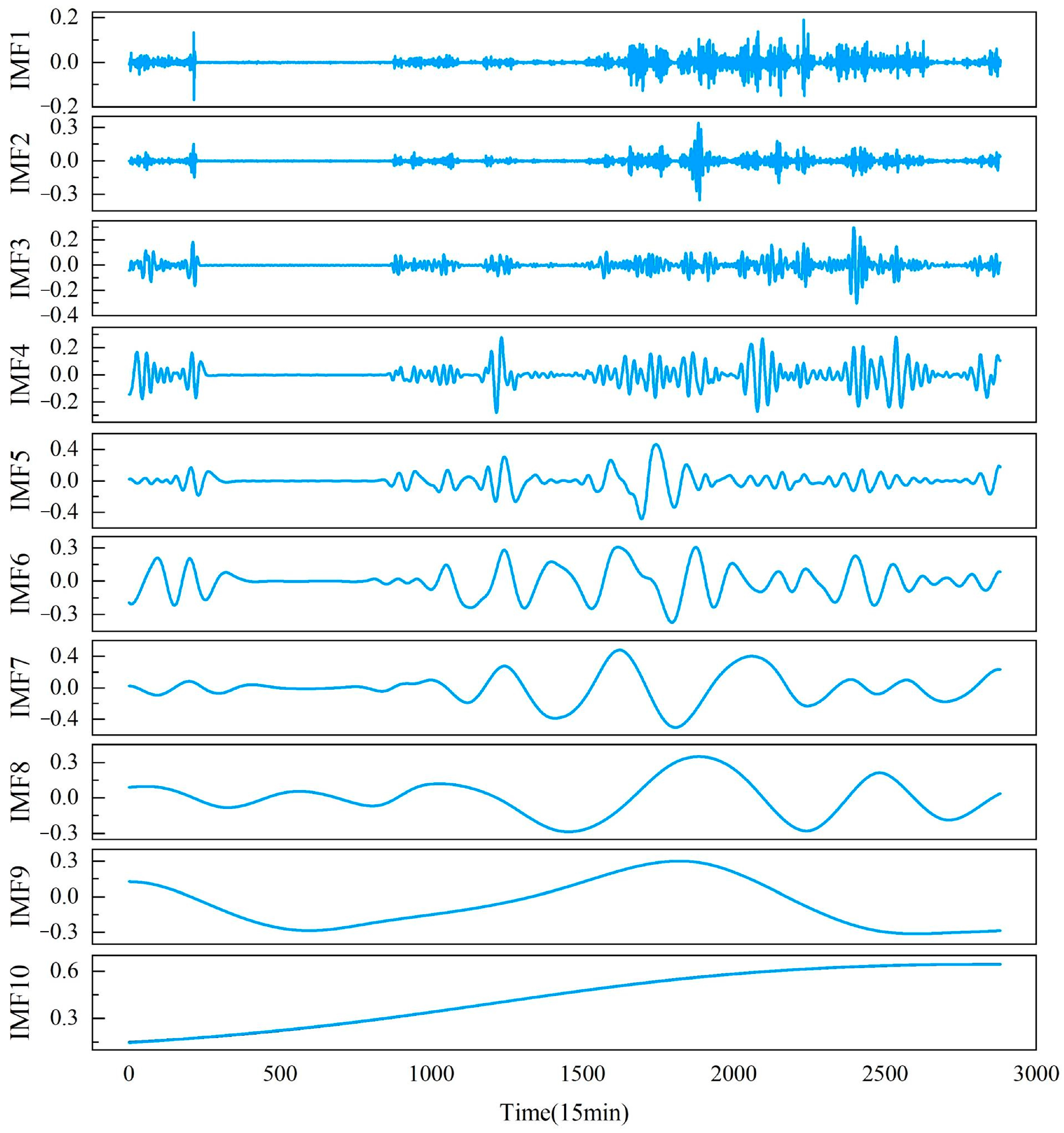
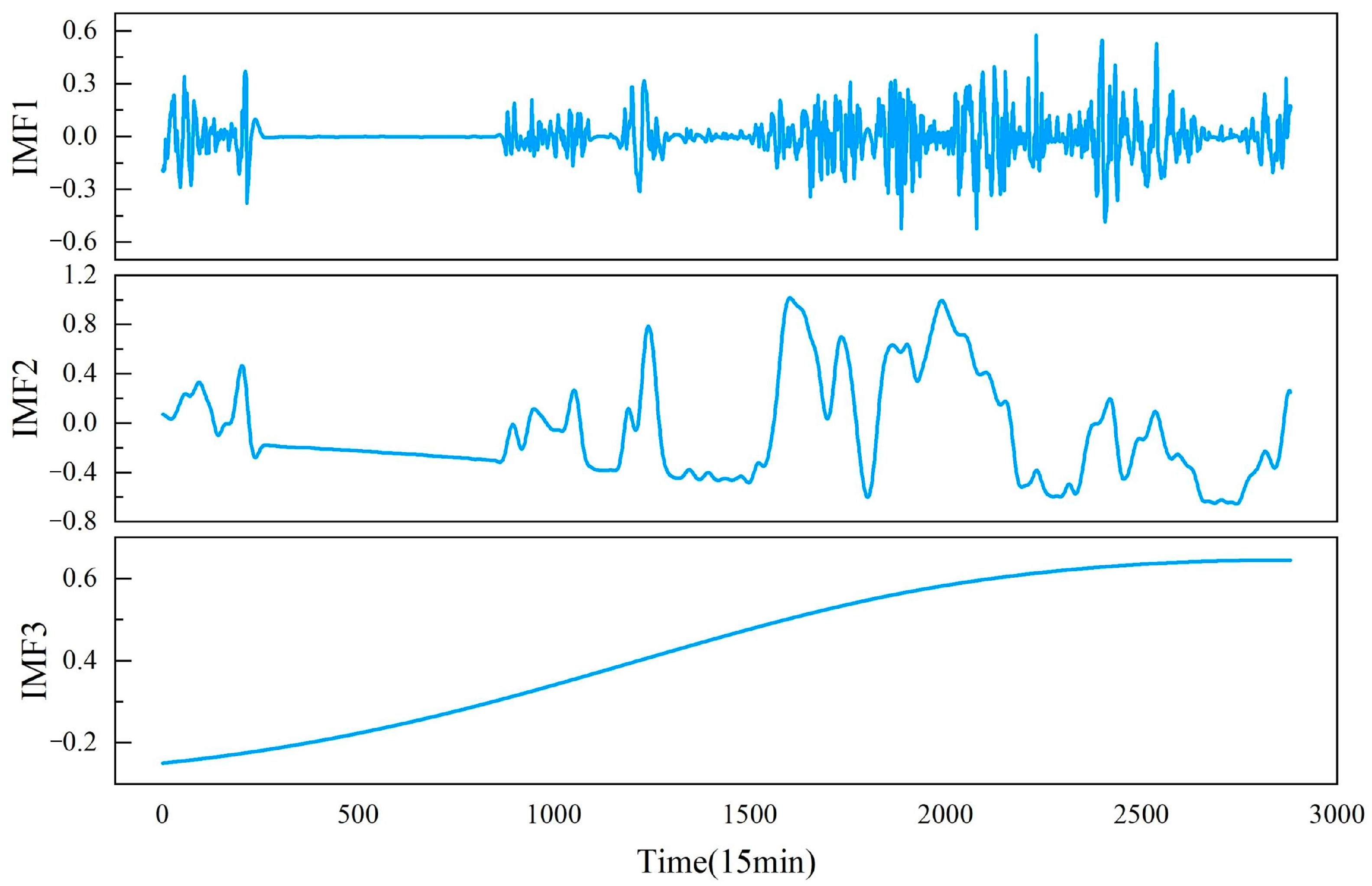
2.1. Intrinsic Combined Ensemble Empirical Mode Decomposition with Adaptive Noise

Empirical Mode Decomposition (EMD), proposed by Huang et al. in 1998, is a signal processing method suitable for nonlinear and non-stationary processes.

To overcome the limitations of EMD, Colominas et al. further improved CEEMDAN by introducing the Iterative Complete Ensemble Empirical Mode Decomposition with Adaptive Noise (ICEEMDAN) method. The core of this signal decomposition method lies in selecting the Kth IMF component of the white noise decomposed by EMD as the auxiliary noise. Through multiple iterations of noise addition and decomposition, ICEEMDAN comprehensively addresses the randomness and non-stationarity of data, thereby enhancing the stability and reliability of the final decomposition results and reducing the residual noise generated during reconstruction. The computational process is as follows:

• Based on the original wind power signal s, construct a new sequence $s^i$ by adding i groups of white noise ${\omega }^i$ to s, resulting in the first group of residues $R_1$.

  $$s^i=s+{\alpha }_0{E}_1({\omega }^i), R_1=〈M(s^i)〉$$

  (1)
  In Equation (1), $E_k(\cdot )$ represents the k-th mode component generated by EMD decomposition, $M(\cdot )$ represents the local mean of the signal generated by the EMD algorithm, and $〈\cdot 〉$ represents the overall mean.
• Calculate the first mode component $I_{\mathrm{IMF}1}=s-R_1$ iteratively to obtain the k-th group of residues $R_k$ and mode component $I_{\mathrm{IMFk}}$.

  $$R_k=〈M(R_{k-1}+{\alpha }_{k-1}{E}_k({\omega }^i))〉$$

  (2)

  $$I_{\mathrm{IMFk}}=R_{k-1}-R_k$$

  (3)
  In Equation (2), ${\alpha }_k$ can be expressed as ${\alpha }_k=\left\{\begin{array}{l}{\epsilon }_0\mathrm{std}(\lambda )/\mathrm{std}(E_1({\omega }^i)),\lambda =s\\ {\epsilon }_0\mathrm{std}(\lambda ),\lambda =R_k,k=1,2,\cdots ,K\end{array}\right.$.
• Repeat step 2 until the calculation is complete to obtain all wind power sequence mode components and the final residue.

2.2. Permutation Entroy

The PE (permutation entropy) algorithm, introduced by Bandt et al., is a method for characterizing the complexity of time series. Its core principle lies in assessing the irregularity in a time series through the examination of permutation patterns within its subsequences. A higher entropy value signifies greater complexity within the time series, whereas a lower value indicates a higher degree of regularity. Applied to the model proposed in this paper, the algorithmic formula is as follows:

• Consider a wind power generation sequence $X=\left\{x(i),i=1,2,\cdots ,k\right\}$, where i represent the number one of the wind power sequence.
• Perform phase space reconstruction on the time series, resulting in a reconstruction matrix Z with a given dimension m and time delay $\tau$.

  $$Z^T=\left[z(1) z(2) \cdot \cdot \cdot Z(k-(m-1)\tau )\right]$$

  (4)
  In Equation (4), $z(j)=\left\{x(j),x(j+\tau ),\cdots ,x(j+(m-1)\tau )\right\}$.
• Sort the elements of $z(j)$ in ascending order and record the sequence of elements in each row of the reconstruction matrix. Calculate the probability of occurrence for each element sequence to obtain $p_1,p_2,\cdots p_q$.
• Define the permutation entropy of wind power sequence X as:

  $$H\left(m\right)=-{\displaystyle {\sum }_{k=1}^q{P}_k\ln P_k}$$

  (5)
  In Equation (5), $P_k$ represents the probability of each element size relationship permutation in the reconstruction matrix Z, m is the given dimension, k is the number of subsequences, and q is the total number of elements.

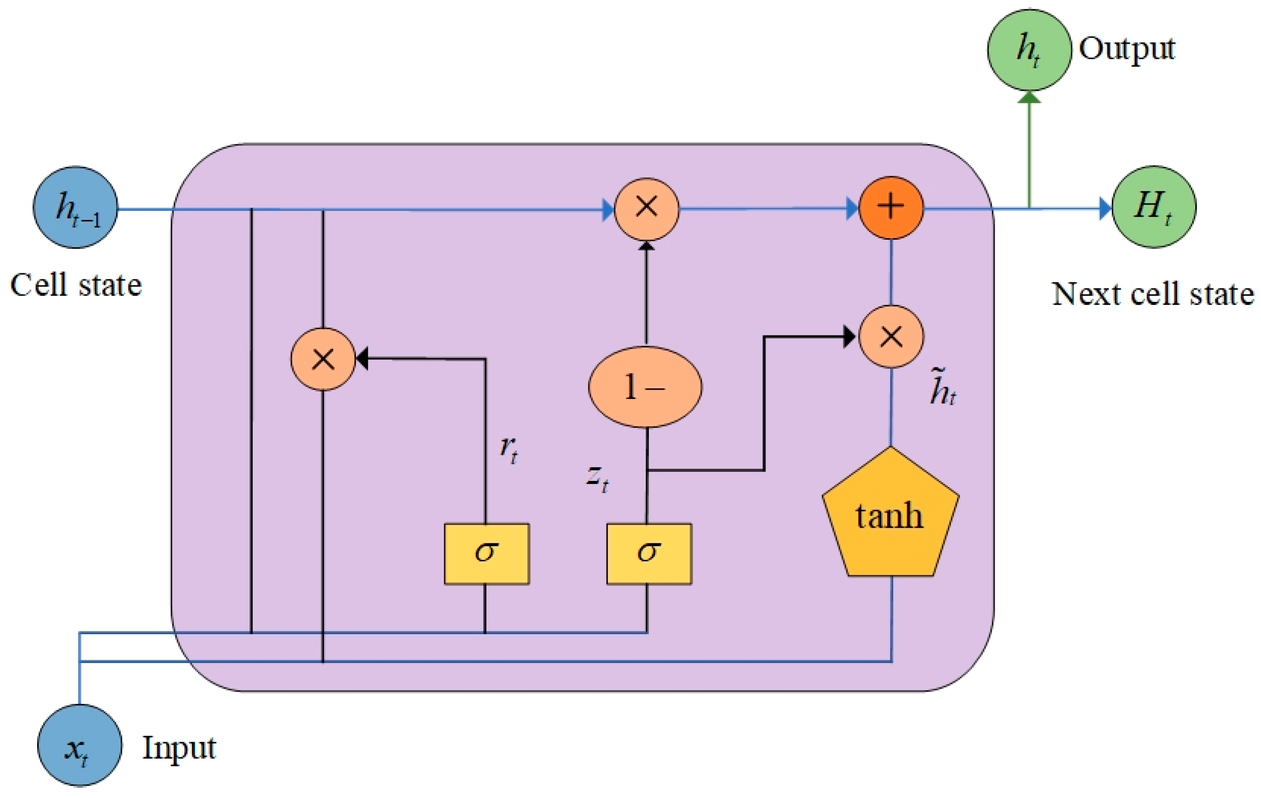
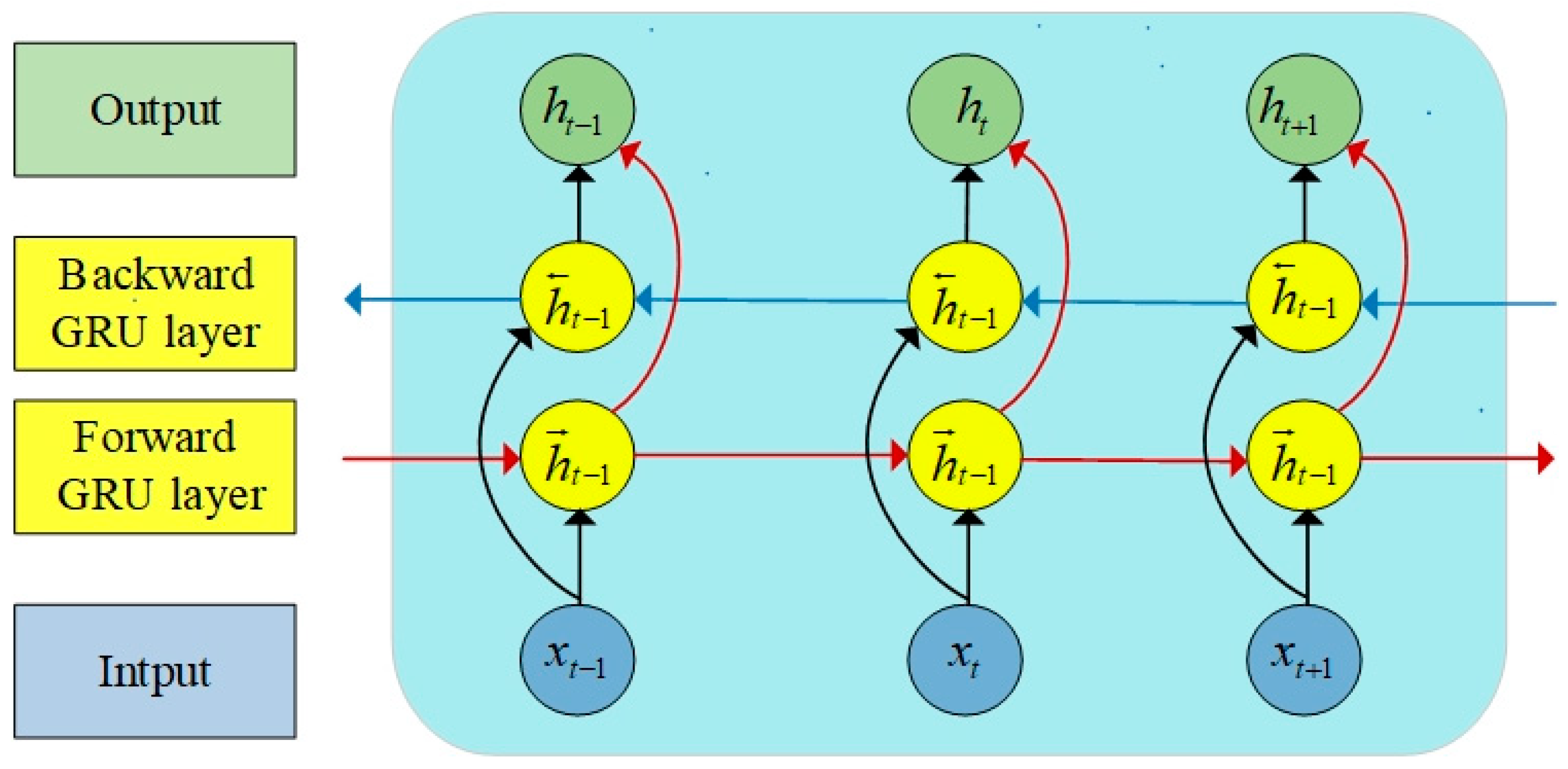
2.3. Bidirectional Gated Recurrent Unit

GRU (Gated Recurrent Unit) is an enhanced version of the Long Short-Term Memory (LSTM) network within the domain of recurrent neural networks. It is tailored to capture long-term dependencies within sequential data while boasting fewer parameters than LSTM, thereby mitigating computational costs. The core principle involves amalgamating the forget gate and input gate into a unified update gate. Through the management of information flow and state updates, it effectively reduces the parameter count and computational overhead. The model’s architectural depiction is presented in Figure 1, and the computational formulas are as follows:

$$z_t=\sigma \left({\mathit{W}}_z\cdot \left[{\mathit{h}}_{t-1},x_t\right]\right)$$

(6)

$$r_t=\sigma \left({\mathit{W}}_r\cdot \left[{\mathit{h}}_{t-1},x_t\right]\right)$$

(7)

$${\widehat{\mathit{h}}}_t=\tanh \left(\mathit{W}\cdot \left[r_t\odot {\mathit{h}}_{t-1},x_t\right]\right)$$

(8)

$${\mathit{h}}_t=\left(1-z_t\right)\odot {\eta }_{t-1}+z_k\odot {\widehat{\mathit{h}}}_t$$

(9)

In Equations (6)–(9), $z_t$ represents the update gate and $r_t$, $x_t$, ${\mathit{h}}_t$, and ${\widehat{\mathit{h}}}_t$ represent the reset gate, current time step input information, new cell vector, and hidden state vector, respectively. ${\mathit{W}}_z$, ${\mathit{W}}_r$, and W represent the weight matrices.

Because of the strong temporal characteristics inherent in wind power load data, information corresponding to both the previous time step (t − 1) and the current time step (t + 1) significantly impact the prediction results at time t during model training. Consequently, the GRU model fails to fully exploit the inherent information within wind power sequences. In contrast, the Bidirectional Recurrent Neural Network (BiGRU) model addresses this limitation by utilizing both past and future data to enhance prediction accuracy. This effectively overcomes the drawback of low data information utilization observed in the GRU network. Comprising two GRU models, BiGRU possesses the capability to capture bidirectional dependencies within sequential data, thereby enabling it to adapt to more complex sequence patterns. The network structure is visually depicted in Figure 2.

2.4. Multi-Head Attention

The attention mechanism (AM) is a computational method for the efficient allocation of information resources, prioritizing more crucial tasks to effectively mitigate information overload. In AM, input information is represented by key vectors (keys) and value vectors (values), while target information is represented by query vectors (queries). The weights of the value vectors are determined based on the similarity between the query vector and the key vector.

Following this, the final attention values are computed by aggregating the weighted value vectors. The fundamental formula is as follows:

$$S_{att}=W\times V$$

(10)

$$W=func\left(Q,K\right)$$

(11)

In Equations (10) and (11), $S_{att}$ is the attention value, Q represents the query vector, K represents the key vector in the key–value pairs, V represents the value vector in the key–value pairs, W represents the weight corresponding to V, and $func\left(\cdot \right)$ is the weight transformation function.

The multi-head attention mechanism originates from the Transformer [20] model. Its core principle involves mapping query, key, and value vectors to multiple spaces through distinct linear transformations, followed by calculating the scaled dot-product attention. The computational formula is as follows:

$$\mathrm{Attention}\left(Q,K,V\right)=softmax\left(\frac{Q{K}^T}{\sqrt{d_k}}\right)\cdot V$$

(12)

In Equation (12), $d_k$ represents the dimensionality of the keys, which is used to scale the dot product to prevent the issue of gradient vanishing.

Subsequently, vectors Q, K, and V of dimensionality d are transformed into single vectors of dimensionality $d/n$ using different weight matrices $W_i^Q$, $K_i$, and $Q_i$. Here, n denotes the number of parallel layers or heads, and these individual vectors are input into corresponding parallel attention layers. Finally, the outputs of each layer are concatenated and fused together using a linear layer to amalgamate all head output results.

As depicted in the multi-head attention section in Figure 3, in our model, we harness the powerful capability of the multi-head attention mechanism to capture diverse temporal scale features in time series, thereby predicting wind power sequences. The mathematical computation formula is as follows:

$$\mathrm{MHA}\left(Q,K,V\right)=\mathrm{Concat}\left({\mathrm{head}}_1,{\mathrm{head}}_2,\cdots ,{\mathrm{head}}_n\right)W^O$$

(13)

$$\begin{array}{l}{Q}_i=Q{W}_i^Q\\ K_i=K{W}_i^K\hspace{1em}\hspace{1em}\hspace{1em}i=1,2,\cdots ,n\\ V_i=V{W}_i^V\end{array}$$

(14)

In Equations (13) and (14), $W_i^Q\in {ℝ}^{d\times d_k}$, $W_i^K\in {ℝ}^{d\times d_k}$, $W_i^V\in {ℝ}^{d\times d_v}$, $W^O\in {ℝ}^{n{d}_v\times d}$, and $d_k=d_v=d/n$.

The multi-head attention architecture facilitates leveraging the complexity in input sequences and capturing long-range dependencies, thereby enhancing prediction accuracy. In this study, to mitigate overfitting, the model training employs Mean Squared Error (MSE) as the loss function and utilizes the Adam optimizer for parameter updates.

2.5. MHA-Bidirectional Gated Recurrent Unit

Although BiGRU performs effectively in handling wind power sequences, it lacks the ability to parallelize data processing, resulting in information overload and reduced computational efficiency when dealing with large datasets. To address this limitation, this study combines BiGRU with the multi-head attention mechanism (MHA), as depicted in Figure 3. This integrated model architecture effectively resolves the aforementioned issue. The core process involves utilizing the data trained through the BiGRU hidden layers as input for the MHA network. The decomposed Q, K, and V obtained are then fed into each head for attention value computation. Subsequently, the different results outputted from each channel are feature-weighted and concatenated through a connection layer to form the sequence.

2.6. DBO-MHA-Bidirectional Gated Recurrent Unit

The Dung Beetle Optimizer (DBO) optimization algorithm, introduces a novel swarm intelligence optimization approach. Its primary principle involves simulating five distinct behaviors observed in dung beetles, including rolling, dancing, foraging, stealing, and reproducing, to address optimization problems. Leveraging the DBO algorithm, the MHA-BiGRU model undergoes optimization of parameters such as the learning rate, the number of BiGRU neurons, the number of attention heads, the filter count, and regularization parameters. This optimization ensures the model’s convergence, with the objective of minimizing the loss function. The optimization formula is as follows:

$$f=\min (train\_loss(e\_s, h\_s, n\_l, l\_r, epoch))$$

(15)

In Equation (15), $e\_s$, $h\_s$, $n\_l$, $l\_r$, and epoch represent the number of attention heads, the filter count, the MHA-BiGRU model layers, the learning rate, and the regularization parameter, respectively. train_loss denotes the loss function during the training process.

2.7. Least Squares Support Vector Regression

Least Squares Support Vector Regression (LSSVR), proposed by Vapnik in the early 1990s, is a statistical learning method known for its fast training speed, good generalization performance, and strong ability to fit nonlinear functions.

It particularly excels in handling high-frequency signals, as its core algorithm transforms the solution of a convex quadratic optimization problem into solving a system of linear equations. Consequently, LSSVR requires fewer parameters to train compared with SVR, resulting in faster training speed.

Suppose there is a training set ${\left\{\left({\mathit{x}}_i,y_i\right)\right\}}_{i=1}^n$, where ${\mathit{x}}_i\in {\mathit{R}}^d$ represents the input and $y_i\in \mathit{R}$ represents the output. The model calculation formula is as follows:

$$f(\mathit{x})={\mathit{w}}^T\mathit{\varphi }(\mathit{x})+b={\displaystyle \sum _{i=1}^n{\alpha }_i\kappa ({\mathit{x}}_i,\mathit{x})+b}$$

(16)

In Equation (16), $\mathit{w}={\displaystyle \sum _{i=1}^n{\alpha }_i\mathit{\varphi }({\mathit{x}}_i)}$, $\mathit{w}$ represents the weight vector, $\mathit{\varphi }(\cdot )$ denotes the non-linear mapping from the input space to the high-dimensional feature space, ${\alpha }_i$ stands for the Lagrange multiplier, $\kappa ({\mathit{x}}_i,\mathit{x})$ is the kernel function, and b is the bias term.

2.8. Regularized Extreme Learning Machine

Extreme Learning Machine (ELM) [28] is a machine learning algorithm proposed by Professor Huang from Nanyang Technological University in 2004. Its distinguishing feature is a single hidden layer feedback neural network. It can be transformed into solving the generalized inverse problem of the M-P matrix by simply adding a least squares minimum norm problem. Consequently, ELM has fewer model parameters and boasts a fast training speed. It demonstrates excellent capability in handling medium-frequency sequence information.

Consider a wind power sequence set $({\mathit{X}}_i,{\mathit{t}}_i)$, where the model input is denoted by ${\mathit{X}}_i={[x_{i1},x_{i2},\cdots ,x_{in}]}^T$ and the model output by ${\mathit{t}}_i={[t_{i1},t_{i2},\cdots ,t_{in}]}^T$. Then, an ELM network with L hidden layer nodes can be defined as:

$${\displaystyle \sum _{i=1}^L{\beta }_i\times g({\omega }_i\cdot x_j+b_i)}=o_j , j=1,2,\cdots ,N$$

(17)

In Equation (17), $g(\cdot )$ represents the activation function, ${\omega }_i$ denotes the connection weights between the output layer and the hidden layer, ${\beta }_i$ signifies the output weights between the hidden layer and the output layer, $b_i$ stands for the bias of the i-th hidden unit, and $o_j$ represents the network output. The calculation formula used to minimize the output error is as follows: $\underset{\beta }{\min }{‖\mathit{H}\beta -\mathit{T}‖}_F$, where H denotes the hidden layer output and T represents the expected output.

To improve the model’s generalization performance, a regularization parameter $\lambda$ is introduced to solve $\beta$, effectively addressing numerical instability issues when computing the pseudo-inverse of H. The computation process of the RELM model, utilizing a regularized least squares method to solve $\beta$, is mathematically expressed as follows: $\underset{\beta }{\min }{‖\mathit{H}\beta -\mathit{T}‖}_F+(1/\lambda )\cdot {‖\beta ‖}_F$.

2.9. Composition of the Proposed Model

Drawing from the aforementioned methodologies, this study introduces a multiscale hybrid wind power prediction model that integrates ICEEMDAN signal decomposition, permutation entropy (PE) reconstruction, and LSSVR-RELM-MHA-BiGRU. The model parameters are optimized using the DBO optimization algorithm. The overall model workflow, as depicted in Figure 4, is further elucidated with detailed step-by-step explanations as follows:

Step 1: ICEEMDAN decomposes the original wind power data into multiple Intrinsic Mode Function (IMF) components and a residual R. Using permutation entropy (PE), all IMF components are reconstructed to reduce computational complexity. Subsequently, the reconstructed components are categorized into high-frequency, medium-frequency, and low-frequency components based on their PE values.

Step 2: The DBO optimization algorithm is applied to optimize the hyperparameters of the MHA-BiGRU model. The optimized model is then used to predict the IMF low-frequency component after reconstruction.

Step 3: The high-frequency, medium-frequency, and low-frequency components are separately fed into the LSSVR, RELM, and MHA-BiGRU models, respectively. Predictions are obtained for each component.

Step 4: The predictions for the high-, medium-, and low-frequency IMF components are aggregated to obtain the final prediction result.

3. Research Study

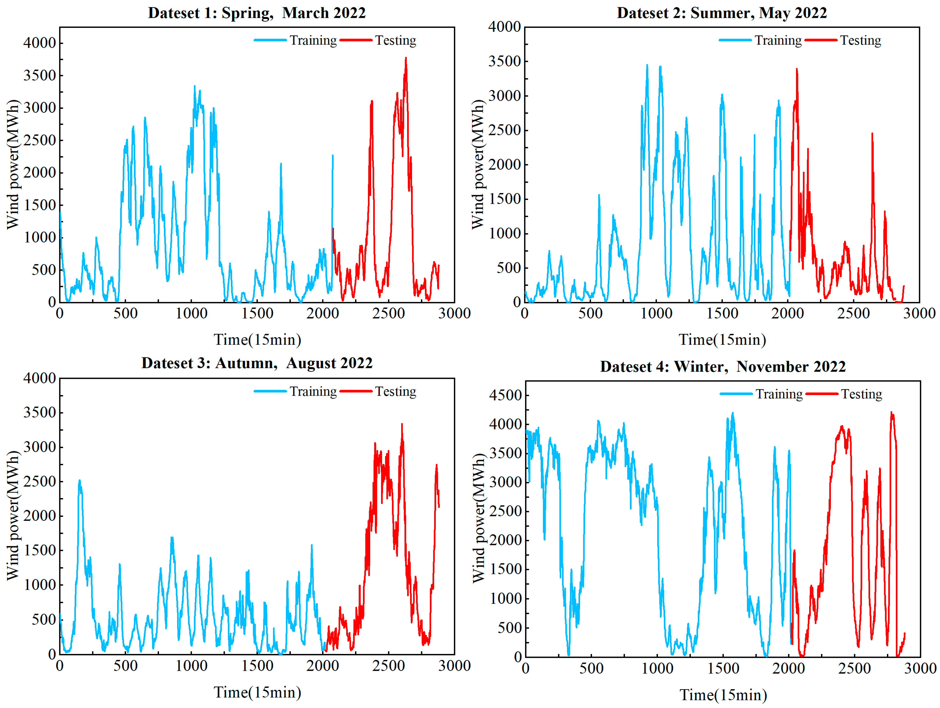
3.1. Data Description

The wind power dataset in this paper is sourced from a wind farm operated by Elia in Belgium. To validate the accuracy of the model, four sets of power data from different seasons were selected as the original data for the model. The wind power data were recorded every 15 min. Details of the data are provided in Figure 5 and

Table 1. Basic information of the four monthly wind power datasets.

Months	Dataset	Data Length	Max	Min	Mean	Std Dev
March	All (MWh)	2880	3780.86	1.43	920.67	911.52
	Training (MWh)	2016	3780.86	16.51	1146.53	976.85
	Testing (MWh)	864	2271.29	1.43	393.69	382.49
May	All (MWh)	2880	3483.90	0.21	862.15	918.57
	Training (MWh)	2016	3455.84	0.21	784.92	869.87
	Testing (MWh)	864	3483.90	2.18	1042.35	1000.30
August	All (MWh)	2880	2751.17	2.53	580.44	482.30
	Training (MWh)	2016	2523.70	2.53	543.60	457.46
	Testing (MWh)	864	2751.17	7.70	666.39	525.85
November	All (MWh)	2880	4206.60	6.31	2082.61	1361.31
	Training (MWh)	2016	4206.60	18.08	2229.31	1345.26
	Testing (MWh)	864	3810.65	6.31	1740.32	1336.83

. During the data collection process, issues such as missing data and data errors are inevitable, which can significantly affect the accuracy of model predictions. Therefore, this paper adopts the method of removing zeros and mean interpolation to preprocess the data. Each month contains 2880 data points, and each set of data is divided into training and testing sets at a ratio of 7:3.

In Table 1 and Figure 5, it is visually evident that the wind power data exhibit significant randomness and non-stationarity. Because of the large numerical values in the wind power dataset, all data are normalized through scaling to facilitate observing the data characteristics.

Subsequently, the ICEEMDAN method is employed to decompose the wind power sequence into signals (as shown in Figure 6). During decomposition, 50 instances of white noise are added, with a standard deviation (Ntsd) set to 0.2 and a maximum allowable iteration of 100. ICEEMDAN decomposes the original sequence into multiple Intrinsic Mode Function (IMF) sub-sequences. Taking the wind power sequence of March as an example, the decomposition results are illustrated in Figure 6.

As shown in Figure 6, the data are decomposed into multiple IMF components. According to the workflow diagram, in this paper, it is necessary to predict each reconstructed sub-component and then aggregate the prediction results to obtain the final forecast. However, during this process, the computational complexity significantly increases, leading to substantial errors in the prediction results. Therefore, the permutation entropy (PE) method is employed to calculate the entropy value of each sub-component separately, re-quantifying the complexity of each sub-component.

Simultaneously, all sub-components are reconstructed into three new sub-components, including high-frequency, medium-frequency, and low-frequency sub-components, thus reducing the sequence complexity. The PE values of each sub-component are shown in

Table 2. Permutation entropy of each sample.

Component	PE
IMF 1	0.9936
IMF 2	0.8908
IMF 3	0.7174
IMF 4	0.5798
IMF 5	0.4913
IMF 6	0.4424
IMF 7	0.4135
IMF 8	0.3999
IMF 9	0.3911
IMF 10	0.0451

.

Based on the entropy values, IMF1–IMF3 are selected as high-frequency components, IMF4–IMF9 as medium-frequency components, and IMF10 as the low-frequency component. The newly reconstructed sub-components are illustrated in Figure 7.

3.2. Performance Metrics

To better assess the performance of the model predictions, this study employs three different error evaluation metrics including Root Mean Squared Error (RMSE), Mean Absolute Error (MAE), and Mean Absolute Percentage Error (MAPE). Mean Absolute Percentage Error (MAPE) is used to measure forecast accuracy; Mean Absolute Error (MAE) reflects the actual situation of errors; and the RMSE value reflects the sensitivity to the abnormal value of the wind power sequence.

$$e_{\mathrm{RMSE}}=\sqrt{\frac{{\displaystyle \sum _{i=1}^n{\left|f\left(x_i\right)-a\left(x_i\right)\right|}^2}}{n}}$$

(18)

$$e_{\mathrm{MAE}}=\frac{1}{n}{\displaystyle \sum _{i=1}^n\left|f\left(x_i\right)-a\left(x_i\right)\right|}$$

(19)

$$e_{\mathrm{MAPE}}=\frac{1}{n}{\displaystyle \sum _{i=1}^n\left|\frac{f\left(x_i\right)-a\left(x_i\right)}{a\left(x\right)}\right|\times 100\%}$$

(20)

The above equation represents the calculation of the Mean Absolute Percentage Error (MAPE) metric, where $a\left(x_i\right)$ denotes the actual observed value of the i-th training sample, $f\left(x_i\right)$ represents the predicted value of the i-th sample, and n represents the total number of samples.

4. Comparative Results

Experiment and Results Analysis

This study employed nine models to forecast wind power sequences for four different seasonal months, as outlined in

Table 3. Code name for each model.

Name	Model
Model 1	LSSVR
Model 2	RELM
Model 3	BiGRU
Model 4	MHA-BiGRU
Model 5	ICEEMDAN-LSSVR
Model 6	ICEEMDAN-RELM
Model 7	ICEEMDAN-MHA-BiGRU
Model 8	ICEEMDAN-LSSVR-RELM-MHA-BiGRU
Proposed	ICEEMDAN-LSSVR-RELM-DBO-MHA-BiGRU

. A comparative analysis was conducted between the proposed ICEEMDAN-LSSVR-RELM-DBO-MHA-BiGRU model and other models including LSSVR, RELM, BiGRU, MHA-BiGRU, ICEEMDAN-LSSVR, ICEEMDAN-RELM, ICEEMDAN-MHA-BiGRU, and ICEEMDAN-LSSVR-RELM-MHA-BiGRU. The evaluation was performed using three different metrics including MAE, RMSE, and MAPE. The results were visually presented using bar charts, radar charts, and stacked bar charts, as depicted in Figure 8 and summarized in

Table 4. Statistical measures of wind power prediction.

Dataset	Models	RMSE	MAE	MAPE
March	Model 1	0.7563	0.8021	1.4089
	Model 2	0.5039	0.6671	0.8476
	Model 3	0.4657	0.4332	0.6599
	Model 4	0.3605	0.3624	1.3988
	Model 5	0.4105	0.3766	0.6821
	Model 6	0.4710	0.5691	1.2042
	Model 7	0.3933	0.2968	0.6470
	Model 8	0.2053	0.2012	0.3535
	Proposed	0.1757	0.1133	0.2297
May	Model 1	0.6852	0.5711	1.4820
	Model 2	0.5743	0.6113	0.7851
	Model 3	0.5670	0.5053	0.5627
	Model 4	0.3798	0.4182	0.8501
	Model 5	0.3983	0.3398	1.2908
	Model 6	0.3422	0.2243	0.3348
	Model 7	0.2862	0.2331	1.2788
	Model 8	0.1528	0.1662	0.2924
	Proposed	0.1354	0.1178	0.2102
August	Model 1	0.6203	0.7706	1.675
	Model 2	0.5104	0.5963	1.6358
	Model 3	0.4915	0.4784	0.85306
	Model 4	0.4688	0.3796	1.1223
	Model 5	0.4617	0.3554	0.5117
	Model 6	0.3813	0.3048	0.4701
	Model 7	0.3557	0.3291	0.7367
	Model 8	0.2285	0.2093	0.3467
	Proposed	0.1661	0.1243	0.1069
November	Model 1	0.7021	0.6053	1.2463
	Model 2	0.6120	0.5825	1.2038
	Model 3	0.5811	0.5351	0.9602
	Model 4	0.4655	0.4528	1.1745
	Model 5	0.3842	0.3413	0.8221
	Model 6	0.3522	0.3227	1.1934
	Model 7	0.3106	0.3067	0.6332
	Model 8	0.1903	0.2026	0.3374
	Proposed	0.1416	0.1086	0.2397

, providing a comprehensive comparison of the predictive performance of the models.

Upon careful examination of Table 4 and Figure 8, the following conclusions can be drawn:

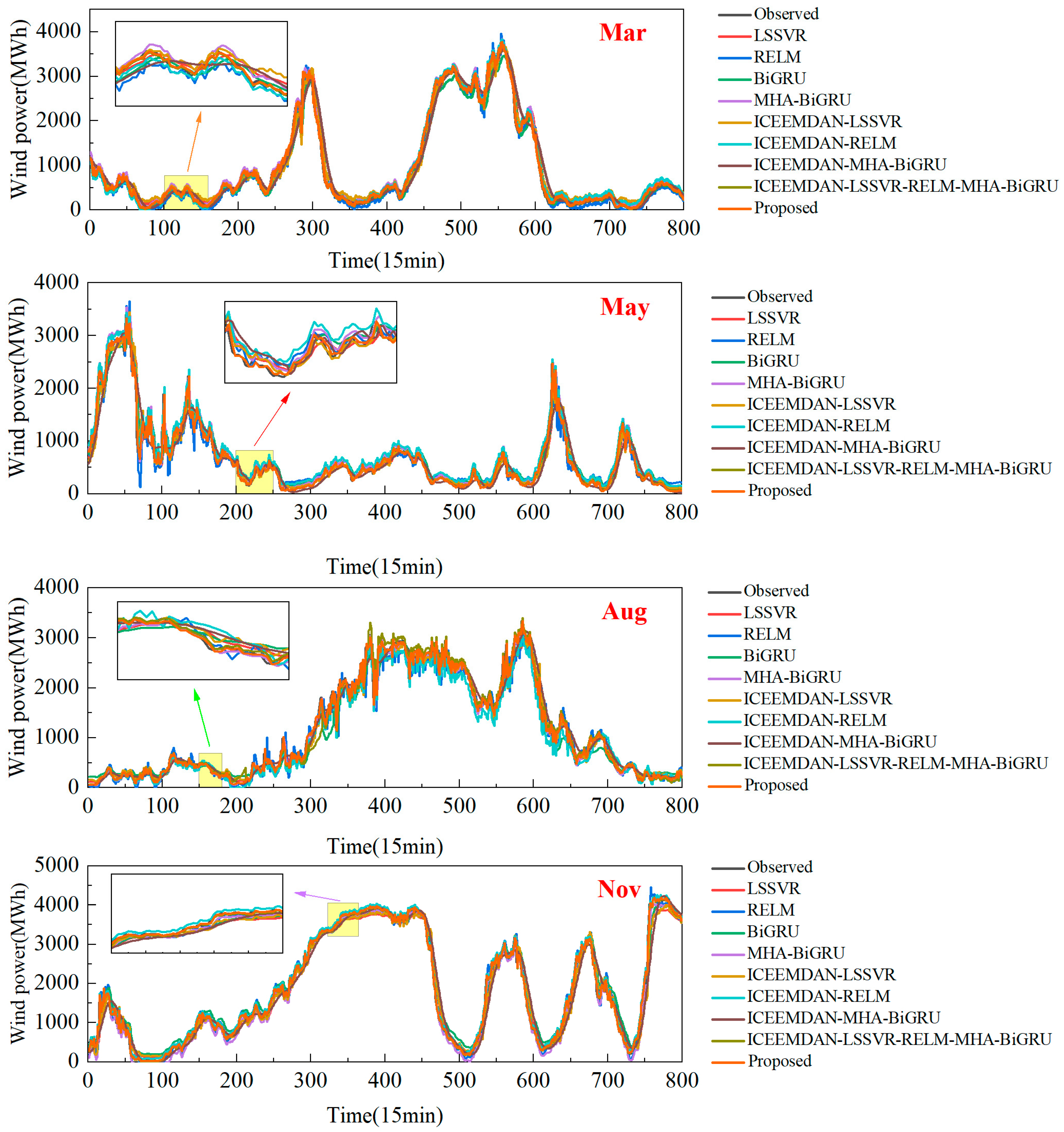
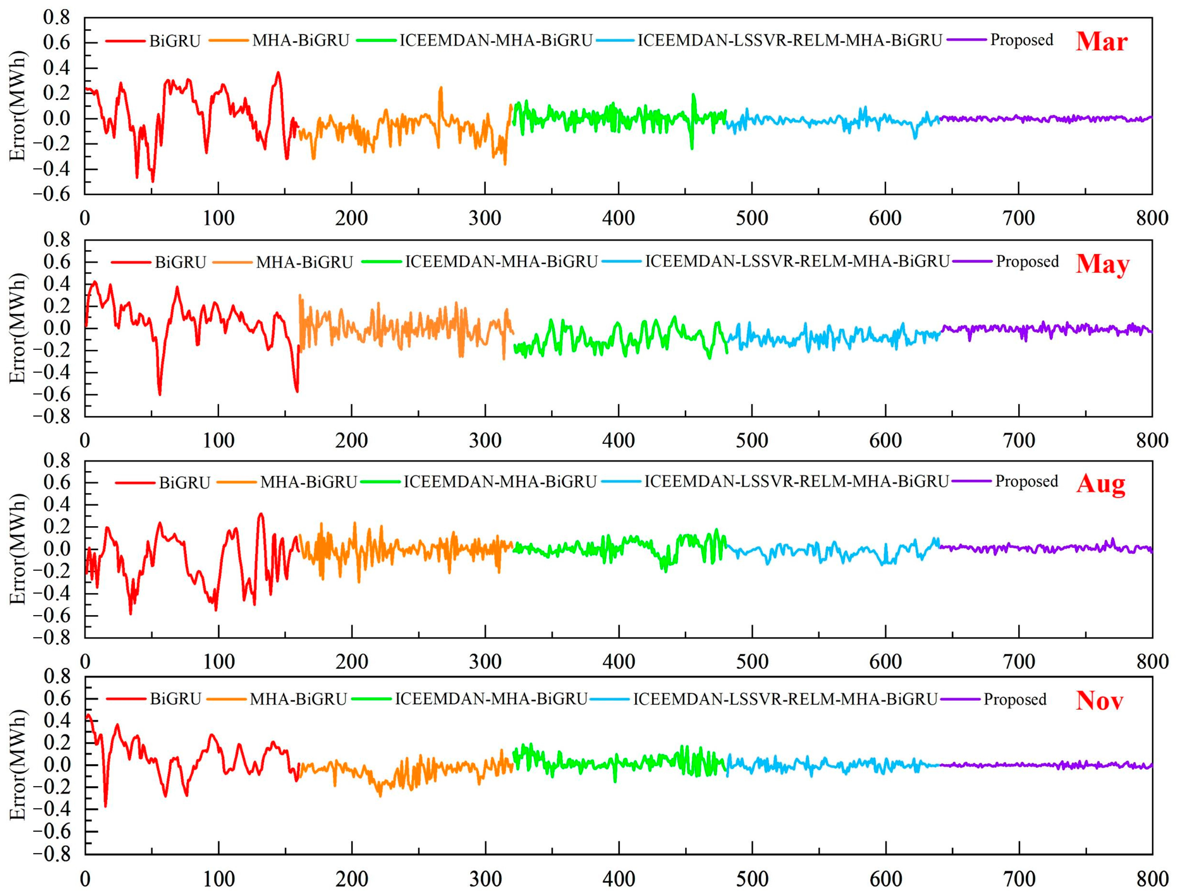
• The comparison of the LSSVR, RELM, and BiGRU models suggests that multiscale hybrid models outperform single-scale models in wind power sequence prediction.
• The evaluation of the BiGRU and MHA-BiGRU models reveals a notable decrease of 18.72% in RMSE and 7.08% in MAE for the May forecast. Additionally, for the March forecasts, the RMSE values decrease by approximately 10%, indicating that the incorporation of multi-head attention mechanisms enhances predictive accuracy.
• The inclusion of decomposition algorithms generally enhances predictive performance in wind power prediction compared with single models. For example, in the August metrics, the LSSVR, RELM, and BiGRU models incorporating the ICEEMDAN decomposition algorithm exhibit reductions of 25.57%, 25.29%, and 27.63% in RMSE values, respectively, along with approximately 20% decreases in the other metrics. This underscores the effectiveness of models incorporating decomposition algorithms in improving prediction accuracy.
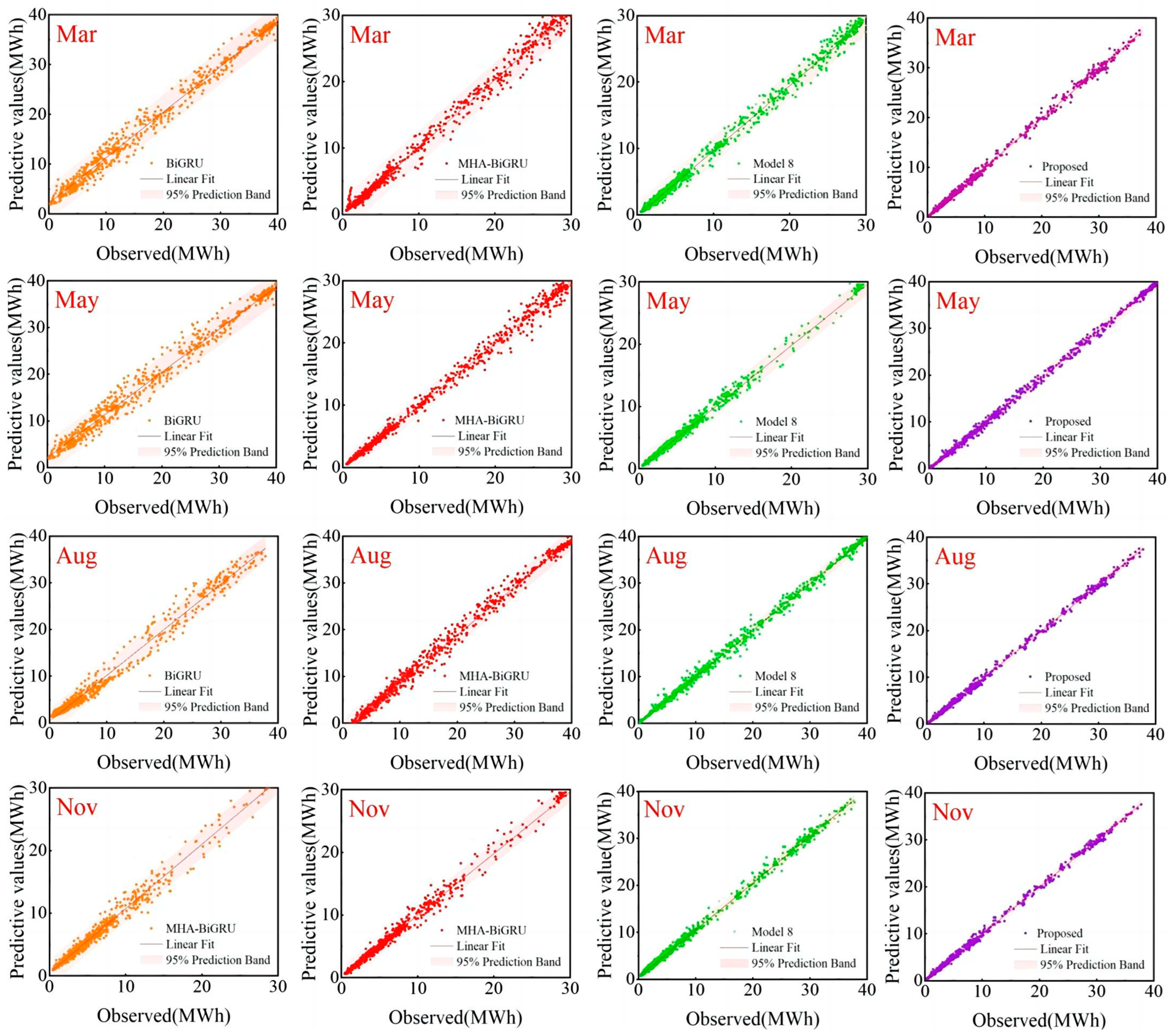
• The comparison between Model 8 and the single-scale models combined with decomposition algorithms indicates that hybrid algorithms generally exhibit superior predictive performance. For instance, in the radar chart of MAPE values in Figure 7, the proposed model consistently exhibits the lowest values along its axes. Furthermore, in terms of RMSE values for March, Model 8 demonstrates a 57.20% reduction compared with Model 5. This underscores the advantage of multiscale hybrid algorithms in achieving smaller errors and higher predictive accuracy.
• The evaluation of Model 8 against the proposed model highlights improvements in predictive performance with the introduction of DBO optimization algorithms. For instance, in the November forecast, there are reductions of 25.59%, 46.40%, and 28.96% in the RMSE, MAE, and MAPE values, respectively. This indicates that the incorporation of DBO optimization algorithms enhances predictive performance, rendering the model proposed in this study more suitable for wind power sequence prediction.

As shown in Figure 6, the data are decomposed into multiple IMF components. According to the workflow diagram, in this paper, it is necessary to predict each reconstructed sub-component and then aggregate the prediction results to obtain the final forecast. However, during this process, the computational complexity significantly increases, leading to substantial errors in the prediction results. Therefore, the permutation entropy (PE) method is employed to calculate the entropy value of each sub-component separately, re-quantifying the complexity in each sub-component.

Simultaneously, all sub-components are reconstructed into three new sub-components, including high-frequency, medium-frequency, and low-frequency sub-components, thus reducing the sequence complexity. The PE values of each sub-component are shown in Table 2. Based on the entropy values, IMF1–IMF3 are selected as high-frequency components, IMF4–IMF9 as medium-frequency components, and IMF10 as the low-frequency component. The newly reconstructed sub-components are illustrated in Figure 7.

To further validate the accuracy of the proposed model, Figure 9 illustrates a comparison of forecasts between the ICEEMDAN-LSSVR-RELM-DBO-MHA-BiGRU model and other models for four months. Figure 10 displays the relative error plots for the BiGRU, MHA-BiGRU, ICEEMDAN-MHA-BiGRU, and ICEEMDAN-LSSVR-RELM-MHA-BiGRU models and the proposed model. Figure 11 presents linear regression plots with 95% confidence intervals for the true values and predictions of these five models.

Upon closer examination of the magnified portions in Figure 9, it is evident that models incorporating decomposition algorithms and multiscale hybrid models exhibit the highest degree of fitting. This underscores the effectiveness of the proposed model. In Figure 10, it can be observed that the proposed method demonstrates the smallest fluctuation range in relative errors. Moreover, in Figure 11, the linear regression confidence band for the proposed model is the narrowest. Particularly, after incorporating attention mechanisms and decomposition algorithms, the scatter plots become more concentrated, and the confidence band notably narrows.

Based on the aforementioned analysis, it can be concluded that the LSSVR-RELM-MHA-BiGRU and data decomposition model proposed in this study exhibits effectiveness and applicability and yields satisfactory prediction results in wind power forecasting.

5. Discussion

This paper aims to improve the accuracy of wind power prediction. Based on the comparison of prediction errors among various models and the proposed model, as well as the verification of methods such as error bands and confidence intervals, it can be concluded that the proposed method indeed improves the accuracy of wind power prediction. These results are based solely on historical data prediction, similar to the methods used to handle historical data in the literature [19,20,21,22,23,24,25], but the accuracy in this paper may be relatively higher. This paper combines machine learning, deep learning, and signal processing methods, thus contributing a new method of artificial intelligence hybrid prediction of wind power. Building on the research of previous scholars, the method introduced in this paper, which incorporates a multi-head attention mechanism and data-denoising technology, may provide some reference for subsequent researchers.

The multiscale hybrid wind power prediction model proposed in this study advances the capability of single-step prediction in wind power forecasting, offering valuable insights for the rational planning of power systems. However, there are avenues for improving prediction methods, which include the following:

• This study relies solely on historical wind power data without considering additional factors such as geographical conditions and turbine statuses, which can significantly influence wind power prediction accuracy. Thus, future research could explore integrating multiple factors to enable multi-step prediction.
• The dataset used in this study is limited to a single wind farm, which may restrict the model’s ability to generalize across different environments. Future endeavors should aim to validate the proposed model using data from multiple wind farms to enhance its robustness and applicability.

6. Conclusions

This paper proposes a multiscale hybrid model incorporating a multi-head attention mechanism and data decomposition technique and optimizes the parameters of the low-frequency signal segment of the model using the beetle optimization algorithm. By introducing the data decomposition technique, the most crucial information of the wind power series is extracted, thus eliminating the redundancy in feature selection required by conventional algorithms. On this basis, a multi-head attention mechanism is introduced to extract features of the low-frequency signal close to the time step, further addressing the issue of information loss after data decomposition, thereby limiting the impact of random fluctuations in wind power. The feature correlation results calculated by the sample entropy method can be directly applied to input variables. It avoids the data clustering used in conventional methods. The beetle algorithm is employed to improve prediction accuracy, avoiding the influence of artificially determined network hyperparameters.

The simulation results on datasets demonstrate that the proposed method achieves higher prediction accuracy compared with previous algorithms. This approach provides a new avenue for researchers to improve the prediction accuracy of wind power series by introducing methods such as the multi-head attention mechanism.

However, only single-step prediction is considered, and future work can focus on improving the method for multi-step prediction. Additionally, since most neural networks contain hyperparameters, this approach is theoretically applicable to other neural networks and can be further validated in future studies.

References

1. Global Wind Energy Council. 2022 Global Wind Report; Global Wind Energy Council (GWEC): Brussels, Belgium, 2023; pp. 6–7. [Google Scholar]
2. Yuan, X.; Chen, C.; Yuan, Y.; Huang, Y.; Tan, Q. Short-term wind power prediction based on LSSVM–GSA model. Energy Convers. 2015, 101, 393–401. [Google Scholar] [CrossRef]
3. Hu, S.; Xiang, Y.; Zhang, H.; Xie, S.; Li, J.; Gu, C.; Sun, W.; Liu, J. Hybrid forecasting method for wind power integrating spatial correlation and corrected numerical weather prediction. Appl. Energy 2021, 293, 116951. [Google Scholar] [CrossRef]
4. Ye, L.; Dai, B.; Li, Z.; Pei, M.; Zhao, Y.; Lu, P. An ensemble method for short-term wind power prediction considering error correction strategy. Appl. Energy 2022, 322, 119475. [Google Scholar] [CrossRef]
5. Wang, J.; Hu, J.; Ma, K.; Zhang, Y. A self-adaptive hybrid approach for wind speed forecasting. Renew. Energy 2015, 78, 374–385. [Google Scholar] [CrossRef]
6. Xiong, B.; Meng, X.; Xiong, G.; Ma, H.; Lou, L.; Wang, Z. Multi-branch wind power prediction based on optimized variational mode decomposition. Energy 2022, 8, 11181–11191. [Google Scholar]
7. Costa, A.; Crespo, A.; Navarro, J.; Lizcano, G.; Madsen, H.; Feitosa, E. A review on the young history of the wind power short-term prediction. Renew. Sustain. Energy 2008, 12, 1725–1744. [Google Scholar] [CrossRef]
8. Wang, H.; Han, S.; Liu, Y.; Yan, J.; Li, L. Sequence transfer correction algorithm for numerical weather prediction wind speed and its application in a wind power forecasting system. Appl. Energy 2019, 237, 1–10. [Google Scholar] [CrossRef]
9. Liang, T.; Zhao, Q.; Lv, Q.; Sun, H. A novel wind speed prediction strategy based on Bi-LSTM, MOOFADA and transfer learning for centralized control centers. Energy 2021, 230, 120904. [Google Scholar] [CrossRef]
10. Erdem, E.; Shi, J. ARMA based approaches for forecasting the tuple of wind speed and direction. Energy 2011, 88, 1405–1414. [Google Scholar] [CrossRef]
11. Valipour, M.; Banihabib, M.; Behbahani, S. Comparison of the ARMA, ARIMA, and the autoregressive artificial neural network models in forecasting the monthly inflow of Dez dam reservoir. J. Hydrol 2013, 476, 433–441. [Google Scholar] [CrossRef]
12. Awad, M.; Khanna, R. Support vector regression. In Efficient Learning Machines; Springer: Berlin/Heidelberg, Germany, 2015; pp. 67–80. [Google Scholar]
13. Huang, G.-B.; Zhu, Q.-Y.; Siew, C.-K. Extreme learning machine: A new learning scheme of feedforward neural networks. In Proceedings of the Conference Extreme Learning Machine: A New Learning Scheme of Feedforward Neural Networks, Budapest, Hungary, 25–29 July 2004; Volume 2, pp. 985–990. [Google Scholar]
14. Li, C.; Tang, G.; Xue, X.; Saeed, A.; Hu, X. Short-term wind speed interval prediction based on ensemble GRU Model. IEEE Trans. Sustain. Energy 2020, 11, 1370–1380. [Google Scholar] [CrossRef]
15. Wang, X.; Wang, C.; Li, Q. Short-term wind power prediction using GA-ELM. Open Electr. Electron. Eng. J. 2017, 11, 48–56. [Google Scholar] [CrossRef]
16. Zhai, X.; Ma, L. Medium and long-term wind power prediction based on artificial fish swarm algorithm combined with extreme learning machine. Int. Core J. Eng. 2019, 5, 265–272. [Google Scholar]
17. Tan, L.; Han, J.; Zhang, H. Ultra-short-term wind power prediction by salp swarm algorithm-based optimizing extreme learning machine. IEEE Access 2020, 8, 44470–44484. [Google Scholar] [CrossRef]
18. Bouktif, S.; Fiaz, A.; Ouni, A.; Serhani, M.A. Multi-Sequence LSTM-RNN Deep Learning and Metaheuristics for Electric Load Forecasting. Energies 2020, 13, 391. [Google Scholar] [CrossRef]
19. Gundu, V.; Simon, S.P. PSO–LSTM for short term forecast of heterogeneous time series electricity price signals. J. Ambient. Intell. Hum. Comput. 2021, 12, 2375–2385. [Google Scholar] [CrossRef]
20. Meng, Y.; Chang, C.; Huo, J.; Zhang, Y.; Mohammed Al-Neshmi, H.M.; Xu, J.; Xie, T. Research on Ultra-Short-Term Prediction Model ofWind Power Based on Attention Mechanism and CNN-BiGRU Combined. Front. Energy Res. 2022, 10, 920835. [Google Scholar] [CrossRef]
21. Wang, Y.; Chen, J.; Chen, X.; Zeng, X.; Kong, Y.; Sun, S.; Guo, Y.; Liu, Y. Short-term load forecasting for industrial customers based on TCN-LightGBM. IEEE Trans. Power Syst. 2021, 36, 1984–1997. [Google Scholar] [CrossRef]
22. Chi, D.; Yang, C. Wind power prediction based on WT-BiGRU-attention-TCN model. Front. Energy Res. 2023, 11, 1156007. [Google Scholar] [CrossRef]
23. Zhang, Y.; Zhang, L.; Sun, D.; Jin, K.; Gu, Y. Short-Term Wind Power Forecasting Based on VMD and a Hybrid SSA-TCN-BiGRU Network. Appl. Sci. 2023, 13, 9888. [Google Scholar] [CrossRef]
24. Gao, X.; Li, X.; Zhao, B.; Ji, W.; Jing, X.; He, Y. Short-term Electricity Load Forecasting Model based on EMD-GRU with Feature Selection. Energies 2019, 12, 1140. [Google Scholar] [CrossRef]
25. Colominas, M.A.; Schlotthauer, G.; Torres, M.E.; Flandrin, P. Noise-assisted EMD methods in action. Adv. Adapt. Data Anal. 2012, 4, 1250025. [Google Scholar] [CrossRef]
26. Colominas, M.A.; Schlotthauer, G.; Torres, M.E. Improved complete ensemble EMD:A suitable tool for biomedical signal processing. Biomed. Signal Process. Control 2014, 14, 19–29. [Google Scholar] [CrossRef]
27. Xue, J.; Shen, B. Dung beetle optimizer: A new meta-heuristic algorithm for global optimization. J. Supercomput. 2003, 79, 7305–7336. [Google Scholar] [CrossRef]
28. Xiong, J.; Peng, T.; Tao, Z.; Zhang, C.; Song, S.; Nazir, M.S. A dual-scale deep learning model based on ELM-BiLSTM and improved reptile search algorithm for wind power prediction. Energy 2022, 266, 126419. [Google Scholar] [CrossRef]
Figure 1. Structure of the GRU cell.
Energies 17 02923 g001
Figure 2. Structure of the BiGRU network.
Energies 17 02923 g002
Figure 3. Structure of the MHA-BiGRU network.
Energies 17 02923 g003
Figure 4. Flowchart of the proposed ICEEMDAN-LSSVR-RELM-DBO-MHA-BiGRU model.
Energies 17 02923 g004
Figure 5. Training data and test data for four months.
Energies 17 02923 g005
Figure 6. Decomposition diagram of the wind power signal in March.
Energies 17 02923 g006
Figure 7. Permutation entropy polymerization of the wind power signal in March.
Energies 17 02923 g007
Figure 8. A comparison of RMSE, MAE, and MAPE values for each model.
Energies 17 02923 g008
Figure 9. Comparison of four months of wind power forecast model results.
Energies 17 02923 g009
Figure 10. Relative error of wind prediction results for all models.
Energies 17 02923 g010
Figure 11. Linear regression analysis of predicted values and real values.
Energies 17 02923 g011