Model Characterization of High-Voltage Layer Heater for Electric Vehicles through Electro–Thermo–Fluidic Simulations

Abstract

This paper focuses on the modeling and analysis of a high-voltage layer heater (HVLH) designed for environmentally friendly vehicles, including electric vehicles (EVs) and plug-in hybrid electric vehicles (PHEVs), through multiphysics simulations that cover electrical, thermal, and fluid dynamics aspects. Due to the significant expenses and extensive time needed for producing and experimentally characterizing HVLHs, simulation and physical modeling methods are favored in the development stage. This research pioneers the separate modeling of thermal boundary conditions for the heating element (TFE) within the electrical domain, enabling the calculation of Joule heating and the analysis of transient conjugate heat transfer. Moreover, this research initiates the application of transfer function modeling for the HVLH component, expanding its use to the broader context of heating, ventilation, and air conditioning (HVAC) systems. The simulation results, which include calculations for Joule heating and temperature fields based on input voltage and flow conditions, closely follow experimental data. The derived transfer function, along with the regression parameters, precisely predicts the dynamic behavior of the system. The simulation-based modeling approach presented in this study significantly advances the design and control of environmentally friendly electric heating systems, providing a sustainable and cost-effective solution.

1. Introduction

Vehicles equipped with internal combustion engines are capable of deriving sufficient heat from the engine for purposes such as heating the cabin or defrosting, but EVs cannot recover enough heat from the electric motor for heating purposes. In the case of PHEVs, which utilize both fuel and electricity as power sources, the heat from the engine or the motor is not consistently generated. Therefore, for ecofriendly vehicles such as EVs and PHEVs, the installation and operation of battery-powered heaters is required rather than fuel [1,2]. Electric heaters are also necessary for battery preheating to improve efficiency in extremely cold weather. Since electric vehicle batteries use high voltages, around 400 V, it is common for EVs to employ high-voltage heaters (HVHs). Positive temperature coefficient (PTC) heaters, a common variety of HVHs, have been extensively employed [3,4]. These heaters are composed of barium titanate ceramic and incorporate rare earth powders such as ytterbium, erbium, holmium, and dysprosium. These powders are mixed into ink to facilitate the patterning process on printed circuit boards (PCBs). These heaters have the characteristic of increasing electrical resistance as the temperature increases [5,6]. Therefore, they offer the advantage of achieving thermal output and temperature stability even in open-loop control as the current is self-limiting at high temperatures. However, they consume a significant amount of power at low temperatures and have limitations in achieving a compact and lightweight design. This simulation and modeling study concentrates on a different type of HVH utilizing a resistor layer made of a silver–palladium alloy, designed to address the limitations of PTC heaters.

HVLH functions as a heat exchanger, capable of heating the coolant through a layered heating element, including a conductive film and an insulating layer [7]. This configuration of a screen-printed heating layer is also referred to as a thick-film heating element (TFE) [8]. The straightforward and compact structure of the heating element leads to a lightweight HVH configuration, enhancing both the heat output and the efficiency of heat exchange per unit volume. Furthermore, its reliance on readily available materials reduces the vulnerability to supply variations; thus, it improves the sustainability of its production and supply chain, as it does not require the use of rare earth elements [7]. Specifically in colder conditions, this system does not demand as much power as PTC heaters, allowing for energy savings of approximately 18% during the initial warming phase relative to PTC heaters [1]. Although it lacks self-limiting temperature increase characteristics similar to those of PTC heaters at high temperatures, it can still easily control the heat output through temperature sensors and pulse width modulation (PWM) control.

The development and engineering of HVLHs used for cabin heating, defrosting, and preheating batteries in electric vehicles has been primarily led by manufacturers concentrating on commercial aspects [7,8]. To date, only a few academic research papers have been published, with research topics mainly focusing on virtual performance verification and design optimization through the numerical analysis of fluid flow and heat transfer. The design of pin fin structures, which facilitate heat exchange close to the coolant inlet to regulate the temperature of the insulated gate bipolar transistor (IGBT)—an essential electronic component in controlling HVLH—has been optimized by employing computational fluid dynamics (CFD) integrated with heat transfer analysis [9]. In addition, recent findings have been published on the enhancement of parallel serpentine flow channels, achieved through simulations of steady-state flow and heat transfer [10]. Earlier studies by the author presented HVLH designs based on numerical analysis for the flow path geometry of HVLH and the optimization of the power distribution to achieve a more uniform temperature distribution [11,12]. The study in [11] introduced a design for symmetric serpentine flow channels aimed at addressing the challenges associated with machining bolt fastenings in previous serpentine channel designs referenced in [9,10]. Moreover, the combined study of steady-state flow and heat transfer revealed that despite increased pressure drop, the symmetric type channel maintained better temperature uniformity compared to the parallel type [12]. In [12], in contrast to earlier CFD and heat transfer studies that simplified the heat source as uniform heat flux boundary conditions, the TFE structure was represented as a multi-layered shell structure. This included the addition of electric field and Joule heating calculations based on the applied voltage, enhancing the accuracy of power consumption and temperature distribution predictions. Previous studies on HVLH have primarily focused on enhancing the design and predicting performance through various simulation techniques. These efforts have significantly contributed to the efficiency and thermal management of HVLH systems. However, a critical limitation of these prior studies is their reliance on steady-state analysis, which does not adequately capture the dynamic behaviors and transient responses crucial for effective controller design. The lack of time-dependent analysis in the current literature creates a gap in understanding of the real-time performance and control strategies needed for HVLH applications in electric vehicles. This research background underscores the importance of addressing these deficiencies by performing a thorough transient analysis and developing a transfer function model to accurately predict the dynamic behavior of HVLH systems. Furthermore, since HVLH is part of the electric vehicle HVAC system, system-level analysis using tools such as Modelica or Simulink requires modeling of HVLH transfer functions [13,14,15,16]. Therefore, the objective of this study is to acquire time response data through transient analysis of HVLH and to develop the HVLH’s transfer function model. The transient analysis used the same simulation methodology as [12], with the modification that a step function was applied to the input voltage rather than a constant value. Parameters derived from the step response were used to model the HVLH transfer function.

The structure of the remaining sections of this paper is organized as follows. Section 2 describes the configuration details and constituent materials of the HVLH that are the subject of the transfer function modeling. Section 3 provides a brief overview of the fundamental theory behind the electro–thermo–fluidic simulations performed to collect the transient response data of the HVLH. Section 4 details the computer simulation setup and the results of the transient analysis. Section 5 discusses the transfer function modeling derived from the step response data obtained from the simulations, and analyzes the dynamic characteristics of the HVLH system. Finally, Section 6 concludes the study and examines potential directions for future research.

2. HVLH Design and Materials

The particular HVLH unit examined in this paper incorporates symmetric serpentine flow paths, preserving the shape and overall dimensions—177.4 mm × 251.0 mm × 20.5 mm—of the earlier heater model referenced in [11]. This HVLH configuration is designed for large-scale production, featuring primary structural elements that can be die-cast and bolted together to achieve a balance between effectiveness and production feasibility. Figure 1 illustrates the HVLH design, depicting how thin conductive and insulating layers are printed on the aluminum cover plate, aligned with the serpentine walls that direct the coolant flow. The flow channel is composed of twelve parallel branches that originate from a single inlet that has a circular cross-section. Each branch has a four-fold mirror-symmetric serpentine pathway with a rectangular cross-section, which facilitates machined regions near the symmetry axis for inserting bolt holes to fasten the cover. The flow channel cavity has a volume of 183.2 ${\mathrm{cm}}^3$. In contrast to the previous design in [11] that featured two input terminals for differential power distribution, this study—focusing on transfer modeling—employs a singular input terminal paired with a ground terminal for screen-printed TFE.

The conductive heating layer is screen-printed on the metal substrate, as depicted in Figure 1a. The conductive film is sandwiched between the upper and lower layers of the ceramic insulation. Only the input and ground terminals, necessary for electrical connections, are left uncovered by the upper insulation. The composition of the materials incorporates an aluminum alloy based on Al-Si-Mg (ALDC2) for the heater body and the cover plate, an alloy of silver–palladium (Ag-Pd) for the resistive heating element, and alumina (${\mathrm{Al}}_2{\mathrm{O}}_3$) for the insulation layers. The layer thicknesses measure 30 $\mathsf{\mu }\mathrm{m}$ for the upper insulation, 8 $\mathsf{\mu }\mathrm{m}$ for the middle conductive heating layer, and 120 $\mathsf{\mu }\mathrm{m}$ for the lower insulation. Unlike the HVHs described in [8], which submerge the heating element in coolant, this design places the heating layer on the outer surface of the heater, similar to the method used in [7]. The immersion of the heating elements enhances the effectiveness of thermal exchange, yet it also presents the possibility of electrical shorts and raises manufacturing expenses due to intricate internal safety mechanisms. Positioning the heating element on the external surface may address these safety concerns.

3. Theory of Electro–Thermo–Fluidic Simulation

The numerical investigation of this paper encompasses a range of physical phenomena, including fluid flow, Joule heating from an electric current, and heat exchange to model the multiphysical characteristics of HVLH. Thermal energy is produced within the Ag-Pd layer as a result of the voltage applied at the input terminal. This thermal energy disperses throughout the solid and fluid domains via heat conduction and convection. To enhance computational performance, the simulation employs volumetric and planar elements. Layered shell elements are utilized to represent the TPE structure, and the rest of the aluminum structure along with the fluid domain are modeled using three-dimensional (3D) elements.

The fluid medium, meshed with 3D elements, is assumed to be steady, incompressible, and turbulent, adhering to the principles of mass, momentum, and energy conservation. This numerical study adopted the shear stress transport (SST) $k-\omega$ turbulence model, which effectively combines the strengths of the $k-\omega$ and $k-ϵ$ models, as described in [17,18]. The $k-ϵ$ model struggles to predict turbulence near the wall due to boundary conditions problems, whereas the SST $k-\omega$ model overcomes these issues by providing more precise predictions of the flow near the wall [19], making it suitable for the narrow-channel configuration of HVHL as shown in Figure 1. The SST $k-\omega$ model is defined by a pair of equations representing the specific turbulent kinetic energy k and its dissipation rate $\omega$, which can be expressed in the following form [9]:

$$\begin{array}{cc}\hfill & \frac{\partial }{\partial x_j}\left(\rho k{u}_j\right)={\tau }_{ij}\frac{\partial u_i}{\partial x_j}-{\beta }^{*}\rho \omega k+\frac{\partial }{\partial x_j}\left[\left(\mu +{\sigma }_k{\mu }_t\right)\frac{\partial k}{\partial x_j}\right]\hfill \end{array}$$

(1)

$$\begin{array}{cc}\hfill & \frac{\partial }{\partial x_j}\left(\rho \omega u_j\right)=\frac{\gamma }{v_t}{\tau }_{ij}\frac{\partial u_i}{\partial x_j}-\beta \rho {\omega }^2+\frac{\partial }{\partial x_j}\left[\left(\mu +{\sigma }_{\omega 1}{\mu }_t\right)\frac{\partial \omega }{\partial x_j}\right]+2\left(1-F_1\right)\rho {\sigma }_{\omega 2}\frac{1}{\omega }\frac{\partial k}{\partial x_j}\frac{\partial \omega }{\partial x_j}\hfill \end{array}$$

(2)

where $\rho$ represents mass density, u denotes fluid velocity components, $\tau$ is the Reynolds stress tensor components, $\mathsf{\mu }$ is dynamic viscosity, ${\mathsf{\mu }}_t$ is turbulent viscosity, and ${\nu }_t$ is eddy viscosity. Other constants in Equations (1) and (2), such as ${\beta }^{*}$, $\beta$, ${\sigma }_k$, ${\sigma }_{\omega 1}$, ${\sigma }_{\omega 2}$, and $\gamma$, originate from the Wilcox $k-\omega$ model and the conventional $k-ϵ$ model, using a weighting factor $F_1$.

Then, the time-dependent power balance equation for a conductive Ag-Pd medium is

$$\rho C_p\frac{\partial T}{\partial t}=\nabla ·(k_t\nabla T)+Q_e$$

(3)

where T is the temperature field, $C_p$ is the specific heat capacity at constant pressure, and $k_t$ denotes the thermal conductivity. The last term $Q_e$ represents the power generation due to Joule heating within TFE, which can be expressed as:

$$Q_e=\mathbf{E}·\mathbf{J}$$

(4)

where $\mathbf{E}$ is the electric field intensity vector and $\mathbf{J}$ is the current density vector. To determine the Joule heating as described by Equations (3) and (4), a potential field analysis in the electrical domain has been conducted in advance. Since there are no charge sources or sinks in the electric domain, and the charge exclusively travels from the ground electrode to the input terminal, the governing equation is the Laplace equation ${\nabla }^{2}V=0$ for the electric potential field V. The Laplace equation can be numerically solved under the specified boundary conditions. The electric field intensity $\mathbf{E}$ can be obtained by taking the gradient of the potential V, yielding $\mathbf{E}=-\nabla V$. Using Ohm’s law, which states $\mathbf{J}=\sigma \mathbf{E}$ with $\sigma$ representing the electrical conductivity, the current density $\mathbf{J}$ can be determined. Using the derived $\mathbf{E}$ and $\mathbf{J}$, the power generated by Joule heating can be calculated through Equation (4).

In the solid aluminum and alumina domains, excluding the Ag-Pd layer, the Joule heating term $Q_e$ should be omitted from Equation (3). Within the layered shell domains, the volumetric source terms and the spatial gradient operator ∇ in Equation (3) are to be replaced with area-specific source terms and the tangential gradient ${\nabla }_t$, respectively.

The heat transfer across boundaries between solid and fluid regions can be computed by employing the Prandtl number, defined as the ratio of kinematic viscosity to thermal diffusivity. In this research, the conjugate heat transfer (CHT) analysis employed the following Kays–Crawford turbulent Prandtl number $P{r}_t$ as referenced in [20]:

$$P{r}_t={\left[\frac{1}{2P{r}_{t\infty }}+\frac{0.3}{\sqrt{P{r}_{t\infty }}}\frac{{\mu }_t}{\rho D}-\left(\frac{0.3{\mu }_t}{\rho D}\right)\left(1-e^{-\frac{\rho D}{0.3{\mu }_t\sqrt{P{r}_{t\infty }}}}\right)\right]}^{-1}$$

(5)

where $P{r}_{t\infty }$ is the far-field Prandtl number and D is the diffusion coefficient. For a detailed understanding of the Kays–Crawford model, it is recommended that interested readers consult [21].

The numerical approach adopted in this study, which integrates both steady-state and dynamic analysis, ensures that the simulation effectively represents the intricate interplay among electrical, thermal, and fluid dynamics, offering an in-depth insight into the HVLH’s performance across various operational scenarios.

4. Simulation Setup and Results

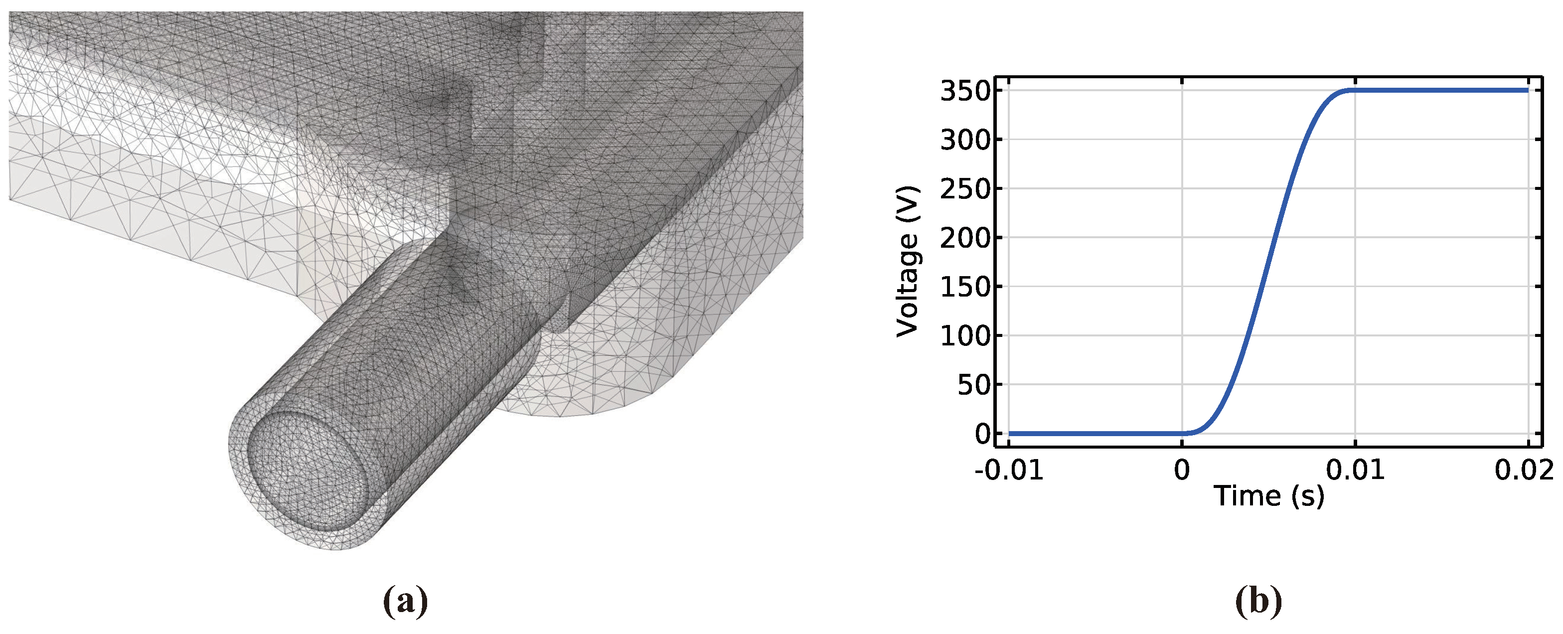
4.1. Simulation Setup

The comprehensive analysis of the electric, thermal, and fluidic behaviors of the HVLH was conducted using a coupled field numerical approach with the commercial software package COMSOL Multiphysics 6.0. This method employed COMSOL’s supplementary modules such as Composite Materials, AC/DC, CFD, and Heat Transfer to address the unified partial differential equations associated with multiple energy domains. This method eliminates the need for separate solvers for different physical domains, making it particularly well suited for complex systems such as HVLH and thermoelectric devices [12,22,23,24]. In addition, COMSOL’s ability to selectively apply solvers to specific energy domains further improves computational efficiency.

Table 1. Thermomechanical properties of materials.

Material	Density (kg/m3)	Heat Capacity (J/kg·K)	Thermal Conductivity (W/m·K)	Electrical Conductivity (S/m)	Dynamic Viscosity (Pa·s)
ALDC2	–	896	167	–	–
${\mathrm{Al}}_2{\mathrm{O}}_3$	–	730	35	–	–
Ag-Pd	11,743	341	127	$9.8\times {10}^6$	–
Coolant	1070.1	3354	0.37	–	$3.2\times {10}^{-3}$

presents the thermomechanical properties of the materials that make up the heater. The data for the materials were sourced from [12], with the exception of the Ag-Pd alloy data, which were derived using the theory of the mixture [25,26].

The fluid and structural solid domains were discretized using 3D elements, while planar-layered shell elements were used for the thin composite heating layers to improve computational efficiency in the composite TFE structure [27]. Figure 2a displays the mesh elements surrounding the coolant inlet in the computational domains. To enhance visibility of internal configurations within the simulation domain, the geometry was made semi-transparent, and only the external surface was outlined with mesh elements. The discretization of the computational domains resulted in a total of 32,010,895 3D elements, with 24,856,397 elements in the fluid domain and 7,154,498 in the solid domain, along with 24,704 layered shell elements designated for thin films. Earlier research has shown that around 2.5 million elements are required to achieve precise and convergent results in CFD and CHT studies of comparable heaters [9,10,11,12]. Consequently, the number of elements used in this study is considered adequate for reliable results.

The external surfaces of the aluminum structure, except the outer cylindrical surfaces of the inlet and outlet pipes, were subjected to convective boundary conditions. These conditions included a convection coefficient of 5.0 $\mathrm{W}/{\mathrm{m}}^2·\mathrm{K}$ and an ambient temperature of 25 °$\mathrm{C}$. The inlet and outlet pipes were presumed to be insulated by the surrounding plastic tubes that carry the coolant. The boundary conditions for the coolant entry were established with a temperature of 25 °$\mathrm{C}$ and flow rates of 5, 10, 15, and 20 L per minute (LPM). The input voltage was set to produce a sigmoid-like step signal, which increased from 0 to 350 V in 0.01 s in a smooth manner, as depicted in Figure 2b. A transient heat transfer study was conducted over a period of 60 s, with data recorded at one-second intervals.

The simulation was carried out in two primary computational phases. Initially, a CFD analysis was conducted to derive numerical solutions for steady-state turbulent flow employing the SST $k-\omega$ method. Subsequently, a dynamic conjugate heat transfer analysis was executed, considering the influences of the electric field and Joule heating. To guarantee the safe and efficient functioning of the HVLH, it is crucial to first activate the pump to circulate the working fluid prior to applying voltage to the heating element. Omitting this step can cause the internal fluid to vaporize from heat, resulting in increased pressure that could lead to a leakage of coolant in the heater joints or, in severe cases, to an explosion. Hence, it is reasonable to establish the flow field under steady-state conditions before performing the electro-thermal analysis in transient mode to simulate the heater’s real operating conditions. This methodology effectively captures the complex interplay between electrical, thermal, and fluid dynamics factors, thus providing a thorough understanding of the HVLH’s performance across various operational conditions. This technique provides in-depth knowledge that is essential for refining the heater’s design and improving its operational efficiency.

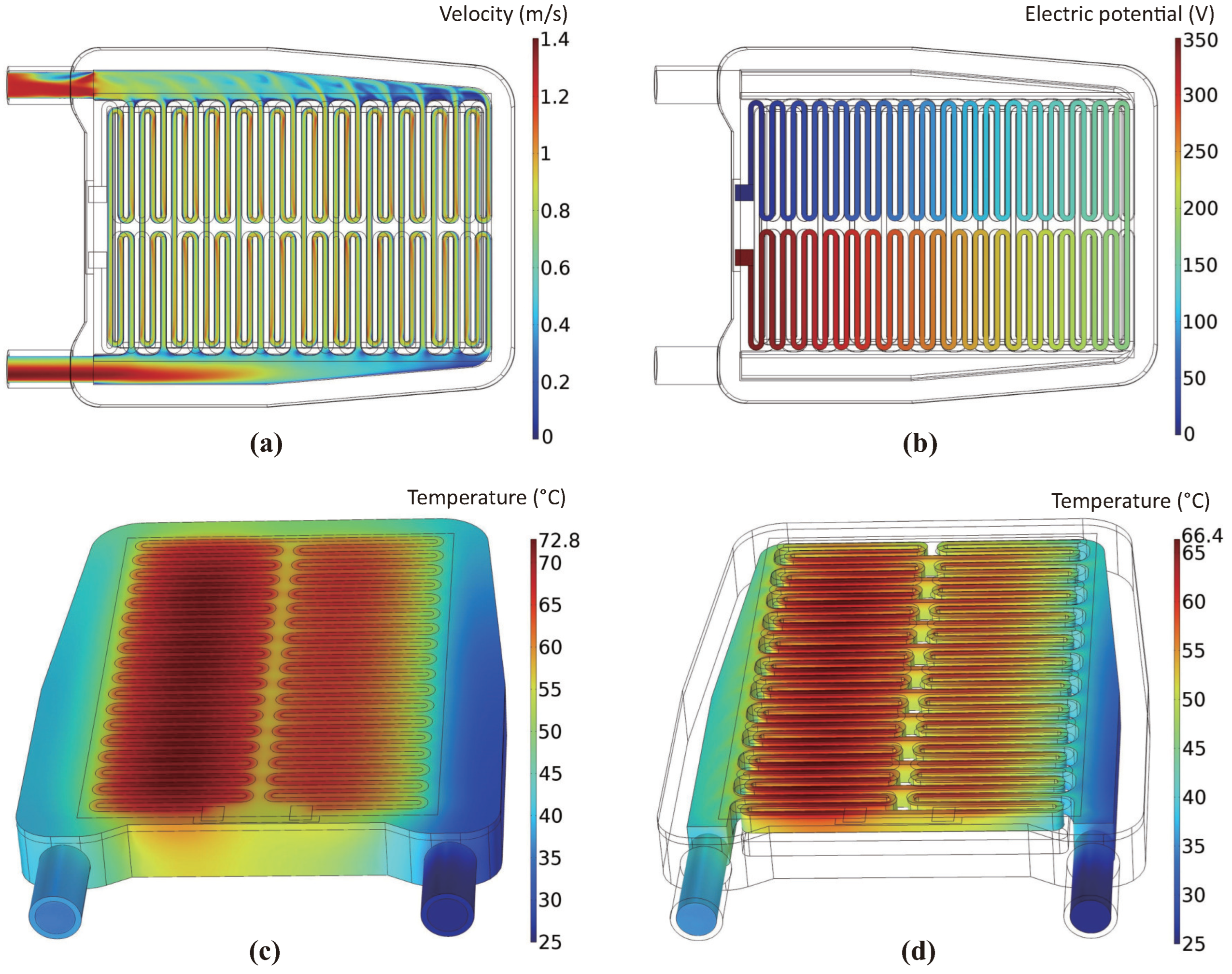
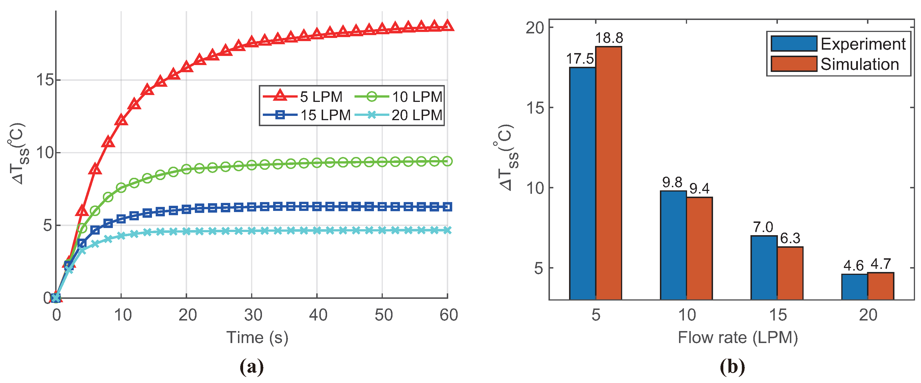
4.2. Simulation Results

Based on the simulation configuration described in Section 4.1, electro–thermo–fluidic simulations were performed under four distinct flow rate scenarios (namely, 5, 10, 15, and 20 LPM). The simulation results include the steady-state flow field, as well as the transient electric and temperature fields over a 60 s duration. The electric field reached saturation immediately after the step input was applied. However, the temperature field showed a transient response for a certain period before reaching steady-state behavior. This was due to the high heat capacity and low thermal conductivity of the fluid compared to that of the solid.

Figure 3 depicts the post-processed simulation graphics for the flow rate case of 10 LPM, which is equivalent to $1.67\times {10}^{-4}{\mathrm{m}}^3/\mathrm{s}$. Figure 3a shows a color contour plot of the velocity field in a cross-section at the middle height of the serpentine channel. The coolant enters through a single-channel inlet and flows in parallel through twelve symmetric serpentine branches within the heater body. In the last two branches, furthest from the inlet and subject to reduced hydraulic pressure, the flow speed decreases. However, no flow blockages have been observed in these channels. It is important to note that blocked channels could result in inadequate convective cooling during heater operation, potentially causing temperature-induced boiling, high vapor pressure, and subsequent damage or explosion of the heater. Figure 3b displays the steady-state electric potential field when a step voltage of 350 V is applied to the screen-printed TFE along the channel walls. A consistent voltage drop is observed from the electrical input port to the ground electrode. Figure 3c,d depict the temperature distribution outside the entire heater region and the fluid region, respectively, at 60 s. With a flow rate set at 10 LPM, it was estimated that the highest temperature at the heating element reached 72.8 °$\mathrm{C}$. The average temperature in the outlet cross-section of the fluid region was determined to be 34.4 °$\mathrm{C}$, which is 9.4 °$\mathrm{C}$ above the inlet temperature of 25 °$\mathrm{C}$.

Figure 4 displays both the transinet and steady-state data for the temperature difference, $\Delta T_{ss}$, between the inlet and the outlet derived from simulations in four LPM scenarios. Figure 4a illustrates the transient behavior of $\Delta T_{ss}$, correlating it with the coolant flow rate through the symmetric serpentine channel. Applying a 350 V DC voltage to the TFE generates thermal energy which is transferred through the aluminum wall, resulting in an increase in the outlet fluid temperature. As the fluid velocity increases, more fluid volume is subjected to heat transfer from the solid region to the fluid region. This results in a decrease in heat exchange per unit volume of the fluid and consequently leads to a lower $\Delta T_{ss}$. On the other hand, with an increase in the flow rate, the rate of convective heat transfer increases, resulting in a more rapid initial change in $\Delta T_{ss}$ and a reduced duration to achieve steady state. Figure 4b presents a bar chart comparison of the $\Delta T_{ss}$ values measured experimentally, as cited in [28], versus those obtained from the simulations in this study. The discrepancy between the experimental and simulation values ranges from 1.4% to 10.5%. Considering that higher flow velocities induce greater turbulence, which may increase the measurement errors with an immersion temperature probe, it is justifiable to claim that the simulation results closely replicate the experimental data.

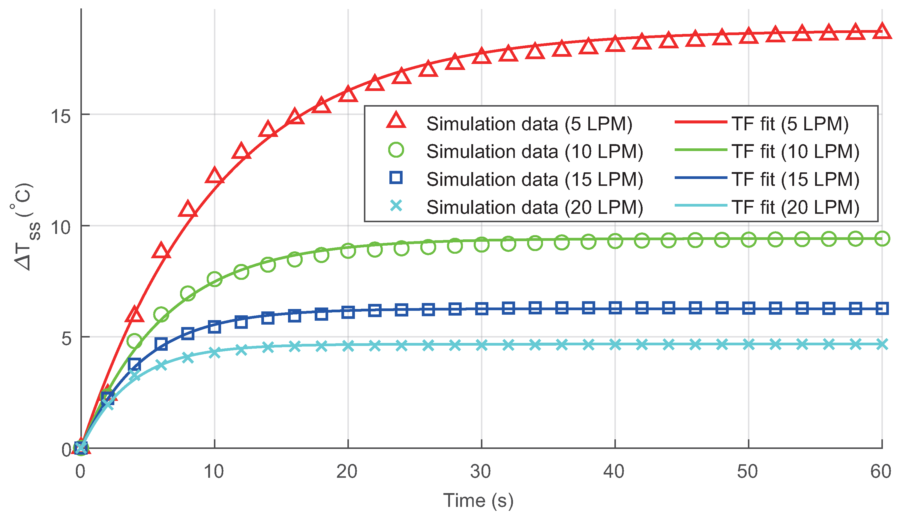
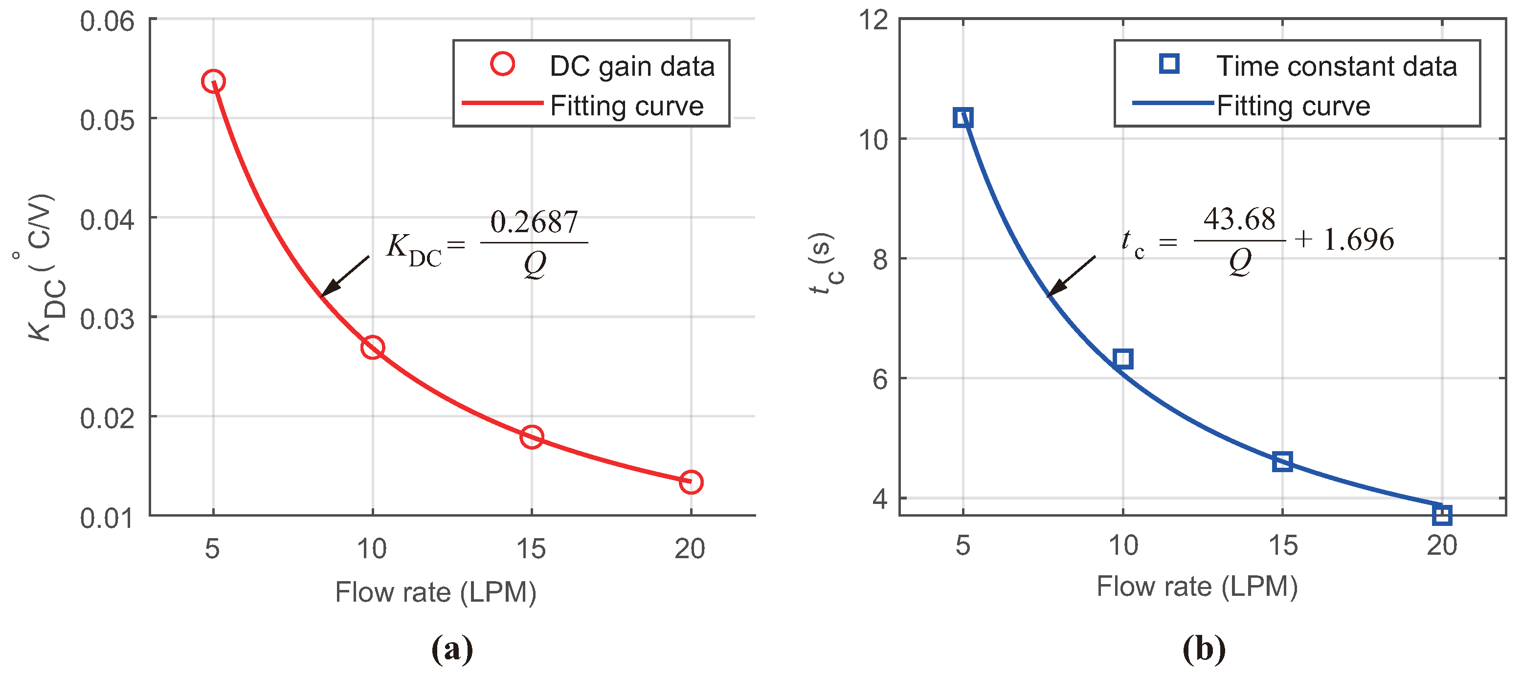
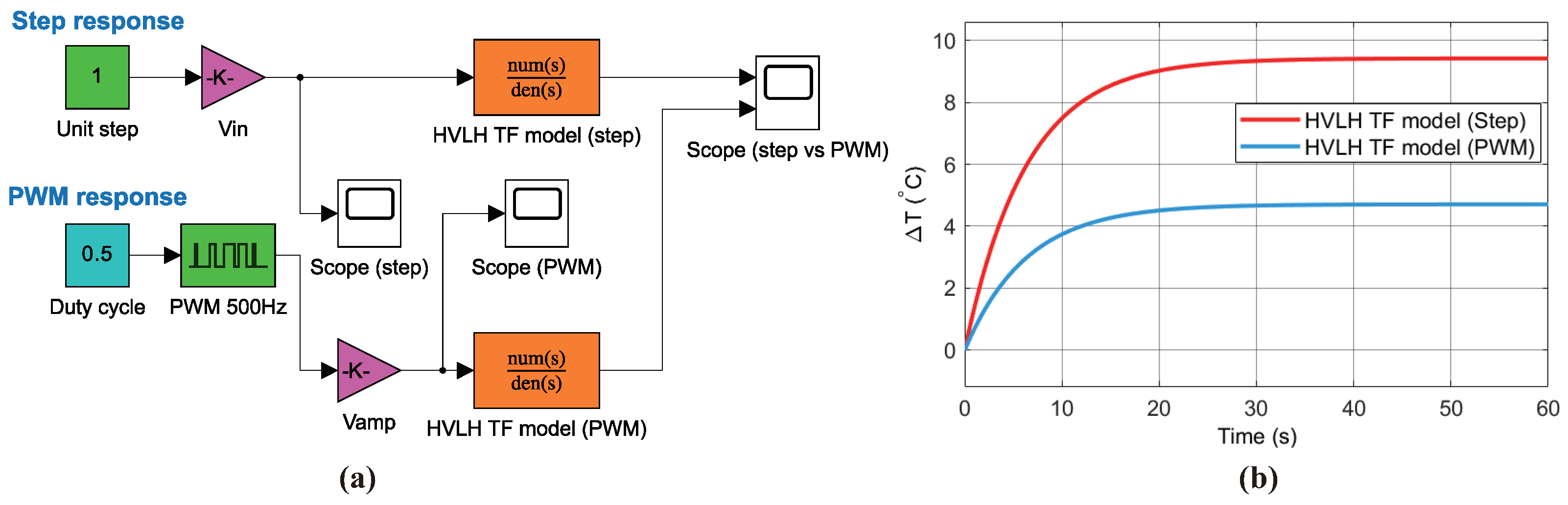
5. Transfer Function Modeling and Discussion

Previous research on the commercialization of HVLH [7,8] along with computer-aided engineering (CAE) investigations on the performance and design of products [9,10,11,12] have focused mainly on the advancement of the heater system itself. On the other hand, block diagram modeling approaches have been used to develop and implement HVLH control strategies at the system level, particularly when incorporated into EV or PHEV HVAC modules [13,14,15,16]. For this purpose, it is necessary to model the transfer function of the HVLH block. This section outlines how to derive the transfer function for HVLH using the time-dependent data collected from the simulations detailed in Section 4.2, which facilitates the system modeling of the HVAC system.

The differential energy balance equation, characterizing heat transfer phenomena, is represented as a first-order differential equation where temperature acts as a state variable, as evident from Equation (3). This inherent characteristic leads the whole heating unit to exhibit a typical dynamic behavior of a first-order linear time-invariant (LTI) system. According to the principles of modeling and control theory [29], the time-domain representation of the step response for a first-order dynamic system is expressed as follows:

$$\Delta T\left(t\right)=\left(1-e^{-\frac{t}{t_c}}\right)\Delta T_{\mathrm{ss}}$$

(6)

where $\Delta T$ denotes the increase in coolant temperature from the inlet to the outlet and $t_c$ is the time constant defining the response speed of a first-order LTI system.

The corresponding transfer function (TF) for the step response, as expressed in Equation (6), is presented as:

$$\mathrm{TF}=\frac{\Delta T\left(s\right)}{V_{\mathrm{in}}}=\frac{K_{\mathrm{DC}}}{t_{c}s+1}$$

(7)

where $\Delta T\left(s\right)$ represents the Laplace transform of $\Delta T\left(t\right)$, $V_{\mathrm{in}}$ indicates the amplitude of the input voltage, and $K_{\mathrm{DC}}$ is defined as the direct current (DC) gain, representing the proportion of the steady-state temperature difference to the step input amplitude as follows:

$$K_{\mathrm{DC}}=\frac{\Delta T_{ss}}{V_{\mathrm{in}}}$$

(8)

The control theory states that for first-order systems characterized by the transfer function in Equation (7), the rise time for an increase from 10% to 90% is given by $t_r=2.2t_c$, and the settling time to reach 99% is $t_s=4.6t_c$ [29].

Table 2. Transfer function model parameters.

Flow Rate (LPM)	${\mathit{K}}_{\mathbf{DC}}$ (°$\mathbf{C}/\mathbf{V}$)	${\mathit{t}}_{\mathit{c}}$ (s)	${\mathit{t}}_{\mathit{r}}$ (s)	${\mathit{t}}_{\mathit{s}}$ (s)
5	0.0537	10.3	22.8	47.6
10	0.0269	6.32	13.9	29.1
15	0.0179	4.61	10.1	21.2
20	0.0133	3.71	8.16	17.1

presents the DC gain, time constant, rise time, and settling time, which are derived from the regression analysis of the time-dependent simulation data corresponding to the four volume flow rates shown in Figure 4 based on Equation (7).

Figure 5 displays the results of the transfer function modeling alongside the results of the time-dependent electro–thermo–fluidic simulations. It confirms that the modeling results, which assume a first-order dynamic system, are in good agreement with the simulation data across all four volume flow rates.

To investigate the functional relationship between the volume flow rate Q and two key parameters of the transfer function, specifically the DC gain $K_{\mathrm{DC}}$ and the time constant $t_c$, additional regression analysis was performed using the data presented in Table 2. At a flow rate of zero, the heat energy constantly released from the TFE is not adequately dissipated by convective cooling, leading to significantly elevated levels of $K_{\mathrm{DC}}$ and $t_c$. In contrast, when the flow rate approaches infinity, the constrained heat energy is quickly conveyed due to the exceedingly high volume flow rate, resulting in significantly reduced levels of $K_{\mathrm{DC}}$ and $t_c$. Taking into account these tendencies, the fitting curve for the regression analysis was selected as an inversely proportional function of volume flow rate Q, defined by a coefficient a and a constant b, as follows:

$$f\left(Q\right)=\frac{a}{Q}+b$$

(9)

Figure 6 shows the results of the regression analysis applied to the parameter data of the transfer function, using a fitting curve described by Equation (9), accompanied by the respective regression functions. The fitting curves for $K_{\mathrm{DC}}$ and $t_c$ are observed to align closely with the original data.

The following equations explicitly represent the transfer function, incorporating Q as a parameter, derived from the regression analysis results for $K_{\mathrm{DC}}$ and $t_c$ depicted in Figure 6:

$$\mathrm{TF}(s;Q)=\frac{0.2687}{\left(1.969Q+43.68\right)s+Q}$$

(10)

Figure 7 shows an example of the block diagram model along with its dynamic analysis results, derived from the transfer function formulated by successive simulation, modeling, and regression analysis of the symmetric serpentine-type HVLH schematic, illustrated in Figure 1. The block diagram example shown in Figure 7a was established to analyze the step response to a 350 V voltage and to explore the performance of the popular PWM control technique [30], which is noted for its effectiveness in managing and mitigating overheating in sustained high-voltage environments. Figure 7b shows the HVLH response to a step input signal, equivalent to a PWM signal in a full duty cycle of 100%, and predicts the transient evolution of $\Delta T$ in a lower duty cycle of 50%. Upon integrating the HVLH as an electric heating component within an HVAC system, the insights gained from the transfer function modeling, as detailed in this study, are crucial for developing control strategies at the system-wide level and for predicting heater performance through block diagram modeling techniques.

6. Conclusions

This study presents a comprehensive modeling and simulation approach for high-voltage layer heaters used in electric vehicles, focusing on the transient electro–thermo–fluidic behavior and the derivation of an accurate transfer function. The key findings of this research are summarized as follows:

• This study represents the first attempt to model and simulate the HVLH by separately modeling the conductive heating layer in the electric domain, thereby calculating Joule heating and analyzing transient conjugate heat transfer. This approach improves the accuracy of predicting the thermal performance and power consumption of HVLHs.
• In addition, this research is pioneering in the modeling of the transfer function of the HVLH component, enabling its integration into system-level HVAC modeling. The derived transfer function is essential for the development and implementation of control strategies for electric vehicle heating systems.
• The results of the regression analysis for the transfer function and its parameters demonstrate a high degree of precision in reproducing the simulation data. This accurate correlation underscores the reliability of the transfer function model and its prospective usefulness in forecasting the performance of HVAC at the system level.

This research significantly advances the development and management of heating systems in electric vehicles by presenting a thorough methodology for modeling and simulation applicable across different HVAC contexts. This study contributes to the design and enhancement of HVLHs while also promoting the widespread adoption of effective heating solutions within the fast-growing electric vehicle sector. Potential future research may focus on the development of new HVLH models that feature modified flow paths and TFE configurations. Furthermore, comprehensive dynamic modeling and analysis of the entire HVAC system, including HVLH, will be performed to continue the validation and improvement of the transfer function model, thus increasing its practical utility in real-world applications.

References

1. Li, B.; Kuo, H.; Wang, X.; Chen, Y.; Wang, Y.; Gerada, D.; Worall, S.; Stone, I.; Yan, Y. Thermal Management of Electrified Propulsion System for Low-Carbon Vehicles. Automot. Innov. 2020, 3, 299–316. [Google Scholar] [CrossRef]
2. Lei, S.; Xin, S.; Liu, S. Separate and Integrated Thermal Management Solutions for Electric Vehicles: A Review. J. Power Sources 2022, 550, 232133. [Google Scholar] [CrossRef]
3. Park, M.H.; Kim, S.C. Heating Performance Characteristics of High-Voltage PTC Heater for an Electric Vehicle. Energies 2017, 10, 1494. [Google Scholar] [CrossRef]
4. Park, M.H.; Kim, S.C. Effects of Geometric Parameters and Operating Conditions on the Performance of a High-Voltage PTC Heater for an Electric Vehicle. Appl. Therm. Eng. 2018, 143, 1023–1033. [Google Scholar] [CrossRef]
5. Shin, Y.H.; Ahn, S.K.; Kim, S.C. Performance Characteristics of PTC Elements for an Electric Vehicle Heating System. Energies 2016, 9, 813. [Google Scholar] [CrossRef]
6. Paunović, V.; Mitić, V.; Đorđević, M.; Prijić, Z. Electrical Properties of Rare Earth Doped BaTiO3 Ceramics. In Proceedings of the 2017 IEEE 30th International Conference on Microelectronics (MIEL), Nis, Serbia, 9–11 October 2017; pp. 183–186. [Google Scholar] [CrossRef]
7. Cap, C.; Hainzlmaier, C. Layer Heater for Electric Vehicles. ATZ Worldw. 2013, 115, 16–19. [Google Scholar] [CrossRef]
8. Stifel, T. Optimization and Protection of Traction Batteries with an HV Coolant Heater. ATZ Worldw. 2021, 123, 44–47. [Google Scholar] [CrossRef]
9. Dong, F.; Feng, Y.; Wang, Z.; Ni, J. Effects on Thermal Performance Enhancement of Pin-Fin Structures for Insulated Gate Bipolar Transistor (IGBT) Cooling in High Voltage Heater System. Int. J. Therm. Sci. 2019, 146, 106106. [Google Scholar] [CrossRef]
10. Dong, F.; Wang, Z.; Feng, Y.; Ni, J. Numerical Study on Flow and Heat Transfer Performance of Serpentine Parallel Flow Channels in a High Voltage Heater System. Therm. Sci. 2022, 26, 735–752. [Google Scholar] [CrossRef]
11. Son, K.J. Thermo-Fluid Simulation for Flow Channel Design of 7 kW High-Voltage Heater for Electric Vehicles. J. Korea Converg. Soc. 2022, 13, 191–196. [Google Scholar] [CrossRef]
12. Son, K.J. Optimal Power Distribution of High-Voltage Coolant Heater for Electric Vehicles through Electro-Thermofluidic Simulations. Int. J. Automot. Technol. 2023, 24, 995–1003. [Google Scholar] [CrossRef]
13. Bellocchi, S.; Leo Guizzi, G.; Manno, M.; Salvatori, M.; Zaccagnini, A. Reversible Heat Pump HVAC System with Regenerative Heat Exchanger for Electric Vehicles: Analysis of Its Impact on Driving Range. Appl. Therm. Eng. 2018, 129, 290–305. [Google Scholar] [CrossRef]
14. Basciotti, D.; Dvorak, D.; Gellai, I. A Novel Methodology for Evaluating the Impact of Energy Efficiency Measures on the Cabin Thermal Comfort of Electric Vehicles. Energies 2020, 13, 3872. [Google Scholar] [CrossRef]
15. Dvorak, D.; Basciotti, D.; Gellai, I. Demand-Based Control Design for Efficient Heat Pump Operation of Electric Vehicles. Energies 2020, 13, 5440. [Google Scholar] [CrossRef]
16. Kulkarni, A.; Brandes, G.; Rahman, A.; Paul, S. A Numerical Model to Evaluate the HVAC Power Demand of Electric Vehicles. IEEE Access 2022, 10, 96239–96248. [Google Scholar] [CrossRef]
17. Menter, F.R. Two-Equation Eddy-Viscosity Turbulence Models for Engineering Applications. AIAA J. 1994, 32, 1598–1605. [Google Scholar] [CrossRef]
18. Menter, F.R.; Kuntz, M.; Langtry, R. Ten Years of Industrial Experience with the SST Turbulence Model. Turbul. Heat Mass Transf. 2003, 4, 625–632. [Google Scholar]
19. Speziale, C.G.; Abid, R.; Anderson, E.C. Critical Evaluation of Two-Equation Models for near-Wall Turbulence. AIAA J. 1992, 30, 324–331. [Google Scholar] [CrossRef]
20. Rivero, E.P.; Granados, P.; Rivera, F.F.; Cruz, M.; González, I. Mass Transfer Modeling and Simulation at a Rotating Cylinder Electrode (RCE) Reactor under Turbulent Flow for Copper Recovery. Chem. Eng. Sci. 2010, 65, 3042–3049. [Google Scholar] [CrossRef]
21. Weigand, B.; Ferguson, J.R.; Crawford, M.E. An Extended Kays and Crawford Turbulent Prandtl Number Model. Int. J. Heat Mass Transf. 1997, 40, 4191–4196. [Google Scholar] [CrossRef]
22. Luo, D.; Wang, R.; Yan, Y.; Sun, Z.; Zhou, W.; Ding, R. Comparison of Different Fluid-Thermal-Electric Multiphysics Modeling Approaches for Thermoelectric Generator Systems. Renew. Energy 2021, 180, 1266–1277. [Google Scholar] [CrossRef]
23. Jouhara, H.; Żabnieńska-Góra, A.; Khordehgah, N.; Doraghi, Q.; Ahmad, L.; Norman, L.; Axcell, B.; Wrobel, L.; Dai, S. Thermoelectric Generator (TEG) Technologies and Applications. Int. J. Thermofluids 2021, 9, 100063. [Google Scholar] [CrossRef]
24. Son, K.J. Thermo-Electro-Fluidic Simulation Study of Impact of Blower Motor Heat on Performance of Peltier Cooler for Protective Clothing. Energies 2023, 16, 4052. [Google Scholar] [CrossRef]
25. Drumheller, D.S. Hypervelocity Impact of Mixtures. Int. J. Impact Eng. 1987, 5, 261–268. [Google Scholar] [CrossRef]
26. Son, K.J.; Fahrenthold, E.P. Impact Dynamics Simulation for Magnetorheological Fluid Saturated Fabric Barriers. J. Comput. Nonlinear Dyn. 2024, 19, 061002. [Google Scholar] [CrossRef]
27. Zhang, X.; Jane Wang, Q.; He, T.; Liu, Y.; Li, Z.; Kim, H.J.; Pack, S. Fully Coupled Thermo-Viscoelastic (TVE) Contact Modeling of Layered Materials Considering Frictional and Viscoelastic Heating. Tribol. Int. 2022, 170, 107506. [Google Scholar] [CrossRef]
28. Kwon, B.W. Development of 7 kW-Class Thick Film Resistance Heating Electric Heater (10% Weight Reduction) for Lighter Green Vehicle Cooling, Heating and HVAC System; Final Project Report (Written in Korean) No. P0017526; Korean Ministry of Trade, Industry and Energy (MOTIE): Sejong, Republic of Korea, 2023.
29. Franlkin, G.F.; Powell, J.D.; Emami-Naeini, A. Feedback Control of Dynamic Systems, 8th ed.; Higher Education, Inc.: Upper Saddle River, NJ, USA, 2018; pp. 137–142. [Google Scholar]
30. Shin, Y.H.; Sim, S.; Kim, S.C. Performance Characteristics of a Modularized and Integrated PTC Heating System for an Electric Vehicle. Energies 2016, 9, 18. [Google Scholar] [CrossRef]
Figure 1. HVLH schematic diagram: (a) disassembled illustration of heater consisting of main body with serpentine walls and cover plate with screen-printed heating layer; (b) heater body including symmetric serpentine flow channels with twelve branches in parallel.
Energies 17 02935 g001
Figure 2. Preprocessing of electro–thermo–fluidic simulation: (a) meshed elements zoomed-in around the coolant inlet and (b) Sigmoid-based step voltage input function.
Energies 17 02935 g002
Figure 3. Simulation results for inlet flow rate of 10 LPM at 60 s: (a) steady-state velocity magnitude contour plot at the middle cross-section of serpentine flow channels; (b) electric potential contour plot on the conductive heating layer; (c) temperature contour plot on the solid surface; (d) temperature contour plot on the fluid surface.
Energies 17 02935 g003
Figure 4. Time-dependent thermal analysis results: (a) temperature difference versus time curve for different coolant flow rates, with data points collected every 2 s; (b) bar graphs comparing simulated and experimental results for steady-state temperature increase from inlet to outlet.
Energies 17 02935 g004
Figure 5. Transfer function curves fitted against simulation data for various LPMs.
Energies 17 02935 g005
Figure 6. Results from curve fitting of transfer function parameters for (a) steady-state gain and (b) time constant.
Energies 17 02935 g006
Figure 7. PWM control of high-voltage heat using the transfer function model: (a) block diagram schematic; (b) step response versus PWM response curves.
Energies 17 02935 g007