Bi-Level Planning of Electric Vehicle Charging Stations Considering Spatial–Temporal Distribution Characteristics of Charging Loads in Uncertain Environments

Abstract

With the increase in the number of distributed energy resources (DERs) and electric vehicles (EVs), it is particularly important to solve the problem of EV charging station siting and capacity determination under the distribution network considering a large proportion of DERs. This paper proposes a bi-level planning model for EV charging stations that takes into account the characteristics of the spatial–temporal distribution of charging loads under an uncertain environment. First, the Origin–Destination (OD) matrix analysis method and the real-time Dijkstra dynamic path search algorithm are introduced and combined with the Larin Hypercube Sampling (LHS) method to establish the EV charging load prediction model considering the spatial and temporal distribution characteristics. Second, the upper objective function with the objective of minimizing the cost of EV charging station planning and user charging behavior is constructed, while the lower objective function with the objective of minimizing the cost of distribution network operation and carbon emission cost considering the uncertainty of wind power and photovoltaics is constructed. The constraints of the lower-layer objective function are transformed into the upper-layer objective function through Karush–Kuhn–Tucker (KKT) conditions, the optimal location and capacity of charging stations are finally determined, and the model of EV charging station siting and capacity determination is established. Finally, the validity of the model was verified by planning the coupled IEEE 33-node distribution network with the traffic road map of a city in southeastern South Dakota, USA.

1. Introduction

At present, the problems of global energy shortage and greenhouse gas emissions are becoming increasingly significant. As a large country in terms of population and manufacturing, China’s energy consumption and carbon dioxide emissions cannot be ignored. In response to this problem, China has put forward the dual-carbon goals of “carbon peaking” and “carbon neutrality”. In recent years, the EV, with its excellent characteristics of environmental protection and energy saving, has great potential to become an ideal substitute for fuel vehicles in the future and will face a wide range of applications. As the basic supporting facilities of EV, affecting the level of EV application, scientific and reasonable planning for charging stations can not only reduce the investment and construction costs, and mitigate the impact on the distribution network caused by a large number of EV access, but also allow EV users to enjoy convenient charging services [1,2,3,4,5]. At the same time, the access of a large number of DERs of various types to the distribution grid leads to changes in the distribution structure and the operation mode of the grid, and the inherent uncertainty of wind power and photovoltaics creates a huge challenge to the safe and stable operation of the grid [6,7,8,9,10,11]. Therefore, studying the siting and capacity-setting of EV charging stations while considering the uncertainties of wind power and PV can effectively mitigate the adverse impacts on the stability and economy of grid operation due to the fluctuations arising from the access of DERs and EVs to the distribution grid.

Forecasting EV charging load demand is a prerequisite for proper charging station planning. Considering the effects of high uncertainty in weather, traffic, and driver behavior, Wu et al. [12] proposed an optimal parameter prediction method that can improve the prediction accuracy of charging demand of EVs in MG. Zhuang et al. [13] combined a multi-source information architecture consisting of an information layer, an algorithm layer, and a model layer to predict the loads of the EV control system in the region. They also proposed a decision-making method for EV charging stations based on prospect theory. Feng et al. [14] proposed a new EV charging load prediction model considering traffic conditions and ambient temperature: a traffic network topology and a speed flow model were established to accurately simulate the driving state of EVs in a real road network, and the power consumption per unit kilometer of an EV was calculated by taking into account the effects of temperature and vehicle speed on power consumption. In order to address the short-term and long-term prediction of EV charging loads, Koohfar et al. [15] made the first attempt to use the Transformer model to predict EV charging demand and compare the performance with the RMSE model and the MAE model. Huang et al. [16] analyzed the spatial and temporal correlation of multi-node charging loads under the joint charging scenarios of prediction and historical days to effectively predict the spatial and temporal distributions of electric vehicle charging loads and proposed a multi-node charging loads joint anti-generation interval prediction method considering the spatial correlation of the charging loads among nodes. Hu et al. [17] proposed a short-term probabilistic charging demand prediction model for estimating the future charging demand at charging stations 15 min in advance based on the self-attention-based theory of mind for machines (SAMToM), which takes into account the user’s historical charging habits and the current trend of charging demand changes. In order to study the centralized charging problem of interchangeable EVs, He et al. [18] established a model of the driving energy consumption process and range of EVs based on the road topology model and established a spatial–temporal distribution model of the loads of interchangeable EVs by analyzing the travel demand of users.

Currently, the siting and capacity allocation of EV charging stations is still a complicated issue. Site selection requires comprehensive consideration of the impact of a variety of factors, while the charging station capacity configuration needs to be adapted to local conditions. Zhang et al. [19] introduced a multi-objective optimization method based on the NSGA-II algorithm to determine the location of EV charging stations by considering multiple variables in the planning of charging stations with the optimization objectives of maximizing the system benefits and maximizing the minimum coverage of charging demand level by charging stations. By combining EV charging data and driving chain to obtain more accurate charging load data, Yin et al. [20] established an optimal allocation model with the goal of optimal network loss and introduced the second-order cone relaxation technique to solve the nonconvexity. Jiang et al. [21] proposed a novel EV charging station layout optimization method based on power system flexibility, which not only considers EV charging behavior and sequential charging demand but also considers the impact on the power system. Schoenberg et al. [22] broke down the charging and energy consumption models for five types of electric vehicles in the market and found suitable locations for the installation of slow- and fast-charging stations by analyzing the user’s daily journeys as well as coordinating the charging needs using a centralized charging station database. Wang et al. [23] proposed a hybrid approach based on a Bayesian network with the best–worst method (BN-BWM) and geographic information system (GIS) to solve the problem of siting and sizing of electric vehicles, and the results proved that the method is highly operable and convincing in terms of accuracy. In order to solve the problem of short charging cycles, Wu et al. [24] introduced renewable energy sources and investigated the impact of extremely fast-charging stations on the distribution network. Zhang et al. [25] proposed a three-time charging station siting and capacity model based on high-resolution spatial and temporal charging demand distribution based on the M/M/c/N charging queuing theory and the actual operation data of electric vehicles in Beijing. Wang et al. [26] planned the charging station installation locations and charging station capacities using neural networks and chance constraints, taking into account the uncertainty of charging demand, and found their optimal solutions using the Dantzig–Wolfe decomposition method. Woo et al. [27] proposed a minimum genetic algorithm combining game theory and the genetic algorithm to solve the optimal charging station layout model and minimize the peak charging demand.

In addition, in the context of distributed energy uncertainty, Nasab et al. [28] used the R language to simulate wind and solar power outputs along with time series analysis, from which a large number of scenarios are generated; then, low probability scenarios are eliminated by vector distance. Xu et al. [29] used normal distribution to analyze the prediction errors of wind and solar power outputs and described their uncertainties by the trapezoidal fuzzy numerical equivalence model. Ye et al. [30] first proposed a multi-objective wind and solar power output prediction model based on a hybrid pseudo-inverse Laguerre neural network; then, they used Latin hypercubic sampling and simultaneous backward reduction for scenario generation and scenario reduction to deal with the uncertainty. Bhavsar et al. [31] proposed a hybrid data-driven and physically-based modeling forecasting paradigm to contribute to the uncertainty in wind and solar forecasts.

This paper introduces a bi-level planning model designed for EV charging stations, considering the spatial–temporal distribution of charging loads within an uncertain environment. Initially, the approach incorporates the OD matrix analysis method and real-time Dijkstra dynamic path search algorithm, integrating them with the LHS method to formulate an EV charging load prediction model that accounts for both spatial and temporal distribution characteristics. Subsequently, the upper-level objective function is formulated to minimize the cost associated with EV charging station planning and user charging behavior. Simultaneously, a lower-level objective function is constructed with the goal of minimizing the cost of distribution network operation and carbon emission cost, considering uncertainties related to wind power and photovoltaic sources. The constraints from the lower-level objective function are transformed into the upper-level objective function using KKT conditions. This process facilitates the determination of optimal charging station locations and capacities, culminating in the establishment of a comprehensive model for EV charging station siting and capacity determination. Finally, the model’s effectiveness is validated through the planning of a coupled IEEE 33-node distribution network with the traffic road map of a city in southeastern South Dakota, USA.

The structure of the remainder of the paper is as follows: Section 2 shows the EV charging load prediction. Section 3 covers a bi-level model for charging station siting and capacity determination. Section 4 uses KKT conditions to solve the bi-level model. Section 5 gives an example analysis, and Section 6 draws conclusions.

2. EV Charging Load Prediction

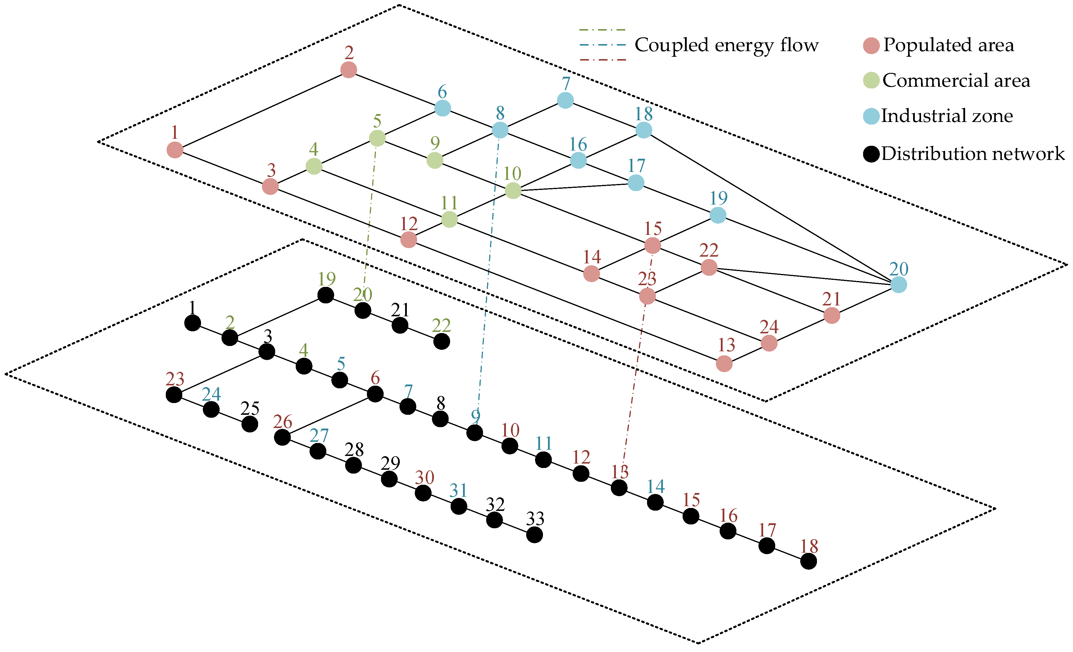
2.1. Coupling of the Road Network to the Distribution Network

As a means of transportation, the travel path of EVs will be affected by urban traffic path planning. At the same time, the user’s charging demand and charging strategy will not only be affected by the travel path but also bring security threats to the distribution network operation. Therefore, the establishment of a coupled road network–distribution network is the first condition to analyze the charging demand of EV loads. The 24-node road network–33-node distribution network coupling network is shown in Figure 1.

In order to better describe the EV travel destinations and count the distribution of charging demand, this paper focuses on three types of vehicles: private cars, cabs, and online car-hailings, and divides the 24-node road network in the above figure into three types of areas to be planned according to the functional types and load characteristics of each area of the city: the commercial area, the industrial zone, and the populated area.

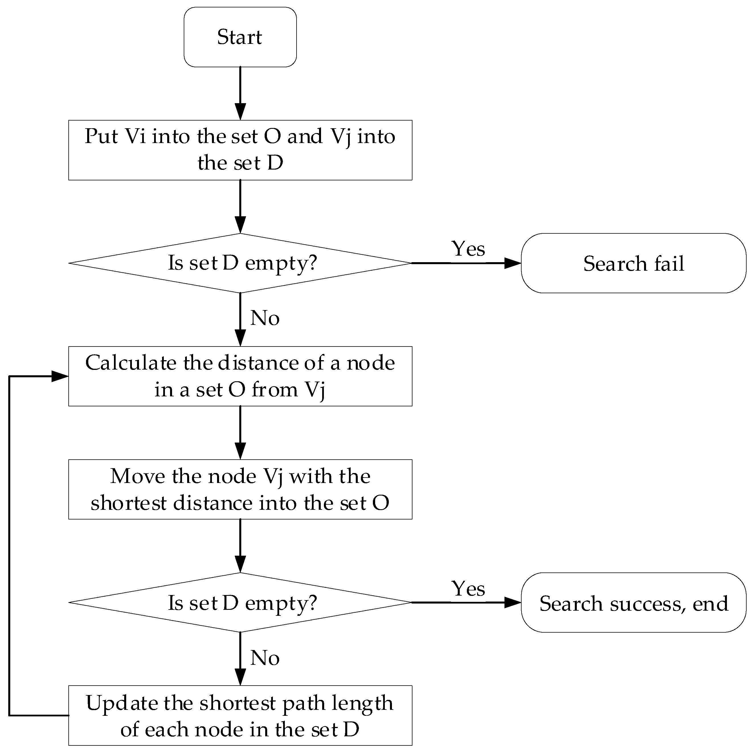
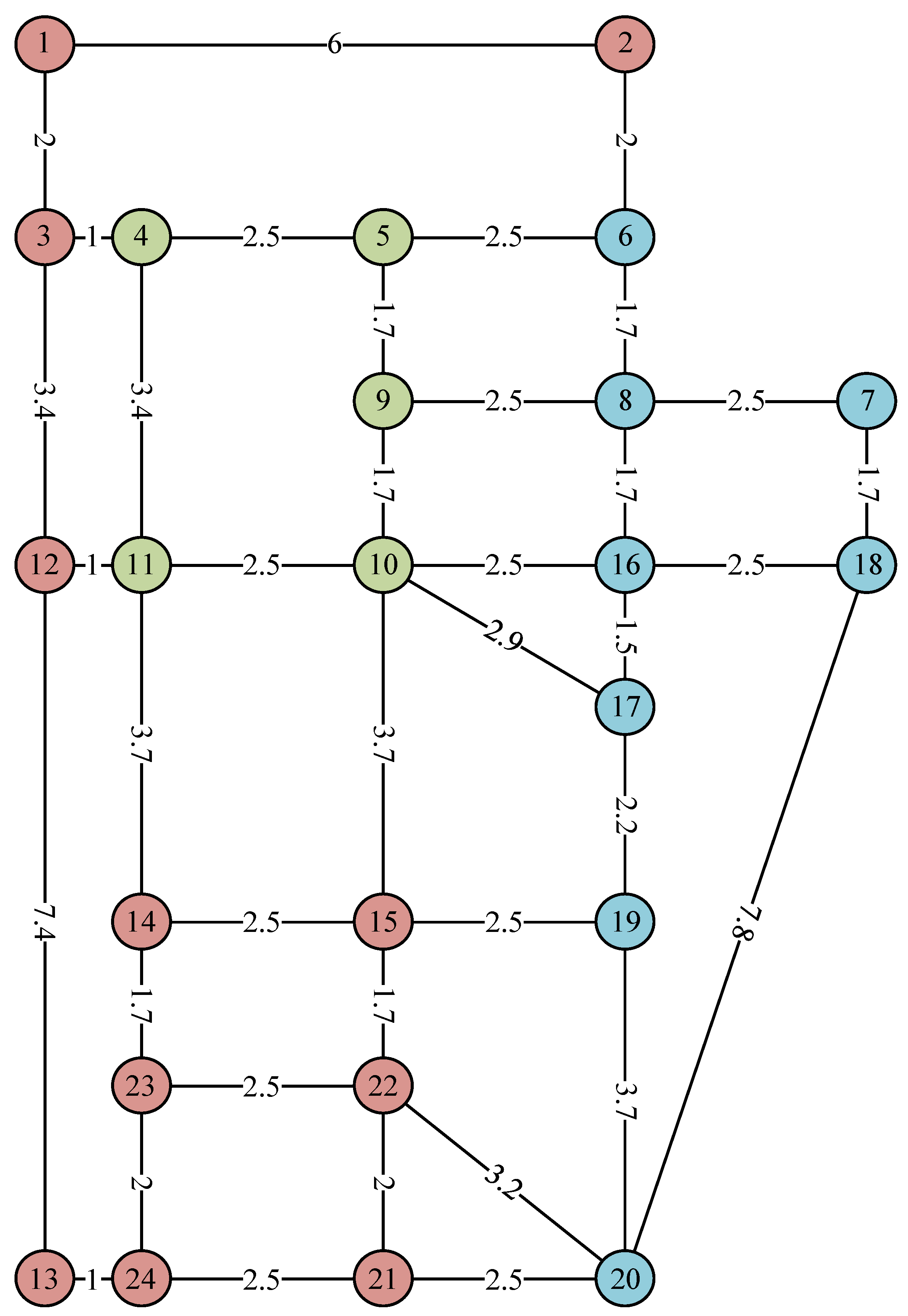
2.2. OD Matrix and Dijkstra’s Shortest Path Algorithm

The OD matrix is the volume of traffic trips from all origins to destinations in a transportation network [32]. The rows of the matrix represent traffic generation at each origin and the columns represent traffic attraction at each destination. The OD matrix ${\mathit{P}}_{m\times m}^{T,T+1}$ can be obtained by backcasting the actual traffic flow of EVs on each road segment measured by the transportation department.

$$p_{i,j}^{T,T+1}=\frac{b_{i,j}^{T,T+1}}{{\displaystyle \sum _{j=1}^m{b}_{i,j}^{T,T+1}}}, 1\le i,j\le m$$

(1)

where $m$ is the number of road nodes, the numerator denotes the number of electric vehicles starting from road network node $i$ and arriving at road network node $j$, the denominator represents the total number of electric vehicles departing from node $i$ of the road network, and $p_{i,j}^{T,T+1}$ indicates the travel probability between road network node $i$ and road network node $j$ at the moment $T$~$T+1$.

In this paper, it is assumed that cabs and internet taxis have a negligible amount of time spent at the destination. We use the LHS to sample and obtain the behavioral characteristic indexes such as initial location, time of going to work, time of going out of work, initial SOC, and driving speed of cabs and online car-hailings. Based on obtaining the OD matrix of each EV, a real-time Dijkstra algorithm is used for path guidance to search for the shortest path between ODs [33]. The flow of Dijkstra’s algorithm is shown in Figure 2, where $Vi$ stands for the starting node, $Vj$ refers to the target node, Set $O$ is used to hold unexamined nodes, and Set $D$ is used to hold the examined nodes.

2.3. Travel Chain Model

Unlike cabs and online car-hailings, electric private cars have a more regular travel pattern. Their travel destinations are more fixed and can be categorized into three types: populated area, industrial zone, and commercial area (including supermarkets, hospitals, schools, etc.), which are abbreviated as H, W, and O, respectively. The travel chain involved in this paper is shown in Figure 3. The probability distribution of the three travel trips is 52.8%, 24.1%, and 23.1%.

2.4. EV Charging Load Prediction Considering Spatial–Temporal Distribution

Before predicting the demand for charging load, it is necessary to first determine the number of various vehicle models in the city. This article uses the LHS method to sample four types of vehicle models in different proportions. After obtaining the quantity of various vehicle models, this article will separate private cars from other cars. For private cars, first use the LHS method to sample their travel chains and obtain their respective travel chains. Then, sample its initial SOC, departure time, starting location, and other behavioral characteristics indicators. For other vehicles, the sampling of the travel chain can be omitted, and the LHS method can be directly used to sample their initial SOC, departure time, starting location, and other behavioral characteristics indicators.

From Section 2.2 and Section 2.3, the behavioral characteristics indicators of private cars, cabs, and online car-hailings can be obtained; hence, their traveling status is obtained. Thus, the charging demand of the three models at each node of the road network is obtained. In this paper, the charging demand loads of the three models are modeled, and the specific flow is shown in Figure 4.

3. A Bi-Level Model for Charging Station Siting and Capacity Determination

In this paper, a bi-level planning model is developed to plan the location and capacity of electric vehicle charging stations. The upper-level model establishes an optimization model that minimizes the total cost during the planning period based on the annualized cost of the charging station and the annualized economic loss of the users. The lower model considers the uncertainty of wind power and photovoltaic and establishes an optimization model to minimize the operating cost of the distribution network with the increase in charging demand load.

3.1. Upper-Level Charging Station Planning Model

3.1.1. Upper-Level Objective Function

The upper-level objective function integrates the interests of both charging stations and EV users.

$$\min f_{upper}=f_1+f_2$$

(2)

where $f_{upper}$ shows the annualized total economic cost, $f_1$ stands for the annualized economic cost of the charging station, and $f_2$ represents the user’s annualized economic loss.

(1)

Annualized cost of the charging station

The annualized cost of the charging station $f_1$ mainly includes the annual construction cost $C_{build}$ and the annual operation and maintenance cost $C_{maint}$.

$$f_1=C_{build}+C_{maint}$$

(3)

(a)

Annual construction cost

The annual construction cost of a charging station $C_{build}$ includes the cost of the capital investment $C_{iv}$ and the cost of purchasing the charging piles $C_{pc}$.

$$C_{build}=C_{iv}+C_{pc}$$

(4)

$$C_{iv}=\frac{r_0{(1+r_0)}^y}{{(1+r_0)}^y-1}{\displaystyle \sum _{i=1}^N{C}_{iv,i}}$$

(5)

$$C_{pc}=\frac{r_0{(1+r_0)}^y}{{(1+r_0)}^y-1}{\displaystyle \sum _{i=1}^N{C}_{pc,i}}$$

(6)

where $y$ is the operating life of the charging station, $N$ refers to the number of charging stations, $C_{iv,i}$ stands for the capital investment cost of the charging station $i$, $C_{pc,i}$ stands for the purchase cost of the charging pile of the charging station $i$, and $r_0$ is the discount rate.

The purchase cost of charging piles $C_{pc,i}$ depends on the type and number of charging piles. Fast-charging piles are expensive and have high charging efficiency, while slow-charging piles have low purchase cost despite longer charging time. The specific configuration scheme of charging piles will be developed according to the charging demand characteristics of different functional areas in the city. Therefore, the purchase cost of the charging pile and the corresponding operating capacity in the charging station $i$ can be expressed in the following form:

$$C_{pc,i}=C_{fast}{N}_{fast,i,o}+C_{slow}{N}_{slow,i,o}$$

(7)

where $C_{fast}$ is the price of a single fast-charging pile, $C_{slow}$ is the price of a single slow-charging pile, $N_{fast,i,o}$ represents the number of fast-charging piles in the charging station $i$ belonging to functional area $o$, and $N_{slow,i,o}$ represents the number of fast-charging piles in the charging station $i$ belonging to functional area $o$.

(b)

Annual operation and maintenance cost

This cost includes personnel salaries, costs of equipment wear and tear, and maintenance costs. Considering the complexity of the actual annual operation and maintenance cost components, the annual operation and maintenance cost can be expressed by multiplying the annual operating capacity by a proportionality parameter.

$$C_{maint}=\left(\partial +\upsilon \right){\displaystyle \sum _{i=1}^N{C}_{cp,i}}$$

(8)

$$C_{cp,i}=365\cdot T_{day}\left(P_{fast}{N}_{fast,i,o}+P_{slow}{N}_{slow,i,o}\right)$$

(9)

where $P_{fast}$ refers to fast-charging power, $P_{slow}$ refers to slow-charging power, $T_{day}$ is average daily operating hours of a charging station, $C_{cp,i}$ represents the annual operating capacity of the charging station $i$, $\partial$ stands for personnel salary ratio parameter, and $\upsilon$ represents grid-connected cost ratio parameter.

(2)

User’s annualized economic loss

The user’s annualized economic loss $f_2$ mainly includes the cost of time lost on the way to the charging station $C_{lost}$ and the cost of driving empty on the way to the charging station $C_{empty}$.

$$f_2=C_{lost}+C_{empty}$$

(10)

(c)

Cost of time lost on the way to the charging station

$$C_{lost}=365\cdot \theta {\displaystyle \sum _{i=1}^N{\displaystyle \sum _{n=1}^{N_{c,i}}\Delta T_{i,n}}}$$

(11)

where $\theta$ is unit time cost of urban travel, $N_{c,i}$ represents the number of charging demands within the service area of the charging station $i$, and $\Delta T_{i,n}$ stands for the time from the current location to the charging station for a particular EV in need of charging.

(d)

Cost of driving empty on the way to the charging station

$$C_{empty}=365\cdot {\displaystyle \sum _{i=1}^N{\displaystyle \sum _{n=1}^{N_{c,i}}{d}_{i,n}\Delta E_{i,n}{C}_{i,chp}}}$$

(12)

where $d_{i,n}$ is the distance of EV $n$ to the charging station $i$, $\Delta E_{i,n}$ refers to average power consumption per 1 km traveled by EVs in the target area, and $C_{i,chp}$ represents average price of electricity for EV charging at charging station $i$.

3.1.2. Upper-Level Constraints

(1)

Number of Charging Stations Constraint

The number of charging stations $N$ in the area to be planned determines the economic benefits for both charging stations and users.

$$N_{\min }\le N\le N_{\max }$$

(13)

where $N_{\min }$ is minimum number of charging stations and $N_{\max }$ is maximum number of charging stations.

(2)

Charging demand constraint

In order to ensure that charging stations are able to meet the charging needs of users and to avoid the situation of supply falling short of demand, the total power of the charging stations per day is constrained to be no less than the total EV charging demand in that coverage area.

$$\left(P_{fast}{N}_{fast,i,o}+P_{slow}{N}_{slow,i,o}\right)T\ge P_{rd,i}$$

(14)

where $T$ represents 24 h a day and $P_{rd,i}$ is the total EV charging demand for charging station $i$.

(3)

Charging station distance constraint

In order to avoid the distance between EV charging stations being too far, which leads to inconvenience for users to charge, or the utilization rate of charging stations being low due to the centralized location, the distance constraints between charging stations are set as follows:

$${\displaystyle \sum _i^N{\delta }_{i,u}\ge 1}, \forall u\in S$$

(15)

where $S$ is the set of charging demand points included in the service area of each alternative charging station, $u$ denotes the set containing the charging station $i$, ${\delta }_{i,u}=1$ indicates a charging station can be installed at node $i$, and ${\delta }_{i,u}=0$ indicates that a charging station cannot be installed at node $i$.

(4)

Regional charging pile number constraint

The demand for charging services varies in different functional areas of the city. EV users generally do not stay for long in commercial areas and choose fast charging as their preferred charging method; so, the number of fast-charging piles should be higher than the number of slow-charging piles in charging stations in commercial areas. On the contrary, the number of fast-charging piles should be less than or equal to the number of slow-charging piles in charging stations in residential or industrial areas. Therefore, the constraints on the number of different types of charging piles within a charging station are set as follows:

$$N_{fast,i,o}=\tau N_{slow,i,o}, \forall o\in Y$$

(16)

where $\tau$ is a parameter for the ratio between the number of fast-charging piles and the number of slow-charging piles, and $Y$ represents the set of different regional scopes.

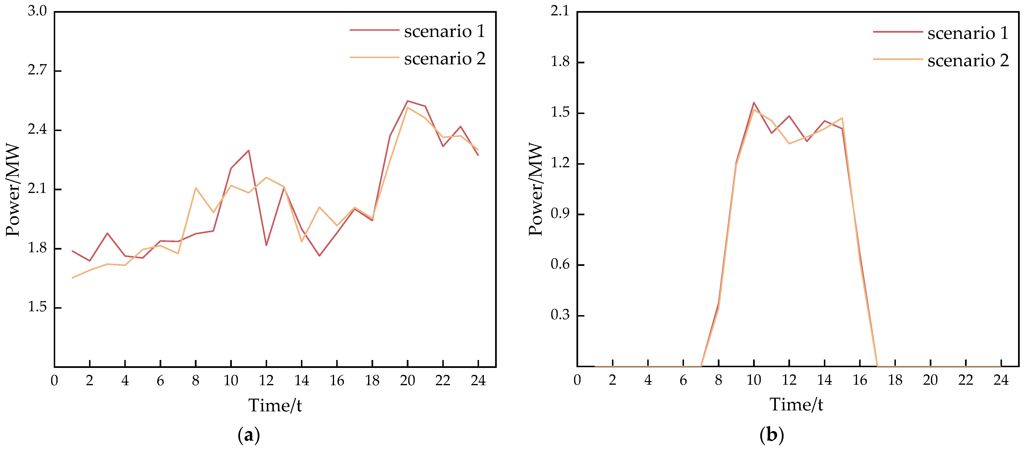
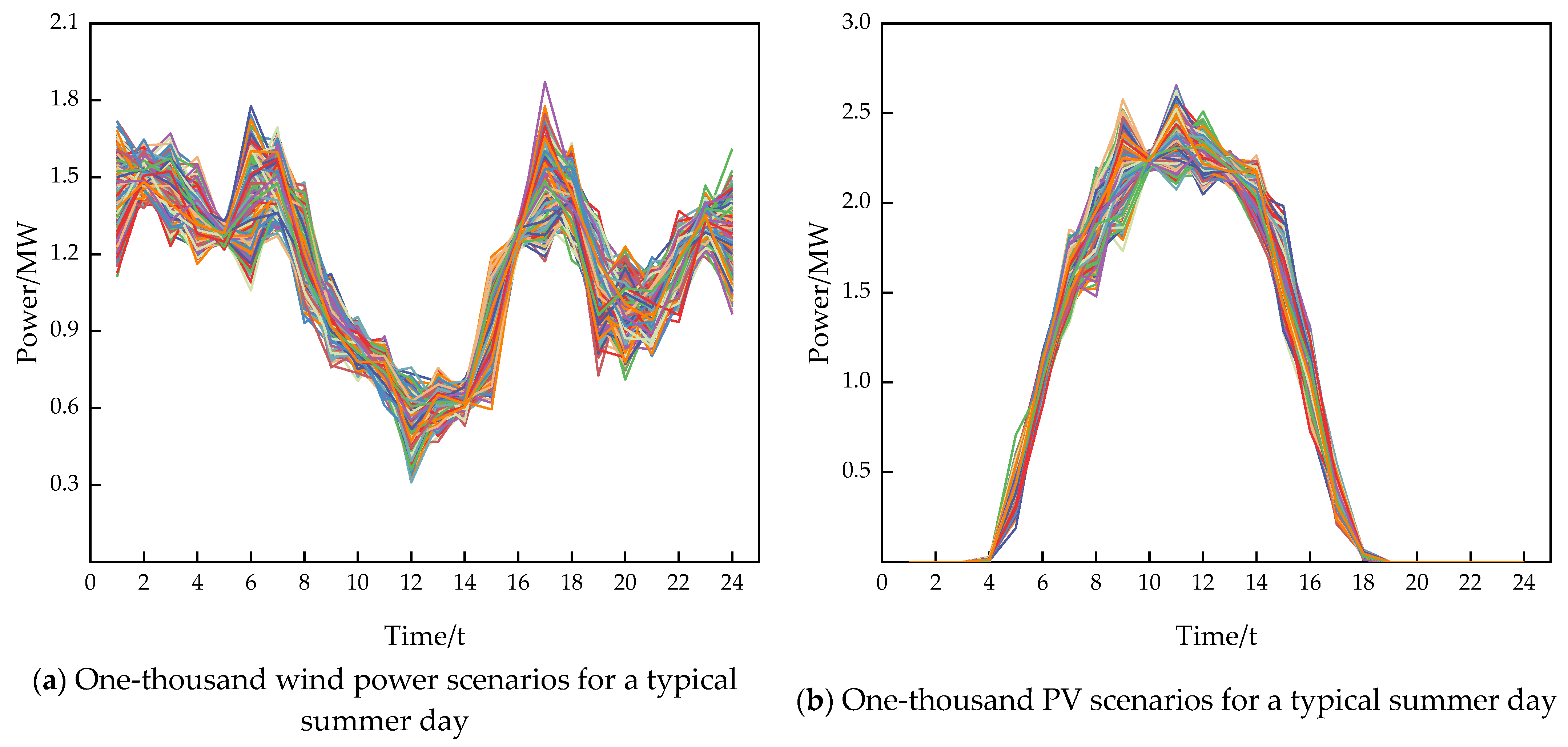
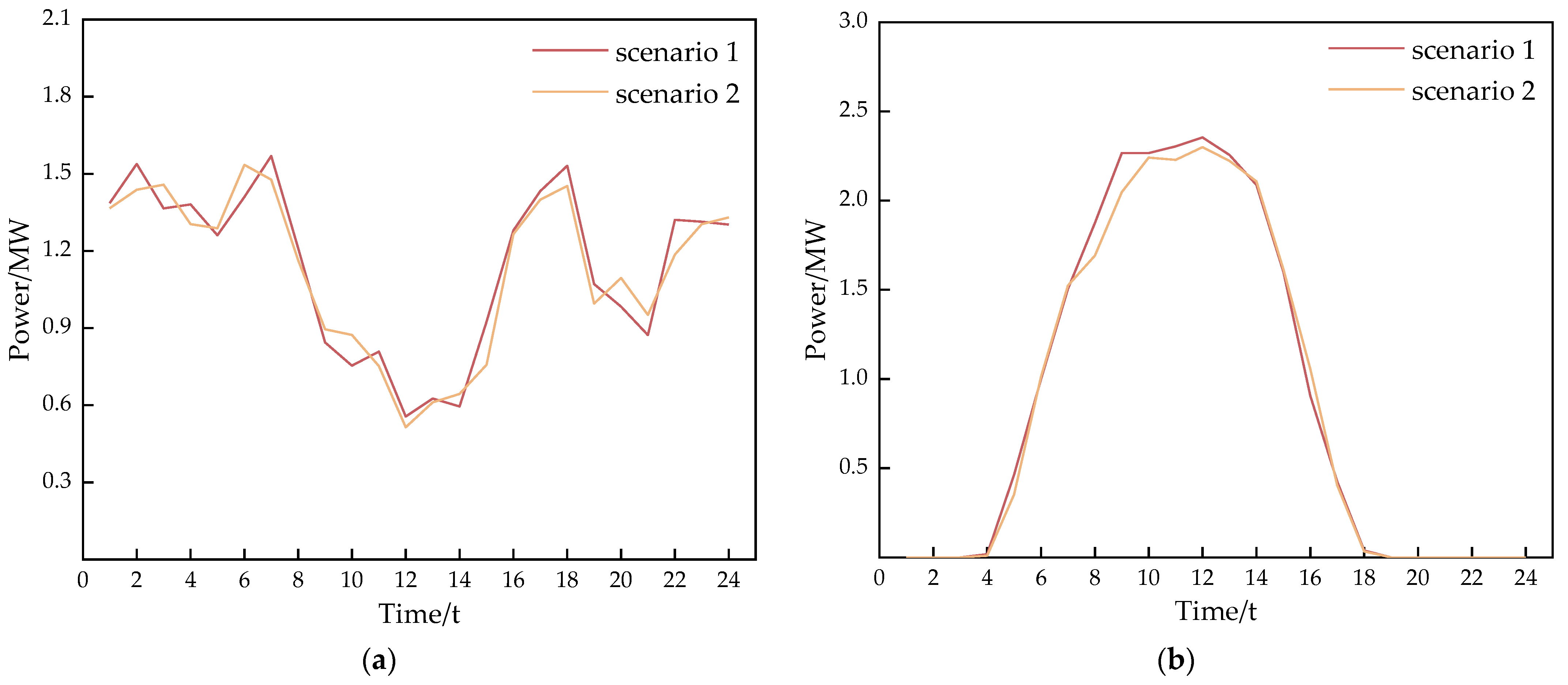
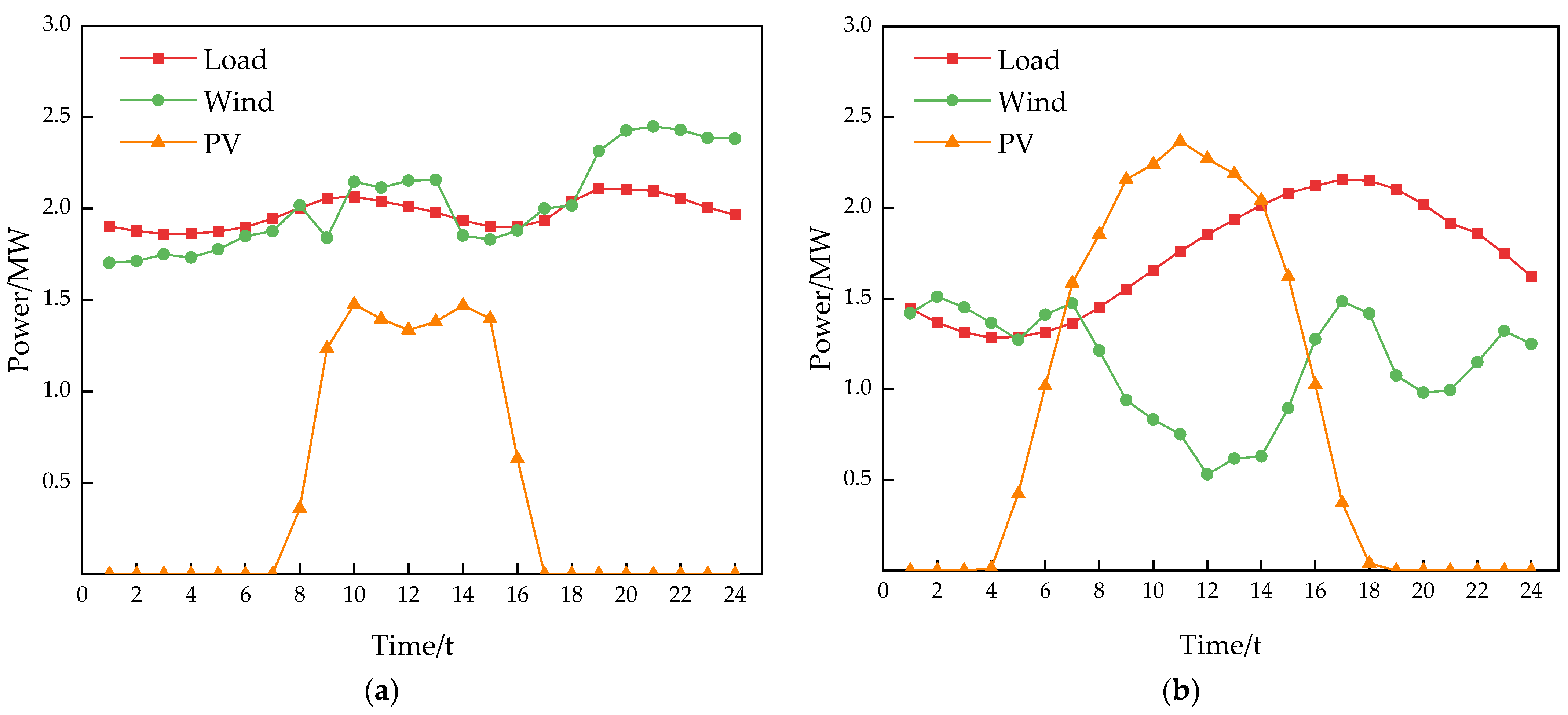
3.2. Uncertainty Handling in Wind and PV

For the uncertainty of wind power and PV, the multi-scenario method is used in this paper. It is assumed that the power of wind power and PV obeys a normal distribution. A large number of power output scenarios obeying the constraints of probability distribution are first generated using LHS sampling; then, the simultaneous backward reduction (SBR) algorithm is considered for scenario reduction.

There are various ways to realize the SBR method, and the key lies in the selection of the probability distance. The reduction of the original scene based on the Kantorovich distance can better retain the distribution characteristics of the original scene. For the generated scene set $J$, the scene with the smallest Kantorovich distance from the other scene is selected from it and placed into the scene set $J^{\prime }$. The Kantorovich distance is defined as shown below, where $s$ is the scenario for the set $J$, $s^{\prime }$ is the scenario for the set $J^{\prime }$, $d\left(s,s^{\prime }\right)$ refers to Euclidean geometric distance between $s$ and $s^{\prime }$, $\omega \left(s,s^{\prime }\right)$ stands for probability product between $s$ and $s^{\prime }$, ${\pi }_s$ is the probability that $s$ corresponds in set $J$, and ${\pi }_{s^{\prime }}$ is the probability that $s^{\prime }$ corresponds in set $J^{\prime }$.

$$\begin{array}{c}D\left(J,J^{\prime }\right)=\min \left\{{\displaystyle \sum _{s\in J,s^{\prime }\in J^{\prime }}d\left(s,s^{\prime }\right)\omega \left(s,s^{\prime }\right)}\right\}\\ {\displaystyle \sum _{s^{\prime }\in J^{\prime }}\omega \left(s,s^{\prime }\right)={\pi }_s},\forall s\in J\\ {\displaystyle \sum _{s\in J}\omega \left(s,s^{\prime }\right)={\pi }_{s^{\prime }}},\forall s^{\prime }\in J^{\prime }\\ \omega \left(s,s^{\prime }\right)\ge 0,\forall s\in J,\forall s^{\prime }\in J^{\prime }\end{array}$$

(17)

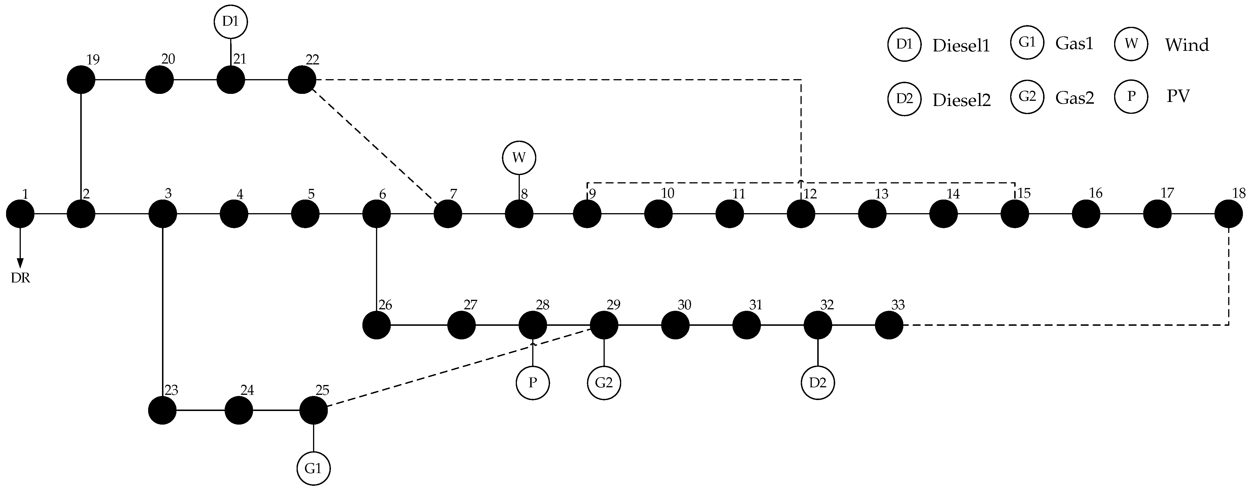
3.3. Lower Distribution Network Operation Model

3.3.1. Lower-Level Objective Function

The main costs of operating the lower distribution grid include the gas turbine generation cost $C_{gas}$, diesel unit generation cost $C_{diesel}$, wind and PV grid connection costs $C_{wind}$ and $C_{pv}$, wind and PV curtailment costs $C_{windcut}$ and $C_{pvcut}$, demand response (DR) cost $C_{DR}$, power purchase and sale costs $C_{buy}$ and $C_{sell}$, and carbon emission cost $C_{c{o}_2}$.

$$\min f_{lower}=C_{gas}+C_{diesel}+C_{pv}+C_{wind}+C_{pvcut}+C_{windcut}+C_{DR}+C_{buy}+C_{sell}+C_{c{o}_2}$$

(18)

(1)

Gas turbine generation cost

$$C_{gas}={\displaystyle \sum _{t=1}^T{\displaystyle \sum _{x=1}^M{\displaystyle \sum _{s=1}^J{\pi }_s}}}{c}_{t,x,s}^{gas}{P}_{t,x,s}^{gas}$$

(19)

where $M$ is the set of distribution network nodes, $c_{t,x,s}^{gas}$ represents unit price of gas turbine output, and $P_{t,x,s}^{gas}$ refers to the output of gas turbine.

(2)

Diesel unit generation cost

$$C_{diesel}={\displaystyle \sum _{t=1}^T{\displaystyle \sum _{x=1}^M{\displaystyle \sum _{s=1}^J{\pi }_s}}}{c}_{t,x,s}^{diesel}{P}_{t,x,s}^{diesel}$$

(20)

where $c_{t,x,s}^{diesel}$ is unit price of diesel unit output and $P_{t,x,s}^{diesel}$ refers to the output of diesel unit.

(3)

Wind and PV grid connection costs

$$C_{wind}={\displaystyle \sum _{t=1}^T{\displaystyle \sum _{x=1}^M{\displaystyle \sum _{s=1}^J{\pi }_s}}}{c}_{t,x,s}^{wind}{P}_{t,x,s}^{wind}$$

(21)

$$C_{pv}={\displaystyle \sum _{t=1}^T{\displaystyle \sum _{x=1}^M{\displaystyle \sum _{s=1}^J{\pi }_s}}}{c}_{t,x,s}^{pv}{P}_{t,x,s}^{pv}$$

(22)

where $c_{t,x,s}^{wind}$ stands for grid-connected unit price of wind power, $P_{t,x,s}^{wind}$ is the output of wind power, $c_{t,x,s}^{pv}$ stands for grid-connected unit price of PV, and $P_{t,x,s}^{pv}$ is the output of PV.

(4)

Wind and PV curtailment costs

$$C_{windcut}={\displaystyle \sum _{t=1}^T{\displaystyle \sum _{x=1}^M{\displaystyle \sum _{s=1}^J{\pi }_s}}}{c}_{t,x,s}^{wind,cut}{P}_{t,x,s}^{wind,cut}$$

(23)

$$C_{pvcut}={\displaystyle \sum _{t=1}^T{\displaystyle \sum _{x=1}^M{\displaystyle \sum _{s=1}^J{\pi }_s}}}{c}_{t,x,s}^{pv,cut}{P}_{t,x,s}^{pv,cut}$$

(24)

$$P_{t,x,s}^{wind,cut}={\sigma }_{t,x,s}^{wind,pre}{P}_{t,x,s}^{wind,pre}-P_{t,x,s}^{wind}$$

(25)

$$P_{t,x,s}^{pv,cut}={\sigma }_{t,x,s}^{pv,pre}{P}_{t,x,s}^{pv,pre}-P_{t,x,s}^{pv}$$

(26)

where $c_{t,x,s}^{wind,cut}$ represents unit price of wind curtailment, $P_{t,x,s}^{wind,cut}$ is wind curtailment, $c_{t,x,s}^{pv,cut}$ represents unit price of PV curtailment, $P_{t,x,s}^{pv,cut}$ is PV curtailment, $P_{t,x,s}^{wind,pre}$ is forecasted wind power output, $P_{t,x,s}^{pv,pre}$ is predicted output of photovoltaic, ${\sigma }_{t,x,s}^{wind,pre}$ represents wind power output prediction error parameter, and ${\sigma }_{t,x,s}^{pv,pre}$ represents PV output prediction error parameter.

(5)

DR cost

$$C_{DR}=C_{load}^{cut}+C_{load}^{trans}$$

(27)

$$C_{load}^{cut}={\displaystyle \sum _{t=1}^T{\displaystyle \sum _{x=1}^M{\displaystyle \sum _{s=1}^J{\pi }_s}}}{c}_{t,x,s}^{l,cut}{P}_{t,x,s}^{l,cut}$$

(28)

$$C_{load}^{trans}={\displaystyle \sum _{t=1}^T{\displaystyle \sum _{x=1}^M{\displaystyle \sum _{s=1}^J{\pi }_s}}}\left(c_{t,x,s}^{l,tsup}{\delta }_{t,x,s}^{l,tsup}{P}_{t,x,s}^{l,tsup}+c_{t,x,s}^{l,tsdown}{\delta }_{t,x,s}^{l,tsdown}{P}_{t,x,s}^{l,tsdown}\right)$$

(29)

where $c_{t,x,s}^{l,cut}$ stands for unit price of load shedding, $P_{t,x,s}^{l,cut}$ is load shedding, $c_{t,x,s}^{l,tsup}$ and $c_{t,x,s}^{l,tsdown}$ are unit price of transferable loads, $P_{t,x,s}^{l,tsup}$ and $P_{t,x,s}^{l,tsdown}$ are transferable loads, ${\delta }_{t,x,s}^{l,tsup}=1$ and ${\delta }_{t,x,s}^{l,tsdown}=1$ indicate transferable loads can be transferred, and ${\delta }_{t,x,s}^{l,tsup}=0$ and ${\delta }_{t,x,s}^{l,tsdown}=0$ indicate transferable loads cannot be transferred.

(6)

Power purchase and sale costs

$$C_{buy}={\displaystyle \sum _{t=1}^T{\displaystyle \sum _{x=1}^M{\displaystyle \sum _{s=1}^J{\pi }_s}}}{c}_{t,x,s}^{buy}{P}_{t,x,s}^{buy}$$

(30)

$$C_{sell}=-{\displaystyle \sum _{t=1}^T{\displaystyle \sum _{x=1}^M{\displaystyle \sum _{s=1}^J{\pi }_s}}}{c}_{t,x,s}^{sell}{P}_{t,x,s}^{sell}$$

(31)

where $c_{t,x,s}^{buy}$ is unit price of electricity purchased, $P_{t,x,s}^{buy}$ is amount of electricity purchased, $c_{t,x,s}^{sell}$ represents unit price of electricity sold, and $P_{t,x,s}^{sell}$ represents amount of electricity sold.

(7)

Carbon emission cost

$$C_{c{o}_2}={\displaystyle \sum _{t=1}^T{\displaystyle \sum _{x=1}^M{\displaystyle \sum _{s=1}^J{\pi }_s}}}{c}_{t,x,s}^E\left[\left(E_{t,x,s}^{gas}-A_{t,x,s}^{gas}\right)+\left(E_{t,x,s}^{diesel}-A_{t,x,s}^{diesel}\right)+\left(E_{t,x,s}^{buy}-A_{t,x,s}^{buy}\right)\right]$$

(32)

$$E_{t,x,s}^{gas}=e_{t,x,s}^{gas}{P}_{t,x,s}^{gas}$$

(33)

$$A_{t,x,s}^{gas}=q_{t,x,s}^{gas}{P}_{t,x,s}^{gas}$$

(34)

$$E_{t,x,s}^{diesel}=e_{t,x,s}^{diesel}{P}_{t,x,s}^{diesel}$$

(35)

$$A_{t,x,s}^{diesel}=q_{t,x,s}^{diesel}{P}_{t,x,s}^{diesel}$$

(36)

$$E_{t,x,s}^{buy}=e_{t,x,s}^{buy}{P}_{t,x,s}^{buy}$$

(37)

$$A_{t,x,s}^{buy}=q_{t,x,s}^{buy}{P}_{t,x,s}^{buy}$$

(38)

where $c_{t,x,s}^E$ is carbon emission base price, $E_{t,x,s}^{gas}$ stands for gas turbine carbon emissions, $A_{t,x,s}^{gas}$ stands for gas turbine carbon allowances, $E_{t,x,s}^{diesel}$ represents carbon emissions from diesel unit, $A_{t,x,s}^{diesel}$ represents carbon allowances from diesel unit, $E_{t,x,s}^{buy}$ refers to carbon emissions from purchased electricity, $A_{t,x,s}^{buy}$ refers to carbon allowances from purchased electricity, $e_{t,x,s}^{gas}$ is gas turbine carbon emission coefficient, $e_{t,x,s}^{diesel}$ is diesel unit carbon emission coefficient, $e_{t,x,s}^{buy}$ is carbon emission coefficient for purchased electricity, $q_{t,x,s}^{gas}$ represents gas turbine carbon allowance coefficient, $q_{t,x,s}^{diesel}$ represents diesel unit carbon allowance coefficient, and $q_{t,x,s}^{buy}$ represents electricity purchase carbon allowance coefficient.

3.3.2. Lower-Level Constraints

(1)

Gas turbine output constraint

$$0\le P_{t,x,s}^{gas}\le P_{t,x,s,\max }^{gas}$$

(39)

where $P_{t,x,s,\max }^{gas}$ is maximum gas turbine output.

(2)

Gas turbine climb constraint

$$P_{t,x,s,\min }^{gas,ramp}\le P_{t,x,s}^{gas}-P_{t-1,x,s}^{gas}\le P_{t,x,s,\max }^{gas,ramp}$$

(40)

where $P_{t,x,s,\min }^{gas,ramp}$ represents minimum climbing output of gas turbine and $P_{t,x,s,\max }^{gas,ramp}$ represents maximum climbing output of gas turbine.

(3)

Diesel unit output constraint

$$0\le P_{t,x,s}^{diesel}\le P_{t,x,s,\max }^{diesel}$$

(41)

where, $P_{t,x,s,\max }^{diesel}$ refers to maximum gas turbine output.

(4)

Diesel unit climb constraint

$$P_{t,x,s,\min }^{diesel,ramp}\le P_{t,x,s}^{diesel}-P_{t-1,x,s}^{diesel}\le P_{t,x,s,\max }^{diesel,ramp}$$

(42)

where $P_{t,x,s,\min }^{diesel,ramp}$ stands for minimum climbing output of gas turbine and $P_{t,x,s,\max }^{diesel,ramp}$ stands for maximum climbing output of gas turbine.

(5)

Wind and photovoltaic output constraints

$$0\le P_{t,x,s}^{wind}\le {\sigma }_{t,x,s}^{wind,pre}{P}_{t,x,s}^{wind,pre}$$

(43)

$$0\le P_{t,x,s}^{pv}\le {\sigma }_{t,x,s}^{pv,pre}{P}_{t,x,s}^{pv,pre}$$

(44)

(6)

Power purchase and sale constraints

$$0\le P_{t,x,s}^{buy}\le P_{t,x,s,\max }^{buy}$$

(45)

$$0\le P_{t,x,s}^{sell}\le P_{t,x,s,\max }^{sell}$$

(46)

where $P_{t,x,s,\max }^{buy}$ refers to upper limit of purchased power and $P_{t,x,s,\max }^{sell}$ refers to upper limit of electricity sales.

(7)

DR constraints

$$0\le P_{t,i,s}^{l,cut}\le {\varsigma }_{t,i,s}^{l,cut}{P}_{t,i,s}^{l,pre}$$

(47)

$$0\le P_{t,i,s}^{l,tsup}\le {\delta }_{t,i,s}^{l,tsup}{\varsigma }_{t,i,s}^{l,tsup}{P}_{t,i,s}^{l,pre}$$

(48)

$$0\le P_{t,i,s}^{l,tsdown}\le {\delta }_{t,i,s}^{l,tsdown}{\varsigma }_{t,i,s}^{l,tsdown}{P}_{t,i,s}^{l,pre}$$

(49)

$${\delta }_{t,i,s}^{l,tsup}+{\delta }_{t,i,s}^{l,tsdown}\le 1$$

(50)

$${\displaystyle \sum _{t=1}^T{\displaystyle \sum _{x=1}^M{\displaystyle \sum _{s=1}^J{\pi }_s{P}_{t,x,s}^{l,tsup}}}}={\displaystyle \sum _{t=1}^T{\displaystyle \sum _{x=1}^M{\displaystyle \sum _{s=1}^J{\pi }_s{P}_{t,x,s}^{l,tsdown}}}}$$

(51)

where ${\varsigma }_{t,i,s}^{l,cut}$ is load shedding coefficient, and ${\varsigma }_{t,i,s}^{l,tsup}$ and ${\varsigma }_{t,i,s}^{l,tsdown}$ are transferable load coefficients.

(8)

Distribution network power flow constraints

$$P_{t,x,s}^{xnz}+{\displaystyle \sum _{z<x}{P}_{t,zx,s}}=P_{t,x,s}^{load}+{\displaystyle \sum _{v>x}{P}_{t,xv,s}}$$

(52)

$$Q_{t,x,s}^{xnz}+{\displaystyle \sum _{z<x}{Q}_{t,zx,s}}=Q_{t,x,s}^{load}+{\displaystyle \sum _{v>x}{Q}_{t,xv,s}}$$

(53)

$$U_{t,x,s}^2-U_{t,z,s}^2=2\left(r_{xz}{P}_{t,xz,s}+x_{xz}{Q}_{t,xz,s}\right)$$

(54)

$${\left(U_x^{\min }\right)}^2\le U_{t,x,s}^2\le {\left(U_x^{\max }\right)}^2$$

(55)

$$-S_l\le P_{t,xz,s}^{xnz}\le S_l$$

(56)

$$-S_l\le Q_{t,xz,s}^{xnz}\le S_l$$

(57)

$$-\sqrt{2}{S}_l\le P_{t,xz,s}^{xnz}+Q_{t,xz,s}^{xnz}\le \sqrt{2}{S}_l$$

(58)

$$-\sqrt{2}{S}_l\le P_{t,xz,s}^{xnz}-Q_{t,xz,s}^{xnz}\le \sqrt{2}{S}_l$$

(59)

where $P_{t,x,s}^{xnz}$ is injected power; $P_{t,x,s}^{load}$ is load power; ${\displaystyle \sum _{z<x}{P}_{t,zx,s}}$ refers to the sum of branch active power injected into node $x$; ${\displaystyle \sum _{v>x}{P}_{t,xv,s}}$ refers to the sum of branch active power flowing out of node $x$; and $Q_{t,x,s}^{xnz}$, $Q_{t,x,s}^{load}$, ${\displaystyle \sum _{z<x}{Q}_{t,zx,s}}$, and ${\displaystyle \sum _{v>x}{Q}_{t,xv,s}}$ have the same meaning. $P_{t,xz,s}^{xnz}$ and $Q_{t,xz,s}^{xnz}$ are active and reactive power flowing in line $xz$, $U_x^{\min }$ represents minimum value of node voltage, $U_x^{\max }$ represents maximum value of node voltage, $r_{xz}$ stands for resistance on line $xz$, and $x_{xz}$ stands for reactance on line $xz$. $S_l$ is line capacity.

(9)

Power balance constraint

$$\begin{array}{l}{P}_{t,x,s}^{gas}+P_{t,x,s}^{diesel}+P_{t,x,s}^{wind}+P_{t,x,s}^{pv}+P_{t,x,s}^{buy}+P_{t,x,s}^{l,cut}+P_{t,x,s}^{l,tsup}+{\displaystyle \sum _{z<x}{P}_{t,zx,s}}=\\ P_{t,x,s}^{sell}+P_{t,x,s}^{l,car}+P_{t,x,s}^{l,pre}+P_{t,x,s}^{l,tsdown}+{\displaystyle \sum _{v>x}{P}_{t,xv,s}}\end{array}$$

(60)

$$Q_{t,x,s}^{gas}+Q_{t,x,s}^{diesel}+Q_{t,x,s}^{l,cut}+Q_{t,x,s}^{l,tsup}+{\displaystyle \sum _{z<x}{Q}_{t,zx,s}}=Q_{t,x,s}^{l,pre}+Q_{t,x,s}^{l,tsdown}+{\displaystyle \sum _{v>x}{Q}_{t,xv,s}}$$

(61)

where $P_{t,x,s}^{l,car}$ is EV charging load.

4. KKT Conditions for Solving the Bi-Level Model

For bi-level optimization problems, a common solution is to replace the lower-level problem with the KKT conditions of the lower-level problem. The KKT conditions formed by the lower-layer model are as follows:

$$\left\{\begin{array}{l}L=f_{lower}+\lambda H_{cons}+\mu G_{cons}\hfill \\ H_{cons}=0\hfill \\ G_{cons}\le 0\hfill \\ \lambda ,\mu \ge 0\hfill \end{array}\right.$$

(62)

where $f_{lower}$ is the objective function of the lower level problem, $H_{cons}$ is equation constraints for lower level problems, $G_{cons}$ is inequality constraints for lower level problems, and $\lambda$ and $\mu$ represent Lagrange multipliers.

The Lagrangian function for the lower-level optimization problem in this paper is constructed as shown below. In order to simplify the functional equation, a gas turbine is used as an example to construct according to the format of Equation (62).

Firstly, convert Equations (33), (34), and (60) to the form of $H_{cons}=0$. The transformed forms are shown in Equations (63)–(65).

$$E_{t,x,s}^{gas}-e_{t,x,s}^{gas}{P}_{t,x,s}^{gas}=0$$

(63)

$$A_{t,x,s}^{gas}-q_{t,x,s}^{gas}{P}_{t,x,s}^{gas}=0$$

(64)

$$\begin{array}{l}{P}_{t,x,s}^{gas}+P_{t,x,s}^{diesel}+P_{t,x,s}^{wind}+P_{t,x,s}^{pv}+P_{t,x,s}^{buy}+P_{t,x,s}^{l,cut}+P_{t,x,s}^{l,tsup}+{\displaystyle \sum _{z<x}{P}_{t,zx,s}}-\\ P_{t,x,s}^{sell}-P_{t,x,s}^{l,car}-P_{t,x,s}^{l,pre}-P_{t,x,s}^{l,tsdown}-{\displaystyle \sum _{v>x}{P}_{t,xv,s}}=0\end{array}$$

(65)

Then, convert Equations (39) and (40) to the form of $G_{cons}\le 0$. The transformed forms are shown in Equations (66)–(69).

$$P_{t,x,s}^{gas}-P_{t,x,s,\max }^{gas}\le 0$$

(66)

$$0-P_{t,x,s}^{gas}\le 0$$

(67)

$$P_{t,x,s}^{gas}-P_{t-1,x,s}^{gas}-P_{t,x,s,\max }^{gas,ramp}\le 0$$

(68)

$$P_{t,x,s,\min }^{gas,ramp}-P_{t,x,s}^{gas}+P_{t-1,x,s}^{gas}\le 0$$

(69)

Finally, write $f_{lower}$, $H_{cons}$, and $G_{cons}$ in the form of $L=f_{lower}+\lambda H_{cons}+\mu G_{cons}$. The form is shown in Equation (70).

$$\begin{array}{l}L=f_{lower}+{\displaystyle \sum _{t=1}^T{\displaystyle \sum _{x=1}^M{\displaystyle \sum _{s=1}^J{\pi }_s\left[{\lambda }_{t,x,s}^1\left(E_{t,x,s}^{gas}-e_{t,x,s}^{gas}{P}_{t,x,s}^{gas}\right)+{\lambda }_{t,x,s}^2\left(A_{t,x,s}^{gas}-q_{t,x,s}^{gas}{P}_{t,x,s}^{gas}\right)\right.}}}\\ \left.\left.+{\lambda }_{t,x,s}^{10}\left(P_{t,x,s}^{gas}\right.+P_{t,x,s}^{diesel}+P_{t,x,s}^{wind}+P_{t,x,s}^{pv}+P_{t,x,s}^{buy}+P_{t,x,s}^{l,cut}+P_{t,x,s}^{l,tsup}\right)\right]+\overline{{\mu }_{t,x,s}^{gas}}\left(P_{t,x,s}^{gas}\right.\\ \left.-P_{t,x,s,\max }^{gas}\right)+\underset{¯}{{\mu }_{t,x,s}^{gas}}\left(0-P_{t,x,s}^{gas}\right)+\overline{{\mu }_{t,x,s}^{gas,ramp}}\left(P_{t,x,s}^{gas}-P_{t-1,x,s}^{gas}-P_{t,x,s,\max }^{gas,ramp}\right)+\underset{¯}{{\mu }_{t,x,s}^{gas,ramp}}\\ \left(P_{t,x,s,\min }^{gas,ramp}-P_{t,x,s}^{gas}+P_{t-1,x,s}^{gas}\right)+\overline{{\mu }_{t-1,x,s}^{gas,ramp}}\left(P_{t,x,s}^{gas}-P_{t-1,x,s}^{gas}-P_{t,x,s,\max }^{gas,ramp}\right)+\underset{¯}{{\mu }_{t-1,x,s}^{gas,ramp}}\\ \left(P_{t,x,s,\min }^{gas,ramp}-P_{t,x,s}^{gas}+P_{t-1,x,s}^{gas}\right)\end{array}$$

(70)

This leads to the following Lagrangian smoothness constraint for the optimization problem in this paper. The gas turbine is used as an example, and the rest are shown in Appendix A.

$$\frac{\partial L}{\partial P_{t,x,s}^{gas}}={\pi }_s{c}_{t,x,s}^{gas}-e_{t,x,s}^{gas}{\lambda }_{t,x,s}^1-q_{t,x,s}^{gas}{\lambda }_{t,x,s}^2+{\lambda }_{t,x,s}^{10}+\overline{{\mu }_{t,x,s}^{gas}}-\underset{¯}{{\mu }_{t,x,s}^{gas}}+\overline{{\mu }_{t,x,s}^{gas,ramp}}-\underset{¯}{{\mu }_{t,x,s}^{gas,ramp}}=0$$

(71)

$$\frac{\partial L}{\partial P_{t-1,x,s}^{gas}}=-\overline{{\mu }_{t-1,x,s}^{gas,ramp}}+\underset{¯}{{\mu }_{t-1,x,s}^{gas,ramp}}=0$$

(72)

where the dual variables similar to $\overline{{\mu }_{t,x,s}^{gas}}$ and $\underset{¯}{{\mu }_{t,x,s}^{gas}}$ are nonlinear and need to be linearized using the large M method. The linearization is shown as follows.

$$\begin{array}{l}0\le \overline{{\mu }_{t,x,s}^{gas}}\le M\overline{{\beta }_{t,x,s}^{gas}}\\ 0\le P_{t,x,s,\max }^{gas}-P_{t,x,s}^{gas}\le M\left(1-\overline{{\beta }_{t,x,s}^{gas}}\right)\\ 0\le \underset{¯}{{\mu }_{t,x,s}^{gas}}\le M\underset{¯}{{\beta }_{t,x,s}^{gas}}\\ 0\le P_{t,x,s}^{gas}-0\le M\left(1-\underset{¯}{{\beta }_{t,x,s}^{gas}}\right)\end{array}$$

(73)

where $\overline{{\beta }_{t,x,s}^{gas}}$ and $\underset{¯}{{\beta }_{t,x,s}^{gas}}$ are binary variables, and $M$ is an infinitely large number.

The charging station bi-level planning model is transformed into a single-level optimization model through KKT conditional equivalence. Its specific form is as follows.

$$\min f_{upper}=f_1+f_2$$

(74)

Constraints include Equations (13)–(16), Equations (52)–(61), Equations (71) and (73), and Equations (A1)–(A32).

5. Example Analysis

5.1. Parameter Setting

In order to illustrate the effectiveness of the proposed method, a city road network in the southeastern part of South Dakota, USA, is selected as the area to be planned for validation. The specific situation is shown in Figure 5. The number on the line between two points indicates the distance. According to the attributes of the city, its functional areas are divided into the populated area, the industrial zone, and the commercial area. There are a total of 6000 electric vehicles in the region, including 1800 private cars, 3000 online car-hailings, 900 morning cabs, and 300 evening cabs. The private car is powered by the BYD Yuan PLUS series with a capacity of 49.92 kWh. The online car-hailing and cabs adopt the BYD Seagull series, with a capacity of 30.08 kWh. Private vehicle trip chains are set up to a maximum length of three, all of which originate from and eventually return to residential areas. The relevant parameters in the transportation network are shown in

Table 1. The relevant parameters in the transportation network.

Parameter Symbol	Parameter Value	Parameter Symbol	Parameter Value
$C_{iv,i}$	CNY 1,000,000	$T_{day}$	12/h
$C_{fast}$	CNY 20,000	$y$	10
$C_{slow}$	CNY 5000	$r_0$	0.08
$C_{i,chp}$	CNY 0.5	$\upsilon$	0.0073
$\theta$	CNY 20	$\partial$	0.01
$P_{fast}$	0.048 CNY/MW	$N_{\max }$	24
$P_{slow}$	0.012 CNY/MW	$N_{\min }$	3

.

In this paper, an improved 33-node distribution network is used, as shown in Figure 6. The distribution grid operation time scale is chosen to be 48 h with the typical winter day and the typical summer day. Typical daily load versus wind and PV power curves are shown in Figure 7. Two scenarios are considered for wind and PV. Scenario generation and scenario reduction diagrams for wind and PV are shown in Appendix B, Figure A1, Figure A2, Figure A3 and Figure A4. Power purchase and sale prices are in the form of time-of-day tariffs, as shown in

Table 2. Purchase and sale price of electricity.

Categories	Time Interval	Price/(CNY/MWh)
Electricity purchase	Off-peak time (22:00~7:00)	500
	Shoulder time (7:00~11:00, 14:00~18:00)	750
	Peak time (11:00~14:00, 18:00~22:00)	1200
Electricity sale	Whole day	300

. The relevant parameters of the gas turbine and diesel unit are in

Table 3. Parameters of the gas turbine and diesel unit.

Unit Number	Upper and Lower Limits of Output	Climbing Upper and Lower Limits
Gas turbine 1	0.8/MW	0.4/MW
Gas turbine 2	0.8/MW	0.4/MW
Diesel unit 1	1.2/MW	0.4/MW
Diesel unit 2	1.2/MW	0.4/MW

. The remaining relevant parameters in the distribution network are shown in

Table 4. The remaining relevant parameters in the distribution network.

Parameter Symbol	Parameter Value	Parameter Symbol	Parameter Value
$c_{t,x,s}^{gas}$	CNY 413	$c_{t,x,s}^E$	375/(CNY/t)
$c_{t,x,s}^{diesel}$	CNY 490	$e_{t,x,s}^{gas}$	0.4035/(t/MW)
$c_{t,x,s}^{wind}$	CNY 650	$e_{t,x,s}^{diesel}$	0.6583/(t/MW)
$c_{t,x,s}^{pv}$	CNY 650	$e_{t,x,s}^{buy}$	1.72/(t/MW)
$c_{t,x,s}^{wind,cut}$	CNY 300	$q_{t,x,s}^{gas}$	0.3901/(t/MW)
$c_{t,x,s}^{pv,cut}$	CNY 300	$q_{t,x,s}^{diesel}$	0.4828/(t/MW)
$c_{t,x,s}^{l,cut}$	CNY 100	$q_{t,x,s}^{buy}$	0.8729/(t/MW)
$c_{t,x,s}^{l,tsup}$	CNY 100	${\varsigma }_{t,i,s}^{l,cut}$	0.05
$c_{t,x,s}^{l,tsdown}$	CNY 100	${\varsigma }_{t,i,s}^{l,tsup}$	0.1
$c_{t,x,s}^{sell}$	CNY 300	${\varsigma }_{t,i,s}^{l,tsdown}$	0.1

.

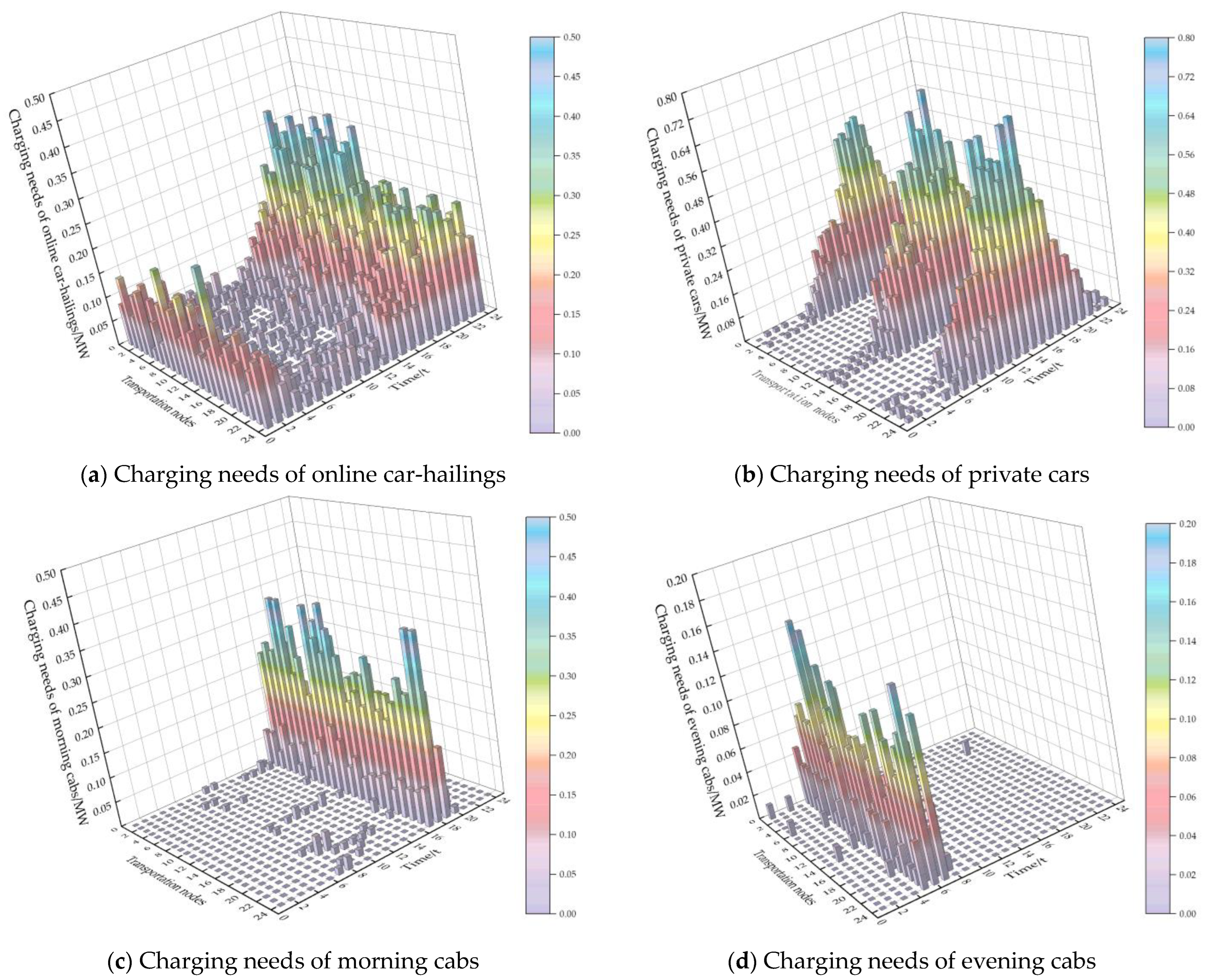
5.2. Charging Demand Load Forecast Results

Based on the EV charging load prediction model proposed in Section 2 of this paper, the spatial and temporal distribution of EV charging load in a day is obtained as shown in Figure 8. Figure 8a shows the charging load demand distribution of online car-hailings. Online car-hailings start around 7:00 a.m. and finish around 10 p.m. Since the driving condition of online car-hailings in a day is related to the customer’s demand, the distribution of its charging load on the nodes of the transportation network has a large randomness, and the peak charging time is concentrated at 18:00~24:00 h. Figure 8b shows the charging load demand distribution for private vehicles. According to the private car travel chain, it can be seen that private cars leave from residential areas at around 7:00 a.m. and return to residential areas at around 17:00 p.m., and in the middle of the 7:00 to 17:00 p.m. period they may go to an industrial area, a commercial area, or both. Therefore, the charging load of private cars is more regularly distributed in the nodes of the transportation network, with most of them located in the nodes where residential areas are located, and very few in the nodes where commercial or industrial areas are located. The peak charging time is mainly concentrated in the period of 13:00 to 18:00 h. Figure 8c shows the distribution of charging load demand for morning cabs. Early morning cabs have a relatively fixed commuting time, going to work at 7:00 a.m. and leaving work at 17:00 p.m. Their driving conditions in a day are similar to those of online car-hailings, so the distribution of the charging load in the nodes of the transportation network also has a large degree of randomness, and the peak charging time period is from 17:00 to 19:00. The situation of evening cabs is similar to that of morning cabs, whose peak charging time period is from 5:00 to 7:00 p.m. Combining the above EV charging load distribution in time with the peak and valley load periods of the distribution network, it can be seen that the total load becomes more in the peak period, and the load difference in the peak and valley periods is bigger, which brings more challenges to the operation of the distribution network.

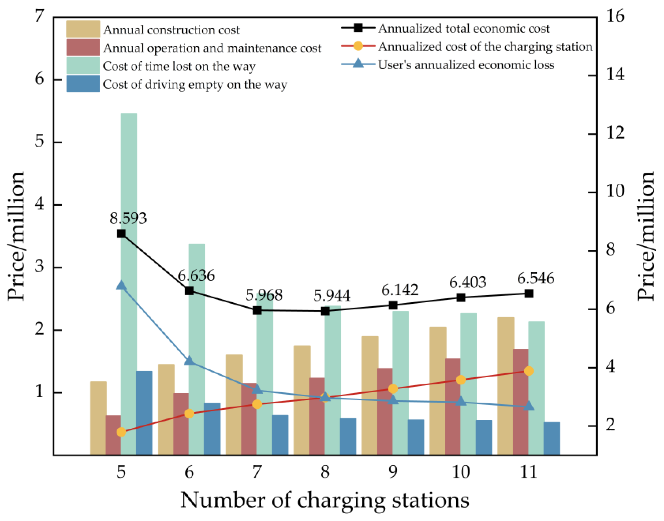
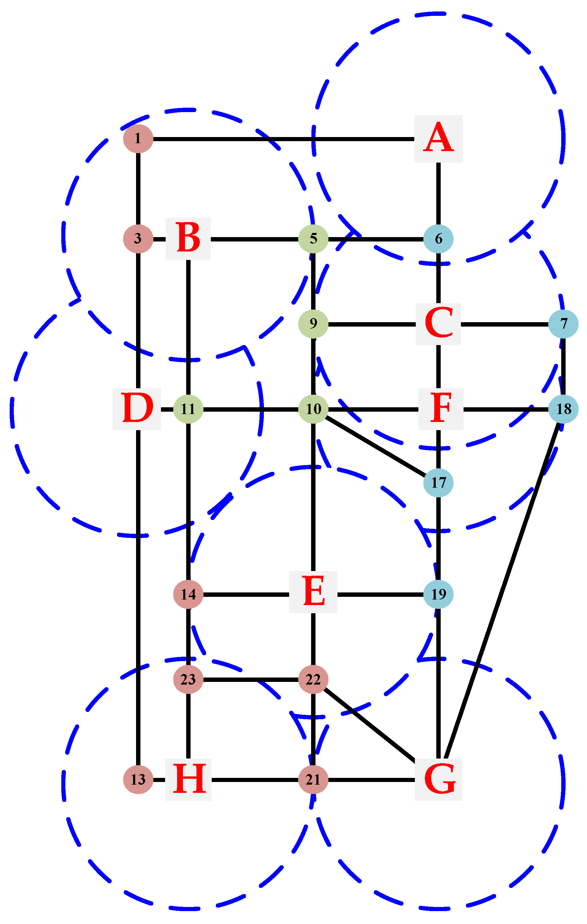
5.3. Results of Charging Station Siting and Capacity Determination

On the basis of obtaining the spatial and temporal distribution of EV charging demand load, a two-layer optimization model is constructed to site and set the capacity of charging stations. The comprehensive optimization results with the objective of minimizing the cost of the charging station and user loss are shown in

Table 5. Costs in the siting and capacity of charging stations.

Number of Charging Stations	Annualized Cost of the Charging Station/Million	User’s Annualized Economic Loss/Million	Annualized Total Economic Cost/Million
5	1.797	6.795	8.593
6	2.431	4.205	6.636
7	2.747	3.221	5.968
8	2.975	2.969	5.944
9	3.278	2.863	6.142
10	3.582	2.821	6.403
11	3.888	2.658	6.546

and Figure 9.

In this paper, the number of charging stations is set from 3 to 24, and the charging service radius is 2.5 km. Charging station cost minimization and user loss minimization are contradictory. The smaller the cost of the charging station, the smaller the number of charging stations built, the EV users’ charging needs for charging nearby cannot be met, and the greater the user’s loss. Conversely, the smaller the user’s loss, the more charging stations will be built and the greater the resulting charging station cost will be. Table 5 and Figure 9 show the cost comparison of various types of charging station building stations from five to eleven seats. When there are only five charging stations, the charging range does not cover the whole area. Vehicles in some nodes need to travel a long distance to charge. The resulting cost of time lost on the way and cost of driving empty on the way is huge, and its value even far exceeds the annual construction cost and the annual operation and maintenance cost. When the number of charging stations is gradually increased and the charging range is sufficient to cover the whole area, even with some overlapping, most of the EV users can choose the nearest charging station for charging; thus, the cost of time lost on the way and cost of driving empty on the way are greatly reduced. However, the increase in the number of charging stations also leads to an increase in the annual construction cost and the annual operation and maintenance cost.

The optimal number of stations optimized by the model in this paper is eight, and its combined cost of charging station cost and user loss minimization is 5.944 million. These eight charging stations cover all nodes in the urban area that require charging and minimize the overlap of charging service areas. Avoid wastage of maintenance and warranty costs due to idle charging stations. Let the eight charging stations be numbered as A, B, C, D, E, F, G, and H. The planning layout of urban charging stations is shown in Figure 10.

On the basis of determining the optimal location of the charging stations, the total number of charging piles in each charging station is determined in this paper based on the daily charging demand of EV users at each node of the transportation network. The results are shown in

Table 6. Location of charging station installations and total number of charging piles at each charging station.

Charging Station Number	Transportation Network Nodes	Corresponding Distribution Nodes	Total Number of Charging Piles
A	2	6	18
B	4	2	42
C	8	7	37
D	12	30	24
E	15	10	48
F	16	9	42
G	20	14	20
H	24	18	62

. In addition, this paper determines the specific number of fast-charging piles and slow-charging piles in each charging station according to the divided urban functional areas. The results are shown in Figure 11.

Based on the EV charging demand load forecasting model in Section 2, it is observed that the daily charging demand is higher in nodes 4, 8, 15, 16, and 24 of the transportation network while the daily charging demand is comparatively smaller in nodes 2, 12, and 20. Therefore, the total number of charging piles installed in charging stations B, C, E, F, and H is higher and the total number of charging piles installed in charging stations A, D, and G is lower.

As can be seen in Figure 11, the number of fast-charging piles at Charging Station B is much larger than the number of slow-charging piles. This is because the area where charging station B is located is a commercial area, and EV users usually do not stay for a long time in the commercial area. The charging power and charging time of slow chargers cannot meet the charging demand of users in such areas. Therefore, the number of fast-charging piles will be larger. The number of slow-charging piles is slightly larger than the number of fast-charging piles at charging station F. This is because the area where charging station F is located is an industrial area, and EV users usually stay in the industrial area from working hours to off-duty hours, so there is enough time for charging through the slow-charging piles. The fast-charging piles are set up to cater for users who are not always in the office. The area where charging station G and charging station H are located is a residential area, and the number of fast-charging piles and the number of slow-charging piles in the station are basically equal. Users in residential areas usually install home charging piles according to their own needs, with the slow-charging piles being used for charging when they are at home for a long time and the fast-charging piles being used for charging when they go out in an emergency.

5.4. Distribution Network Operating Results

The study of charging station siting and capacity should not only consider whether to meet the demand of EV charging load but also whether the distribution network can operate properly after connecting to the charging station. Nowadays, wind and PV curtailment rate and carbon emissions have been the focus of research in distribution grid operation.

Table 7. Comparison of carbon emissions, and wind and PV curtailment, before and after charging stations are connected to the distribution grid.

Distribution Network Scenarios	Wind Curtailment Rate		PV Curtailment Rate		Carbon Emission/t	Carbon Emission Penalty/CNY
Not consider charging station access	Winter	8.72%	Winter	81.10%	2.85	1067.66
	Summer	22.82%	Summer	66.48%
Consider charging station access	Winter	−0.48%	Winter	42.48%	4.03	1510.77
	Summer	13.74%	Summer	16.99%

shows the wind and PV curtailment rate and carbon emission in the improved 33-node distribution network before and after connecting the charging station.

Typical winter days have more wind energy and less solar energy. When the distribution grid is dispatched and operated, wind energy is mainly utilized in conjunction with gas turbines and diesel units to balance the load demand on a typical winter day and solar energy is less utilized. Conversely, typical summer days have more solar and less wind. When the distribution grid is dispatched, solar energy is primarily utilized in conjunction with diesel and gas turbines to balance typical summer day load demands and wind energy is utilized at a lower rate.

In the bi-level optimization model proposed in this paper, comparing the distribution grid access to the charging station before and after, it can be found that the wind curtailment rate decreases by 9.2% and the PV curtailment rate decreases by 38.62% on a typical day in winter. Moreover, the wind curtailment rate decreases by 9.08% and the PV curtailment rate decreases by 49.49% on a typical day in summer. Due to the access of charging stations, more loads become available in the distribution network. The output of gas turbines and diesel units, which contain carbon emissions, increased. As a result, the overall carbon emissions of the distribution network increased by 1.18 t and the carbon penalty fee increased by CNY 443.11.

Through the above analysis, the model proposed in this paper can effectively reduce the wind and PV curtailment rate with a small increase in carbon emissions.

6. Conclusions

In this paper, for the problem of EV charging station siting and capacity determination, on the one hand, the driving status of online car-hailings and cabs is determined by OD matrix and Dijkstra’s shortest path algorithm; on the other hand, the driving status of private cars is determined by travel chain model and then combined with the LHS method to obtain the charging demand of each type of vehicle based on the transportation nodes’ charging demand. Based on this, a bi-level planning model for charging stations is proposed by combining the distribution network operation model with the spatial and temporal distribution characteristics of the charging demand. The KKT condition is used to transform the bi-level model into a single-level model to solve and obtain the charging station location and capacity. The conclusions obtained through the analysis of examples are as follows:

(1)

The spatial and temporal distribution of charging load demand in the transportation road network is related to the division of urban functional areas and the charging characteristics of the functional areas, such as the high charging load demand and long charging time in residential areas in general. The validity of the EV charging load prediction model is verified.

(2)

By comprehensively considering the interests of both users’ losses and charging station costs, the bi-level planning model is solved to obtain the optimal number of charging stations and the optimal number of charging piles to be included in each charging station, and the number of fast-charging piles and the number of slow-charging piles are subdivided according to the functional areas of the city, which is consistent with the actual demand and can be used for the charging station planning in the city.

(3)

By analyzing and comparing the effects on the overall carbon emissions, and wind and PV curtailment rate, in the distribution network operation before and after access to the charging station, it is found that access to the charging station increases carbon emissions by a small amount; however, at the same time, it can greatly reduce the wind and PV curtailment rate, which verifies the correctness of the bi-level planning model.

References

1. Das, H.; Rahman, M.; Li, S.; Tan, C. Electric vehicles standards, charging infrastructure, and impact on grid integration: A technological review. Renew. Sustain. Energy Rev. 2020, 120, 109618. [Google Scholar] [CrossRef]
2. Hu, Z.; Liu, S.; Luo, W. Intrusion-detector-dependent distributed economic model predictive control for load frequency regulation with PEVs under cyber attacks. IEEE Trans. Circuits Syst. I Regul. Pap. 2021, 68, 3857–3868. [Google Scholar] [CrossRef]
3. Huang, Z.; Fang, B.; Deng, J. Multi-objective optimization strategy for distribution network considering V2G-enabled electric vehicles in building integrated energy system. Prot. Control Mod. Power Syst. 2020, 5, 48–55. [Google Scholar] [CrossRef]
4. Zhang, Y.; Zhang, Q.; Farnoosh, A.; Chen, S.; Li, Y. GIS-based multi-objective particle swarm optimization of charging stations for electric vehicles. Energy 2019, 169, 844–853. [Google Scholar] [CrossRef]
5. Wang, C.; Ju, P.; Wu, F.; Pan, X.; Wang, Z. A systematic review on power system resilience from the perspective of generation, network, and load. Renew. Sustain. Energy Rev. 2022, 167, 112567. [Google Scholar] [CrossRef]
6. Mazumder, S.; Voss, L.; Dowling, K.; Conway, A.; Hall, D. Overview of wide/ultrawide bandgap power semiconductor devices for distributed energy resources. IEEE J. Emerg. Sel. Top. Power Electron. 2023, 11, 3957–3982. [Google Scholar] [CrossRef]
7. Sun, J.; Xu, J.; Ke, D.; Liao, S.; Ling, Z. Cluster partition for distributed energy resources in regional integrated energy system. Energy Rep. 2023, 9, 613–619. [Google Scholar] [CrossRef]
8. Strezoski, L.; Simic, N. Quantifying the impact of inverter-based distributed energy resource modeling on calculated fault current flow in microgrids. Int. J. Electr. Power Energy Syst. 2023, 151, 109161. [Google Scholar] [CrossRef]
9. Wang, C.; Lei, S.; Ju, P.; Chen, C.; Peng, C.; Hou, Y. MDP-based distribution network reconfiguration with renewable distributed generation: An approximate dynamic programming approach. IEEE Trans. Smart Grid 2020, 11, 3620–3631. [Google Scholar] [CrossRef]
10. Wang, C.; Ju, P.; Lei, S.; Wang, Z.; Wu, F.; Hou, Y. Markov decision process-based resilience enhancement for distribution systems: An approximate dynamic programming approach. IEEE Trans. Smart Grid 2020, 11, 2498–2510. [Google Scholar] [CrossRef]
11. Hamrahi, M.; Mallaki, M.; Pirkolachahi, N.; Shirazi, N. Flexibility pricing of grid-connected energy hubs in the presence of uncertain energy resources. Int. J. Energy Res. 2023, 2023, 6798904. [Google Scholar] [CrossRef]
12. Wu, C.; Jiang, S.; Gao, S.; Liu, Y.; Han, H. Charging demand forecasting of electric vehicles considering uncertainties in a microgrid. Energy 2022, 247, 123475. [Google Scholar] [CrossRef]
13. Zhuang, Z.; Zheng, X.; Chen, Z.; Jin, T.; Li, Z. Load forecast of electric vehicle charging station considering multi-source information and user decision modification. Energies 2022, 15, 7021. [Google Scholar] [CrossRef]
14. Feng, J.; Chang, X.; Fan, Y.; Luo, W. Electric vehicle charging load prediction model considering traffic conditions and temperature. Processes 2023, 11, 2256. [Google Scholar] [CrossRef]
15. Koohfar, S.; Woldemariam, W.; Kumar, A. Prediction of electric vehicles charging demand: A transformer-based deep learning approach. Sustainability 2023, 15, 2105. [Google Scholar] [CrossRef]
16. Huang, N.; He, Q.; Qi, J.; Hu, Q.; Wang, R.; Cai, G.; Yang, D. Multinodes interval electric vehicle day-ahead charging load forecasting based on joint adversarial generation. Int. J. Electr. Power Energy Syst. 2022, 143, 108404. [Google Scholar] [CrossRef]
17. Hu, T.; Ma, H.; Liu, H.; Sun, H.; Liu, K. Self-attention-based machine theory of mind for electric vehicle charging demand forecast. IEEE Trans. Ind. Inform. 2022, 18, 8191–8202. [Google Scholar] [CrossRef]
18. He, C.; Zhu, J.; Lan, J.; Li, S.; Wu, W.; Zhu, H. Optimal planning of electric vehicle battery centralized charging station based on EV load forecasting. IEEE Trans. Ind. Appl. 2022, 58, 6557–6575. [Google Scholar] [CrossRef]
19. Hong, Z.; Shi, F. A multi-objective site selection of electric vehicle charging station based on NSGA-II. Int. J. Ind. Eng. Comput. 2024, 15, 293–306. [Google Scholar]
20. Yin, W.; Ji, J.; Qin, X. Study on optimal configuration of EV charging stations based on second-order cone. Energy 2023, 284, 128494. [Google Scholar] [CrossRef]
21. Jiang, Z.; Han, J.; Li, Y.; Chen, X.; Peng, T.; Xiong, J.; Shu, Z. Charging station layout planning for electric vehicles based on power system flexibility requirements. Energy 2023, 283, 128983. [Google Scholar] [CrossRef]
22. Schoenberg, S.; Buse, D.; Dressler, F. Siting and sizing charging infrastructure for electric vehicles with coordinated recharging. IEEE Trans. Intell. Veh. 2023, 8, 1425–1438. [Google Scholar] [CrossRef]
23. Wang, X.; Xia, W.; Yao, L.; Zhao, X. Improved bayesian best-worst networks with geographic information system for electric vehicle charging station selection. IEEE Access 2024, 12, 758–771. [Google Scholar] [CrossRef]
24. Wu, Z.; Bhat, P.; Chen, B. Optimal configuration of extreme fast charging stations integrated with energy storage system and photovoltaic panels in distribution networks. Energies 2023, 16, 2385. [Google Scholar] [CrossRef]
25. Zhang, J.; Wang, Z.; Miller, E.; Cui, D.; Liu, P.; Zhang, Z.; Sun, Z. Multi-period planning of locations and capacities of public charging stations. J. Energy Storage 2023, 72, 108565. [Google Scholar] [CrossRef]
26. Wang, L.; Zhou, B. Optimal planning of electric vehicle fast-charging stations considering uncertain charging demands via Dantzig-Wolfe decomposition. Sustainability 2023, 15, 6588. [Google Scholar] [CrossRef]
27. Woo, H.; Son, Y.; Cho, J.; Kim, S.; Choi, S. Optimal expansion planning of electric vehicle fast charging stations. Appl. Energy 2023, 342, 121116. [Google Scholar] [CrossRef]
28. Nasab, M.; Zand, M.; Dashtaki, A.; Padmanaban, S.; Blaabjerg, F.; Vasquez, Q. Uncertainty compensation with coordinated control of EVs and DER systems in smart grids. Sol. Energy 2023, 263, 111920. [Google Scholar] [CrossRef]
29. Xu, M.; Li, W.; Feng, Z.; Bai, W.; Jia, L.; Wei, Z. Economic dispatch model of high proportional new energy grid-connected consumption considering source load uncertainty. Energies 2023, 16, 1696. [Google Scholar] [CrossRef]
30. Ye, J.; Xie, L.; Ma, L.; Bian, Y.; Cui, C. Multi-scenario stochastic optimal scheduling for power systems with source-load matching based on pseudo-inverse Laguerre polynomials. IEEE Access 2023, 11, 133903–133920. [Google Scholar] [CrossRef]
31. Bhavsar, S.; Pitchumani, R.; Ortega-Vazquez, M.; Costilla-Enriquez, N. A hybrid data-driven and model-based approach for computationally efficient stochastic unit commitment and economic dispatch under wind and solar uncertainty. Int. J. Electr. Power Energy Syst. 2023, 151, 109144. [Google Scholar] [CrossRef]
32. Cao, Y.; Yao, J.; Tang, K.; Kang, Q. Dynamic origin-destination flow estimation for urban road network solely using probe vehicle trajectory data. J. Intell. Transp. Syst. 2023, 1–18. [Google Scholar] [CrossRef]
33. Xu, W.; Chen, S.; Han, G.; Yu, N.; Xu, H. A Monte Carlo tree search-based method for decision making of generator serial restoration sequence. Front. Energy Res. 2023, 10, 1007914. [Google Scholar] [CrossRef]
Figure 1. The 24-node road network–33-node distribution network coupling network.
Energies 17 03004 g001
Figure 2. The flow of Dijkstra’s algorithm.
Energies 17 03004 g002
Figure 3. The typical travel chain structure for private cars.
Energies 17 03004 g003
Figure 4. EV charging load prediction process.
Energies 17 03004 g004
Figure 5. Schematic diagram of the transportation road network in the planning area.
Energies 17 03004 g005
Figure 6. Improved 33-node distribution network.
Energies 17 03004 g006
Figure 7. (a) Typical winter day, load, wind, and PV data, (b) Typical summer day, load, wind, and PV data.
Energies 17 03004 g007
Figure 8. Spatial and temporal distribution of EV charging loads.
Energies 17 03004 g008
Figure 9. Charging station siting and capacity cost comparison.
Energies 17 03004 g009
Figure 10. Optimal siting of charging stations.
Energies 17 03004 g010
Figure 11. Number of different types of charging piles in each charging station.
Energies 17 03004 g011