
Accuracy Verification of Multiple Floating LiDARs at the Mutsu-Ogawara Site
 ,
,
Abstract
:1. Introduction
2. Data and Methods
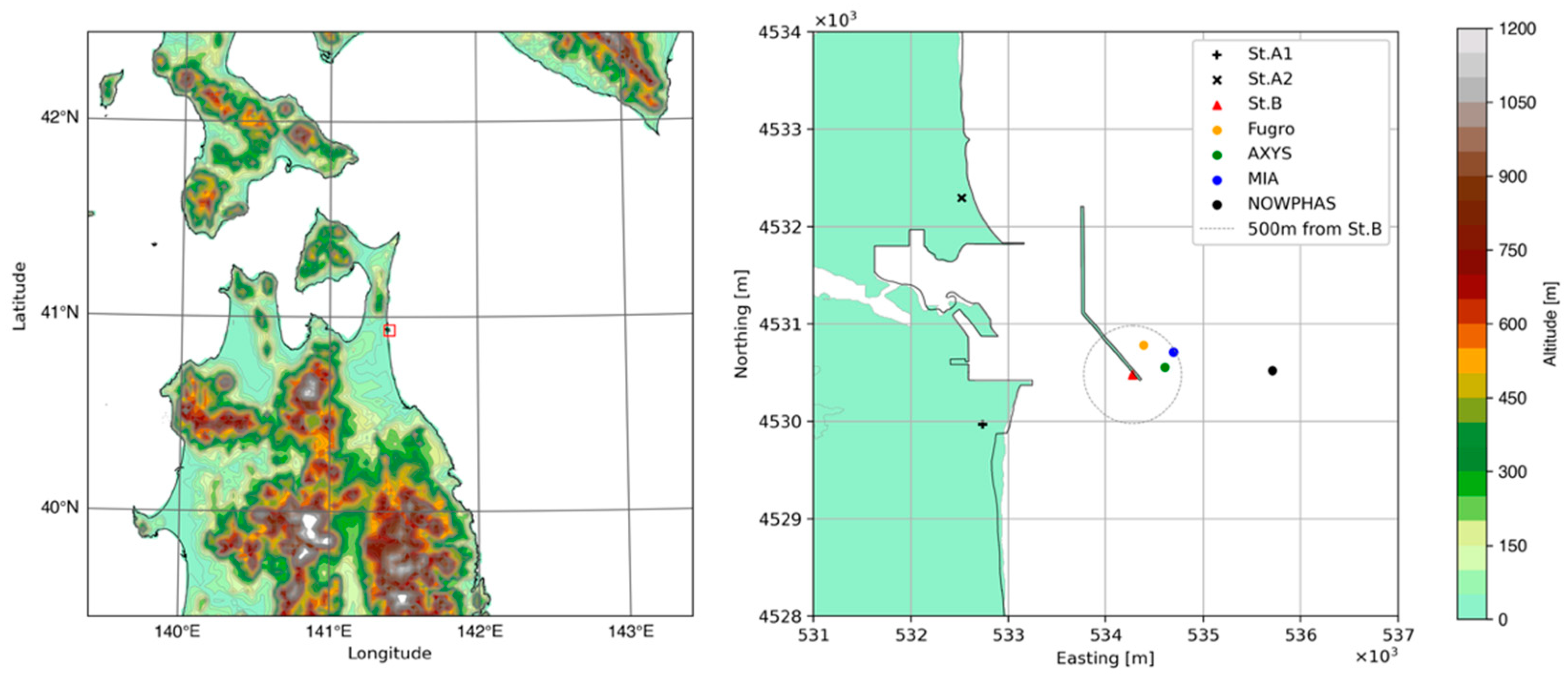
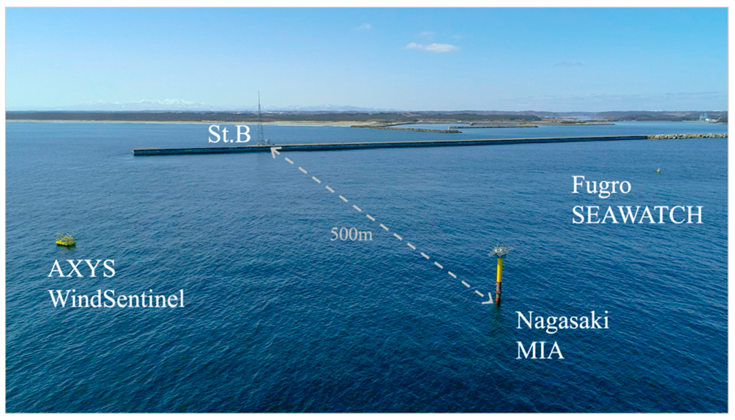
2.1. Mutsu-Ogawara Site
2.2. Reference Met Mast and VL on the Breakwater
2.3. Reference Wave Data
2.4. Floating LiDAR System Used for the Research
2.5. Key Performance Indicators and Other Evaluation Criteria
3. Results
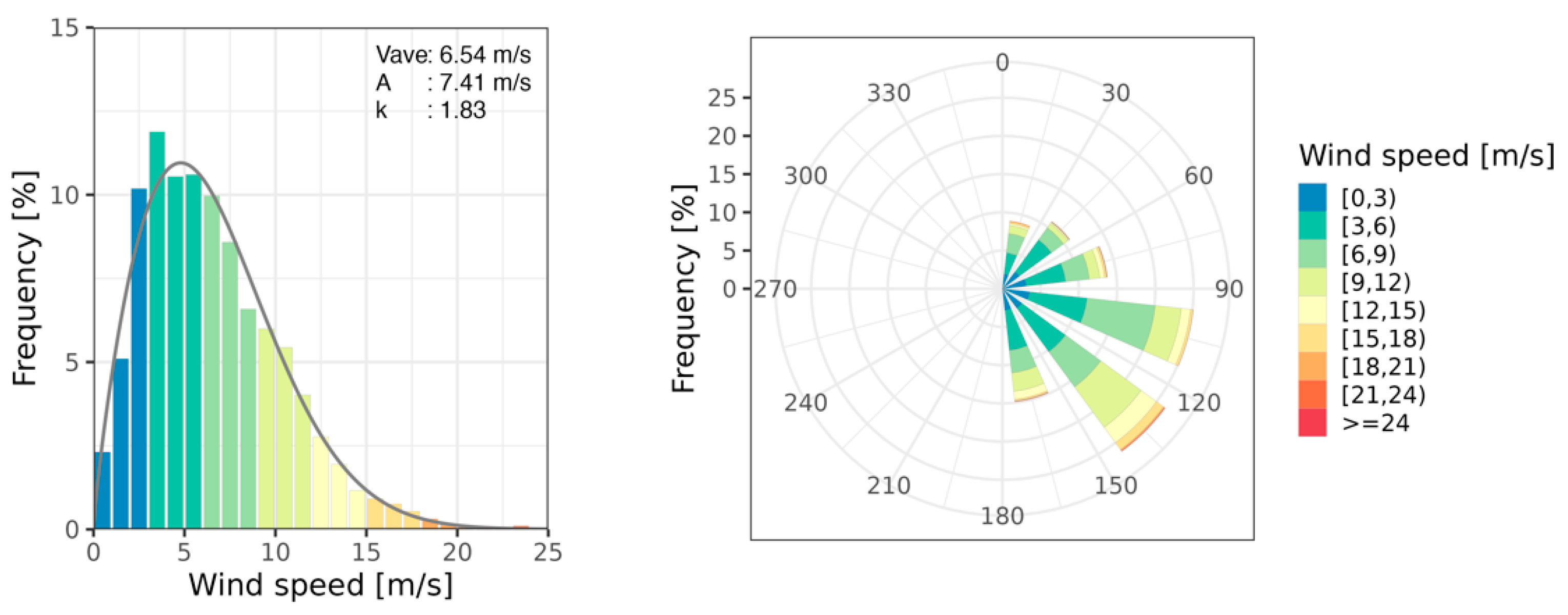
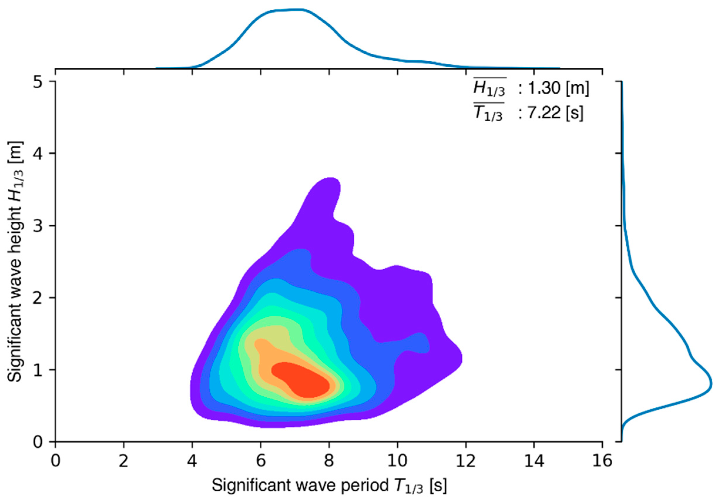
3.1. Metocean Conditions during the Verification
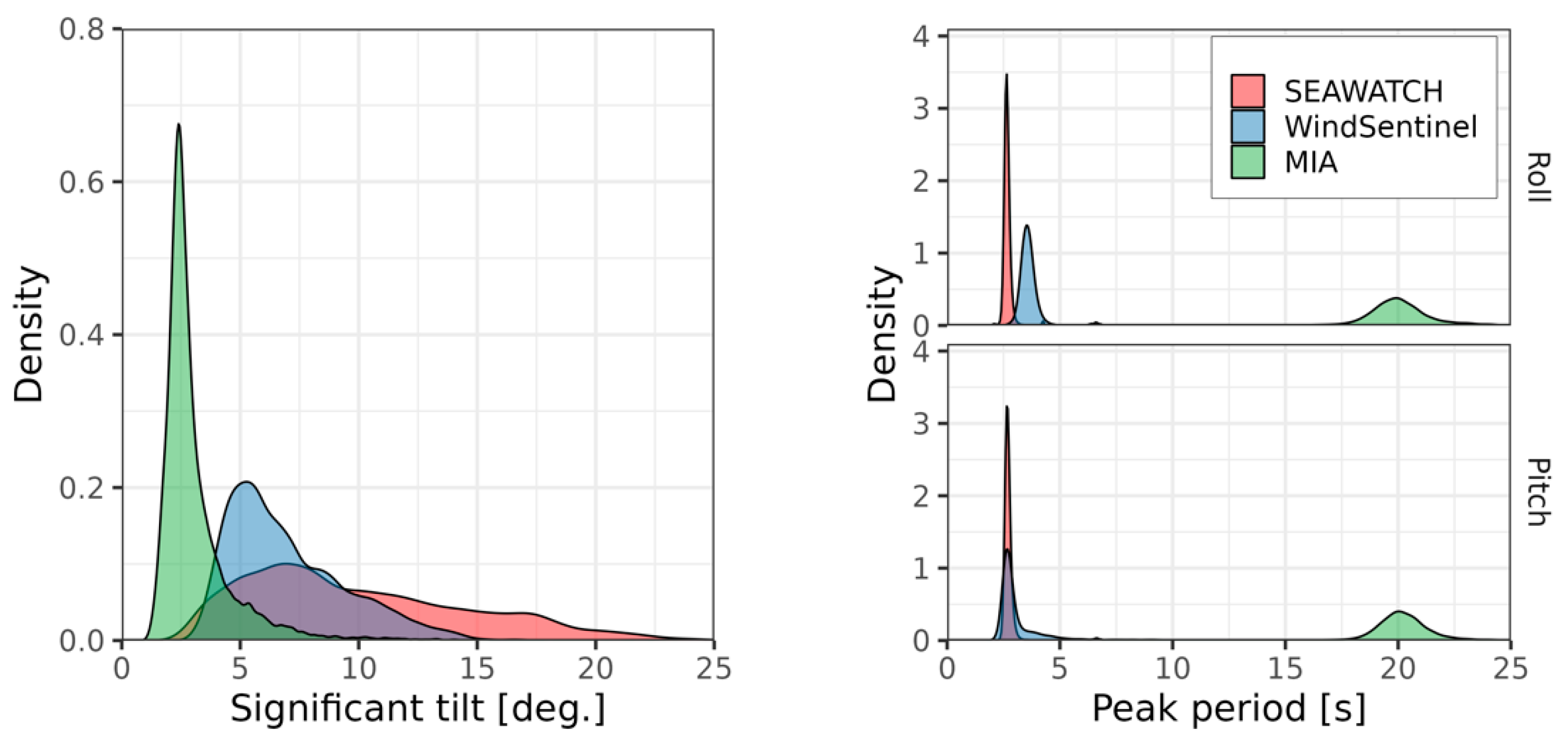
3.2. Analysis of the Buoy Motion
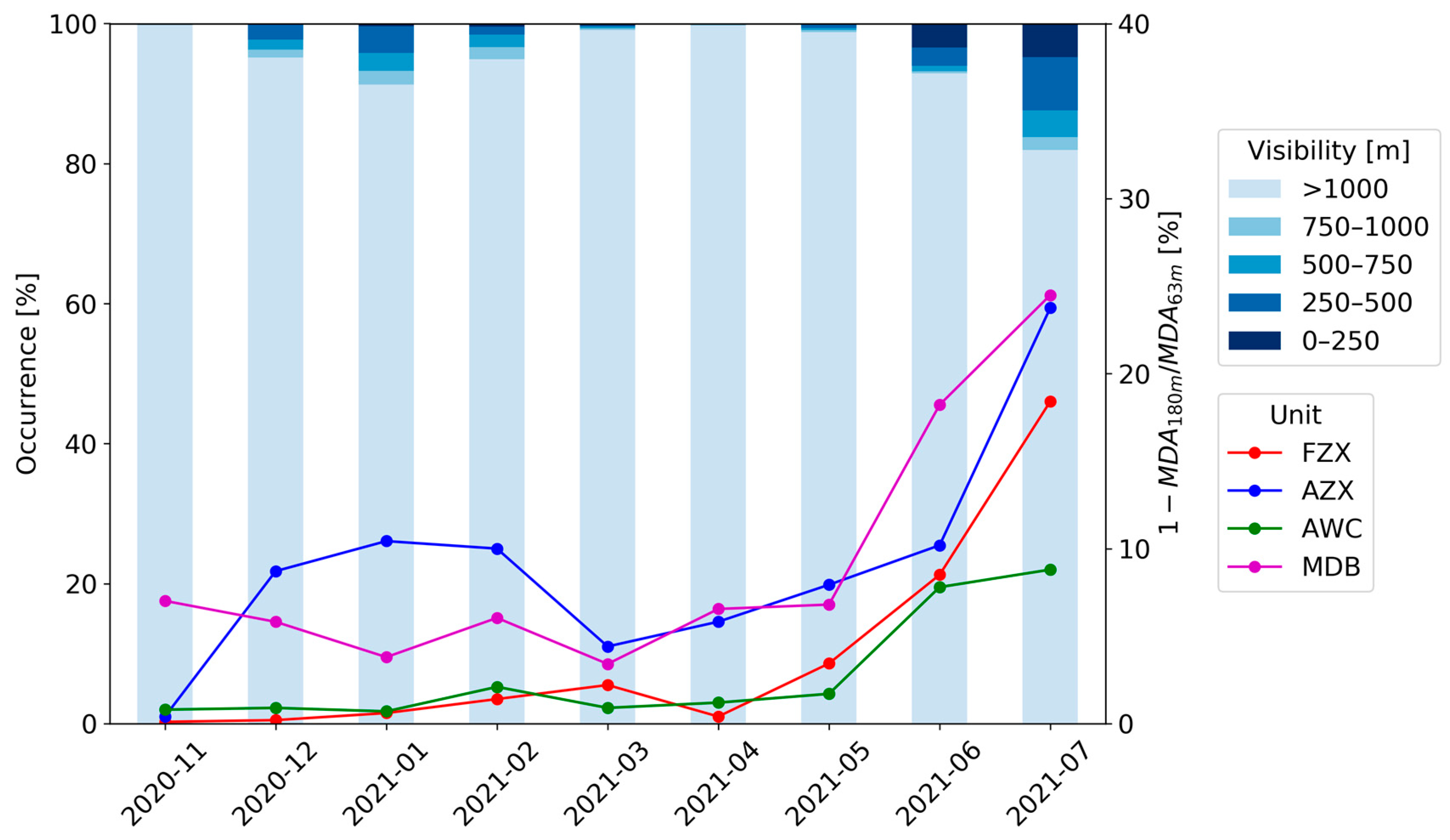
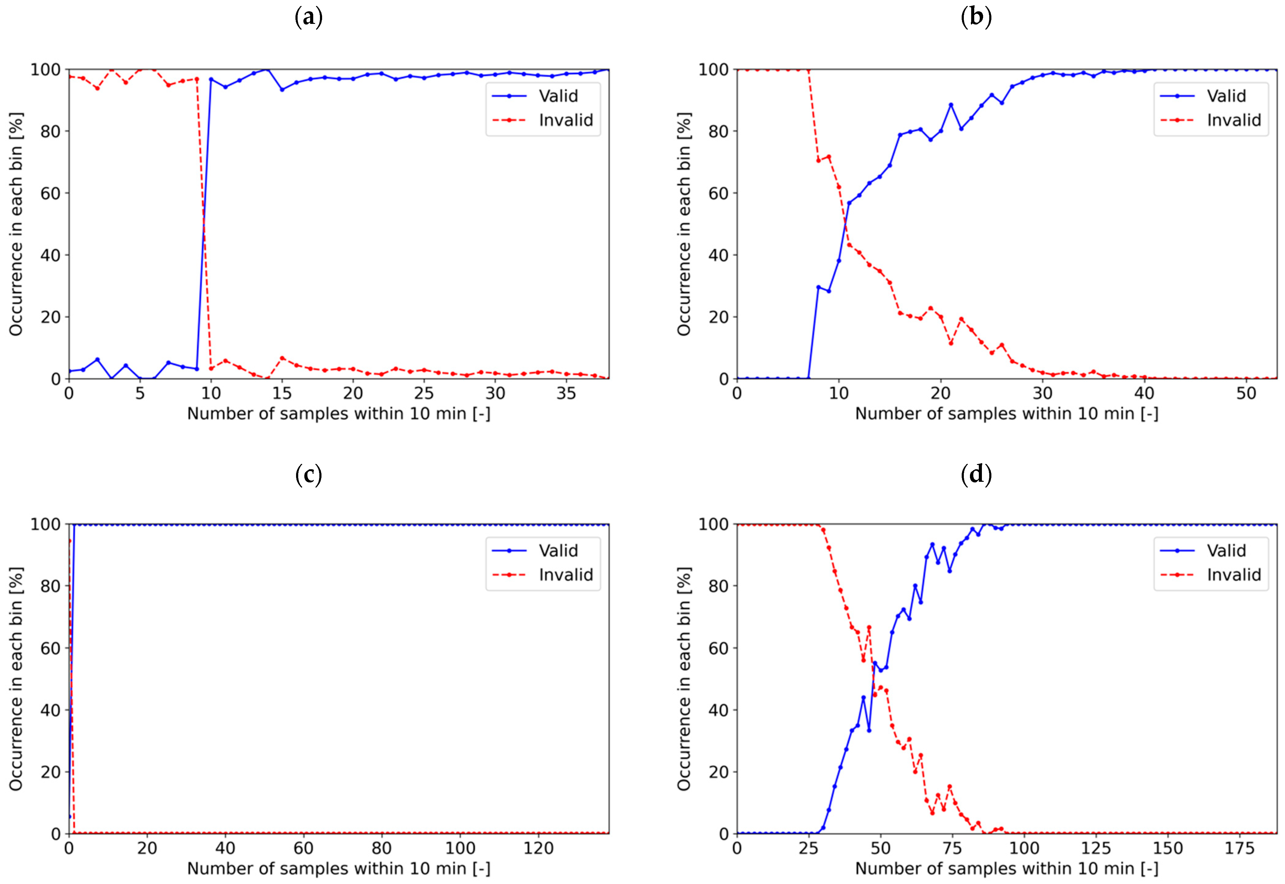
3.3. System and Data Availability
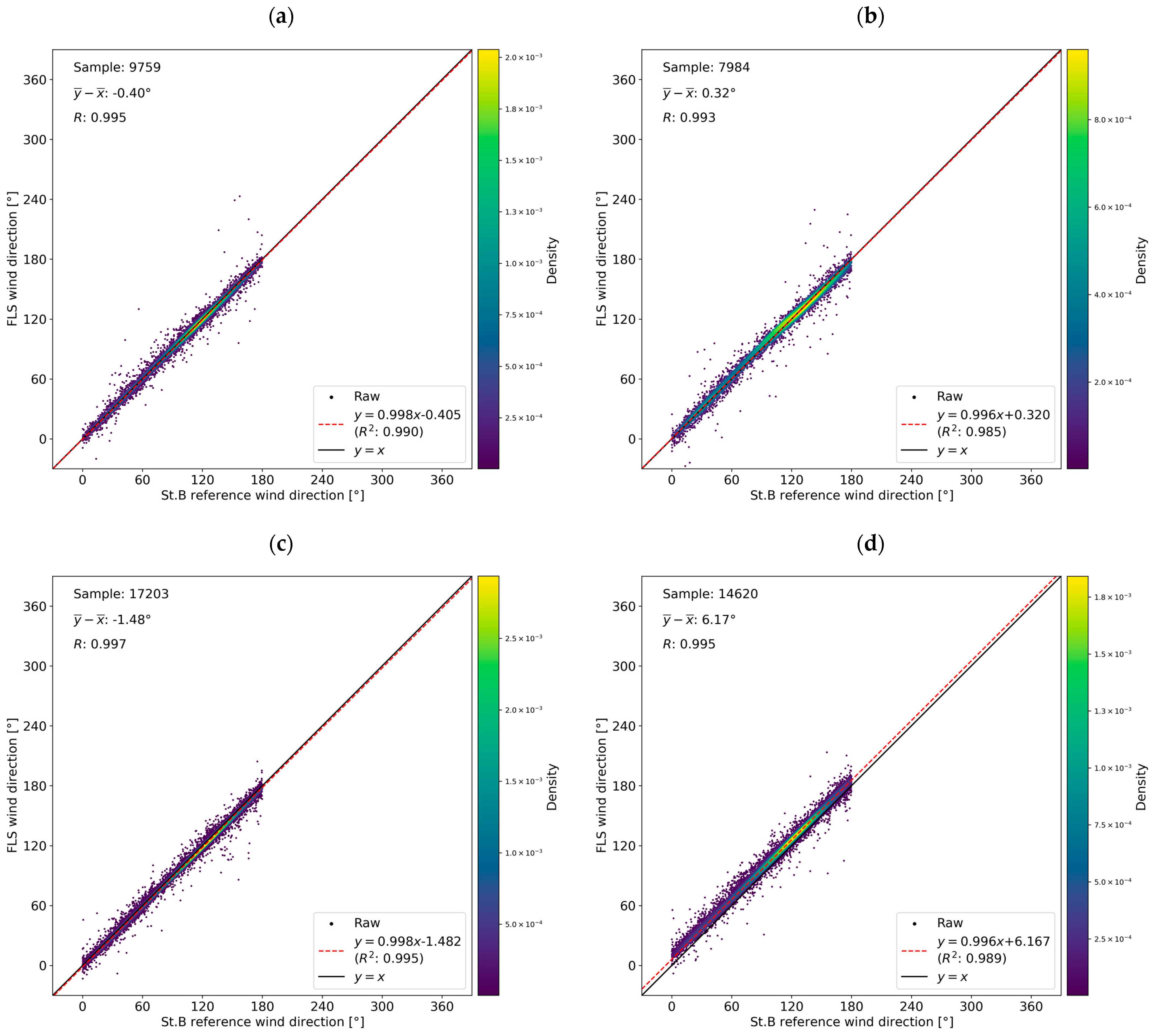
3.4. Ten-Minute Averaged Wind Speed and Direction
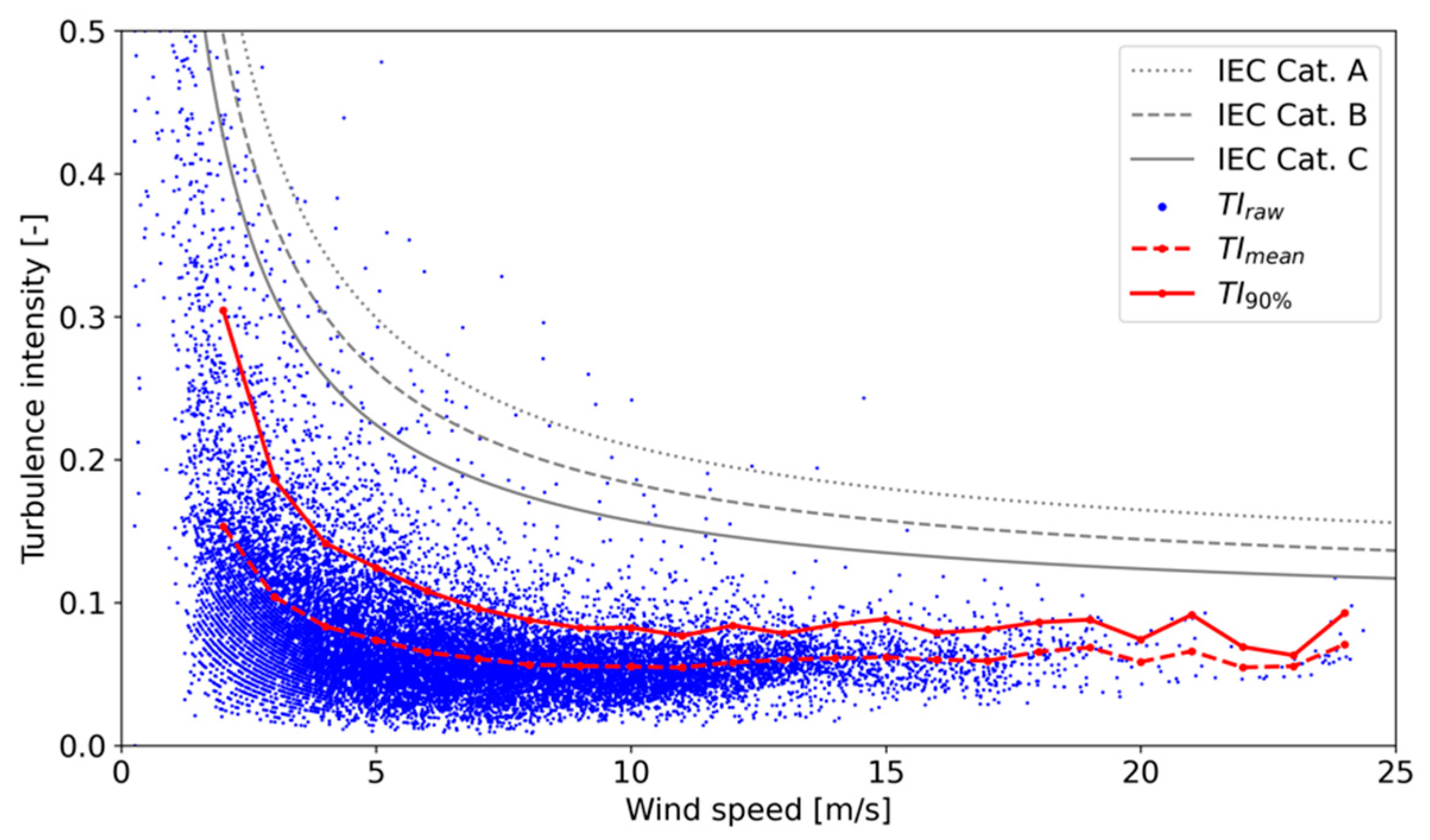
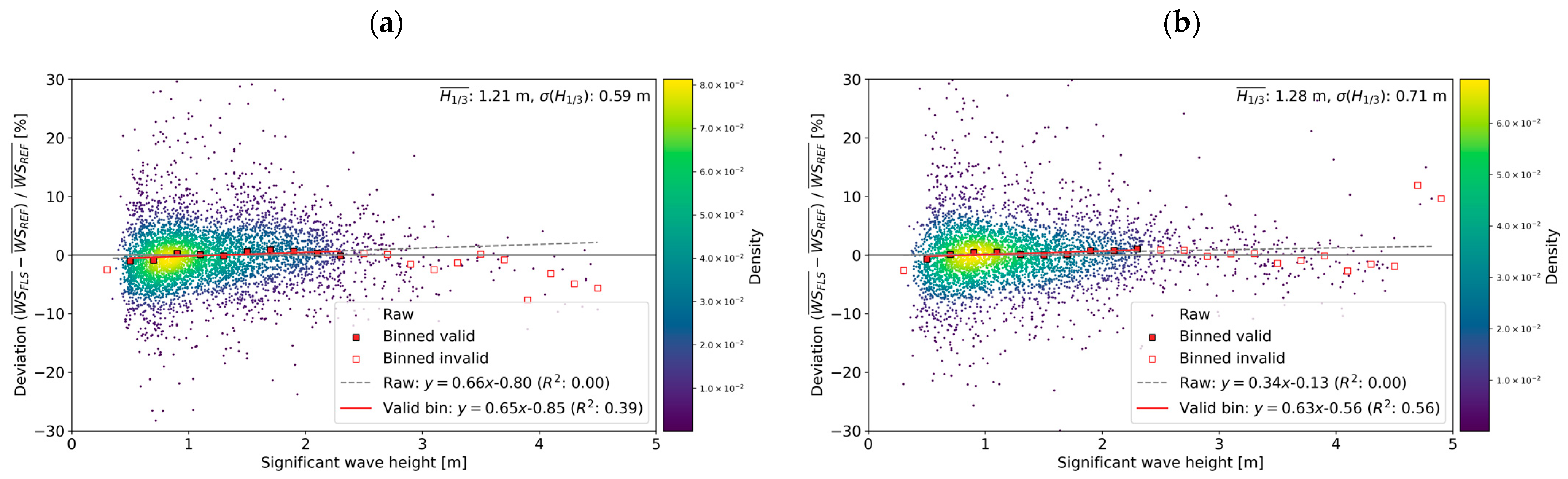
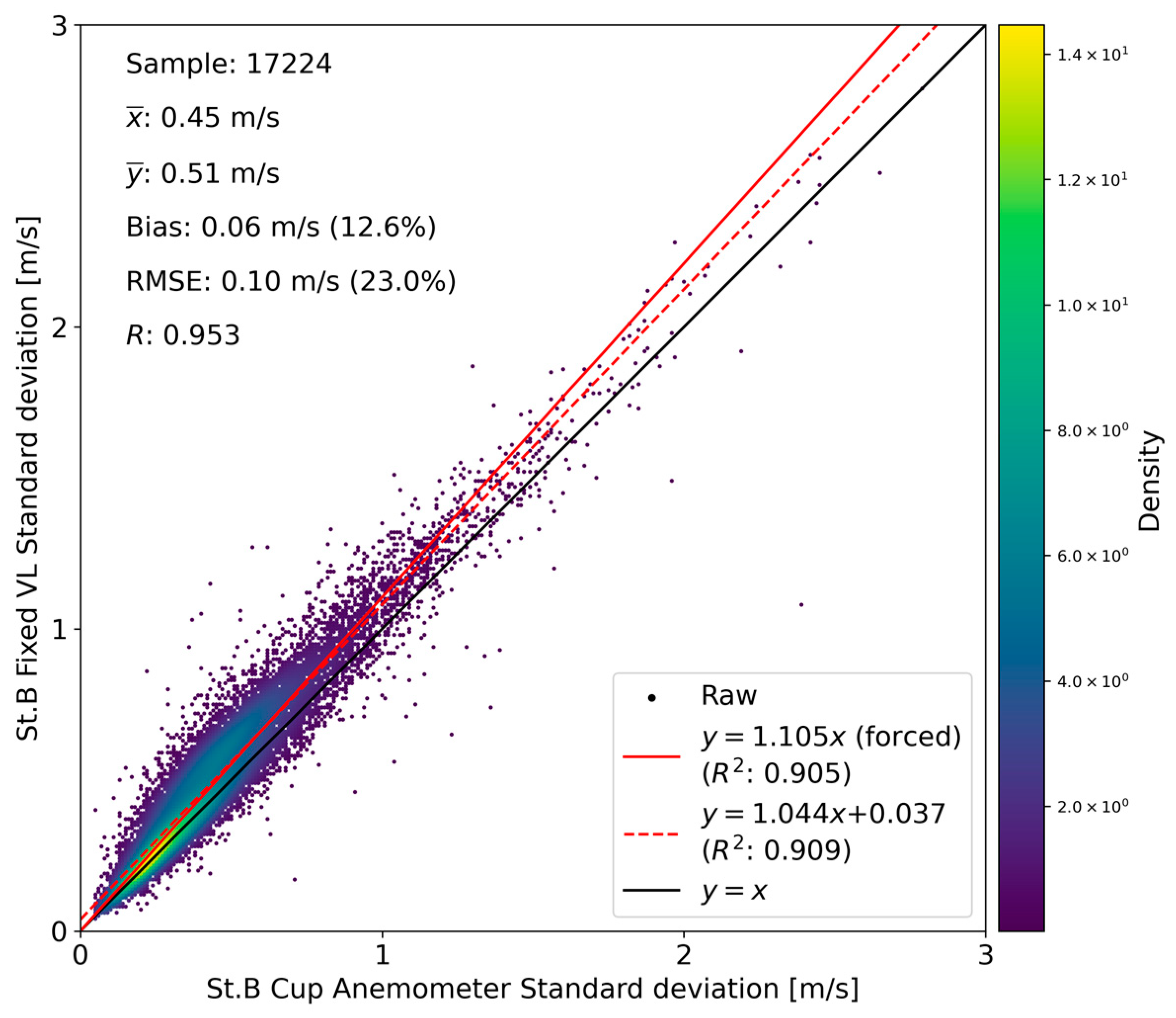
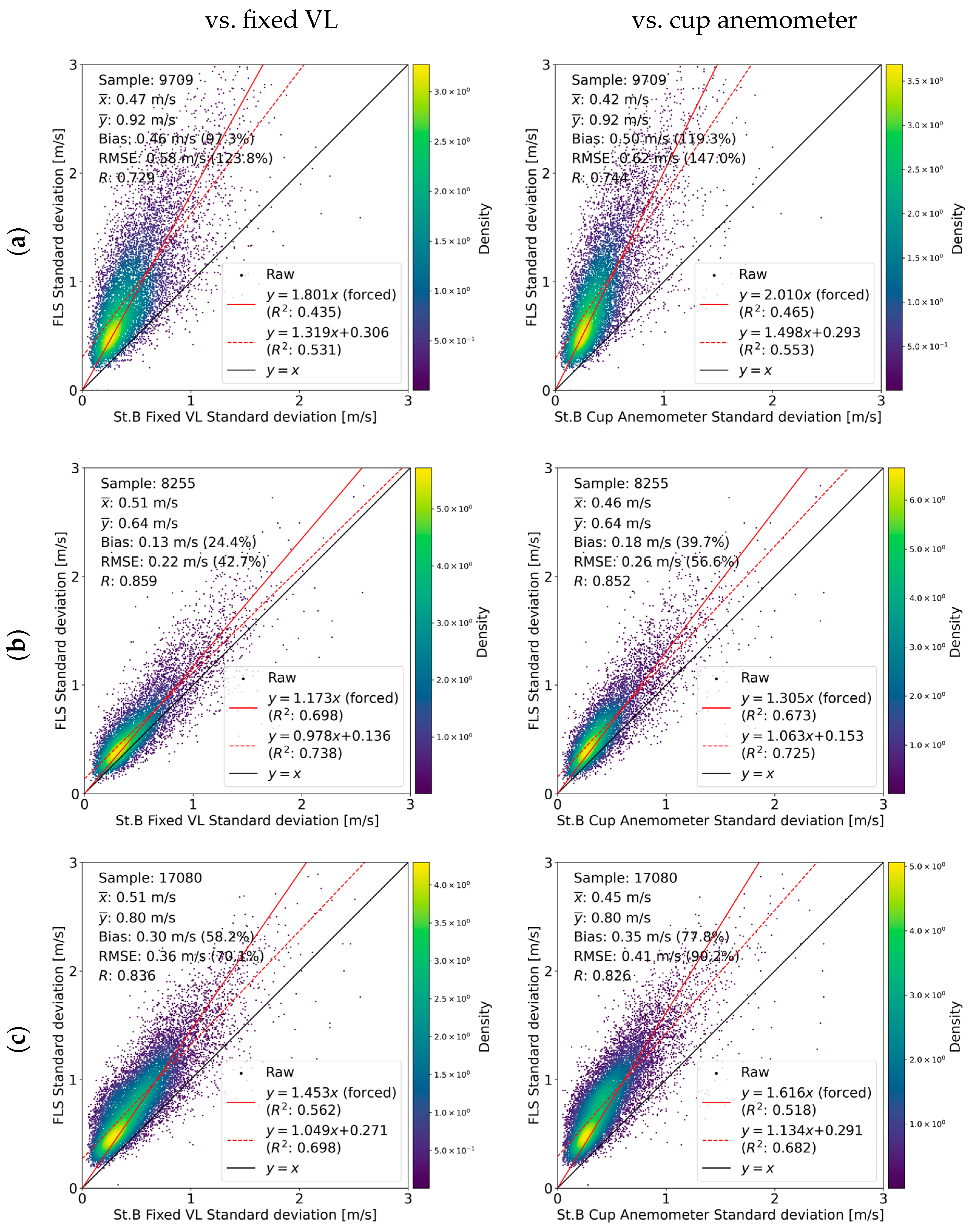
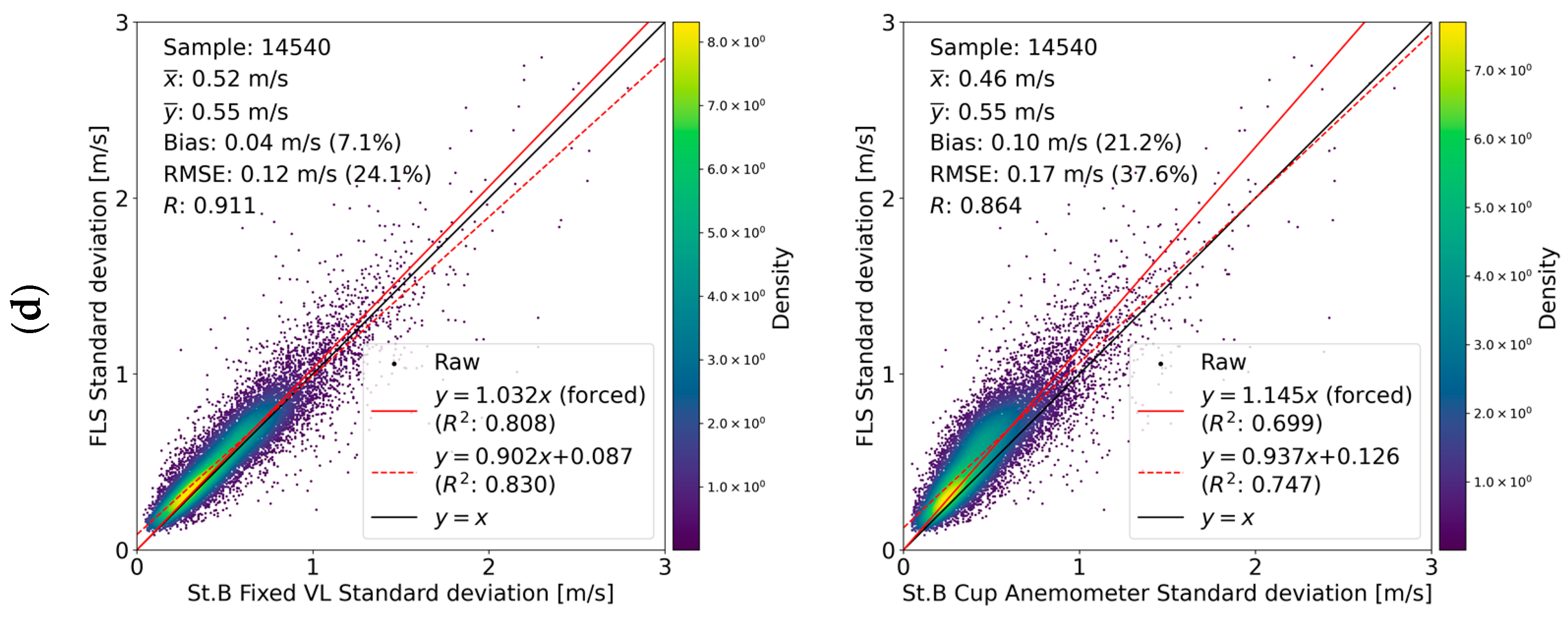
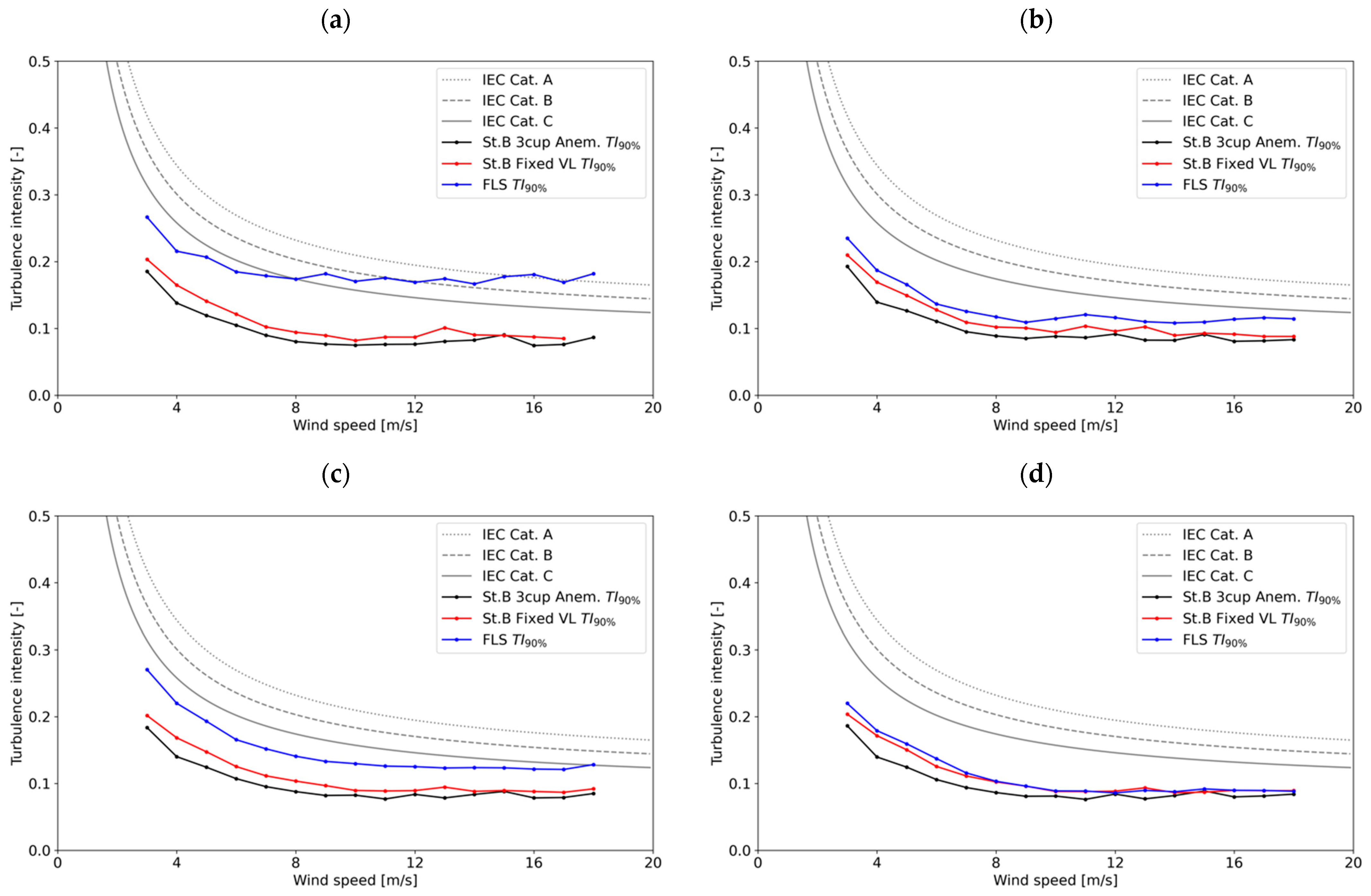
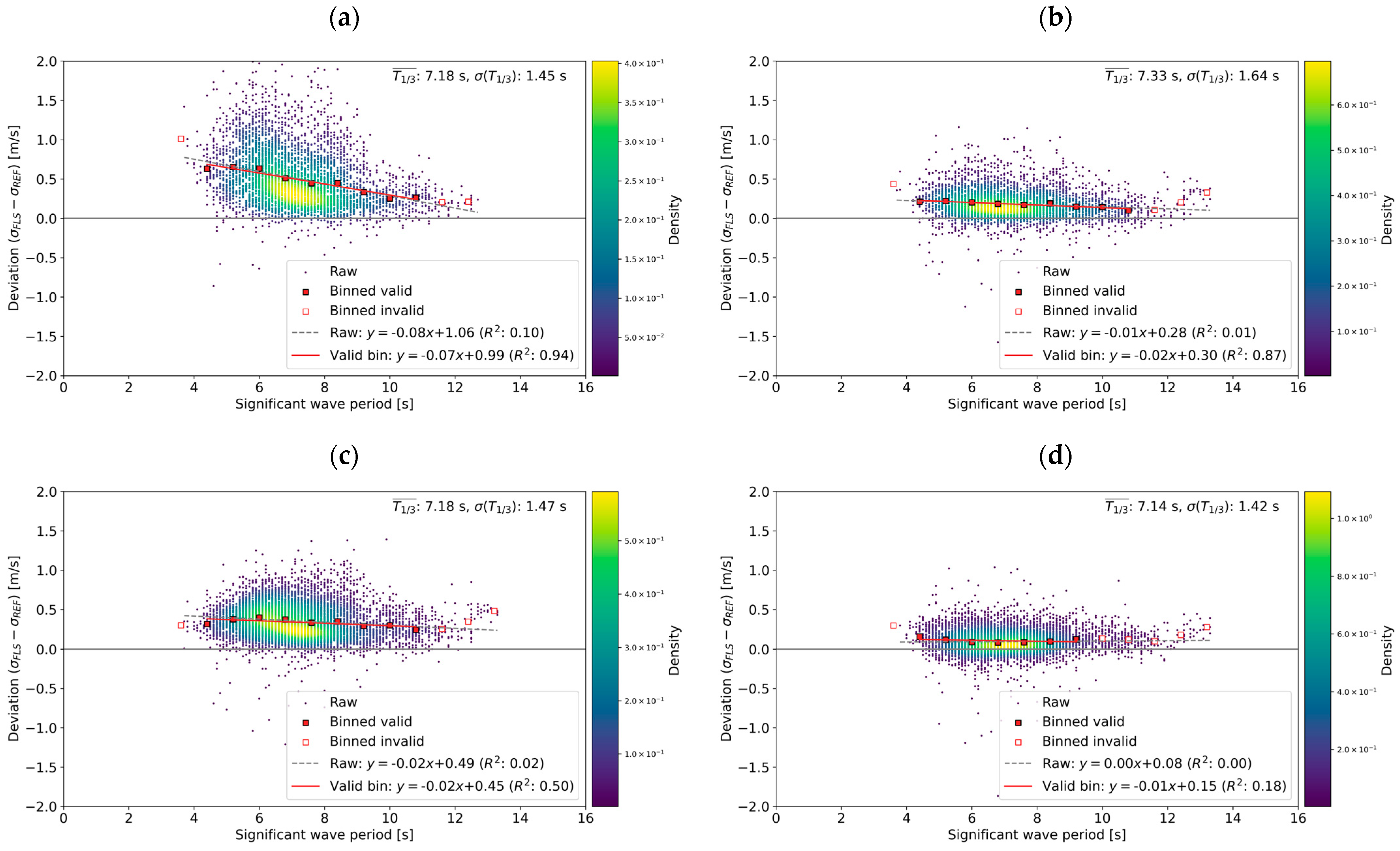
3.5. Ten-Minute Standard Deviation of Wind Speed and Turbulence Intensity
4. Discussion
5. Conclusions
Author Contributions
Funding
Data Availability Statement
Acknowledgments
Conflicts of Interest
References
- Gottschall, J.; Wolken-Möhlmann, G.; Viergutz, T.; Lange, B. Results and conclusions of a floating-lidar offshore test. Energy Procedia 2014, 53, 156–161. [Google Scholar] [CrossRef]
- Gottschall, J.; Gribben, B.; Stein, D.; Würth, I. Floating lidar as an advanced offshore wind speed measurement technique: Current technology status and gap analysis in regard to full maturity. Wiley Interdiscip. Rev. Energy Environ. 2017, 6, e250. [Google Scholar] [CrossRef]
- Vepa, K.S.; Duffey, T.; Paepegem, W.V. Gyroscope-based floating lidar design proposal for getting stable offshore wind velocity profiles. Sea Technol. 2016, 57, 41–43. [Google Scholar]
- Bischoff, O.; Würth, I.; Gottschall, J.; Gribben, B.; Hughes, J.; Stein, D.; Verhoef, H. IEA Wind, Expert Group Report on Recommended Practices, 18. Floating LiDAR Systems, 1st ed.; IEA Wind: Paris, France, 2017. [Google Scholar]
- Mathisen, J.-P. Measurement of Wind Profile with a Buoy Mounted Lidar. 2013, p. 19. Available online: https://www.sintef.no/globalassets/project/deepwind-2013/deepwind-presentations-2013/c2/mathisen-j.p_fugro-oceanor.pdf (accessed on 12 June 2024).
- Bischoff, O.; Würth, I.; Cheng, P.; Tiana-Alsina, J.; Gutiérrez, M. Motion effects on lidar wind measurement data of the EOLOS buoy. In Proceedings of the First International Conference on Renewable Energies Offshore, Lisbon, Portugal, 24–26 November 2014. [Google Scholar]
- Bischoff, O.; Yu, W.; Gottschall, J.; Cheng, P.W. Validating a simulation environment for floating lidar systems. J. Phys. Conf. Ser. 2018, 1037, 052036. [Google Scholar] [CrossRef]
- Bastigkeit, I.; Leimeister, M.; Watson, W.; Wolken-Möhlmann, G.; Gottschall, J. Enhanced design basis for offshore wind farm load calculations based on met-ocean data from a floating lidar system. J. Phys. Conf. Ser. 2021, 2018, 012008. [Google Scholar] [CrossRef]
- Carbon Trust Offshore Wind Accelerator (OWA). Roadmap for the Commercial Acceptance of Floating Lidar Technology. 2018. Available online: https://ctprodstorageaccountp.blob.core.windows.net/prod-drupal-files/documents/resource/public/Roadmap%20for%20Commercial%20Acceptance%20of%20Floating%20LiDAR%20REPORT.pdf (accessed on 12 June 2024).
- Viselli, A.; Filippelli, M.; Pettigrew, N.; Dagher, H.; Faessler, N. Validation of the first LiDAR wind resource assessment buoy system offshore the Northeast United States. Wind Energy 2019, 22, 1548–1562. [Google Scholar] [CrossRef]
- Gutiérrez-Antuñano, M.A.; Tiana-Alsina, J.; Rocadenbosch, F. Performance evaluation of a floating lidar buoy in nearshore conditions. Wind Energy 2017, 20, 1711–1726. [Google Scholar] [CrossRef]
- Gottschall, J.; Wolken-Möhlmann, G.; Lange, B. About offshore resource assessment with floating lidars with special respect to turbulence and extreme events. J. Phys. Conf. Ser. 2014, 555, 012043. [Google Scholar] [CrossRef]
- Gutiérrez-Antuñano, M.A.; Tiana-Alsina, J.; Salcedo, A.; Rocadenbosch, F. Estimation of the motion-induced-horizontal-wind-speed standard deviation in an offshore Doppler lidar. Remote Sens. 2018, 10, 2037. [Google Scholar] [CrossRef]
- Kelberlau, F.; Neshaug, V.; Lonseth, L.; Bracchi, T.; Mann, J. Taking the motion out of floating lidar: Turbulence intensity estimates with a continuous-wave wind lidar. Remote Sens. 2020, 12, 898. [Google Scholar] [CrossRef]
- Yamaguchi, A.; Ishihara, T. A new motion compensation algorithm of floating lidar system for the assessment of turbulence intensity. J. Phys. Conf. Ser. 2016, 753, 072034. [Google Scholar] [CrossRef]
- Ohsawa, T.; Shimada, S.; Kogaki, T.; Iwashita, T.; Konagaya, M.; Araki, R.; Imamura, H. Progress of NEDO project “Bottom fixed offshore wind farm development support project (Establishment of offshore wind resource assessment method)”. Proc. Jpn. Wind. Energy Symp. 2020, 42, 136–139. (In Japanese) [Google Scholar]
- The Nationwide Ocean Wave Information Network for Ports and HArbourS (NOWPHAS). Available online: https://www.mlit.go.jp/kowan/nowphas/index_eng.html (accessed on 29 March 2024).
- Konagaya, M.; Ohsawa, T.; Inoue, T.; Mito, T.; Kato, H.; Kawamoto, K. Land–Sea Contrast of Nearshore Wind Conditions: Case Study in Mutsu-Ogawara. SOLA 2021, 17, 234–238. [Google Scholar] [CrossRef]
- Türk, M.; Emeis, S. The dependence of offshore turbulence intensity on wind speed. J. Wind Eng. Ind. Aerodyn. 2010, 98, 466–471. [Google Scholar] [CrossRef]
- IEC 61400-12-1; Ed. 2.0 Wind Energy Generation Systems—Part 12-1: Power Performance Measurements of Electricity Producing Wind Turbines. International Electrotechnical Commission: Geneva, Switzerland, 2017.
- Wagner, R.; Mikkelsen, T.; Courtney, M. Investigation of Turbulence Measurements with a Continuous Wave, Conically Scanning LiDAR; Technical University of Denmark: Kongens Lyngby, Denmark, 2009; Technical Report Risø-R-1682(EN), Risø DTU. [Google Scholar]
- Sathe, A.; Mann, J. A review of turbulence measurements using ground-based wind lidars. Atmos. Meas. Tech. 2013, 6, 3147–3167. [Google Scholar] [CrossRef]
- Newman, J.F.; Clifton, A. An error reduction algorithm to improve lidar turbulence estimates for wind energy. Wind Energy Sci. 2017, 2, 77–95. [Google Scholar] [CrossRef]
- Kelberlau, F.; Mann, J. Better turbulence spectra from velocity–azimuth display scanning wind lidar. Atmos. Meas. Tech. 2019, 12, 1871–1888. [Google Scholar] [CrossRef]


| Period | From 24 November 2020 to 23 November 2021 |
| Location | On breakwater in Mutsu-Ogawara Port, Aomori Prefecture |
| Structure | Self-standing truss + tubular, up to 65 m in height |
| Main sensors | 63 m: three-cup anemometers (140° and 320° booms, NRG Systems Class 1) 61 m: Vane (50° boom, NRG Systems 200M) Sampling frequency: 1 Hz |
| Period | From 24 December 2020 to 23 November 2021 |
| Location | On the observation platform next to the St. B met mast |
| LiDAR type | Windcube V2.1 (Vaisala, formerly Leosphere) |
| Measurement heights | 50, 59, 63, 66, 80, 100, 120, 140, 160, 180, 200, and 250 m |
| Measurement parameters to be used | SD and TI at 63 m |
| Year | 2020 | 2021 | All | |||||||||||
|---|---|---|---|---|---|---|---|---|---|---|---|---|---|---|
| Month | Nov | Dec | Jan | Feb | Mar | Apr | May | Jun | Jul | Aug | Sep | Oct | Nov | |
| Met mast | 100.0 | 53.8 | 99.1 | 99.7 | 96.3 | 98.6 | 99.8 | 99.6 | 99.2 | 65.4 | 98.6 | 95.2 | 96.5 | 91.8 |
| Fixed VL | - | 66.2 | 99.8 | 99.9 | 99.9 | 99.9 | 96.7 | 100.0 | 99.8 | 69.7 | 99.5 | 99.9 | 94.3 | 91.9 |
| SEAWATCH | WindSentinel | MIA | |
|---|---|---|---|
| Image |  | 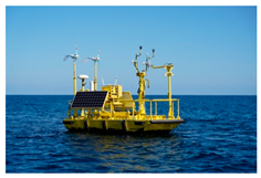 |  |
| Manufacturer | Fugro | AXYS Technologies | Nagasaki 5 companies |
| Shape | Round | Ship | Spar |
| Dimensions | Height: 7.2 m Diameter: ∅ 2.8 m | Height: 9 m Length: 6 m Width: 3.1 m | Height: 26 m Diameter: ∅ 1.0 m (above water level), ∅ 2.15 m (below water level) Maximum platform width: 5.5 m |
| Weight | Approximately 2.2 tons | Approximately 9 tons | Approximately 46 tons Platform: 2 tons Floater: 44 tons |
| Draft | Approximately 3 m | Approximately 2 m | Approximately 14.5 m |
| Material | Polyethylene, aluminum, and copper | Aluminum and copper | Copper and concrete |
| Mooring | Single-point catenary with a mid-float | Single point catenary | 3-point catenary |
| Drifting radius | Approximately 100 m | Approximately 120 m | Approximately 20 m |
| Mooring chain length | Approximately 85 m | Approximately 120 m | Approximately 320 m × 3 chains |
| LiDAR(s) | FZX: ZX300M (ZX Lidars) | AZX: ZX300M (ZX Lidars) AWC: Windcube (Vaisala) | MDB: DIABREZZA (Mitsubishi Electric) |
| Power | Fuel cell, photovoltaic (PV), and battery | Wind turbine, PV, battery, and diesel generator | Fuel cell, PV, and battery |
| Met. Parameters | Wind, temperature, and humidity | Wind, temperature, humidity, pressure, precipitation, and irradiance | Wind, temperature, humidity, and irradiance |
| Ocean parameters | Sea temperature, wave, and current | Sea temperature, wave, and current | Sea temperature |
| Height [m MSL] | Measurement | |||||
|---|---|---|---|---|---|---|
| St. B Met Mast | St. B VL | FZX | AZX | AWC | MDB | |
| 250 | ○ | ○ | Every 5 m up to 249 m | |||
| 220 | ○ | |||||
| 200 | ○ | ○ | ||||
| 180 | ○ | ○ | ○ | ○ | ○ (179 m) | |
| 160 | ○ | ○ | Every 5 m | |||
| 140 | ○ | ○ | ||||
| 120 | ○ | ○ | ○ | ○ | ○ (119 m) | |
| 100 or 102 | ○ (100 m) | ○ (100 m) | ○ (102 m) | ○ (100 m) | Every 5 m | |
| 80 | ○ | ○ | ||||
| 66 | ○ | |||||
| 61, 63 or 64 | Cup (63 m) Vane and sonic (61 m) | ○ (63 m) | ○ | ○ | ○ | ○ (64 m) |
| 59 | Cup/Propeller | ○ | Every 5 m from 54 m | |||
| 50 | Cup/Vane | ○ | ○ | |||
| 40 or 42 | ○ (40 m) | ○ (40 m) | ○ (42 m) | |||
| 25 | Cup | ○ | ○ | |||
| 12 | ○ | ○ | ||||
| Type | Description | Acceptance Criteria | |
|---|---|---|---|
| Stage 3 | Stage 2 | ||
| MSA1M | Monthly system availability | ≥90% | ≥85% |
| MPDA1M | Monthly post-processed data availability | ≥85% | ≥80% |
| Parameter | Condition | Type | Description | Acceptance Criteria | |
|---|---|---|---|---|---|
| Best Practice | Minimum | ||||
| Wind speed | ≥2 m/s and 4–16 m/s | Slope (Xmws) | Slope of single variant regression | 0.98–1.02 | 0.97–1.03 |
| R2 (R2mws) | Coefficient of determination from single variant regression | >0.98 | >0.97 | ||
| Bias (Bmws) | Relative mean error | Not defined | |||
| Wind direction | ≥2 m/s | Slope (Mmwd) | Slope of two-variant regression | 0.97–1.03 | 0.95–1.05 |
| Offset (OFFmwd) | Offset of two-variant regression | <5° | <10° | ||
| R2 (R2mwd) | Coefficient of determination from two-variant regression | >0.97 | >0.95 | ||
| Bin [m/s] | Range [m/s] | Samples [-] | ||||
|---|---|---|---|---|---|---|
| Start | End | FZX | AZX | AWC | MDB | |
| –2.0 | 0.0 | 2.0 | 727 | 673 | 1387 | 1003 |
| 2.5 | 2.0 | 3.0 | 1163 | 989 | 1906 | 1454 |
| 3.5 | 3.0 | 4.0 | 1324 | 1214 | 2219 | 1667 |
| 4.5 | 4.0 | 5.0 | 1152 | 1030 | 1960 | 1588 |
| 5.5 | 5.0 | 6.0 | 1244 | 1034 | 1946 | 1644 |
| 6.5 | 6.0 | 7.0 | 1199 | 968 | 1820 | 1613 |
| 7.5 | 7.0 | 8.0 | 929 | 681 | 1582 | 1485 |
| 8.5 | 8.0 | 9.0 | 699 | 489 | 1230 | 1104 |
| 9.5 | 9.0 | 10.0 | 576 | 399 | 1121 | 1006 |
| 10.5 | 10.0 | 11.0 | 409 | 316 | 1019 | 957 |
| 11.5 | 11.0 | 12.0 | 308 | 286 | 753 | 690 |
| 13.0 | 12.0 | 14.0 | 365 | 425 | 883 | 789 |
| 15.0 | 14.0 | 16.0 | 167 | 257 | 389 | 337 |
| 16.0– | 16.0 | - | 224 | 258 | 375 | 286 |
| Total | - | - | 10,486 | 9019 | 18,590 | 15,623 |
| 2020–2021 | System Availability [%] | Data Availability (Relative to System Availability) [%] | ||
|---|---|---|---|---|
| 63 m | 120 m | 180 m | ||
| November | 100.0 | 99.0 (99.0) | 98.9 (98.9) | 98.9 (98.9) |
| December | 100.0 | 99.3 (99.3) | 99.2 (99.2) | 99.0 (99.1) |
| January | 100.0 | 99.3 (99.3) | 99.1 (99.1) | 98.7 (98.7) |
| February | 100.0 | 99.7 (99.7) | 98.9 (98.9) | 98.3 (98.3) |
| March | 100.0 | 99.7 (99.7) | 98.9 (98.9) | 97.5 (97.5) |
| April | 43.6 | 43.1 (98.8) | 43.2 (98.9) | 42.9 (98.4) |
| May | 100.0 | 98.9 (98.9) | 97.1 (97.1) | 95.5 (95.5) |
| June | 100.0 | 96.4 (96.4) | 91.0 (91.0) | 88.2 (88.2) |
| July | 78.9 | 71.6 (90.7) | 61.6 (78.1) | 58.4 (74.0) |
| August | 0.0 | 0.0 (-) | 0.0 (-) | 0.0 (-) |
| September | No measurement | |||
| October | ||||
| November | ||||
| Overall | 80.6 | 79.0 (98.0) | 76.9 (95.4) | 75.8 (94.0) |
| 2020–2021 | System Availability [%] | Data Availability (Relative to System Availability) [%] | ||
|---|---|---|---|---|
| 63 m | 120 m | 180 m | ||
| November | 99.8 | 98.0 (98.2) | 97.7 (97.9) | 97.6 (97.8) |
| December | 99.8 | 98.5 (98.7) | 93.4 (93.6) | 89.9 (90.1) |
| January | 99.9 | 97.7 (97.8) | 92.1 (92.2) | 87.5 (87.6) |
| February | 99.8 | 92.8 (93.0) | 87.7 (87.9) | 83.6 (83.7) |
| March | 77.3 | 77.2 (99.8) | 75.2 (97.3) | 73.8 (95.4) |
| April | 96.2 | 95.8 (99.6) | 93.2 (96.9) | 90.2 (93.8) |
| May | 97.9 | 96.3 (98.3) | 91.9 (93.8) | 88.7 (90.5) |
| June | 74.4 | 70.1 (94.2) | 65.6 (88.1) | 62.9 (84.6) |
| July | 28.5 | 27.0 (94.7) | 22.2 (77.9) | 20.6 (72.2) |
| August | 0.0 | 0.0 (-) | 0.0 (-) | 0.0 (-) |
| September | 0.0 | 0.0 (-) | 0.0 (-) | 0.0 (-) |
| October | 16.7 | 16.4 (98.1) | 14.8 (88.7) | 14.1 (84.5) |
| November | 82.2 | 78.8 (95.8) | 77.5 (94.2) | 75.8 (92.1) |
| Overall | 64.5 | 62.7 (97.2) | 59.6 (92.5) | 57.5 (89.1) |
| 2020–2021 | System Availability [%] | Data Availability (Relative to System Availability) [%] | ||
|---|---|---|---|---|
| 63 m | 120 m | 180 m | ||
| November | 100.0 | 100.0 (100.0) | 100.0 (100.0) | 99.2 (99.2) |
| December | 99.9 | 99.9 (100.0) | 99.9 (100.0) | 99.1 (99.1) |
| January | 99.9 | 99.9 (100.0) | 99.8 (100.0) | 99.1 (99.3) |
| February | 74.4 | 74.4 (100.0) | 74.4 (100.0) | 72.9 (97.9) |
| March | 100.0 | 100.0 (100.0) | 100.0 (100.0) | 99.1 (99.1) |
| April | 100.0 | 99.9 (99.9) | 99.9 (99.9) | 98.7 (98.7) |
| May | 100.0 | 99.8 (99.8) | 99.7 (99.8) | 98.1 (98.1) |
| June | 100.0 | 100.0 (100.0) | 98.4 (98.4) | 92.2 (92.2) |
| July | 99.9 | 99.9 (100.0) | 99.6 (99.7) | 91.1 (91.2) |
| August | 100.0 | 100.0 (100.0) | 99.5 (99.5) | 94.5 (94.5) |
| September | 100.0 | 100.0 (100.0) | 100.0 (100.0) | 99.7 (99.8) |
| October | 99.8 | 99.8 (100.0) | 99.8 (100.0) | 99.4 (99.6) |
| November | 99.9 | 99.9 (100.0) | 99.8 (99.9) | 98.6 (98.7) |
| Overall | 98.0 | 98.0 (100.0) | 97.7 (99.8) | 95.4 (97.3) |
| 2020–2021 | System Availability [%] | Data Availability (Relative to System Availability) [%] | ||
|---|---|---|---|---|
| 64 m | 119 m | 179 m | ||
| November | 100.0 | 99.8 (99.8) | 98.4 (98.4) | 92.8 (92.8) |
| December | 96.5 | 96.2 (99.7) | 95.6 (99.0) | 90.6 (93.9) |
| January | 35.1 | 35.1 (100.0) | 34.7 (98.8) | 33.8 (96.2) |
| February | 83.5 | 82.9 (99.3) | 81.7 (97.9) | 77.9 (93.3) |
| March | 69.9 | 69.7 (99.7) | 69.4 (99.2) | 67.4 (96.3) |
| April | 86.9 | 86.2 (99.2) | 85.4 (98.2) | 80.5 (92.7) |
| May | 29.4 | 28.9 (98.5) | 28.6 (97.4) | 27.0 (91.8) |
| June | 68.3 | 68.3 (99.9) | 64.7 (94.6) | 55.8 (81.7) |
| July | 99.9 | 97.5 (97.6) | 92.5 (92.7) | 73.6 (73.7) |
| August | 99.9 | 99.4 (99.5) | 95.9 (96.0) | 85.6 (85.7) |
| September | 99.9 | 99.5 (99.6) | 98.3 (98.4) | 94.7 (94.8) |
| October | 100.0 | 99.2 (99.3) | 97.2 (97.2) | 90.5 (90.5) |
| November | 95.7 | 95.5 (99.8) | 92.7 (96.8) | 84.6 (88.4) |
| Overall | 80.4 | 79.8 (99.3) | 78.0 (97.1) | 71.9 (89.4) |
| Type | Condition | FZX | AZX | AWC | MDB | Acceptance Criteria |
|---|---|---|---|---|---|---|
| Slope (Xmws) | ≥2 m/s | 0.999 | 1.001 | 1.017 | 1.023 | Best Practice: 0.98–1.02 Minimum: 0.97–1.03 |
| 4–16 m/s | 1.001 | 1.004 | 1.020 | 1.024 | ||
| R2 (R2mws) | ≥2 m/s | 0.991 | 0.992 | 0.993 | 0.990 | Best Practice: >0.98 Minimum: >0.97 |
| 4–16 m/s | 0.985 | 0.987 | 0.989 | 0.985 | ||
| Bias (Bmws) [%] | ≥2 m/s | 0.0 | 0.3 | 1.7 | 2.3 | Not defined |
| 4–16 m/s | 0.1 | 0.4 | 2.0 | 2.4 |
| Type | Condition | FZX | AZX | AWC | MDB | Acceptance Criteria |
|---|---|---|---|---|---|---|
| Slope (Mmwd) | ≥2 m/s | 0.998 | 0.996 | 0.998 | 0.996 | Best Practice: 0.97–1.03 Minimum: 0.95–1.05 |
| Offset (OFFmwd) | −0.405 | 0.320 | −1.482 | 6.167 | Best Practice: <5° Minimum: <10° | |
| R2 (R2mwd) | 0.990 | 0.985 | 0.995 | 0.989 | Best Practice: >0.97 Minimum: >0.95 |
Disclaimer/Publisher’s Note: The statements, opinions and data contained in all publications are solely those of the individual author(s) and contributor(s) and not of MDPI and/or the editor(s). MDPI and/or the editor(s) disclaim responsibility for any injury to people or property resulting from any ideas, methods, instructions or products referred to in the content. |
© 2024 by the authors. Licensee MDPI, Basel, Switzerland. This article is an open access article distributed under the terms and conditions of the Creative Commons Attribution (CC BY) license (https://creativecommons.org/licenses/by/4.0/).
Share and Cite
Uchiyama, S.; Ohsawa, T.; Asou, H.; Konagaya, M.; Misaki, T.; Araki, R.; Hamada, K. Accuracy Verification of Multiple Floating LiDARs at the Mutsu-Ogawara Site. Energies 2024, 17, 3164. https://doi.org/10.3390/en17133164
Uchiyama S, Ohsawa T, Asou H, Konagaya M, Misaki T, Araki R, Hamada K. Accuracy Verification of Multiple Floating LiDARs at the Mutsu-Ogawara Site. Energies. 2024; 17(13):3164. https://doi.org/10.3390/en17133164
Chicago/Turabian StyleUchiyama, Shogo, Teruo Ohsawa, Hiroshi Asou, Mizuki Konagaya, Takeshi Misaki, Ryuzo Araki, and Kohei Hamada. 2024. "Accuracy Verification of Multiple Floating LiDARs at the Mutsu-Ogawara Site" Energies 17, no. 13: 3164. https://doi.org/10.3390/en17133164