Article

Localization of Partial Discharges in Hydrogenerators by Ozone Emission

by
Victor Dmitriev
1,
Rodrigo M. S. de Oliveira
1,*,
Licinius D. S. de Alcantara
2 and
Gustavo G. Girotto
1
1
Instituto de Tecnologia (ITEC), Federal University of Pará (UFPA), Rua Augusto Correa n° 01, Belem 66075-110, Brazil
2
Instituto Ciberespacial (ICIBE), Federal Rural University of Amazon (UFRA), Avenida Presidente Tancredo Neves, n∘ 2501, Belem 66077-830, Brazil
*
Author to whom correspondence should be addressed.
Energies 2024, 17(13), 3173; https://doi.org/10.3390/en17133173
Submission received: 20 May 2024 / Revised: 12 June 2024 / Accepted: 17 June 2024 / Published: 27 June 2024

Abstract

:
We suggest a new method of localization of partial discharges in high-power electrical systems. Ozone in a hydrogenerator is produced by chemical reactions induced by partial discharges in the stator region. The transport of ozone in an operating hydrogenerator is analyzed using a computational fluid dynamics model. The main aim of this work is to evaluate the ozone distribution in the generator radiators. Ozone sources are introduced into the stator model in different positions to analyze their effect on the measured values at the sensing points of radiators. Our results demonstrate a possibility of localization of partial discharges in hydrogenerator stator bars by ozone emission.

1. Introduction

Power outages caused by hydrogenerator failures are costly and disruptive. Predictive maintenance based on online partial discharge (PD) testing has emerged as a powerful tool to avoid failures. Researchers focused on PD levels as an indicator of insulation weakness in hydrogenerators. PDs occur when high voltage stresses create tiny sparks within the insulation, indicating potential problems. PDs are provoked by various issues: poor impregnation, faulty coatings, inadequate coil spacing, loose windings, overheating, contamination, and even foreign objects like screws [1].
Monitoring PDs has become a common method for assessing generator health. When assessing insulation conditions in the equipment, like stator windings, technical staff often use offline PD measurements during testing [2]. The International Electrotechnical Commission (IEC) recommends using low frequencies (below 3 MHz) for the electrical tests due to the electrical properties of the windings, since they act like capacitors and inductors [3]. However, high-frequency components of the PD signal can weaken depending on where the sensor is placed relative to the PD source. This means that using a wider range of frequencies for detection leads to a more accurate identification of PD activity, as confirmed by several studies [4,5].
Online PD testing offers several advantages since real-time data can be acquired continuously during normal operation [6]. It allows analysis and diagnostics during operation to identify issues early and plan corrective actions to minimize downtime [7]. Proactive maintenance also prevents unexpected failures, reducing the risk of unscheduled outages.
However, it is important to mention that PD tests are not immune to errors and imprecision. Their primary role is to alert operators about potential problems, identify the cause, and isolate the issue [8].
Partial discharges within hydrogenerators manifest through various phenomena, including electromagnetic (EM) and acoustic emissions, along with chemical reactions like ozone formation. However, for practical measurement, electrical methods dominate the field. In the most common and straightforward approach, capacitive couplers [9] are used, but alternative solutions are directional couplers [10,11,12] and antennas [13].
Accurately pinpointing the location of PDs within a hydrogenerator from their electromagnetic emissions presents a significant challenge. This difficulty exists in an individual bar and aggravates in groups of bars. The complexity stems from the excitation of high-frequency EM waves by PD events, which propagate within the bar’s insulation and diffract in conductive parts and bar ends. Furthermore, EM waves radiate from the bar into the surrounding air and reflect from neighboring structures, creating numerous electromagnetic couplings [13]. As a consequence, sensors register intricate transient electromagnetic signals (voltages and currents) that necessitate sophisticated analysis for PD localization.
The presence of ozone within air-cooled generators and motors serves as a strong indicator of partial discharge activity [14]. Studies suggest that deterioration of semiconductive coatings is the primary culprit for ozone generation. However, the rate of ozone formation is influenced by numerous variables and may not always offer a reliable assessment of the state’s health. While the direct correlation with total PDs might not exist, ozone concentrations can provide valuable insights into specific types of surface PDs, including slot discharges, corona at coating junctions, and PDs between coils or connections. Therefore, monitoring ozone becomes a valuable tool for predictive maintenance.
A significant challenge in using ozone for PD localization lies in ventilation. Airflow significantly impacts concentrations, as demonstrated by a laboratory experiment where ozone levels dropped dramatically with increased airflow [15]. This imposes some limitations on the absolute ozone level measurements.
Air velocity, temperature, and voltage are all likely to play a role, with the specific impact depending on the specific operating conditions of the hydrogenerator. In [16], a developed ozone prediction model based on the mechanism of ozone generation in a corona discharge region shows that ozone concentration decays as the air velocity increases. This occurs because the gas velocity becomes the main factor in governing the ozone transport characteristics. At even higher air velocities, the gas with diluted ozone will experience increased turbulence. This turbulence can enhance the mixing of the ozone with the surrounding air, leading to faster diffusion and a wider distribution of the ozone. For example, large-scale climate patterns like El Niño Southern Oscillation (ENSO) can significantly impact the ozone in the atmosphere. El Niño events are linked to a decrease in ozone concentration specifically within the lower-middle stratosphere [17].
Higher temperatures generally increase the kinetic energy of gas molecules, including ozone. This increased energy leads to more frequent collisions between molecules, promoting faster diffusion [18,19]. An hydrogenerator operating at a higher voltage may lead to the production of more partial discharges and ozone molecules. However, the impact on diffusion is less straightforward. The increased energy imparted to the gas and the local increase of temperature [20] during the discharge process could promote diffusion.
Combining ozone data with PD levels, machine load, voltage, and temperature leads to a more comprehensive diagnostic panorama. For instance, rising PD levels with stable ozone concentrations could suggest internal insulation PD. Furthermore, ozone measurements can complement traditional PD tests, particularly in high humidity conditions where surface PDs through capacitive couplers become less detectable [21].
Typical ozone concentrations in generators range from dozens to hundreds of ppb (parts per billion). Therefore, initial measurements should utilize equipment with high precision in this range. The measurement range of various ozone sensors using different techniques for measurement was reported in [22]. Portable devices often rely on optical sensors with wide dynamic ranges. However, if electrochemical sensors are chosen, establishing a baseline measurement beforehand is crucial to selecting the sensor with the most appropriate range.
While the importance of ozone monitoring in hydrogenerators for detecting partial discharges is well-established, the definition of the sensor positions remains open. This lack of guidance poses challenges for accurate and reliable diagnostics, potentially hindering effective maintenance and insulation condition assessment. Therefore, investigation of the influence of the sensor position on ozone concentration measurements and PD detection accuracy is a relevant subject of scientific research. Using computational fluid dynamic (CFD) modeling of a hydrogenerator in operation, this work aims to analyze the influence of the positions of the internal sources of ozone produced by PDs on the detection of ozone concentrations at the radiator outlets. This allows one to associate distinct insulation defects in the generator with ozone concentration measurements.

2. Materials and Methods

Figure 1a is a photo of a typical hydrogenerator. Our structure model for the following analysis is presented in Figure 1b. The structure was created by the COMSOL Multiphysics 5.5 software using as a base a generating unit from the Brazilian Campos Novos hydroelectric plant.
The hydrogenerator stator winding is made up of 378 coil-type bars with an interior made of copper and an external surface with a semiconductor coating layer. The bars have dimensions of 672.7 mm × 3.961 m, and their details are shown in Figure 2. The material of the floor and walls of the generator were modeled using concrete. The floor has an octagonal shape with edges measuring 5.385 m, and the walls are 4.20 m high. The radiators have dimensions of 1.72 m × 4.20 m. They are made of copper, and their grid structure was approximated by a surface as defined in [24].
The air directors guide the air flow from the rotor to the radiators. These elements are made of stainless steel and have a wedge-like shape with side dimensions of 1.615 m, an external side at a radius of 5.468 m, and a height of 4.20 m. The stator core is made up of 47.2 mm thick sections of stainless steel sheets with a spacing between the sections for ventilation of 15 mm. Its total height is 2.658 m, and it has an external radius of 4.180 m and an internal radius of 3.820 m. To accommodate the stator bars, the structure has grooves measuring 128 mm × 33.3 mm and teeth measuring 128 mm × 30.2 mm. Finally, the rotor was modeled by a cylinder with a radius of 3.8075 m, a height of 3.3418 m, and an external surface with epoxy resin coating.

3. Fluid Dynamics Theory

3.1. Basic Equations and Boundary Conditions

Viscous incompressible fluids flow as described in the steady-state Navier-Stokes equations [25] of conservation of momentum given by
( u m · ) u m = 1 ρ 0 p + ν 2 u m + a ,
· u m = 0 ,
where ∇ is the vetorial operator = def ( / x , / y , / z ) , u m = ( u , v , w ) is the flow speed in m/s, and u , v , and w are the components of the velocity vector; p is the scalar pressure field in Pa, ρ 0 is the fluid density in kg/m3, ν is the kinematic viscosity of the fluid in m2/s, and a is the gravitational acceleration in m/s2.
On rigid surfaces, walls are considered impermeable and non-slippery. Therefore, the following boundary conditions can be used:
u n = 0 ,
and
u t = 0 ,
where the subscripts n and t indicate, respectively, the components of u m normal and tangential to a considered solid surface. Equation (3) guarantees impermeability, and (4) ensures that the obstacle is not slippery.
The mass conservation law [25] for a chemical species i in the steady state is given by
· J i + u m · c i = R i ,
and
J i = D i c i ,
where c i is the species concentration given in mol/m2, J i is the diffusion flux vector given in mol/(m2s), u m is the average mass velocity given in m/s, R i is the reaction rate for the species given in mol/(m3s), and D i is the diffusion coefficient given in m2/s.
Equations (1), (2), (5) and (6) are solved numerically by COMSOL Multiphysics software version 5.5 using the finite element method.

3.2. Fluid Dynamics Applied to Ozone

The parameter R i associated with ozone generation in (5) can be calculated by [26]
R i = η · P m · V O 3 ,
where η is the ozone generation efficiency, P is the power of the partial discharges, m is the molar mass of ozone, whose value is 47.998 g/mol [27], and V O 3 is the volume of the region where ozone is generated.
The distribution of ozone in an environment can be calculated with (5); however, part of this ozone ends up being eliminated due to reactions with molecules of the environment and reactions with the surfaces. The flux of ozone deposition on surfaces can be calculated by [28]
J s = γ < v B > 4 C | y = 2 3 l ,
where J s is the net flux of species to the surface calculated at a small reference distance y from the reaction surface, as established in [28]. γ is the mass accommodation coefficient between ozone and the deposition surface and is defined as the fraction of all ozone molecules colliding with the surface that undergo deposition. C is the ozone concentration, l is the mean molecular free path with a value of 6.5 × 10⁻⁸ m at 293 K and 1 atm, and < v B > is the Boltzmann velocity for ozone, given by
< v B > = 8 k T π m ,
where k is the Boltzmann constant equals to 1.38 × 10⁻²³ JK−1 and T is the ambient temperature in K. Considering T = 293 K, the Boltzmann velocity for ozone has the value of 3.6 × 10² m/s.
According to [18,28,29], the diffusion coefficient D i for ozone in (6) is 1.82 × 10⁻⁵ m2/s in the air under atmospheric conditions at sea level and a temperature around 298 K. The parameter γ in (8) depends on the surface material; see Table 1.

4. Numerical Model

4.1. A General Description

The effect of the rotor rotation in the model is described through the air velocity boundary condition. The two velocity components were defined: the first one is the angular velocity of 87.344 m/s, which corresponds to the velocity on the rotor surface for rotation of 200 RPM (revolutions per minute), and the radius of the rotor equals to 3.8075 m.
The second velocity is the radial one. In order to define this velocity on the rotor surface, we have measured the radial velocity at the outlet of a radiator in the working generator unit. It has the value of 3 m/s. However, the air guides confine the flow path, enhancing the velocity. Therefore, the radial velocity at the rotor surface is lower than at the radiator exit, so it was evaluated as 2.2 m/s. For each radiator and its circular section in the hydrogenerator, a specific label from R 1 to R 8 was assigned, as illustrated in Figure 3.
In order to demonstrate the suggested method of PD localization in the stator winding, ten ozone sources corresponding to PD locations were defined (see Figure 4 and Table 2). The exact geometry and positioning of one of the ozone sources are shown in Figure 5. To represent the ozone sources, square cuboids measuring 20.2 × 20.2 × 15 mm were placed and activated individually in each simulation.
Each ozone source has a fixed value of ozone reaction rate, which represents a steady-state regime value. Square sources are used to represent averaged emissions instead of using irregularly shaped sources. By averaging the emission rate over the area of the square source, the model can capture the overall impact of the source without requiring a detailed representation of its geometry. Square sources are relatively straightforward to implement in a CFD model compared to more complex shapes. This kind of approximation can be beneficial when working with structures with complex geometries.

4.2. Numerical Mesh

A finite element mesh for the simulations was generated using a pre-defined calibration method for fluid dynamics models in COMSOL Multiphysics. In this way, the mesh was built with 6,116,483 tetrahedral elements, of which 2,025,344 were triangles, 698,438 edge elements, and 152,484 vertex elements. To refine the mesh in the critical ozone source region, a maximum edge length of 7.5 mm was used. The computational mesh is shown in Figure 6.
The simulations were carried out using two workstations working in parallel, each equipped with an AMD Ryzen 9 5950X 16-Core processor and 128 GB of RAM. The execution time of each simulation varied between 12 and 14 h, and they required approximately 124 GB of RAM.

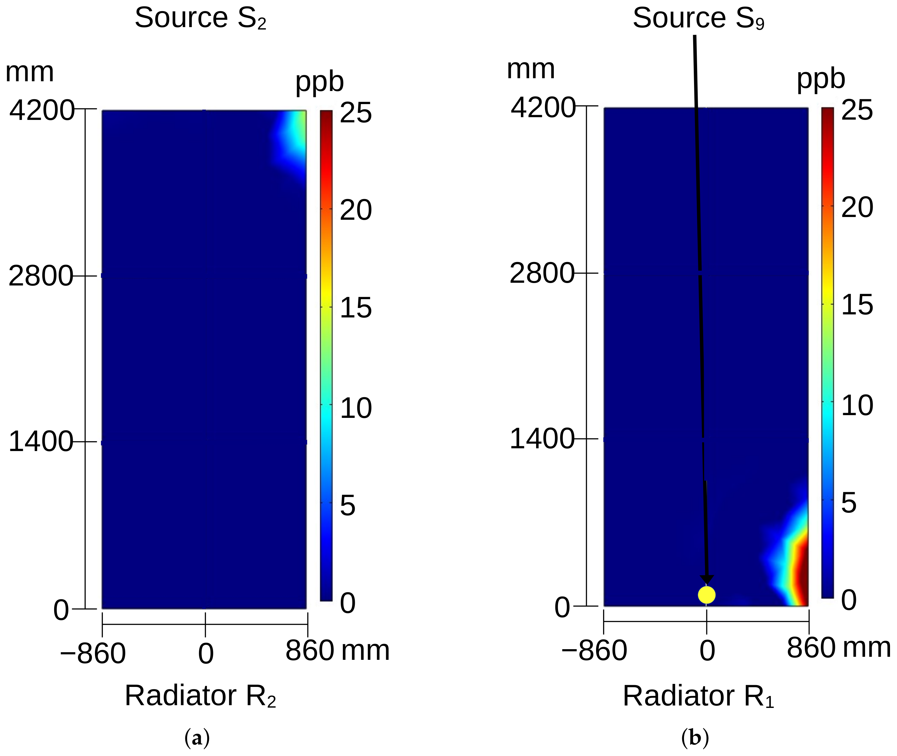
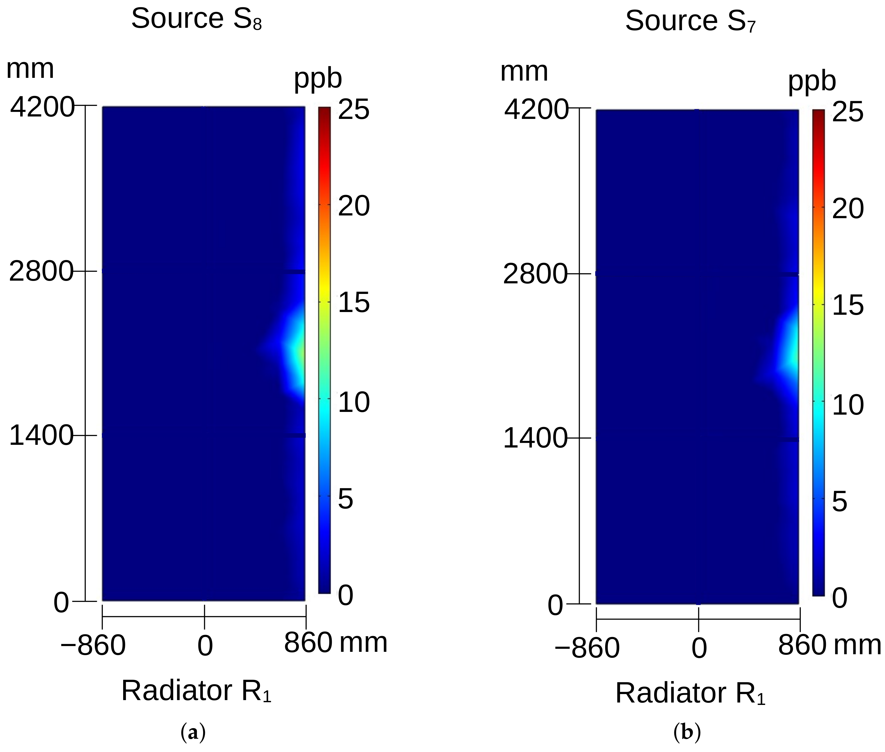
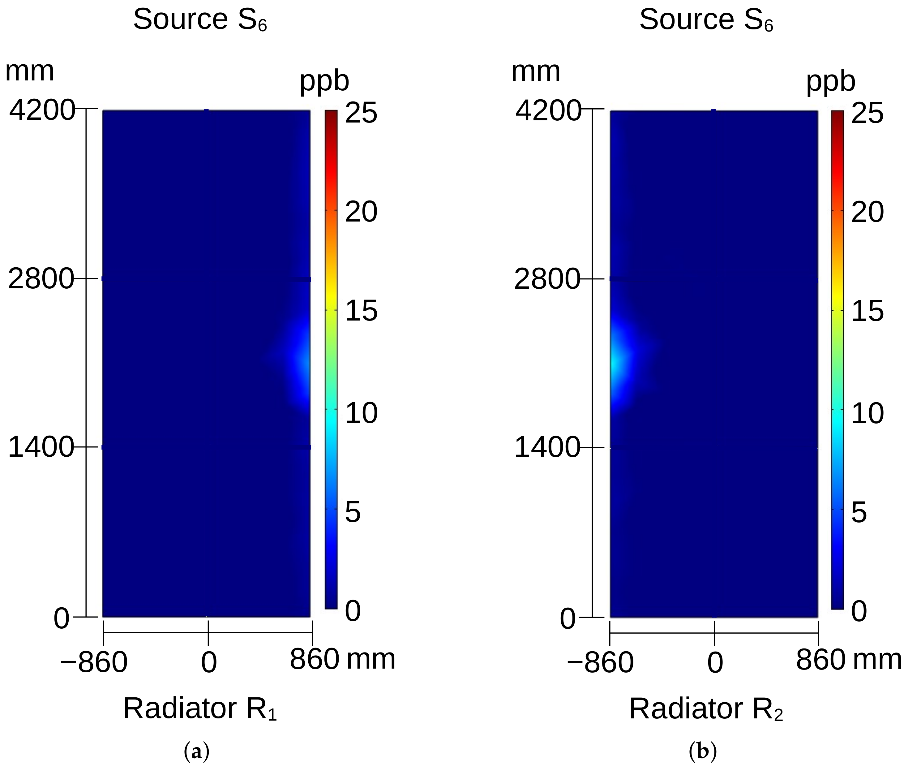
5. Results and Discussion

In order to validate the numerical results that will be presented below, experiments were carried out to verify the accuracy of the developed CFD model. With the impossibility of carrying out such experiments in a real hydrogenerator, simpler laboratory tests were conducted using a stator bar in an acrylic chamber. The results demonstrating a good accordance of the calculated and measured data are presented in Appendix A.
Calculation of the airflow is important for understanding how ozone is transported from PD sources to the radiator outlets. Figure 7 shows the air velocity field in the horizontal plane z = 2100 mm, in the proximity of radiator R 1 . The air flow, which is more intense near the rotor, is affected by the stator bars and the air directors.
Figure 8, Figure 9, Figure 10, Figure 11, Figure 12 and Figure 13 show the distribution of ozone concentration on the radiators’ output planes measured in ppb (part per billion) when a specific ozone source is activated. When source S 1 is activated, the generated ozone is transported and divided between radiators R 1 and R 2 . This occurs due to the high angular component of the velocity in the upper and also in the lower regions of the generator. Therefore, even if the source S 1 is located in the central angular region of the radiator R 1 , the velocity angular component is strong enough to capture and divide ozone between two radiators (Figure 8a,b). When source S 2 is activated, the corresponding output ozone distribution is observed mostly in the upper right part of radiator R 2 ; see Figure 9a. In this case, ozone is not present in radiator R 1 .
When source S 3 or S 4 or S 5 is activated, ozone appears at the center of radiator R 1 (see Figure 10b and Figure 11a,b), but this source remains undetectable at radiator R 2 . In these cases, the ρ coordinate of the sources only impacts the intensity of detected ozone. However, the intensity is also influenced by the power of partial discharges occurring in the source, which is determined by the severity of the insulation problem.
Sources S 6 , S 7 , or S 8 are located close to the air director nozzle. Figure 13 shows ozone distributions on radiator R 1 when sources S 7 and S 8 are activated. In the case of a DP source with a smaller ρ coordinate (source S 6 ), ozone can be detected on the right edge of radiator R 1 as well as on the left edge of radiator R 2 ; see Figure 13a,b. Due to proximity of the source to the rotor, where the air speed is greater, ozone is carried to the neighboring radiator, where it can be detected.
As already mentioned, in the top and bottom regions of the hydrogenerator there are the ends of the ferromagnetic core and the stator bars, so that in these regions the air flow is freer from obstacles, and thus the air velocity vectors have more intense azimuthal and vertical components in the vicinity of radiators. This can also be noted when the sources S 9 and S 10 are activated, as shown in Figure 9a,b. In the case of source S 10 , its effect is perceived mostly on the lower right part of the radiator R 2 , showing that the azimuthal component of air velocity had a stronger effect transporting ozone also to the radiator of the adjacent sector (Figure 10a).

6. Conclusions

The study utilizes a CFD model to simulate airflow and the ozone distribution in the radiators of high-power hydrogenerators. Validation of the model by laboratory experiments confirms its effectiveness. The location of an ozone source within the hydrogenerator directly affects the distribution of ozone in the radiator. By activating different sources, we observed ozone concentration in distinct areas of the radiator. In some cases, ozone appears in two adjacent radiators simultaneously.
The configuration of stator bars, air directors, and rotation of the rotor have influence on the air velocity, especially near the radiators. A more unobstructed airflow path near the top and bottom of the hydrogenerator leads to stronger azimuthal and vertical air velocity components. This results in an indirect trajectory of ozone transport that can lead to maximum ozone concentration in the radiator of the adjacent sector. Thus, maps of correspondence between positions of sources and maximum ozone concentration in the radiator can be created by numerical modeling.
The location of partial discharges within the stator could be estimated using a database generated from CFD simulations. This database would correlate the detected ozone locations on the radiator plane with their respective source points within the stator. The total power of the partial discharges in a specific source region could then be estimated by referencing the results obtained from a dual barrier discharge chamber experiment. This experimental setup allows for the relationship between the produced ozone concentration and the discharge power to be established. While diffusion can make it difficult to pinpoint the exact location of an ozone source or measure the concentration at a specific point, simulations have shown that the dominant axis of the ozone’s advection trajectory, from the source to the radiator, can still be identified.
When identifying multiple ozone sources operating concurrently, if the sources are in close proximity, it is possible that only a single ozone spot may be detected on the radiator. However, in most cases, it is indeed feasible to identify and distinguish between sources due to the presence of multiple ozone spots on the radiator. In such instances, the location of the faults can be pinpointed. Consequently, the area requiring maintenance, which is the crucial information for practical purposes, can be determined.
In practice, by placing several ozone sensors in different points of the radiators or using scanning of the area of the radiator by a sensor, one can define the position of the PD source in the stator. If there are several sources of PDs in the proximity of a radiator, the distribution of ozone in the radiator will be a superposition of the emission of each individual source. A discrimination of these sources can be determined by some methods of the signal processing.
Finally, the suggested methodology can be applied to the problem of PD localization in other high-voltage electrical equipment.

Author Contributions

Conceptualization, V.D., R.M.S.d.O. and L.D.S.d.A.; methodology, V.D., L.D.S.d.A., R.M.S.d.O. and G.G.G.; software, G.G.G., L.D.S.d.A., R.M.S.d.O. and V.D.; validation, R.M.S.d.O., L.D.S.d.A. and V. D.; formal analysis, G.G.G., L.D.S.d.A., R.M.S.d.O. and V.D.; investigation, V.D., G.G.G., L.D.S.d.A. and R.M.S.d.O. ; resources, V.D.; data curation, G.G.G., L.D.S.d.A. and V.D.; writing—original draft preparation, V.D., L.D.S.d.A. and G.G.G.; writing—review and editing, V.D., R.M.S.d.O., L.D.S.d.A. and G.G.G.; visualization, V.D., G.G.G., L.D.S.d.A. and R.M.S.d.O.; supervision, V.D. and R.M.S.d.O.; project administration, V.D.; funding acquisition, V.D. All authors have read and agreed to the published version of the manuscript.

Funding

This research was funded by the Brazilian companies CPFL, ENERCAN, and BAESA via the R&D project with contract number 00642-2905/2019, which is regulated by the Brazilian Electricity Regulatory Agency (ANEEL) R&D program. During the research that gave rise to this study, G.G.G. received a master’s degree scholarship from the Brazilian agency CNPq. The paper publication fee was funded by PROPESP/UFPA, under the PAPQ program.

Data Availability Statement

Data are contained within the manuscript.

Acknowledgments

The authors would like to thank Eletronorte and its Engineers Fernando S. Brasil and Júlio A. Salheb do Nascimento, as well as the UFPA postgraduate students Caio Oliveira, Nathan Lopes, and Frederico Lopes, for their assistance in obtaining experimental data for validating the CFD model.

Conflicts of Interest

The authors declare no conflicts of interest.

Abbreviations

The following abbreviations are used in this manuscript:
AMDAdvanced Micro Devices
CFDComputational fluid dynamics
PDPartial discharges
RAMRandom-access memory

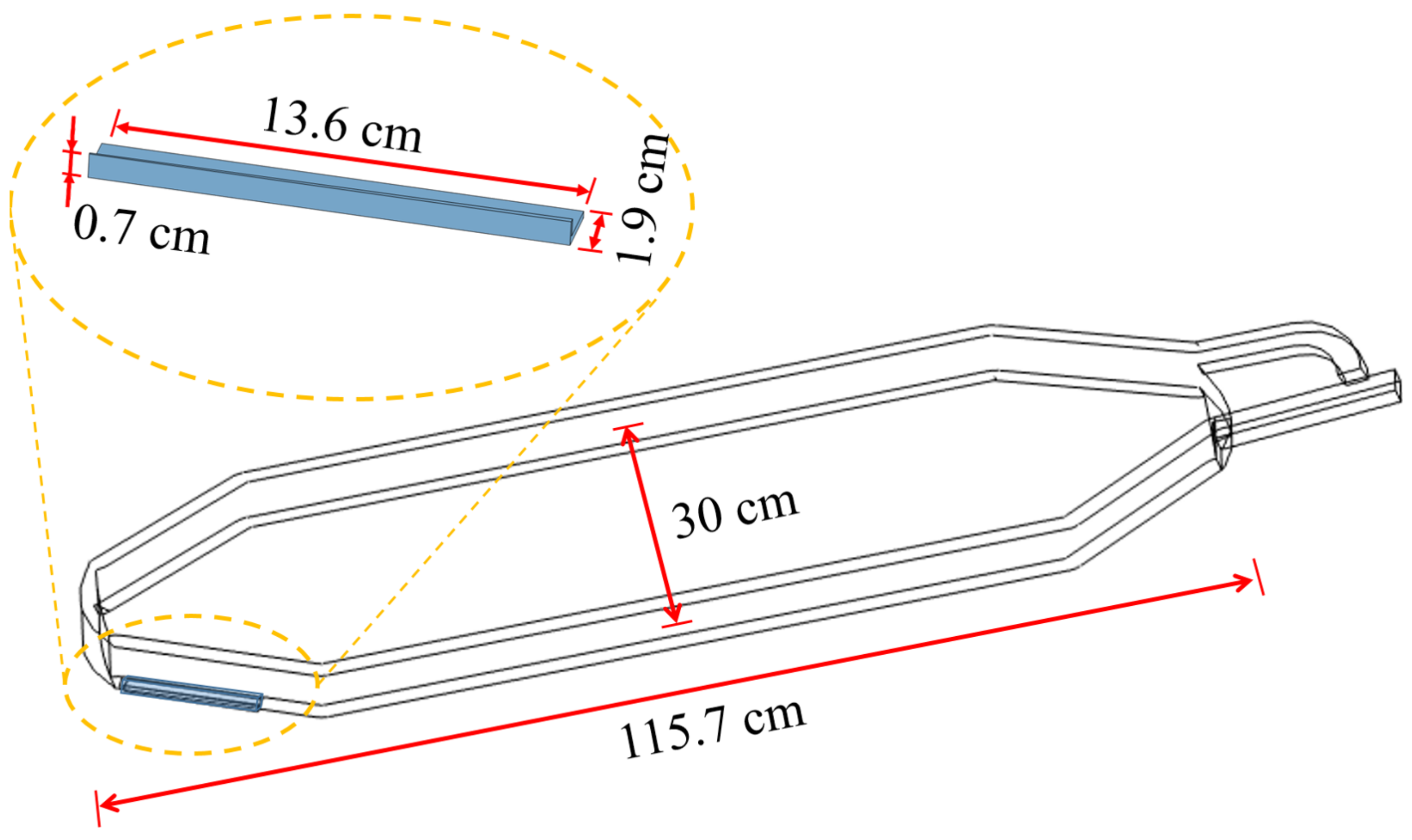
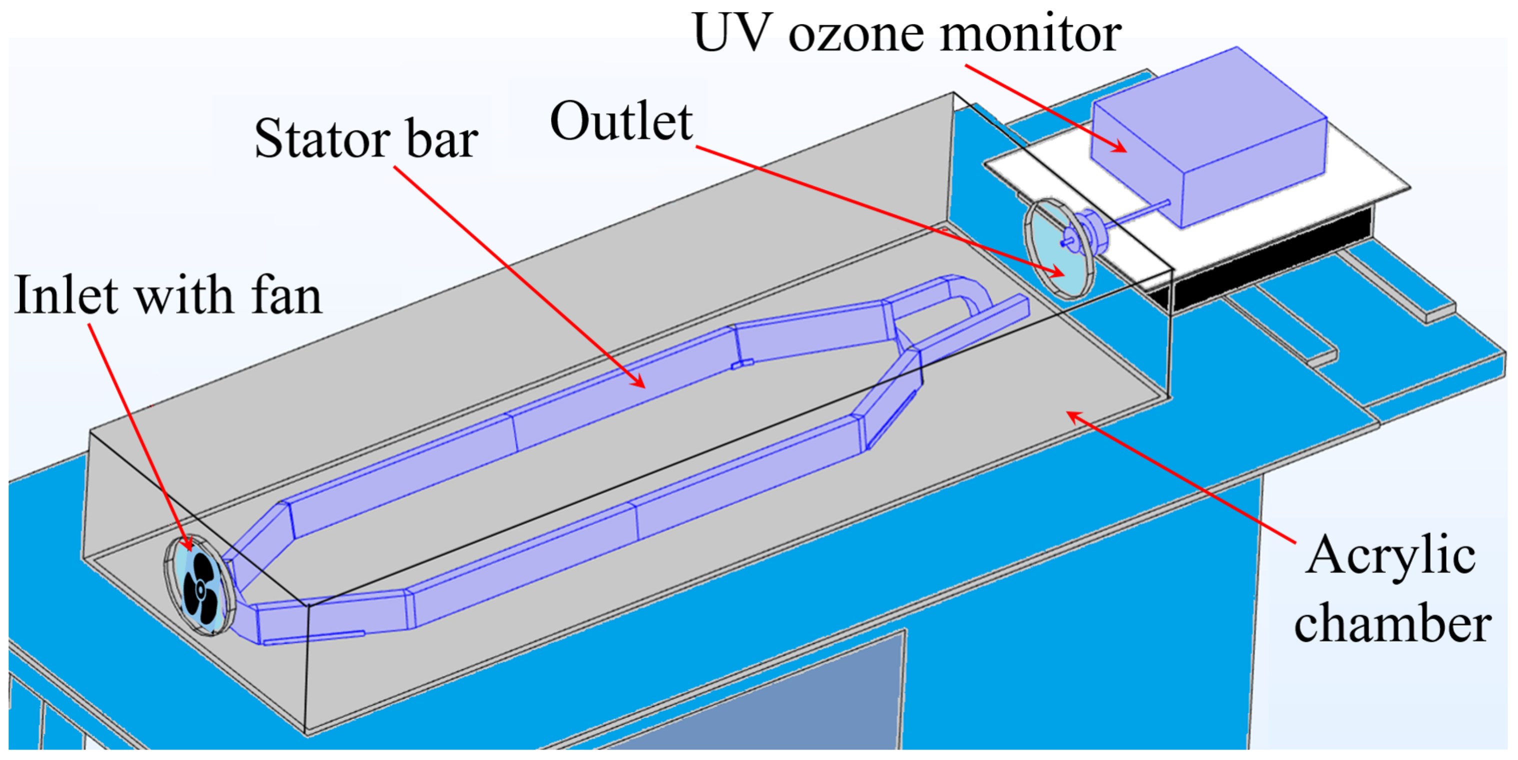
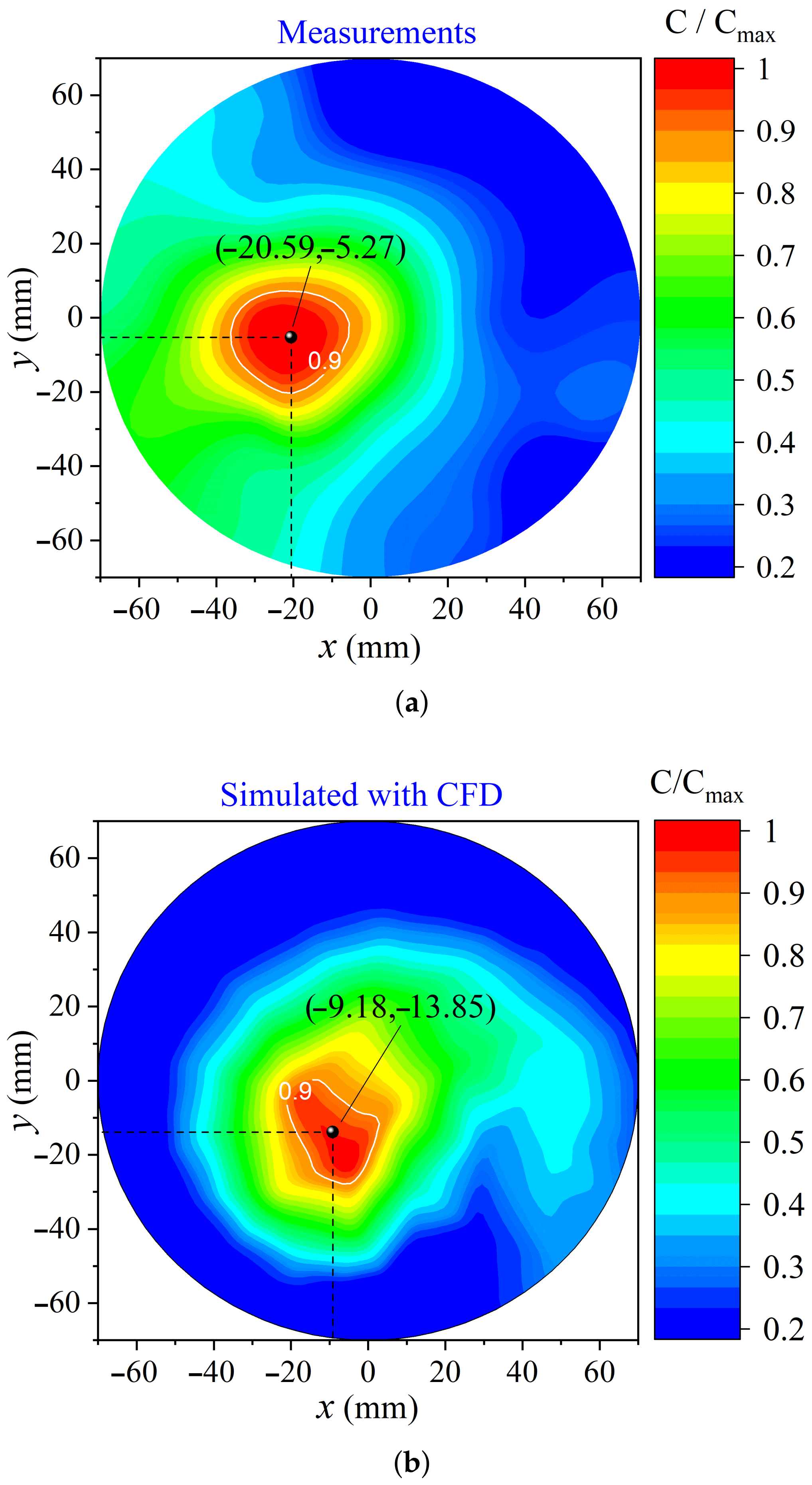
Appendix A. Validation of CFD Model Using Stator Bar Experiments

In order to check the accuracy of the CFD modeling, a stator bar with localized fault was positioned into an acrylic chamber and powered at high voltage to monitor ozone generation by partial discharges. The experiments were conducted within the high-voltage laboratory facilities of Eletronorte, a Brazilian electric power company, located in the city of Belém, Brazil. The acrylic chamber has dimensions of 145 × 21 × 50 cm3 and a circular inlet with a 14 cm fan (model Corsair AF140) attached and a free circular outlet. The inlet and outlet are located at the opposite walls of the chamber.
The bar was powered by a SERTA ET 4500 CA high voltage source. The location of the region with intensive PD emission was identified with an Ofil Systems ultraviolet camera (model Uvolle-VX), Ofil Systems, Sao Paulo, Brazil. Ozone measurements at the chamber outlet were performed with a 2B Technologies ozone monitor (model 106-L), 2B Technologies, Sao Paulo, Brazil.
Before commencement of the main experiment, initial measurements were conducted to define the presence and location of regions with PDs on the stator bar using the UV camera. Figure A1 points the identified region with the intensive PD emission, which was later set as the ozone reaction zone in the CFD model.
Figure A1. Stator bar with a localized fault. The inset highlights the identified PD emission area.
Energies 17 03173 g0a1
The stator bar was placed within the acrylic chamber as shown in Figure A2, where it was submitted to the input airflow of 1.59 m/s by the fan placed at the chamber inlet. The ozone concentration was measured at the chamber outlet. Figure A3 shows the geometric model developed for CFD simulations, which depicts the experimental setup.
Figure A2. Stator bar inside the experimental chamber.
Energies 17 03173 g0a2
Measurements of ozone concentration were fulfilled by changing the UV sensor probe position at the circular output section of the chamber, thereby creating the ozone distribution profile at the outlet plane. The 60 Hz voltage applied to the bar was 16 kV RMS. Figure A4 shows the spatial distribution of the normalized ozone concentration ( C / C m a x ) across the outlet plane, where C and C m a x are the local and the maximum values of ozone concentrations, respectively. Figure A4a shows the experimental data and Figure A4b demonstrates the simulation results obtained by the CFD model, with the indication of the coordinates where the maximum ozone concentration value occurs in each case. The coordinates of the maximum concentration were taken at the geometric center of the isoconcentration line for the relative value of 0.9, which is also shown for the measured and computed distributions in Figure A4.
Figure A3. Geometry of the CFD model of our experimental setup conceived for simulations.
Energies 17 03173 g0a3
Figure A4. Normalized ozone concentration C / C m a x at the outlet. (a) Experimental data measured with the voltage of the bar 16 kV, (b) calculated CFD results.
Energies 17 03173 g0a4
The ozone distribution at the outlet obtained by the computational model and the experimental results agree well. The peaks of ozone concentration are shifted from the center of the air outlet circle towards the lower left direction. The normalized error of the calculus can be defined as follows:
Δ = ( x c a l c x e x p ) 2 + ( y c a l c y e x p ) ) 2 / D ,
where x c a l c , y c a l c and x e x p , y e x p are respectively, calculated and experimental coordinates of the maximum point of ozone concentration, D is the diameter of the outlet where the measurements are fulfilled. In our case, the error is Δ = 0.1020 , i.e., 10%.

References

  1. Standard iec/ts 60034-27-2:2012(e); Rotating Electrical Machines—Part 27-2: Online Partial Discharge Measurements on the Stator Winding Insulation of Rotating Electrical Machines. International Organization for Standardization: Geneva, Switzerland, 2012.
  2. Dehlinger, N.; Stone, G. Surface partial discharge in hydrogenerator stator windings: Causes, symptoms, and remedies. IEEE Electr. Insul. Mag. 2020, 36, 7–18. [Google Scholar] [CrossRef]
  3. Cruz, J.S.; Fruett, F.; Lopes, R.R.; Takaki, F.L.; Tambascia, C.A.; Lima, E.R.; Giesbrecht, M. Partial Discharges Monitoring for Electric Machines Diagnosis: A Review. Energies 2022, 15, 7966. [Google Scholar] [CrossRef]
  4. Stone, G.C.; Sedding, H. Comparison of Low and High Frequency Partial Discharge Measurements on Stator Windings. In Proceedings of the Nordic Insulation Symposium, Tampere, Finland, 26 November 2019; pp. 134–138. [Google Scholar]
  5. Nair, R.P.; Vishwanath, S.B. Identification of Simultaneously Active PD Sources in Stator Insulation Using Variable Frequency Excitation. IEEE Trans. Dielectr. Electr. Insul. 2021, 28, 646–653. [Google Scholar] [CrossRef]
  6. Stone, G.C.; Sedding, H.; Veerkamp, W. What Medium and High Voltage Stator Winding Partial Discharge Testing Can-And Can Not-Tell You. In Proceedings of the 2021 IEEE IAS Petroleum and Chemical Industry Technical Conference (PCIC), San Antonio, TX, USA, 13–16 September 2021; pp. 293–302. [Google Scholar] [CrossRef]
  7. Caprara, A.; Ciotti, G.; Paschini, L. Analysis of the results of on-line Partial Discharge Monitoring and the impact of the maintenance actions on a 30 MVA synchronous generator. In Proceedings of the 2020 IEEE Electrical Insulation Conference (EIC), Knoxville, TN, USA, 22 June–3 July 2020; pp. 359–362. [Google Scholar] [CrossRef]
  8. Stone, G.C. Partial discharge diagnostics and electrical equipment insulation condition assessment. IEEE Trans. Dielectr. Electr. Insul. 2005, 12, 891–904. [Google Scholar] [CrossRef]
  9. Zhu, H.; Green, V.; Sasic, M.; Halliburton, S. Increased sensitivity of capacitive couplers for in-service PD measurement in rotating machines. IEEE Trans. Energy Convers. 1999, 14, 1184–1192. [Google Scholar] [CrossRef]
  10. Sedding, H.G.; Campbell, S.R.; Stone, G.C.; Klempner, G.S. A new sensor for detecting partial discharges in operating turbine generators. IEEE Trans. Energy Convers. 1991, 6, 700–706. [Google Scholar] [CrossRef]
  11. Stone, G.C.; Sedding, H.G.; Costello, M.J. Application of partial discharge testing to motor and generator stator winding maintenance. IEEE Trans. Ind. Appl. 1996, 32, 459–464. [Google Scholar] [CrossRef]
  12. McDermid, W.; Bromley, J.C. Experience with directional couplers for partial discharge measurements on rotating machines in operation. IEEE Trans. Energy Convers. 1999, 14, 175–184. [Google Scholar] [CrossRef]
  13. Dmitriev, V.; Oliveira, R.M.S.; Zampolo, R.F.; Vilhena, P.; Brasil, F.S.; Fernandes, M.F. Partial Discharges in Hydroelectric Generators; Springer International Publishing: Cham, Switzerland, 2023. [Google Scholar]
  14. Stone, G.C.; Culbert, I.; Boulter, E.A.; Dhirani, H. Electrical Insulation for Rotating Machines: Design, Evaluation, Aging, Testing, and Repair; Wiley-IEEE Press: Piscataway, NJ, USA, 2014; Volume 83. [Google Scholar]
  15. Buntat, Z.; Smith, I.; Mohd razali, N.A. Ozone Generation by Pulsed Streamer Discharge in Air. Appl. Phys. Res. 2009, 1, 2–10. [Google Scholar] [CrossRef]
  16. Zhu, Y.; Chen, C.; Shi, J.; Shangguan, W. A novel simulation method for predicting ozone generation in corona discharge region. Chem. Eng. Sci. 2020, 227, 115910. [Google Scholar] [CrossRef]
  17. Qin, Z.; He, Y.; Zhao, X.; Feng, Y.; Yi, X. A case analysis of turbulence characteristics and ozone perturbations over eastern China. Front. Environ. Sci. 2022, 10, 970935. [Google Scholar] [CrossRef]
  18. Langenberg, S.; Carstens, T.; Hupperich, D.; Schweighoefer, S.; Schurath, U. Technical note: Determination of binary gas-phase diffusion coefficients of unstable and adsorbing atmospheric trace gases at low temperature—Arrested flow and twin tube method. Atmos. Chem. Phys. 2020, 20, 3669–3682. [Google Scholar] [CrossRef]
  19. Ebadi Amooghin, A.; Mirrezaei, S.; Sanaeepur, H.; Moftakhari Sharifzadeh, M.M. Gas Permeation Modeling through a Multilayer Hollow Fiber Composite Membrane. J. Membr. Sci. Res. 2020, 6, 125–134. [Google Scholar] [CrossRef]
  20. Yanallah, K.; Pontiga, F.; Fernández-Rueda, A.; Castellanos, A.; Belasri, A. Ozone generation by negative corona discharge: The effect of Joule heating. J. Phys. Appl. Phys. 2008, 41, 195206. [Google Scholar] [CrossRef]
  21. Binder, E.; Draxler, A.; Muhr, M.; Pack, S.; Schwarz, R.; Egger, H.; Hummer, A. Effects of air humidity and temperature to the activities of external partial discharges of stator windings. In Proceedings of the 1999 Eleventh International Symposium on High Voltage Engineering, London, UK, 23–27 August 1999; Volume 5, pp. 264–267. [Google Scholar] [CrossRef]
  22. Petani, L.; Koker, L.; Herrmann, J.; Hagenmeyer, V.; Gengenbach, U.; Pylatiuk, C. Recent Developments in Ozone Sensor Technology for Medical Applications. Micromachines 2020, 11, 624. [Google Scholar] [CrossRef]
  23. Empowering Pumps & Equipment. Hydro Generator Refurbishment Increases Output by 15%. 2019. Available online: https://empoweringpumps.com/sulzer-hydro-generator-refurbishment-increases-output-by-15 (accessed on 19 May 2024).
  24. Oliveira, R.M.S.; Girotto, G.G.; Alcantara, L.D.S.; Lopes, N.M.; Dmitriev, V. Ozone Transport in 311 MVA Hydrogenerator: Computational Fluid Dynamics Modelling of Three-Dimensional Electric Machine. Energies 2023, 16, 8072. [Google Scholar] [CrossRef]
  25. Chung, T.J. Computational Fluid Dynamics; Cambridge University Press: Cambrige, UK, 2002. [Google Scholar]
  26. Oliveira, R.M.S.; Zampolo, R.F.; Alcantara, L.D.S.; Girotto, G.G.; Lopes, F.H.R.; Lopes, N.M.; Brasil, F.S.; Nascimento, J.A.S.; Dmitriev, V. Analysis of Ozone Production Reaction Rate and Partial Discharge Power in a Dielectric-Barrier Acrylic Chamber with 60 Hz High-Voltage Electrodes: CFD and Experimental Investigations. Energies 2023, 16, 6947. [Google Scholar] [CrossRef]
  27. Klauson, D. Physical and Chemical Properties of Ozone. 2005. Available online: https://www.eolss.net/Sample-Chapters/C07/E6-192-03.pdf (accessed on 19 May 2024).
  28. Cano-Ruiz, J.A.; Kong, D.; Balas, R.B.; Nazaroff, W.W. Removal of reactive gases at indoor surfaces: Combining mass transport and surface kinetics. Atmos. Environ. Part Gen. Top. 1993, 27, 2039–2050. [Google Scholar] [CrossRef]
  29. Williams, E.L.; Grosjean, D. Removal of atmospheric oxidants with annular denuders. Environ. Sci. Technol. 1990, 24, 811–814. [Google Scholar] [CrossRef]
  30. Simmons, A.; Colbeck, I. Resistance of various building materials to ozone deposition. Environ. Technol. 1990, 11, 973–978. [Google Scholar] [CrossRef]
  31. Mueller, F.X.; Loeb, L.; Mapes, W.H. Decomposition rates of ozone in living areas. Environ. Sci. Technol. 1973, 7, 342–346. [Google Scholar] [CrossRef] [PubMed]
  32. Cataldo, F.; Ursini, O. The Role of Carbon Nanostructures in the Ozonization of Different Carbon Black Grades, Together with Graphite and Rubber Crumb in an IR Gas Cell. Fuller. Nanotub. Carbon Nanostructures 2007, 15, 1–20. [Google Scholar] [CrossRef]
  33. Reiss, R.; Ryan, P.B.; Koutrakis, P.; Tibbetts, S.J. Ozone Reactive Chemistry on Interior Latex Paint. Environ. Sci. Technol. 1995, 29, 1906–1912. [Google Scholar] [CrossRef] [PubMed]
  34. Morrison, G.C. Ozone-Surface Interactions: Investigations of Mechanisms, Kinetics, MassTransport, and Implications for Indoor Air Quality. Ph.D. Thesis, University of California, Oakland, CA, USA, 1999. [Google Scholar]
Figure 1. (a) Photo of a real hydrogenerator [23] where the rotor is removed for maintenance; (b) the model with rotor created in this work.
Energies 17 03173 g001
Figure 2. Model of the hydrogenerator bars. (a) Several bars positioned in the stator, (b) a single bar and its dimensions.
Energies 17 03173 g002
Figure 3. (a) 3D view of the numerical model; (b) top view and the cylindrical coordinate system.
Energies 17 03173 g003aEnergies 17 03173 g003b
Figure 4. Positioning of ozone sources on the stator bars. (a) Front view and (b) top view. The yellow circles represent a single source at this height, while in the region of the green circles, three sources are positioned, varying their radial coordinate. The radial positioning of sources S 3 , S 4 , and S 5 can be seen in (a). Sources 6, 7, and 8 have different angular positions compared to those shown in (b), but the corresponding radial positions.
Energies 17 03173 g004
Figure 5. Positioning of ozone source on a stator bar in the numerical model for the radiator sector R 1 . The ozone source is highlighted in yellow, the stator bars in pink, and the rotor in blue.
Energies 17 03173 g005
Figure 6. Computational mesh generated for the generator structure; the inset shows details of the mesh in the region of stator bars.
Energies 17 03173 g006
Figure 7. Air velocity field in the radiator sector R 1 of the hydrogenerator in the horizontal plane z = 2100 mm, highlighting the regions close to the stator bars.
Energies 17 03173 g007
Figure 8. Ozone distribution on the surface of radiator: (a) R 1 for source S 1 and (b) R 2 for source S 1 ; see Figure 4a.
Energies 17 03173 g008
Figure 9. Ozone distribution on the surface of radiator: (a) R 2 for source S 2 and (b) R 1 for source S 9 ; see Figure 4a.
Energies 17 03173 g009
Figure 10. Ozone distribution on the surface of radiator: (a) R 2 for source S 10 and (b) R 1 for source S 3 ; see Figure 4a.
Energies 17 03173 g010
Figure 11. Ozone distribution on the surface of radiator: (a) R 1 for source S 4 and (b) R 1 for source S 5 ; see Figure 4a.
Energies 17 03173 g011
Figure 12. Ozone distribution on the surface of radiator: (a) R 1 for source S 8 and (b) R 1 for source S 7 ; see Figure 4a.
Energies 17 03173 g012
Figure 13. Ozone distribution on the surface of radiator: (a) R 1 for source S 6 and (b) R 2 for source S 6 ; see Figure 4a.
Energies 17 03173 g013
Table 1. Parameter γ for materials used in the model.
Material γ
Concrete 7.90 × 10 5 [30]
Stainless steel 1.80 × 10 7 [31]
Semiconductor coating layer 1.11 × 10 6 [32]
Epoxy 2.00 × 10 6 [33,34]
Table 2. Ozone source locations
Source ρ Coordinate (mm) ϕ Coordinate (Degrees)z Coordinate (mm)
S 1 3880247.54020
S 2 38802684020
S 3 3814247.52100
S 4 3871247.52100
S 5 3890247.52100
S 6 38142682100
S 7 38712682100
S 8 38902682100
S 9 3880247.5130
S 10 3880268130
Disclaimer/Publisher’s Note: The statements, opinions and data contained in all publications are solely those of the individual author(s) and contributor(s) and not of MDPI and/or the editor(s). MDPI and/or the editor(s) disclaim responsibility for any injury to people or property resulting from any ideas, methods, instructions or products referred to in the content.

