Real-Time Simulation System for Small Scale Regional Integrated Energy Systems

Abstract

Regional Integrated Energy Systems (RIESs) integrate wide spectrum of energy sources and storage with optimized energy management and further pollution reduction. This paper presents a real-time simulation system for RIESs powered by multiple digital signal processors (DSPs) with different means of data exchange. The RIES encompasses the DC microgrid (DMG), the district heat network (DHN), and the natural gas network (NGN). To realize multi-energy flow simulation, averaged switch models are investigated for different types of device-level units in the DMG, and the unified energy path method is used to build circuit-dual models of the DHN and NGN. A hierarchical island strategy (HIS) and a multi-energy dispatch strategy (MEDS) are proposed to enhance the energy flow control and operating efficiency. The two-layer HIS can adjust the operating status of device-level units in real time to achieve bus voltage stability in the DMG; MEDS uses energy conversion devices to decouple multi-energy flows and adopts the decomposed flow method to calculate the flow results for each network. The real-time simulation hardware platform is built, and both electricity-led and thermal-led experiments are carried out to verify the accuracy of models and the effectiveness of the proposed strategy. The proposed system with an energy management strategy aims to provide substantial theoretical and practical contributions to the control and simulation of RIESs, thus supporting the advancement of integrated energy systems.

1. Introduction

With the continuous growth of global energy demand and the improvement of environmental protection awareness, regional integrated energy systems (RIESs), as a key technology to achieve sustainable energy utilization, have attracted widespread attention [1,2]. RIESs leverage advanced information and communication technology, energy conversion, and optimization control technologies to establish corresponding coupling relationships among different energy subsystems, such as electricity, gas, heat, and cooling [3]. This breaks away from the traditional energy system planning and operation, which are limited to a single form of energy, and maximizes the synergy and complementary advantages of multiple forms of energy. It enhances energy utilization efficiency and the level of renewable energy integration [4].

The mainstream multi-energy flow modeling methods based on the unified model approach are primarily divided into the energy hub method and the unified energy path method [5,6]. In terms of the energy hub, Ref. [7] introduces an innovative and extended energy hub approach for the configuration optimization of RIESs, addressing the shortcomings of traditional methods by considering the combination, capacity, and operational strategy of energy devices. With the successful application of circuit theory in non-electrical energy networks, an increasing number of scholars have begun to explore the unified energy path method [8]. Ref. [9] proposes a uniform framework for modeling district heat networks (DHN) in the Laplace domain, addressing heat losses and transfer delays through an electrical-analog perspective. Ref. [10] uses a thermal circuit model for heat networks, incorporating a fractional-order model solved by a decomposition method, which enhances system flexibility and reducing operational costs.

Considering the characteristics of multi-system and multi-energy coupling in RIESs, the approaches to calculating their flow problems are mainly divided into two categories: the unified method [11] and the decomposition method [12]. Ref. [13] develops models for various energy sub-systems within an integrated electricity-gas-thermal energy system, and the multi-energy flow is calculated based on the Newton–Raphson method. Ref. [14] presents a unified time-domain model for RIES based on two-port network equivalence theory and offers a novel approach for collaborative analysis by converting complex multi-energy interactions into equivalent transfer matrices. In [15], a novel decentralized algorithm based on heterogeneous decomposition is proposed, showing effective congestion alleviation in the electric power system and efficient, robust algorithm performance with minimal communication requirements.

Modeling and simulation are fundamental to the analysis of RIESs, serving as a numerical equivalent mapping of real physical systems [6]. The dynamic simulation of RIESs considers the dynamic behavior of energy conversion equipment, typically requiring the solution of a combination of partial differential, ordinary differential, and algebraic equations. Using digital simulation technology and through collaboration between software and hardware, it ultimately achieves the simulation of multi-energy flow within the RIES [16]. The development of a software platform for joint simulation of multi-energy flow systems has been explored [17]. Ref. [18] introduces the electrical integrated energy system simulation platform SAint, developed by Pambour. Ref. Gusain et al. [19] discusses an open-source integrated energy system simulation software, EnergySim, which supports static simulations for specific systems. Based on digital simulation technology, hardware-in-the-loop (HIL) simulation incorporates real physical models, representing a form of semi-physical simulation [20]. Ref. [21] constructs a physical simulation platform for thermal networks. Utilizing similarity theory, they achieved a digital space mapping of a micro thermal network and conducted HIL simulation tests. Based on the existing literature and the state of the art on RIES simulation research, the scheduling strategies for RIESs have been investigated widely. Ref. [22] presents a distributionally robust scheduling strategy for RIESs using a two-level Stackelberg game model. In Ref. [23], a three-stage planning model for thermal energy storage is examined by a pairwise reformulation technique. Ref. [24] presents a planning model for an electricity-thermal-cooling RIES that enhances energy efficiency by integrating load clustering.

Current research on the multi-energy flow in RIES primarily targets the AC power grid [13]. However, with the growing contribution of distributed energy sources like photovoltaic and wind energy, the connection between distributed energy carriers, led by microgrids, and integrated energy systems is becoming more significant. Despite this increasing importance, there is little research focusing on the energy flow in an RIES that incorporates a microgrid. DC microgrids (DMGs) offer simplified operation coordination, as the DC bus voltage is the sole control parameter, eliminating the frequency and reactive power challenges inherent in AC systems [25]. Regarding the optimal dispatch of microgrids, Ref. [26] utilizes a two-level hierarchical multi-agent system for microgrids to achieve significant cost reductions by optimally dispatching power among microgrid components. Ref. [27] introduces a real-time distributed economic dispatch scheme for grid-connected microgrids, employing a virtual leader agent for power balance and a consensus algorithm for optimization. The above literature mainly considers the optimal dispatch of microgrids from the perspective of cost minimization, and does not consider the actual dynamic behavior of each module in the microgrid. So far, few studies have conducted dynamic behavior simulation analysis from the perspective of component models, simulation conditions, and control complexity (including communication delay and security) of microgrids [23]. To bridge these identified research gaps, this paper sets out to address crucial issues in DMG control, together with the energy flow calculation of DHN and natural gas networks (NGNs). Our approach involves developing and validating new control strategies and schedule algorithms. DMG employs an improved two-layer hierarchical control system which contains bus and device control layer, requiring only the collection of each device’s output current and bus voltage. The multi-energy flow scheduling strategy focuses on the coupling nodes between networks as breakthrough points and uses the decomposition method for power flow calculation. By leveraging the real-time capabilities of a hardware simulation platform, we aim to propel the simulation of RIESs towards enhanced efficiency, reliability, and sustainability. The main contributions of this paper are as follows:

• Modeling and control of device-level units and energy networks: Averaged switch models of device-level units in DMG are developed and verified in PSIM; the unified energy path method is utilized in both DHNs and NGNs. These models and methods provide new perspectives for understanding and calculating complex energy systems.
• Development of energy control algorithms: Hierarchical control strategies for DMG island operation mode and multi-energy dispatch strategies are designed for RIES. These strategies and algorithms can effectively calculate the energy flow and ensure stable operation of the RIES.
• DSP-based real-time simulation platform design: A novel simulation platform is built, using DSP as the core processing unit to support highly complex system model iteration and data communication. Through this platform, real-time simulation results of the mathematical models and proposed control algorithms can be achieved.

The organization of this paper is as follows: Section 2 describes the mathematical models of device-level units in RIESs; the unified modeling of DHN and NGN is documented in Section 3; Section 4 introduces the hierarchical island strategy (HIS) for DMG and the multi-energy dispatch strategy (MEDS) for RIESs; a real-time simulation platform for RIESs is constructed and experiments verification are conducted in Section 5.

2. Device-Level Unit Modeling

2.1. Photovoltaic Generation Unit

The photovoltaic (PV) panels are connected to the DC bus through boost converter [28]. The circuit topology is shown in Figure 1, where T and S are the light intensity and temperature; $C_p$ and $L_1$ are the capacitor and inductor at low-voltage side; $C_1$ is the output voltage capacitor; $L_{g1}$ and $r_{g1}$ are the equivalent inductance and resistance of transmission lines. The averaged switch model of the boost circuit is obtained as follows:

$$\left\{\begin{array}{cc}\hfill C_p\frac{\mathrm{d}{〈v_{pv}〉}_{T_s}}{\mathrm{d}t}& ={〈i_{pv}〉}_{T_s}-{〈i_{L_1}〉}_{T_s}\hfill \\ \hfill L_1\frac{\mathrm{d}{〈i_{L_1}〉}_{T_s}}{\mathrm{d}t}& ={〈v_{pv}〉}_{T_s}-(1-d)·{〈v_{C_1}〉}_{T_s}\hfill \\ \hfill C_1\frac{\mathrm{d}{〈v_{C_1}〉}_{T_s}}{\mathrm{d}t}& =(1-d){〈i_{L_1}〉}_{T_s}-{〈i_{pg}〉}_{T_s}\hfill \\ \hfill L_{g_1}\frac{\mathrm{d}{〈i_{pg}〉}_{T_s}}{\mathrm{d}t}& ={〈v_{C_1}〉}_{T_s}-{〈v_{n1}〉}_{T_s}-r_{g_1}{〈i_{pg}〉}_{T_s}\hfill \end{array}\right.$$

(1)

where $v_{pv}$ and $i_{pv}$ are the output voltage and current of the photovoltaic panel; $i_{L1}$ is the current of the inductor $L_1$; $v_{C1}$ is the converter output voltage; $i_{pg}$ and $v_{n1}$ are the output current and node voltage of the PV generation unit.

2.2. Micro Turbine Generation Unit

This paper uses the single-shaft micro turbine (MT) model proposed by Rowen as the object of dynamic modeling [29], and studies the electromechanical characteristics of the MT power generation system on its basis. MT operates coaxially with the isotropic permanent magnet synchronous generator (PMSG), then connected to DMG via three-phase voltage source rectifier (VSR) The electromagnetic torque and motion equation can be expressed as [30]:

$$T_e=\frac{3}{2}{p}_n{\psi }_f{i}_q$$

(2)

$$J\frac{\mathrm{d}{\omega }_m}{\mathrm{d}t}=T_m-T_e-D{\omega }_m$$

(3)

where $T_e$ and ${\Phi }_f$, respectively, denote the electromagnetic torque and the flux linkage of the PMSG; $i_q$ is the q-axis component of PMSG current; $T_m$ is the mechanical torque output from the MT; D and J are the friction coefficient and moment of inertia; ${\omega }_m$ and $p_n$ represent the mechanical angular velocity and the number of pole pairs, with their relationship to the electrical angular velocity ${\omega }_e$ being: ${\omega }_e=p_n{\omega }_m$.

Figure 2 shows the circuit topology of the PMSG-VSR circuit, where $e_{sa}$, $e_{sb}$, and $e_{sc}$ are the induced electromotive forces of the PMSG; $i_{sa}$, $i_{sb}$, and $i_{sc}$ represent the three-phase stator currents; $u_a$, $u_b$, and $u_c$ are the phase voltages; $R_s$ and $L_s$ denote the stator resistor and inductor, and $C_{dc}$ is the DC output capacitor. $L_{g2}$ and $r_{g2}$, respectively, represent the equivalent inductance and resistance of the transmission line.

Establish the PMSG-VSR averaged switch model under d-q coordinates:

$$\left\{\begin{array}{c}{L}_{sd}\frac{\mathrm{d}{〈i_{sd}〉}_{T_s}}{\mathrm{d}t}=-R_s{〈i_{sd}〉}_{T_s}+{\omega }_e{L}_{sq}{〈i_{sq}〉}_{T_s}-{〈u_d〉}_{T_s}\hfill \\ L_{sq}\frac{\mathrm{d}{〈i_{sq}〉}_{T_s}}{\mathrm{d}t}=-R_s{〈i_{sq}〉}_{T_s}+{\omega }_e{L}_{sd}{〈i_{sd}〉}_{T_s}-{〈u_q〉}_{T_s}+{\omega }_e{\psi }_f\hfill \\ C_{dc}\frac{\mathrm{d}{〈v_{dc}〉}_{T_s}}{\mathrm{d}t}=\frac{3}{2}(d_d{〈i_{sd}〉}_{T_s}+d_q{〈i_{sq}〉}_{T_s})-{〈i_{MT}〉}_{T_s}\hfill \\ L_{g_2}\frac{\mathrm{d}{〈i_{MT}〉}_{T_s}}{\mathrm{d}t}=\mathrm{d}{〈v_{dc}〉}_{T_s}-{〈i_{MT}〉}_{T_s}·r_{g_2}-{〈v_{n2}〉}_{T_s}\hfill \end{array}\right.$$

(4)

where, $i_{sd}$ and $i_{sq}$ are the d-q components of stator currents; $u_d$ and $u_q$ are the d-q components of phase voltages; $L_{sd}$ and $L_{sq}$ are the d-q components of stator inductor; $i_{MT}$ and $v_{n2}$ represent the output current and node voltage of the MT generation unit.

If losses are ignored, the electromagnetic power $P_{em}$ and the direct current power $P_{dc}$ should be balanced:

$$\begin{array}{cc}\hfill & P_{em}=T_e{\omega }_e=\frac{3}{2}{\psi }_f{i}_{sq}·{\omega }_e\hfill \end{array}$$

(5)

$$\begin{array}{cc}\hfill & P_{dc}=v_{dc}{i}_{dc}=v_{dc}\left(C_{dc}\frac{\mathrm{d}{v}_{dc}}{\mathrm{d}t}+i_{MT}\right)\hfill \end{array}$$

(6)

The q-axis current can be represented as:

$$i_{sq}=\frac{2v_{dc}}{3{\omega }_e{\psi }_f}\left(C_{dc}\frac{\mathrm{d}{v}_{dc}}{\mathrm{d}t}+i_{MT}\right)$$

(7)

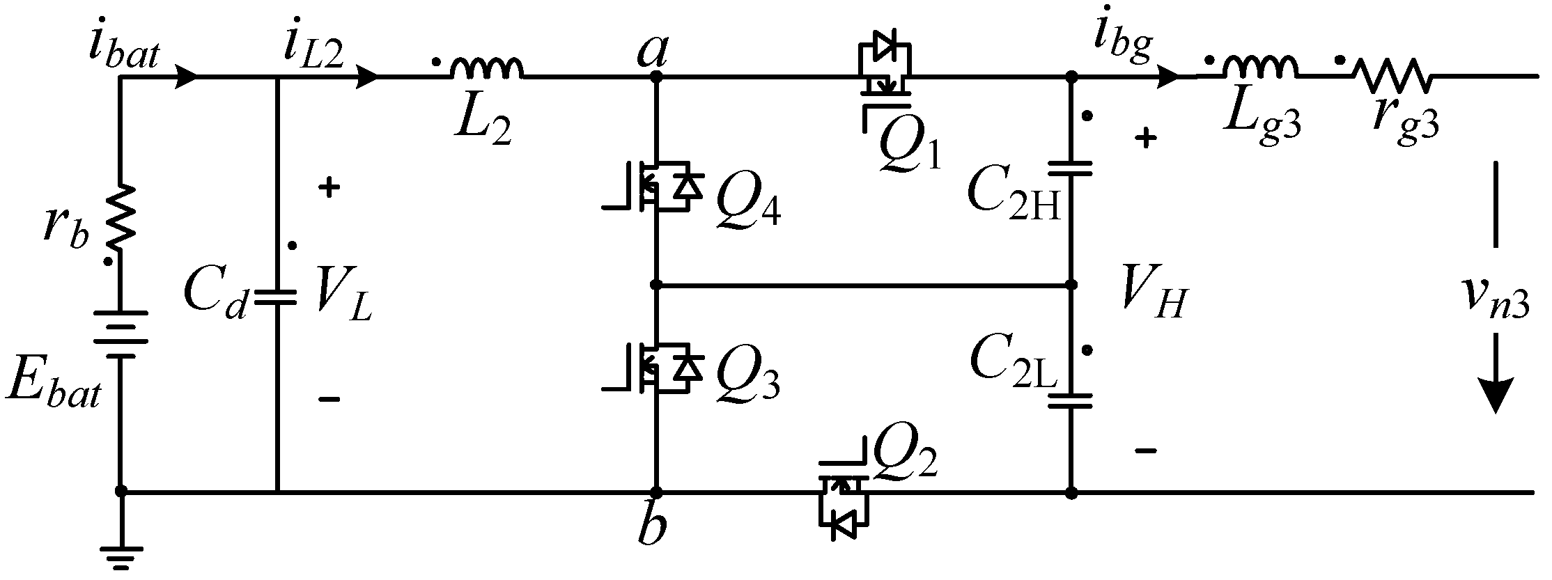
2.3. Energy Storage Unit

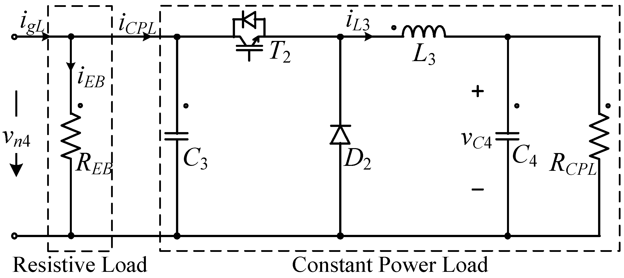
Considering the characteristics of bidirectional energy flow in the energy storage unit within a DMG, and in order to improve energy conversion efficiency and reduce the voltage stress on switch tubes, this paper adopts battery (BAT) for the energy storage entity. The circuit topology selected is a non-isolated three-level (TL) buck–boost bidirectional converter. Its typical topology is shown in Figure 3, where $E_{bat}$ and $r_b$ represent the battery voltage and internal resistance; $C_{2H}$ and $C_{2L}$ are the support capacitors on the high voltage side; $C_d$ and $L_2$ are the filtering capacitor and inductor on the low voltage side; $L_{g3}$ and $r_{g3}$ are the equivalent inductance and resistance of the transmission line.

When the DMG has surplus power, the energy storage unit charges. Taking duty ratio $>0.5$ as an example for modeling, the averaged switch model under buck operation is obtained:

$$\left\{\begin{array}{c}{〈v_L〉}_{T_s}=E_{bat}+{〈i_{bat}〉}_{T_s}·r_b\hfill \\ L_2\frac{\mathrm{d}{〈i_{L_2}〉}_{T_s}}{\mathrm{d}t}=d·{〈v_H〉}_{T_s}-{〈v_L〉}_{T_s}\hfill \\ C_d\frac{\mathrm{d}{〈v_L〉}_{T_s}}{\mathrm{d}t}={〈i_{L_2}〉}_{T_s}-{〈i_{bat}〉}_{T_s}\hfill \\ \frac{C_{2H}}{2}\frac{\mathrm{d}{〈v_H〉}_{T_s}}{\mathrm{d}t}=d·{〈i_{bg}〉}_{T_s}-{〈i_{L_2}〉}_{T_s}\hfill \\ L_{g_3}\frac{\mathrm{d}{〈i_{bg}〉}_{T_s}}{\mathrm{d}t}={〈v_{n3}〉}_{T_s}-{〈i_{bg}〉}_{T_s}·r_{g_3}-{〈v_H〉}_{T_s}\hfill \end{array}\right.$$

(8)

When the load demand in DMG is higher than generation, the energy storage unit kicks in. Taking duty ratio $<0.5$ as an example for modeling, the average switching model under boost operation is obtained:

$$\left\{\begin{array}{c}{〈v_L〉}_{T_s}=E_{bat}-{〈i_{bat}〉}_{T_s}·r_b\hfill \\ L_2\frac{\mathrm{d}{〈i_{L_2}〉}_{T_s}}{\mathrm{d}t}={〈v_L〉}_{T_s}-(1-d)·{〈v_H〉}_{T_s}\hfill \\ C_d\frac{\mathrm{d}{〈v_L〉}_{T_s}}{\mathrm{d}t}={〈i_{bat}〉}_{T_s}-{〈i_{L_2}〉}_{T_s}\hfill \\ \frac{C_{2H}}{2}\frac{\mathrm{d}{〈v_H〉}_{T_s}}{\mathrm{d}t}=(1-d)·{〈i_{L_2}〉}_{T_s}-{〈i_{bg}〉}_{T_s}\hfill \\ L_{g_3}\frac{\mathrm{d}{〈i_{bg}〉}_{T_s}}{\mathrm{d}t}={〈v_H〉}_{T_s}-{〈i_{bg}〉}_{T_s}·r_{g_3}-{〈v_{n3}〉}_{T_s}\hfill \end{array}\right.$$

(9)

In Equations (8) and (9), $V_L$ is the low side voltage of the converter; $V_H$ is the high side voltage of the converter; $i_{L_2}$ is the current flowing through the inductor $L_2$; $i_{bg}$ and $v_{n3}$ are the output current and node voltage of the energy storage unit.

The state of charge (SOC) of the battery is defined as:

$$SOC=\frac{Q-\int i_{bat}{T}_s}{Q}$$

(10)

where $i_{bat}$ is the battery charging/discharging current; $T_s$ is the current sampling time, and Q is the battery capacity.

To guarantee the BAT storage long service time while meeting the DMG power demand, it is required that the SOC remains within a certain range, which is

$$SO{C}_{\min }\le SOC\le SO{C}_{\max }$$

(11)

2.4. Load Unit

The load unit consists of resistive loads represented by electric boilers (EB) and Constant Power Loads (CPL), as shown in Figure 4. In the figure, the resistive load is composed of a single resistor $R_{EB}$, whose power consumption varies with voltage and its own resistance value; CPL is implemented internally through a buck circuit. $C_3$ and $C_4$ are the voltage stabilizing capacitors, with $R_{CPL}$ being the load resistance of the buck circuit.

The averaged switch model of the load unit is obtained as follows:

$$\left\{\begin{array}{c}{C}_3\frac{\mathrm{d}{〈v_{bus}〉}_{T_s}}{\mathrm{d}t}={〈i_{CPL}〉}_{T_s}-d·{〈i_{L_3}〉}_{T_s}\hfill \\ L_3\frac{\mathrm{d}{〈i_{L_3}〉}_{T_s}}{\mathrm{d}t}=d·{〈v_{n4}〉}_{T_s}-{〈v_{C_4}〉}_{T_s}\hfill \\ C_4\frac{\mathrm{d}{〈v_{C_4}〉}_{T_s}}{\mathrm{d}t}={〈i_{L_3}〉}_{T_s}-\frac{{〈v_{C_4}〉}_{T_s}}{R_{CPL}}\hfill \\ {〈i_{gL}〉}_{T_s}={〈i_{EB}〉}_{T_s}+{〈i_{CPL}〉}_{T_s}\hfill \end{array}\right.$$

(12)

where $i_{gL}$ and $v_{n4}$, respectively, represent the input current and node voltage of the load unit; $i_{L_3}$ is the inductor current; $v_{C_4}$ is the output voltage of the buck converter.

3. Energy Networks Modeling

Operating control of RIES is based on the modeling and analysis of various energy networks. While the electrical network has developed a relatively mature circuit theory foundation based on the simplification from “field” to “path”, this section establishes circuit-dual models for DHNs and NGNs based on Ref. [31]. Node-loop equations are to be established, steady-state energy flow of the gas–heat network will be solved through an iterative correction method.

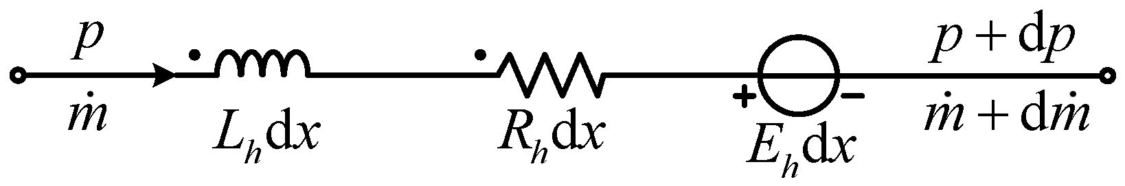
3.1. District Heat Network

3.1.1. Model Establishment

The analysis of DHNs mainly includes hydraulic analysis and thermal analysis. Under a control-by-temperature mode, there is a unidirectional coupling relationship between the hydraulic process and the thermal process, meaning the hydraulic process can affect the thermal process, but the thermal process does not influence the hydraulic process.

The flow of water in pipes can be described by the mass conservation equation and momentum conservation equation, obtaining a distributed parameter hydraulic model as follows [31]:

$$\begin{array}{cc}\hfill & \frac{\partial \dot{m}}{\partial x}=0\hfill \\ \hfill \frac{\partial p}{\partial x}=-\frac{1}{A}\frac{\partial \dot{m}}{\partial t}& -\frac{C_D{\dot{m}}_0}{\rho AD}\dot{m}+\frac{C_D{\dot{m}}_0^2}{2\rho AD}+\rho g\hfill \end{array}$$

(13)

where $\rho$, $\dot{m}$, and p represent the density, mass flow rate, and pressure of water; D, $C_D$, and A are the pipe’s inner diameter, resistance coefficient, and cross-sectional area of the pipe; g, t, and x are the gravitational acceleration, time, and space; ${\dot{m}}_0$ is the base value of the mass flow rate.

Analogizing Equation (13) to a circuit, where water pressure p is analogous to voltage, and mass flow rate $\dot{m}$ is analogous to current [8], abstracts water circuit elements such as water resistor $R_h$, water inductor $L_h$, and water pressure source $E_h$, as shown in Equation (14). Thus, the distributed parameter equivalent circuit model of a hydraulic branch is shown in Figure 5.

$$R_h=\frac{C_D{\dot{m}}_0}{\rho AD};L_h=\frac{1}{A};E_h=\rho g+\frac{C_D{\dot{m}}_0^2}{2\rho AD}$$

(14)

Besides pipelines, for flow control valves with a given opening $k_v$ and booster pumps with a given rotation frequency ${\omega }_p$, the models after incremental approximation of the square terms are shown in Equations (15) and (16), respectively. They can be represented by the equivalent circuit model shown in Figure 6.

$$\Delta p_{valve}=k_v{\dot{m}}^2\approx 2k_v{\dot{m}}_0·\dot{m}-k_v{\dot{m}}_0^2$$

(15)

$$\begin{array}{cc}\hfill & \Delta p_{pump}=k_{p1}{\dot{m}}^2+k_{p2}{\omega }_p\dot{m}+k_{p3}{\omega }_p^2\hfill \\ \hfill & \approx (2k_{p1}{\dot{m}}_0+k_{p2}{\omega }_p)\dot{m}+(k_{p3}{\omega }_p^2-k_{p1}{\dot{m}}_0^2)\hfill \end{array}$$

(16)

where $k_{p1}$, $k_{p2}$, and $k_{p3}$ are inherent coefficients related to the booster pump.

The first-order transport model for thermal flow in pipes is shown as follows [9]:

$$c\rho A\frac{\partial T}{\partial t}+c\dot{m}\frac{\partial T}{\partial x}+\lambda T=0$$

(17)

where c and T, respectively, represent the specific heat capacity of water and the relative temperature between the water temperature and the ambient temperature; temperature loss is represented as the product of the heat loss coefficient $\lambda$ and temperature T.

The effective thermal energy transferred in the pipeline above ground temperature is defined as the thermal power of the water flow [8]:

$$\Phi =c\dot{m}T$$

(18)

Substituting into Equation (17) is rewritten as follows:

$$\begin{array}{cc}\hfill \frac{\partial \Phi }{\partial x}& =-c\rho A\frac{\partial T}{\partial t}-\lambda T\hfill \\ \hfill \frac{\partial T}{\partial x}& =-\frac{\rho A}{c{\dot{m}}^2}\frac{\partial \Phi }{\partial t}-\frac{\lambda }{c^2{\dot{m}}^2}\Phi \hfill \end{array}$$

(19)

Analogizing Equation (19) to a circuit, where temperature T is analogous to voltage, and thermal power $\Phi$ is analogous to current, abstracts thermal circuit elements such as thermal resistor $R_t$, thermal inductor $L_t$, thermal conductor $g_t$, thermal capacitor $C_t$ as shown in Equation (20). Thus, the distributed parameter equivalent circuit model of a thermal branch is shown in Figure 7.

$$R_t=\frac{\lambda }{c^2{m}^2};L_t=\frac{\rho A}{c{m}^2};g_t=\lambda ;C_t=c\rho A$$

(20)

3.1.2. Node-Loop Equations

In circuit theory, Kirchhoff’s laws describe the linear algebraic relationships between branch currents and voltages (corresponding to the mass flow and water pressure in hydraulic branches). Thus, by analogy, the node flow balance and loop pressure balance rules in hydraulics can be derived as [8]:

$${\mathbf{A}}_h{\dot{\mathbf{m}}}_b={\dot{\mathbf{m}}}_n$$

(21)

$${\mathbf{A}}_h^{\mathrm{T}}{\mathbf{p}}_n={\mathbf{p}}_b$$

(22)

Here, ${\mathbf{A}}_h$ is the hydraulic node-branch incidence matrix; ${\dot{\mathbf{m}}}_b$ and ${\mathbf{p}}_b$ are the column vectors consisting of branch mass flow rates and water pressures, respectively; ${\dot{\mathbf{m}}}_n$ and ${\mathbf{p}}_n$ are the column vectors consisting of node mass flow rates and water pressures, respectively.

The thermal network shares the same node-branch incidence matrix ${\mathbf{A}}_h$ with the hydraulic network, and the thermal network’s nodes involve merging and diverging flows. Its equations are as follows [31]:

$${\mathbf{T}}_{node}={\overline{\mathbf{A}}}_{h-}{\mathbf{T}}_l+{\mathbf{T}}_n$$

(23)

$${\mathbf{T}}_s={\mathbf{A}}_{h+}^{\mathrm{T}}{\mathbf{T}}_{node}$$

(24)

Here, ${\mathbf{T}}_s$ and ${\mathbf{T}}_l$ are the column vectors consisting of the temperatures at the two ends of each pipeline, respectively; ${\mathbf{T}}_{node}$ is the column vector consisting of the temperatures at each node; ${\mathbf{T}}_n$ is the column vector consisting of injected temperatures at each node; ${\mathbf{A}}_{h+}$ is the node-outflow branch matrix; ${\overline{\mathbf{A}}}_{h-}$ is the weighted node-inflow branch matrix.

3.2. Natural Gas Network

3.2.1. Model Establishment

The one-dimensional flow equation of natural gas in pipelines is similar to the hydraulic model, with its distributed parameter gas network model equation given by [8]:

$$\begin{array}{cc}\hfill \frac{\partial G}{\partial x}=& -\frac{A_g}{R{T}_g}·\frac{\partial p_g}{\partial t}\hfill \\ \hfill \frac{\partial p_g}{\partial x}=-\frac{1}{A_g}·\frac{\partial G}{\partial t}& -\frac{f{v}_{g_0}}{D_g}G+\frac{A_{g}f·v_{g_0}^2}{2R{T}_g{D}_g}{p}_g\hfill \end{array}$$

(25)

R and $T_g$ are the gas constant and temperature of natural gas; G and $p_g$ represent the mass flow rate of natural gas branches and node gas pressure; $D_g$, $A_g$, and f, respectively, are the inner diameter, cross-sectional area, and friction coefficient of the natural gas pipeline; $v_{g_0}$ is the base value of natural gas flow velocity.

Analogizing Equation (25) to a circuit, where pressure $p_g$ is analogous to voltage, and mass flow rate G is analogous to current, gas circuit elements such as gas resistor $R_g$, gas inductor $L_g$, gas capacitor $C_g$, controlled gas pressure source $k_g$ are obtained by Equation (26). The distributed parameter equivalent circuit model of a gaseous branch is shown in Figure 8.

$$\begin{array}{ccc}\hfill R_g=\frac{f{v}_{g_0}}{D_g}& ,L_g=\frac{1}{A_g},C_g=\frac{A_g}{R{T}_g},k_g\hfill & \hfill =\frac{A_g{v}_{g_0}^{2}f·p_g}{2R{T}_g{D}_g}\end{array}$$

(26)

3.2.2. Node-Loop Equations

Kirchhoff’s laws are also applicable to the branches of NGNs, leading to the derivation of node flow balance and loop pressure balance equations for the gas network as follows [8]:

$$\begin{array}{cc}\hfill {\mathbf{A}}_g{\mathbf{G}}_b& ={\mathbf{G}}_n\hfill \end{array}$$

(27)

$$\begin{array}{cc}\hfill {\mathbf{A}}_{g+}^T{\mathbf{p}}_n& ={\mathbf{p}}_s\hfill \end{array}$$

(28)

In these equations, ${\mathbf{A}}_g$ and ${\mathbf{A}}_{g+}$ represent the node-branch incidence matrix and the node-outflow branch matrix of the NGN, respectively; ${\mathbf{G}}_n$ is the column vector composed of mass flows injected at the nodes; ${\mathbf{G}}_b$ is the column vector composed of branch mass flows; and ${\mathbf{p}}_s$ is the column vector composed of pressures at the start of each branch.

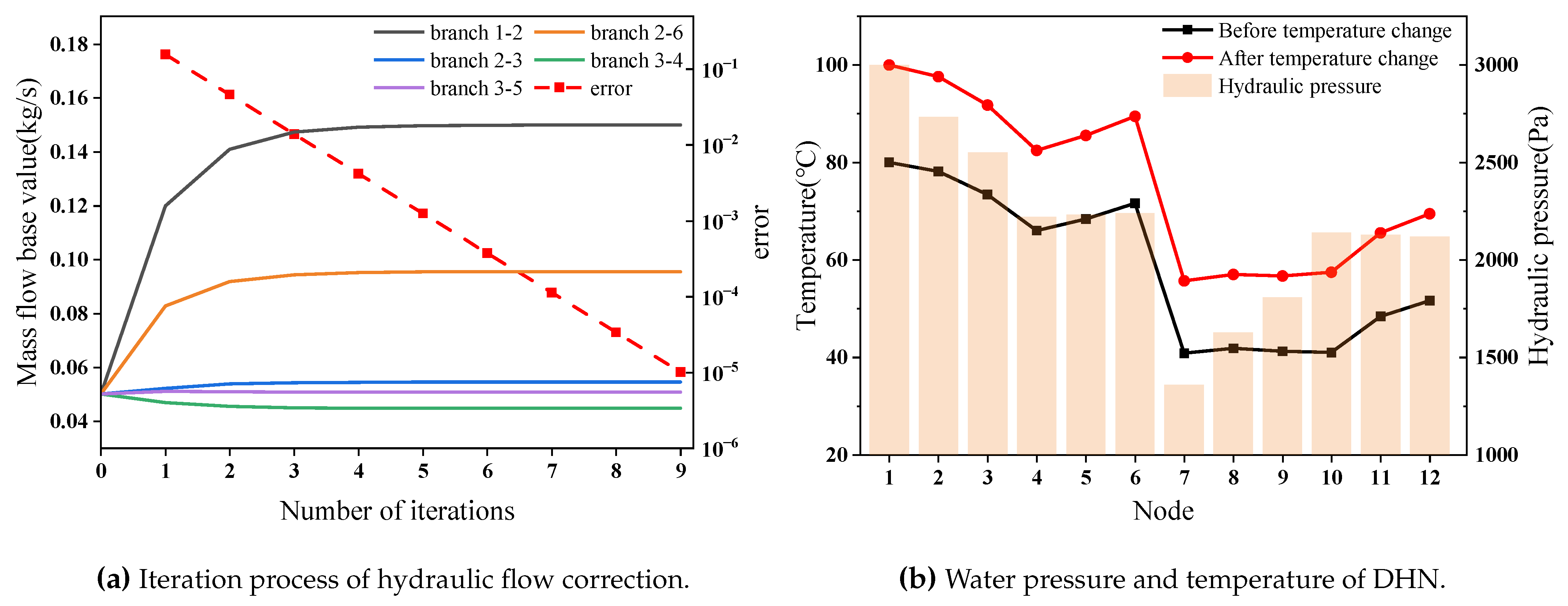
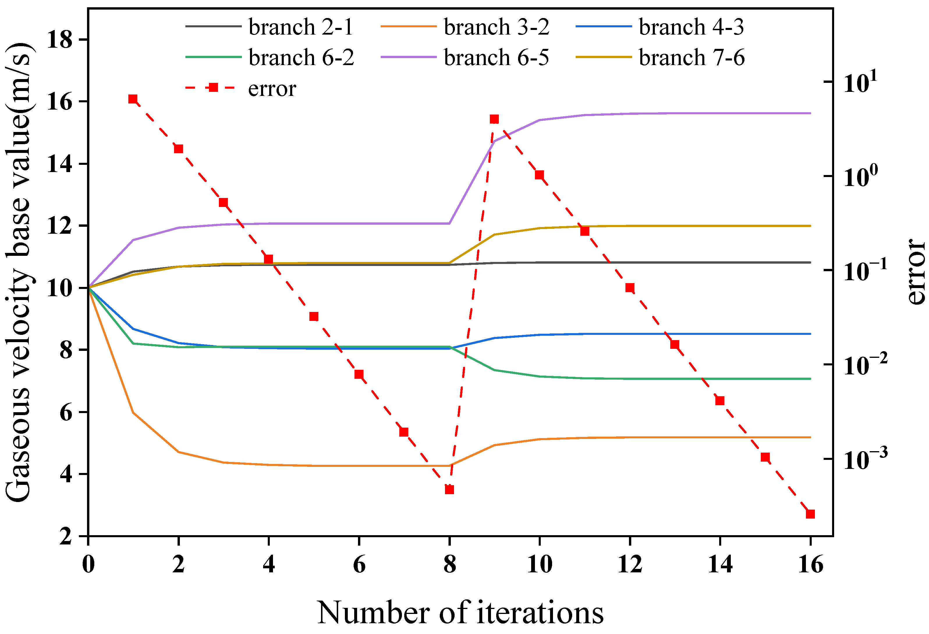
3.3. Steady-State Energy Flow Correction

In this paper, the square terms are approximated by using the Taylor series for incremental approximation [9]. This approximation method requires the adjustment of the base value through numerical iterative methods, reducing deviations from the actual values, thereby correcting errors in the steady-state flow. The detailed correction process is as follows:

(1)

Initially specify the branch mass flow or velocity base value $x_0\left[k\right]$.

(2)

Update the hydraulic or gas matrix equation, then conduct the hydraulic and gaseous steady-state flow calculation, obtaining the actual branch mass flow value $\widehat{x}\left[k\right]$.

(3)

Calculate the distance between the branch mass flow base value $x_0\left[k\right]$ and the actual value $\widehat{x}\left[k\right]$: If $∥\widehat{x}\left[k\right]-x_0\left[k\right]∥\le \epsilon$ (where $\epsilon$ is a predefined convergence threshold), the accuracy requirements are met, and the iteration ends. Otherwise, update the branch mass flow or velocity base value according to Equation (29) and return to step (2).

$$\begin{array}{c}\hfill x_0[k+1]=(1-\mu )x_0\left[k\right]+\mu \widehat{x}\left[k\right];\end{array}$$

(29)

Here, $\mu$ is the step size for updating the base value.

4. RIES Operation Control Strategies

4.1. Hierarchical Island Strategy

The island operation of a DMG refers to the independent operation without connection to the AC distribution network, where each distributed energy resource and storage device within the system supplies power to the load [32]. Under this operational state, it is necessary to ensure a real-time balance between the output power and the load demand within the system, while also maintaining the DC bus voltage stable. In order to address the coordinated control between device-level units, this paper proposes a novel hierarchical island control strategy, based on the equivalent method of node voltage and current, controls the DMG from the device layer and bus layer [33,34].

4.1.1. Device Control Layer

The structure of the DMG discussed in this paper mainly includes a PV generation unit, a BAT storage unit and load unit, an MT generation unit, and related power electronics devices. The control block diagram of the device level units is shown in Figure 9. The red boxes are the unit transfer functions, which can be obtained from the averaged switch model in Section 2 through small signal analysis and Laplace transform.

The DC grid backbone is modeled as a DC voltage source $v_{\mathrm{bus}}$ in series with a resistor $r_{\mathrm{bus}}$, paralleled by a bus voltage-stabilizing capacitor $C_{\mathrm{bus}}$. Each device-level unit is equivalently represented by a controlled current source in current mode, resulting in the equivalent circuit structure of the islanded DMG as shown in Figure 10. $Z_L$ represents the line impedance, and applying the node voltage method yields:

$$\left[\begin{array}{cccc}\frac{2}{Z_L}& \frac{-1}{Z_L}& 0& 0\\ \frac{-1}{Z_L}& \frac{2}{Z_L}& \frac{-1}{Z_L}& 0\\ 0& \frac{-1}{Z_L}& \frac{1}{Z_L}& 0\\ 0& 0& \frac{-1}{Z_L}& \frac{1}{Z_L}\end{array}\right]\left[\begin{array}{c}{v}_{n1}\\ v_{n2}\\ v_{n3}\\ v_{n4}\end{array}\right]=\left[\begin{array}{c}{i}_{\mathrm{bus}}+i_{\mathrm{pg}}\\ i_{\mathrm{MT}}\\ i_{\mathrm{bg}}-i_{\mathrm{gL}}\\ -i_{\mathrm{gL}}\end{array}\right]$$

(30)

The supplementary equations are

$$\begin{array}{cc}\hfill & C_{\mathrm{bus}}\frac{\mathrm{d}{v}_{\mathrm{bus}}}{\mathrm{d}t}=i_{bus}-\frac{v_{\mathrm{bus}}-v_{n1}}{Z_L}\hfill \\ \hfill & i_{\mathrm{bus}}=(E_{\mathrm{bus}}-v_{\mathrm{bus}})/r_{\mathrm{bus}}\hfill \end{array}$$

(31)

From Equations (30) and (31), the node voltages of each device-level unit, as well as the DC bus voltage and current, can be calculated.

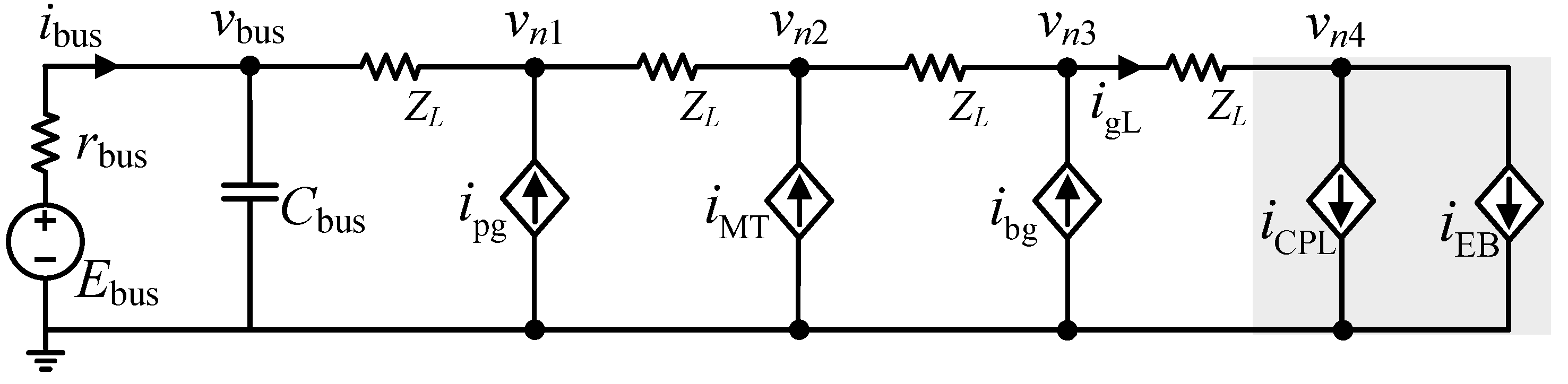
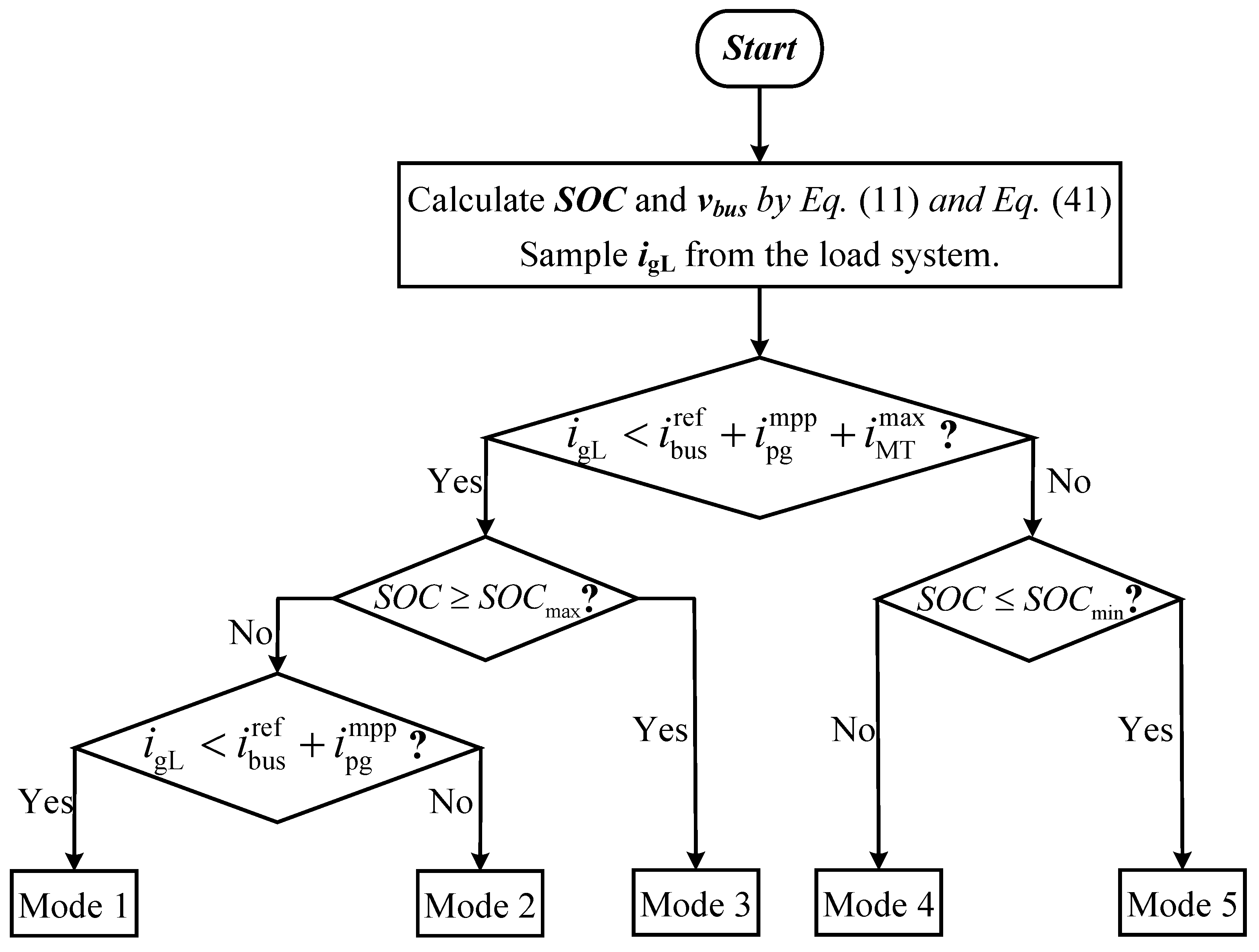
4.1.2. Bus Control Layer

Due to the relatively independent control systems of device-level units, coordinated control cannot be achieved, necessitating higher-level control for scheduling decisions. This paper selects the bus control layer as the second layer of control for the island DMG, monitoring the DC bus voltage and current in real time, as well as the output currents of each device-level unit. Based on the actual operational state, it switches to the appropriate operational mode, adjusts the control methods and reference values of each device-level unit, and stabilizes the DC bus voltage [35].

The operational strategy of the bus control layer is to consider the SOC of the energy storage unit based on the size of the load current demand ($i_{\mathrm{gL}}$), dividing into five operational modes as shown in Figure 11, where $i_{\mathrm{bus}}^{\mathrm{ref}}$, $i_{\mathrm{pg}}^{\mathrm{mpp}}$, and $i_{\mathrm{MT}}^{max}$ represent the reference output current of the DC bus, the output current of the PV generation unit in MPPT mode, and the maximum output current of the MT generation unit, respectively.

Defining the reference value of the DC bus voltage as $v_{\mathrm{bus}\_\mathrm{ref}}$, the deviation of the bus voltage can be represented by $err=v_{\mathrm{bus}\_\mathrm{ref}}-v_{\mathrm{bus}}$. The specific control process for each mode is as follows:

• Mode 1: The PV generation unit operates in MPPT mode, and the BAT storage unit charges rapidly at maximum charging current. The bus control layer adjusts the output of the MT generation unit according to Equation (32) to stabilize the bus voltage, where $\alpha$ is a proportional coefficient.

  $$v_{\mathrm{dc}}^{\ast }[k+1]=v_{\mathrm{dc}}^{\ast }\left[k\right]+\alpha ·err$$

  (32)
• Mode 2: The PV generation unit operates in MPPT mode, and the MT generation unit reaches its rated power. The bus control layer adjusts the charging power of the BAT storage unit according to Equation (33) to stabilize the bus voltage, where $\beta$ is a proportional coefficient.

  $$i_{\mathrm{L}2\_\mathrm{ref}}[k+1]=i_{\mathrm{L}2\_\mathrm{ref}}\left[k\right]+\beta ·err$$

  (33)
• Mode 3: If the BAT storage unit is fully charged and disabled in Mode 1, the PV generation unit operates in CV mode; if the BAT storage unit is fully charged and disabled in Mode 2, the PV generation unit operates in MPPT mode. The bus control layer adjusts the output of the MT generation unit according to Equation (32) to stabilize the bus voltage.
• Mode 4: The PV generation unit operates in MPPT mode, and the MT generation unit reaches its rated power. The bus control layer adjusts the discharge power of the BAT storage unit according to Equation (34) to stabilize the bus voltage, where $\gamma$ is a proportional coefficient.

  $$V_{\mathrm{H}\_\mathrm{ref}}[k+1]=v_{\mathrm{H}\_\mathrm{ref}}\left[k\right]+\gamma ·err$$

  (34)
• Mode 5: The PV generation unit operates in MPPT mode, and the MT generation unit reaches its rated power. If the BAT storage unit is disabled due to insufficient capacity, the bus control layer needs to dump non-critical loads to maintain bus voltage stability.

The criterion for stability of the DC bus voltage is whether the bus voltage error $err$ is less than a given convergence threshold ${\epsilon }_{\mathrm{bus}}$.

4.2. Multi-Energy Dispatch Strategy

The operation mode of RIES varies depending on the different operational modes of each unit. In this paper, the MT generates both electricity and heat by burning natural gas with its heat-to-electricity ratio being a constant; the EB is an electro-thermal coupling device that converts electricity into heat with its thermal inertia being neglected in steady-state flow calculation due to the large difference in time scale between DMG and DHN. These two devices enable RIESs to operate in two modes: thermal-led and electricity-led.

4.2.1. Thermal-Led

The amount of natural gas consumed by the MT is determined by the thermal load ${\Phi }_{\mathrm{heat}}$ of the DHN. If the thermal load demand exceeds the heating capacity of the MT device, the EB supplements the thermal load difference $\Delta {\Phi }_{\mathrm{heat}}$.

When ${\Phi }_{\mathrm{heat}}\le {\Phi }_{\mathrm{MT}}^{max}$:

$$\begin{array}{cc}\hfill {\Phi }_{\mathrm{g},\mathrm{MT}}& ={\Phi }_{\mathrm{heat}}/{\eta }_{\mathrm{MT}}^{\mathrm{gh}}\hfill \\ \hfill \Delta {\Phi }_{\mathrm{heat}}& =0\hfill \end{array}$$

(35)

When ${\Phi }_{\mathrm{heat}}>{\Phi }_{\mathrm{MT}}^{max}$:

$$\begin{array}{cc}\hfill {\Phi }_{\mathrm{g},\mathrm{MT}}& ={\Phi }_{\mathrm{MT}}^{max}/{\eta }_{\mathrm{MT}}^{\mathrm{gh}}\hfill \\ \hfill \Delta {\Phi }_{\mathrm{heat}}& ={\Phi }_{\mathrm{heat}}-{\Phi }_{\mathrm{MT}}^{max}\hfill \end{array}$$

(36)

The electrical power consumed by the EB device is:

$$\begin{array}{c}\hfill P_{\mathrm{EB}}=\Delta {\Phi }_{\mathrm{heat}}/{\eta }_{\mathrm{EB}}\end{array}$$

(37)

where ${\Phi }_{\mathrm{g},\mathrm{MT}}$ and ${\Phi }_{\mathrm{MT}}^{max}$ are the energy obtained from the NGN and the maximum thermal power output and heat production efficiency of MT; ${\eta }_{\mathrm{MT}}^{\mathrm{gh}}$ and ${\eta }_{\mathrm{EB}}$ are the heat production efficiencies of MT and EB, respectively.

4.2.2. Electricity-Led

The amount of natural gas consumed by the MT is determined by the electrical load $P_{\mathrm{CPL}}$, with the generated thermal energy supplied to the DHN together with the EB.

When $P_{\mathrm{CPL}}\le P_{\mathrm{MT}}^{max}$:

$$\begin{array}{cc}\hfill {\Phi }_{\mathrm{g},\mathrm{MT}}& =P_{\mathrm{CPL}}/{\eta }_{\mathrm{MT}}^{\mathrm{ge}}\hfill \\ \hfill \Delta P_{\mathrm{CPL}}& =0\hfill \end{array}$$

(38)

When $P_{\mathrm{CPL}}>P_{\mathrm{MT}}^{max}$:

$$\begin{array}{cc}\hfill {\Phi }_{\mathrm{g},\mathrm{MT}}& =P_{\mathrm{MT}}^{max}/{\eta }_{\mathrm{MT}}^{\mathrm{ge}}\hfill \\ \hfill \Delta P_{\mathrm{CPL}}& =P_{\mathrm{CPL}}-P_{\mathrm{MT}}^{max}\hfill \end{array}$$

(39)

The electrical power consumed by the EB device is:

$$\begin{array}{c}\hfill P_{\mathrm{EB}}=({\Phi }_{\mathrm{heat}}-{\Phi }_{\mathrm{g},\mathrm{MT}}·{\eta }_{\mathrm{MT}}^{\mathrm{gh}})/{\eta }_{\mathrm{EB}}\end{array}$$

(40)

where $P_{\mathrm{MT}}^{max}$ and ${\eta }_{\mathrm{MT}}^{\mathrm{ge}}$ are, respectively, the maximum electrical power output and electrical efficiency of MT; $\Delta P_{\mathrm{CPL}}$ is the electrical power compensated.

For DHNs and NGNs with long time scales and constant operational states, the decomposed energy flow method offers better speed and accuracy [12]. It typically starts by calculating the independent loads at the coupling nodes of each energy network, with each network then iterating based on its constraints. The multi-energy dispatch process for RIESs is shown in Figure 12, with the solving steps as follows:

• To conduct hydraulic flow calculation, after correcting the flow error, perform thermal flow calculation and calculate the total thermal power ${\Phi }_{heat}$ at the DHN source, i.e., the thermal load demand, based on Equation (18).
• Based on the thermal load demand and dispatch mode, calculate the electrical power output of MT, the electrical power consumed by EB, and the fuel consumption of MT. The HIS is used to control the DMG until the DC bus voltage converges.
• Convert the fuel quantity $f_{\mathrm{MT}}$ to natural gas mass flow rate using Equation (41), and input it into MT coupling node for gaseous flow calculation until flow error is corrected.

  $$\begin{array}{c}\hfill f_{\mathrm{MT}}=\frac{{\Phi }_{\mathrm{g},\mathrm{MT}}}{LHV}\frac{1}{3600}\end{array}$$

  (41)
  Here, $LHV$ is the lower heating value of natural gas, taken as 13.52 kWh/kg.
• Determine if the DHN, NGN, and DMG all meet convergence criteria. If they do, the process ends; otherwise, continue with flow calculation.

5. Real-Time Platform Implementation and Experimental Verification

To validate the accuracy of the device-level unit models and the efficiency and flexibility of the energy control strategies, this paper presents a design for a real-time simulation platform based on DSPs, as shown in Figure 13. The communication protocol between the DSPs requires network communication rate of 1000 Mbps to support high-speed data transfer, ensuring real-time performance. Communication latency is maintained below 10 microseconds to prevent any adverse impact on system performance. The DSPs are divided into a simulation group and a control group, where the simulation group is used to run the device-level unit and energy network models; the control group receives computational results from the simulation group in sequence via the TCP/IP protocol and controls them according to HIS and MEDS. The PC can monitor and modify the parameters of the control group through the Modbus TCP protocol to achieve scheduling simulations under different conditions. Subsequently, an 18-node RIES case is proposed to conduct dispatch experiments in thermal-led and electricity-led modes. The hierarchical island strategy and multi-energy dispatch strategy implemented in this study have a computational complexity of $O\left(n^2\right)$, where n represents the number of nodes in the energy system. This quadratic complexity arises from the need to manage multiple interactions between different energy sources and loads in real time.

5.1. Iteration Technique

To transform the averaged switch models of device-level units within the DMG, derived in Section 2, into iterative equation sets executable by DSP, this paper selects appropriate transformation methods based on the model order: for open-loop control models with lower orders, such as electrical power transmission lines, first-order forward Euler discretization is used; for transfer functions with closed-loop control and higher orders, bilinear transformation is employed for discretization.

The device-level units often contain numerous state variables that are closely interconnected. Using the conventional forward Euler method can be slow, resulting in lengthy convergence times. To address this, an iterative acceleration algorithm is proposed on the basis of the discretized equations. This method enhances the first-order forward Euler approach by utilizing the updated values of a state variable once its iteration is complete for calculating the next related state variable. For instance, in an N-order system, this approach leads to a set of differential equations involving N state variables:

$$\left\{\begin{array}{c}{\dot{z}}_1=f_1\left(z_1,\cdots ,z_n\right)\\ {\dot{z}}_2=f_2\left(z_1,\cdots ,z_n\right)\\ \cdots \cdots \\ {\dot{z}}_n=f_n\left(z_1,\cdots ,z_n\right)\end{array}\right.$$

(42)

By applying the acceleration algorithm, we can obtain the following iterative equations:

$$\begin{array}{c}{z}_1[k+1]=f_1\left(z_1\left[k\right],z_2\left[k\right],\cdots ,z_n\left[k\right]\right)\hfill \\ z_2[k+1]=f_2\left(z_1[k+1],z_2\left[k\right],\cdots ,z_n\left[k\right]\right)\hfill \\ \cdots \cdots \hfill \\ z_n[k+1]=f_n\left(z_1[k+1],z_2[k+1],\cdots ,z_{n-1}[k+1],z_n\left[k\right]\right)\hfill \end{array}$$

(43)

5.2. Case Configuration

The RIES case study, as shown in Figure 14, comprises a five-node DMG, a six-node DHN, and a seven-node NGN. The DMG is composed of RIES device-level units, including PV generation, MT generation, BAT storage, and load. The load unit consist of resistive loads EB and CPL (such as electrical vehicle charger). The stable DC bus voltage is 750 V. The maximum power of PV at S = 1000 $\mathrm{W}/{\mathrm{m}}^2$ and T = 298 K is 25 kW; the rated power of the MT generation unit is 42 kW, with a rated speed for the PMSG of 12,000 r/m; the initial SOC of BAT storage unit is 0.65. In the energy conversion equipment, the heat production efficiency of MT (${\eta }_{\mathrm{MT}}^{\mathrm{gh}}$) is 0.4, and its electrical efficiency (${\eta }_{\mathrm{MT}}^{\mathrm{ge}}$) is 0.3; the efficiency of the EB (${\eta }_{\mathrm{EB}}$) is 0.85. The specific circuit parameters of each device-level unit are presented in

Table A1. Circuit parameters of 5-node DMG.

System	Parameters	Value
DC Grid Backbone	$E_{bus}$, $r_{bus}$	760 V, 0.5 $\Omega$
	$C_{bus}$	2.2 mF
PV Generation Unit	$C_p$, $C_1$	470 $\mathsf{\mu }$F, 1 mF
	$L_1$, $L_{g1}$	2.5 mH, 0.1 mH
	$r_{g1}$	1 $\Omega$
	$k{p}_{mpp}$, $k{i}_{mpp}$	0.25, 0.105
	$k{p}_{cv}$, $k{i}_{cv}$	0.00025, 2.5
MT Generation Unit	$R_s$, $C_{dc}$	5 $\Omega$, 2.2mF
	${\Phi }_f$, D	0.2475 $\mathrm{V}·\mathrm{s}$, 0.0005
	J, $p_n$	0.001 $\mathrm{kg}·{\mathrm{m}}^2$, 1
	$L_s$, $L_{g2}$	5.95 mH, 0.1 mH
	$r_{g2}$	0.5 $\Omega$
	$k{p}_{isq}$, $k{i}_{isq}$	298.3, 0.0012
	$k{p}_{vdc}$, $k{i}_{vdc}$	3 $\times {10}^3$, 1.75 $\times {10}^{-5}$
BAT Storage Unit	$E_{bat}$, $C_d$	400 V, 1 mF
	$r_b$, $r_{g1}$	0.5 $\Omega$, 0.5 $\Omega$
	$C_{2H}$, $C_{2L}$	1 mF, 1 mF
	$SO{C}_{\min }$, $SO{C}_{\max }$	0.4, 0.9
	$k{p}_{buck}$, $k{i}_{buck}$	0.001, 1.1948
	$k{p}_{boost}$, $k{i}_{boost}$	0.00025, 0.5
Load Unit	$C_3$, $C_4$	470 $\mathsf{\mu }$F, 1 mF
	$L_3$	1.5 mH
	$k{p}_{CPL}$, $k{i}_{CPL}$	0, −0.13529

.

The DHN includes a symmetrical six-node supply water network and a six-node return water network. A heat source is located at nodes 1–7, operating under fixed outlet pressure and temperature modes to regulate the overall temperature of the DHN; simulated users are placed between nodes 6–12, 4–10, and 5–11, where the mass flow rate in their branches is determined by pressure, and the heat exchange power is given; a regulating valve operating in a fixed opening mode is installed between branch 2–6; and a booster pump operating in a fixed speed mode is installed between branches 3–4 and 3–5. Specific pipeline branch parameters are presented in

Table A2. Pipeline parameters of 6-node DHN.

Pipe	Length	Diameter	Fraction	Heat Dissipation	${\mathit{T}}_{\mathbf{loss}}$
1–2	30 m	0.04 m	0.05	0.5	0
2–3	50 m	0.04 m	0.05	0.5	0
3–5	30 m	0.025 m	0.05	0.5	0
2–6	40 m	0.025 m	0.05	0.5	0
3–4	40 m	0.025 m	0.05	0.5	0
8–7	10 m	0.04 m	0.05	0.5	0
9–8	50 m	0.04 m	0.05	0.5	0
11–9	30 m	0.025 m	0.05	0.5	0
12–8	40 m	0.025 m	0.05	0.5	0
10–9	40 m	0.025 m	0.05	0.5	0
6–12	2 m	0.02 m	0.08	0	20 ℃
4–10	2 m	0.02 m	0.08	0	25 ℃
5–11	2 m	0.02 m	0.08	0	20 ℃

, with the control valve and booster pump parameters shown in

Table A3. Device parameters in 6-node DHN.

Device	Parameters
Valve	$k_v=0.613$
Pump	$k_{p1}=-0.0475;k_{p2}=-0.0277;k_{p3}=0.7281;\omega =0.75$

.

In this DHN, node 1 is set as a fixed pressure node with a given supply water pressure of 3000 Pa. Node 1 is also the thermal source, with a given temperature; the remaining nodes are defined as fixed injection nodes, where node 7 has a given mass flow rate of 0.15 kg/s, and the mass flow rates for the other nodes are zero. The initial base value for mass flow rate in each branch is set to 0.05 kg/s, with a convergence threshold of 1 $\times {10}^{-5}$ and an update step size of 0.7.

The seven-node natural gas network includes six pipeline branches; gas sources are located at nodes 4 and 7, supplying natural gas to the network; natural gas loads are placed at nodes 1, 3, and 5, with node 5 being the MT coupling node; a compressor is set between branch 6–2 to increase the gas pressure by 2 kPa. Specific parameters for the pipeline branches are shown in

Table A4. Pipeline parameters of 7-node NGN.

Pipe	Length	Diameter	Fraction
2–1	20 m	0.06 m	0.25
3–2	10 m	0.06 m	0.25
4–3	50 m	0.08 m	0.25
6–2	10 m	0.06 m	0.25
6–5	20 m	0.06 m	0.25
7–6	30 m	0.08 m	0.25

.

In the NGN, nodes 4 and 7 are set as fixed pressure nodes, with node 4 having a gas pressure of 10 kPa and node 7 a pressure of 8 kPa. The remaining nodes are defined as fixed injection nodes, with nodes 1 and 3 given mass flow rates of 0.0025 kg/s, nodes 2 and 6 given zero mass flow rate, and node 5 providing the gas fuel for the MT. The base gas flow velocity for each branch is set to 10 m/s, with a convergence threshold of 1 $\times {10}^{-3}$ and a base value update step size of 0.75.

5.3. Experimental Results

The real-time platform selects the TMS320F28335 DSP as its core processing unit, with the onboard W5300 network chip enabling data communication within the hardware platform; it is paired with the DAC8552 for observing the DA conversion results of the model computations through an oscilloscope. The physical platform is shown in Figure 15, where the DSP module group consists of four DSPs, one of which is for the control group DSP; the remaining simulation group DSPs run models of the DMG, DHN, and NGN, respectively.

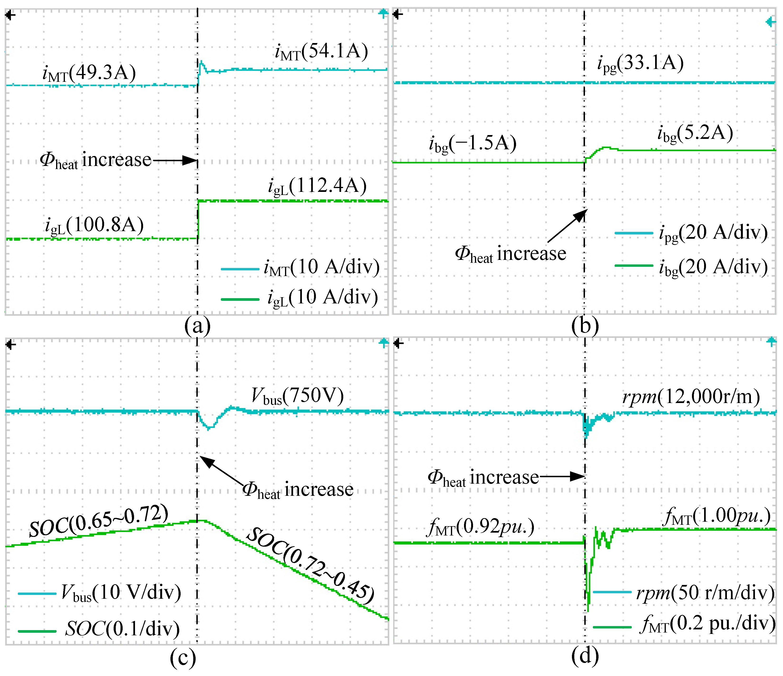
5.3.1. Thermal-Led Experiment

In the thermal-led mode, the output power of MT is determined by the thermal load, with the electrical load remaining constant. Adjusting the temperature of the heat source facilitates changes in the thermal load. In this experiment, the electrical load, specifically the CPL load $P_{\mathrm{elec}}$, is kept constant at 75 kW, and the temperature of the heat source is raised from 80 °C to 100 °C. Figure 16a depicts the iteration of mass flow rates for the 5 branches of the supply water network and the error correction process, which converges after nine iterations. The changes in water pressure and temperature are shown in Figure 16b.

As shown in Figure 17a–c, before the increase in thermal load, it is less than the maximum heat production capacity of MT, and heating is provided solely by MT with EB not operational. At this point, the load current $i_{gL}$ in DMG corresponds only to the electrical load demand, and the SOC of the storage is below its maximum value. According to HIS, it is indicated that the DMG is in mode 2, with the PV generation unit operating in MPPT mode; HIS adjusts the charging power of the BAT to stabilize the DC bus voltage at 750 V, with SOC in an increasing state.

When the thermal load exceeds the heat production limit of MT, MT operates at its rated power, and its output current rises from 49.3 A to the rated current of 54.1 A; EB increases its power consumption to compensate for the thermal load difference, causing the load current to increase from 100.8 A to 112.4 A. At this point, HIS indicates that the DMG switches from mode 2 to mode 4. The PV generation unit continues to operate in MPPT control mode; the BAT storage unit switches from charging to discharging, with its output current changing from −1.5 A to 5.2 A, and SOC begins to decrease; the DC bus voltage experiences a temporary drop at the moment of thermal load increase, and HIS quickly switches the BAT operation state and adjusts the discharge power to stabilize the DC bus voltage at 750 V.

The increase in MT output power causes the electromagnetic torque $T_e$ of the PMSG to increase, and since the mechanical torque $T_m<T_e$, the speed temporarily drops. Subsequently, the fuel demand for MT increases from 0.92 pu. to 1.0 pu., the output mechanical torque $T_m$ increases, and the speed recovers to 12,000 r/m, as shown in Figure 17d.

Using the stabilized fuel input value of the MT, the steady-state flow calculation for the NGN converges after eight and seven iterations, as shown in Figure 18. The gas pressure at each node and the mass flow rate through each branch are listed in

Table 1. Flow calculation results of the NGN in thermal-led mode.

Node Gas Pressure (Pa)			Branch Mass Flow Rates (kg/s)
Node	Before	After	Branch	Before	After
1	9640.55	9629.93	2–1	0.0025	0.0025
2	9795.54	9785.08	3–2	0.00113	0.0012
3	9810.94	9802.70	4–3	0.00363	0.0037
4	10,000	10,000	6–2	0.00137	0.0013
5	7607.72	7553.61	6–5	0.00265	0.00287
6	7824.96	7811.33	6–7	0.00402	0.00417
7	8000	8000

. Except for the gas source nodes, the gas pressure at other nodes decreases with the increase in thermal load. Due to the presence of the compressor, the mass flow rate in branch 6-2 decreases, while the mass flow rates in the other branches increase due to the increase in thermal load.

5.3.2. Electricity-Led Experiment

In the electricity-led mode, the electrical load determines the output of the MT, with the thermal load remaining constant, and changes to the electrical load are achieved by adjusting the CPL power. In this experiment, the temperature of the heating network’s heat source is kept constant at 100 °C, and the electrical load is increased from 32 kW to 80 kW.

The iteration of mass flow rates for the five branches of the supply water network and the error correction process in this mode are the same as the thermal-led experiment, as shown in Figure 16a. The hydraulic flow calculation shows the water pressure at various nodes as depicted in Figure 16b, with the node temperature indicated by the red curve.

As shown in Figure 19a–c, before the increase in electrical load, it is below the maximum electrical power output of MT. At this time, the thermal load within the system exceeds the heat production capacity of MT, compensated by EB for the thermal load difference. The load current $i_{\mathrm{gL}}$ is 77.8 A, and the SOC of the BAT is below its maximum value, indicating that the DMG is in mode 2, with the PV generation unit operating in MPPT mode; HIS adjusts the BAT charging power to stabilize the DC bus voltage at 750 V, with SOC in a rising state.

After the increase in electrical load, exceeding the maximum electrical power output of MT, MT operates at its rated power, with its output current rising from 39.4 A to the rated current of 54.4 A. At this time, the load current rises from 77.8 A to 118.1 A, indicating that the DMG switches from mode 2 to mode 4, with the PV generation unit still operating in MPPT mode, outputting 33.1 A; the BAT storage unit switches from charging to discharging, with its output current changing from −15.3 A to 10.5 A, and SOC begins to decrease. The DC bus voltage undergoes a transient drop at electrical load increase instant, with HIS quickly switching the BAT operation state and adjusting the discharge power to stabilize the DC bus voltage at 750 V. Changes in fuel demand and speed of MT are shown in Figure 19d.

Using the stable value of fuel demand calculated with Equation (41), the mass flow rate $G_{\mathrm{b},\mathrm{MT}}$ at the MT coupling node is determined for steady-state flow calculations. The iterative process of the gaseous velocity base values is shown in Figure 20, which converged after eight iterations. The gas pressure at each node and the mass flow rate through each branch are listed in

Table 2. Flow calculation results of the NGN in electricity-led mode.

Node Gas Pressure (Pa)			Branch Mass Flow Rates (kg/s)
Node	Before	After	Branch	Before	After
1	9657.92	9628.56	2–1	0.0025	0.0025
2	9812.64	9783.73	3–2	0.00099	0.00121
3	9824.60	9801.64	4–3	0.00349	0.00371
4	10,000	10,000	6–2	0.00151	0.00129
5	7692.76	7546.53	6–5	0.00225	0.0029
6	7847.85	7809.59	7–6	0.00375	0.00419
7	8000	8000

. These results highlight how the network responds to changes in demand, with pressure adjustments across nodes and variations in mass flow rates through the branches to accommodate the energy needs in the electricity-led mode.

6. Conclusions

This paper introduced a real-time simulation platform for a RIES that includes DMG, DHN, and NGN. To facilitate real-time multi-energy flow simulation of the RIES, it first developed averaged switch models and control methods for device-level units within the DMG, along with the circuit-dual models for the DHN and NGN. The hierarchical island strategy (HIS) and the multi-energy dispatch strategy (MEDS) were proposed for multi-energy flow control and calculation. Validation was performed through designed case studies and the constructed experimental platform. Experimental results demonstrated that the HIS can quickly adjust the operation modes of device-level units in real time to ensure bus voltage stability. Simultaneously, the MEDS incorporating energy conversion devices such as MT and EB, employed the decomposed flow method for simulating multi-energy flows of RIES under different operational modes. In conclusion, the developed real-time simulation platform not only maintained the stable operation of the DMG, but also effectively managed energy dispatch for the DHN and NGN. This work contributed theoretical and practical insights for the control and simulation of RIES, thus providing practical references for the simulation, design, and operation of integrated energy systems.

In the future, our research could explore advanced optimization algorithms to enhance the efficiency of MEDS, potentially integrating AI and machine learning to predict and manage energy demands dynamically. Additionally, investigating the long-term resilience of RIES against various environmental and operational stresses could further solidify the practical applicability of the simulation platform. Developing expandable models that can be adapted to larger or more complex energy networks may also be a fruitful direction, aiming to support the growing needs of urban energy systems worldwide.

References

1. Stennikov, V.; Barakhtenko, E.; Sokolov, D.; Zhou, B. Current State of Research on the Energy Management and Expansion Planning of Integrated Energy Systems. Energy Rep. 2022, 8, 10025–10036. [Google Scholar] [CrossRef]
2. Zhang, H.; Wang, W.; Zhu, L.; Sun, Z.; Ma, D.; Chen, W. Prospect of Typical Application of Integrated Energy System. IOP Conf. Ser. Earth Environ. Sci. 2021, 651, 022030. [Google Scholar] [CrossRef]
3. Chicco, G.; Riaz, S.; Mazza, A.; Mancarella, P. Flexibility From Distributed Multienergy Systems. Proc. IEEE 2020, 108, 1496–1517. [Google Scholar] [CrossRef]
4. Cheng, H.; Hu, X.; Wang, L.; Liu, Y.; Yu, Q. Review on research of regional integrated energy system planning. Autom. Electr. Power Syst. 2019, 43, 2–13. [Google Scholar]
5. Fan, H.; Wang, C.; Liu, L.; Li, X. Review of Uncertainty Modeling for Optimal Operation of Integrated Energy System. Front. Energy Res. 2022, 9, 641337. [Google Scholar] [CrossRef]
6. Ilyushin, P.; Gerasimov, D.; Suslov, K. Method for Simulation Modeling of Integrated Multi-Energy Systems Based on the Concept of an Energy Hub. Appl. Sci. 2023, 13, 7656. [Google Scholar] [CrossRef]
7. Qiao, Y.; Hu, F.; Xiong, W.; Li, Y. Energy hub-based configuration optimization method of integrated energy system. Int. J. Energy Res. 2022, 46, 23287–23309. [Google Scholar] [CrossRef]
8. Chen, B.; Guo, Q.; Yin, G.; Wang, B.; Pan, Z.; Chen, Y.; Wu, W.; Sun, H. Energy-Circuit-Based Integrated Energy Management System: Theory, Implementation, and Application. Proc. IEEE 2022, 110, 1897–1926. [Google Scholar] [CrossRef]
9. Yang, J.; Zhang, N.; Botterud, A.; Kang, C. On An Equivalent Representation of the Dynamics in District Heating Networks for Combined Electricity-Heat Operation. IEEE Trans. Power Syst. 2020, 35, 560–570. [Google Scholar] [CrossRef]
10. Li, M.; Ye, J. Fractional Order Modeling of Thermal Circuits for an Integrated Energy System Based on Natural Transformation. Electronics 2022, 11, 914. [Google Scholar] [CrossRef]
11. Qu, L.; Ouyang, B.; Yuan, Z.; Zeng, R. Steady-State Power Flow Analysis of Cold-Thermal-Electric Integrated Energy System Based on Unified Power Flow Model. Energies 2019, 12, 4455. [Google Scholar] [CrossRef]
12. Massrur, H.R.; Niknam, T.; Aghaei, J.; Shafie-khah, M.; Catalao, J.P.S. Fast Decomposed Energy Flow in Large-Scale Integrated Electricity-Gas-Heat Energy Systems. IEEE Trans. Sustain. Energy 2018, 9, 1565–1577. [Google Scholar] [CrossRef]
13. Zhu, M.; Xu, C.; Dong, S.; Tang, K.; Gu, C. An Integrated Multi-Energy Flow Calculation Method for Electricity-Gas-Thermal Integrated Energy Systems. Prot. Control Mod. Power Syst. 2021, 6, 5. [Google Scholar] [CrossRef]
14. Liang, Z.; Mu, L. Unified calculation of multi-energy flow for integrated energy system based on difference grid. J. Renew. Sustain. Energy 2022, 14, 066301. [Google Scholar] [CrossRef]
15. Xue, Y.; Li, Z.; Lin, C.; Guo, Q.; Sun, H. Coordinated Dispatch of Integrated Electric and District Heating Systems Using Heterogeneous Decomposition. IEEE Trans. Sustain. Energy 2020, 11, 1495–1507. [Google Scholar] [CrossRef]
16. Yao, S.; Gu, W.; Wu, J.; Lu, H.; Zhang, S.; Zhou, Y.; Lu, S. Dynamic energy flow analysis of the heat-electricity integrated energy systems with a novel decomposition-iteration algorithm. Appl. Energy 2022, 322, 119492. [Google Scholar] [CrossRef]
17. Yao, S.; Gu, W.; Wu, J.; Qadrdan, M.; Lu, H.; Lu, S.; Zhou, Y. Fast and generic energy flow analysis of the integrated electric power and heating networks. IEEE Trans. Smart Grid 2023, 15, 355–367. [Google Scholar] [CrossRef]
18. Sergi, B.; Pambour, K. An evaluation of co-simulation for modeling coupled natural gas and electricity networks. Energies 2022, 15, 5277. [Google Scholar] [CrossRef]
19. Gusain, D.; Cvetković, M.; Palensky, P. Simplifying multi-energy system co-simulations using energysim. SoftwareX 2022, 18, 101021. [Google Scholar] [CrossRef]
20. El Zerk, A.; Ouassaid, M. Real-time fuzzy logic based energy management system for microgrid using hardware in the loop. Energies 2023, 16, 2244. [Google Scholar] [CrossRef]
21. Guan, A.; Zhou, S.; Gu, W.; Lu, S.; Wu, Z.; Gao, M. An Experimental Platform of Heating Network Similarity Model for Test of Integrated Energy Systems. IEEE Trans. Ind. Inform. 2023, 20, 5517–5528. [Google Scholar] [CrossRef]
22. Meng, Q.; Jin, X.; Luo, F.; Wang, Z.; Hussain, S. Distributionally Robust Scheduling for Benefit Allocation in Regional Integrated Energy System with Multiple Stakeholders. J. Mod. Power Syst. Clean Energy 2024, 321, 119202. [Google Scholar]
23. Tan, J.; Wu, Q.; Zhang, X. Optimal Planning of Integrated Electricity and Heat System Considering Seasonal and Short-Term Thermal Energy Storage. IEEE Trans. Smart Grid 2023, 14, 2697–2708. [Google Scholar] [CrossRef]
24. Ma, Y.; Han, X.; Zhang, T.; Li, A.; Song, Z.; Li, T.; Wang, Y. Research on station-network planning of electricity-thermal-cooling regional integrated energy system considering multiple-load clusters and network costs. Energy 2024, 297, 131281. [Google Scholar] [CrossRef]
25. Al-Ismail, F.S. DC Microgrid Planning, Operation, and Control: A Comprehensive Review. IEEE Access 2021, 9, 36154–36172. [Google Scholar] [CrossRef]
26. Kyriakou, D.G.; Kanellos, F.D. Energy and power management system for microgrids of large-scale building prosumers. IET Energy Syst. Integr. 2023, 5, 228–244. [Google Scholar] [CrossRef]
27. Huang, C.; Wang, J.; Deng, S.; Yue, D. Real-time distributed economic dispatch scheme of grid-connected microgrid considering cyberattacks. IET Renew. Power Gener. 2020, 14, 2750–2758. [Google Scholar] [CrossRef]
28. Pradhan, C.; Senapati, M.K.; Ntiakoh, N.K.; Calay, R.K. Roach Infestation Optimization MPPT Algorithm for Solar Photovoltaic System. Electronics 2022, 11, 927. [Google Scholar] [CrossRef]
29. Rowen, W.I. Simplified Mathematical Representations of Heavy-Duty Gas Turbines. J. Eng. Power 1983, 105, 865–869. [Google Scholar] [CrossRef]
30. Hackl, C.M.; Pecha, U.; Schechner, K. Modeling and Control of Permanent-Magnet Synchronous Generators Under Open-Switch Converter Faults. IEEE Trans. Power Electron. 2019, 34, 2966–2979. [Google Scholar] [CrossRef]
31. Chen, B.; Wu, W.; Guo, Q.; Sun, H. An efficient optimal energy flow model for integrated energy systems based on energy circuit modeling in the frequency domain. Appl. Energy 2022, 326, 119923. [Google Scholar] [CrossRef]
32. Khan, R.; Nasir, M.; Schulz, N.N. An Optimal Neighborhood Energy Sharing Scheme Applied to Islanded DC Microgrids for Cooperative Rural Electrification. IEEE Access 2023, 11, 116956–116966. [Google Scholar] [CrossRef]
33. Shafiee, Q.; Dragičević, T.; Vasquez, J.C.; Guerrero, J.M. Hierarchical Control for Multiple DC-Microgrids Clusters. IEEE Trans. Energy Convers. 2014, 29, 922–933. [Google Scholar] [CrossRef]
34. Barati, F.; Ahmadi, B.; Keysan, O. A Hierarchical Control of Supercapacitor and Microsources in Islanded DC Microgrids. IEEE Access 2023, 11, 7056–7066. [Google Scholar] [CrossRef]
35. Krishan, R.; Rohith, Y. Load and Generation Converters Control Strategy to Enhance the Constant Power Load Stability Margin in a DC Microgrid. IEEE Access 2024, 12, 35972–35983. [Google Scholar] [CrossRef]
Figure 1. Boost converter circuit topology.
Energies 17 03211 g001
Figure 2. PMSG-VSR circuit topology.
Energies 17 03211 g002
Figure 3. TL buck–boost converter circuit topology.
Energies 17 03211 g003
Figure 4. Buck converter circuit topology.
Energies 17 03211 g004
Figure 5. Equivalent circuit model of the hydraulic branch [31].
Energies 17 03211 g005
Figure 6. Equivalent circuit model of the valve and booster pump.
Energies 17 03211 g006
Figure 7. Equivalent circuit model of the thermal branch [31].
Energies 17 03211 g007
Figure 8. Equivalent circuit model of the gaseous branch [8].
Energies 17 03211 g008
Figure 9. Control block diagram of device-level units. (a): maximum power point tracking (MPPT) control and constant voltage (CV) control of PV generation unit; (b): control of MT generation unit; (c): constant current (CC) and CV control of BAT storage unit; (d): control of load unit.
Energies 17 03211 g009
Figure 10. Equivalent circuit structure of the island DMG.
Energies 17 03211 g010
Figure 11. Operating mode decision making flow chart.
Energies 17 03211 g011
Figure 12. Flowchart of multi-energy dispatch for RIES.
Energies 17 03211 g012
Figure 13. Design of DSP-based real-time simulation platform.
Energies 17 03211 g013
Figure 14. RIES case study consisting of a 5-node DMG, a 6-node DHN, and a 7-node NGN.
Energies 17 03211 g014
Figure 15. Real-time simulation platform diagram.
Energies 17 03211 g015
Figure 16. Flow calculation results of DHN in thermal-led mode.
Energies 17 03211 g016
Figure 17. Experimental results of DMG in thermal-led mode (x-axis: 500 ms/div). (a): currents of MT generation unit and load unit; (b): currents of PV generation unit and energy storage unit; (c): DC bus voltage and SOC; (d): rotation speed and fuel demand of MT.
Energies 17 03211 g017
Figure 18. Iteration process of gaseous velocity base values in thermal-led mode.
Energies 17 03211 g018
Figure 19. Experimental results of DMG in electricity-led mode (x-axis: 500 ms/div). (a): currents of MT generation unit and load unit; (b): currents of PV generation unit and energy storage unit; (c): DC bus voltage and SOC; (d): rotation speed and fuel demand of MT.
Energies 17 03211 g019
Figure 20. Iteration process of gaseous velocity base values in electricity-led mode.
Energies 17 03211 g020