Abstract
Financial markets are increasingly interlinked. Therefore, this study explores the complex relationships between the Tadawul All Share Index (TASI), West Texas Intermediate (WTI) crude oil prices, and Bitcoin (BTC) returns, which are pivotal to informed investment and risk-management decisions. Using copula-based models, this study identified Student’s t copula as the most appropriate one for encapsulating the dependencies between TASI and BTC and between TASI and WTI prices, highlighting significant tail dependencies. For the BTC–WTI relationship, the Frank copula was found to have the best fit, indicating nonlinear correlation without tail dependence. The predictive power of the identified copulas were compared to that of Long Short-Term Memory (LSTM) networks. The LSTM models demonstrated markedly lower Root Mean Squared Error (RMSE), Mean Absolute Error (MAE), and Mean Absolute Scaled Error (MASE) across all assets, indicating higher predictive accuracy. The empirical findings of this research provide valuable insights for financial market participants and contribute to the literature on asset relationship modeling. By revealing the most effective copulas for different asset pairs and establishing the robust forecasting capabilities of LSTM networks, this paper sets the stage for future investigations of the predictive modeling of financial time-series data. The study highlights the potential of integrating machine-learning techniques with traditional econometric models to improve investment strategies and risk-management practices.
1. Introduction
The intersection of traditional stock market indices, digital currencies, and commodity prices presents a unique opportunity to explore the dynamic and complex relationships within the global financial ecosystem. The Tadawul All Share Index (TASI) represents the Saudi Arabian stock market and encapsulates the economic pulse of one of the world’s largest oil-exporting nations. Bitcoin, a decentralized digital currency introduced by [1], has emerged as a novel asset class, challenging conventional financial paradigms through its rapid growth and volatility. Similarly, West Texas Intermediate (WTI) crude oil prices play a pivotal role in energy economics and are closely tied to geopolitical and market factors.
Understanding the interplay between these diverse asset classes is crucial for several reasons. For investors, insights into these relationships can inform portfolio diversification and risk management strategies. For policymakers and economists, they offer broader implications for financial stability and economic policy. In an increasingly interconnected world, the dependencies between these assets can influence market movements and economic conditions globally.
Copula models offer a robust framework for studying such dependencies. Their flexibility allows for the modeling of both linear and nonlinear correlations, as well as for capturing extreme co-movements known as tail dependencies. This capability is essential for developing comprehensive risk-management strategies that account for potential market shocks. Alternatively, Long Short-Term Memory (LSTM) networks, a type of recurrent neural network, are well-suited for time-series forecasting. They have demonstrated remarkable success in capturing complex patterns in financial data due to their ability to remember long-term dependencies.
The primary motivation for this research lies in bridging the gap between traditional econometric models and modern machine-learning techniques in the context of financial forecasting. By employing these two distinct yet complementary approaches, this study aims to identify the most effective methods for understanding the interdependencies between TASI, BTC, and WTI returns as well as to forecast their future returns.
Copula models and LSTM networks are complementary because they address different aspects of financial data analysis. Copula models are excellent for understanding and modeling the dependency structure between different financial assets, capturing the joint behavior and tail dependencies which are crucial for risk management. On the other hand, LSTM networks are powerful tools for time-series forecasting, capable of capturing temporal patterns and trends in the data. By integrating these approaches, we can leverage the strengths of copula models in dependency modeling with the strengths of LSTM networks in time-series prediction, providing a more comprehensive and robust analysis of the financial markets.
Through a rigorous selection process, the most suitable bivariate copulas were identified and used for prediction. LSTM models were also constructed and trained to forecast the same set of variables. The predictive capabilities of both methodologies were compared using statistical measures such as Root Mean Squared Error (RMSE), Mean Absolute Error (MAE), and Mean Absolute Scaled Error (MASE) to evaluate their performance. The results emphasize the superior performance of LSTM networks over copula models and provide valuable insights for investment strategies and risk management in interconnected financial markets.
Section 2 reviews the literature on dependency and copulas between asset pairs of interest, as well as the application of LSTM models in financial forecasting. Section 3 details the methodology for selecting and fitting the best bivariate copulas, estimating their parameters, and the construction and training of the LSTM models. Section 4 introduces the data and variables used in the study. Section 5 presents the results of the comparative analysis between the predictive capabilities of the copula models and the LSTM models. Finally, Section 6 concludes the paper with a discussion of the findings, their implications, and potential avenues for future research.
2. Literature Review
Bitcoin has attracted substantial international attention since its establishment in 2008. The past few years have witnessed a surge of scholarly investigations exploring the correlation between Bitcoin and conventional markets, which has substantial implications for policymakers and investors. The interdependence of cryptocurrencies, capital markets, and commodities markets in pursuing a diversified portfolio has been the subject of numerous pieces of research (see [2,3]). Furthermore, empirical evidence suggests that the financial returns accept a degree of clustering in stock market returns, which can help investors reduce exposure to extreme financial events (see [4,5]).
2.1. TASI and Oil Prices
The Saudi Exchange’s main stock index, the TASI, measures the performance of the Saudi Arabian equity market. Factors such as supply and demand, geopolitical events, and macroeconomic indices affect crude oil price indices such as the WTI and Brent indices. Multiple studies have investigated the association between crude oil prices and the TASI. For example, Mokni [6] examined the degree of persistence in the connection between stock markets in the Gulf Cooperation Council (GCC) countries and crude oil prices to determine whether the impact of the prices on these markets is immediate or delayed. The empirical evidence showed a significant relationship between GCC stock markets and oil prices with differing levels.
The TASI exhibits the greatest degree of dependency on crude oil pricing. A significant degree of persistence is evident in the dependence of the upper tail, as opposed to the lower tail. Both the Gumbel and Clayton copulas were estimated to recognize the asymmetrical relationship dependence between GCC stock markets and crude oil, in addition to the lower and upper tail dependence. The statistical significance of the dependence parameter of the Gumbel copula appears across all GCC markets, which indicates that dependence on crude oil prices can be defined by a high upper tail dependence for GCC markets.
Awartani and Maghyereh [7] examine the influence of oil returns and the transmission of volatility between the crude oil market and the stock markets in the GCC using an innovative approach. They find that the transmission is significant, whereas the minimal impact occurs in the reverse direction. The patterns became stronger after the 2008 global financial crisis, and an increasing amount of oil-market losses spread to the stock markets in GCC countries. The study indicates that an increase in oil prices has a positive impact on companies, leading to a rise in share prices as a result of forward-thinking equity markets. Nevertheless, the performance of the GCC equity market does not have any impact on the oil market, even in the event of a crisis.
Naifar and Al Dohaiman [8] discovered that fluctuations in oil prices have a significant effect on both nations that export oil and nations that import oil. This impact is particularly pronounced in economies within the GCC that have a high level of volatility in their exports and government revenues. This study uses Markov switching models to capture the volatile nature of the connections between stock market returns and oil price variables. The correlation between stock market returns in GCC countries and oil price volatility varies depending on the economic regime, with the exception of the Oman market during periods of low volatility. The relationship between crude oil prices and inflation rates is characterized by an asymmetric, positive dependence structure that exhibits right tail dependence. This study has ramifications for economic policy, provision, and investment decisions in the GCC.
Mohanty et al. [9] investigate the correlation between oil prices and stock market returns in six GCC countries: Bahrain, Kuwait, Oman, Qatar, United Arab Emirates (UAE), and Saudi Arabia. The findings indicate a notable and favorable correlation between fluctuations in oil prices and the performance of the stock market, with the exception of Kuwait. The oil price exposures in all six GCC countries are positively influenced by decreases in oil prices, while an increase in oil price has a positive impact on only two out of the six countries: UAE and Saudi Arabia.
Boubaker and Sghaier [10] used an econometric methodology consisting of two distinct stages. The ARFIMA-FIAPARCH model was used to represent the marginal distributions of stock market returns and oil price fluctuations. They examined the correlation between changes in oil prices and the performance of the stock market using copula functions. Asymmetric tail dependency was observed universally across all countries. A decline in tail reliance has been observed in all countries except Oman, indicating a correlation between stock market returns and oil price movements.
2.2. Oil Prices and Bitcoin
The correlation between oil prices and Bitcoin is intriguing, considering that both are classified as alternative investments. Studies have yielded inconclusive results regarding the correlation between them. Syuhada et al. [11] investigated the safe-haven functions of gold and Bitcoin in the context of international energy commodities. Specifically, they examined the ability of these assets when combined with energy commodities to reduce the downside risk of a portfolio, assuming a certain level of dependence. The findings indicate that gold can function as a reliable and secure asset for energy commodities, whereas Bitcoin’s ability to serve as a safe-haven asset seems to be inconsistent. The study recommends that investors and portfolio managers increase their allocation of gold in order to enhance portfolio risk management. Additionally, policy designers can utilize gold as a means of stabilizing purchasing power and preserving the value of energy commodities.
Mzoughi et al. [12] examined the influence of the COVID-19 pandemic on the cryptoasset markets in relation to the crude oil market. Copulas were utilized for joint returns both prior to and following the epidemic period. It was discovered that all markets demonstrate a significant long memory attribute, which suggests the presence of a crisis. The changes observed in the dependency structure provided valuable insights into the effects of the pandemic on interdependencies. Jin et al. [13] assessed and contrasted the capacity for diversification of Bitcoin, gold, and the United States dollar in relation to conventional markets such as crude oil and stock markets using the GARCH-EVT-copula methodology. Prior to the onset of the COVID-19 pandemic, it was discovered that both Bitcoin and the dollar had the potential to mitigate risks, although not to the same extent as gold.
2.3. TASI and Bitcoin
Bitcoin is a virtual currency that has attracted significant attention in recent years. The price fluctuations of this asset are unique, and its correlation with traditional financial assets is a topic of investigation for researchers and investors. Several studies have investigated the correlation between TASI and Bitcoin.
Garcia-Jorcano and Benito [14] investigated the dynamic characteristics of Bitcoin as a means of diversification and hedging against fluctuations in international stock market indices. The analysis used daily data on Bitcoin and five stock-market indices from 18 August 2011 to 31 June 2019. The findings support prior research indicating an asymmetrical distribution of returns and a high level of kurtosis. The Student t distribution was determined to be the most suitable model for representing Bitcoin returns.
The study also analyzed constant copula models and determined that elliptical copulas were the most suitable for representing the dependence structure between the return series being considered. Under typical market conditions, Bitcoin can serve as a hedging asset in response to global stock-market fluctuations. Nevertheless, the interdependence among markets grew during periods of severe market conditions, indicating that Bitcoin’s function as a protective asset may not be effective in times of crisis. The study emphasizes the significance of taking into account the characteristics of Bitcoin in the context of the COVID-19 pandemic for future research.
According to Wang et al. [15], the traditional investment approach of relying on equity as a means of diversifying portfolios and protecting investors is no longer considered a secure strategy, especially in times of crisis. Gold is recognized as a secure and reliable investment in the stock market, regardless of the time frame, with only a few rare cases where this was not the case. The impact of the COVID-19 pandemic is more evident and significant for the Islamic stock market. Oil is an extremely unstable asset and is closely related to other assets, with only a few exceptions. The correlation patterns between the assets have undergone a significant change due to the pandemic, resulting in pure contagion effects.
Wang et al. [15] provided valuable insights to scholars, policymakers, and specifically investors in the stock and gold markets on how to efficiently diversify portfolios during times of crisis. During such times, investors are encouraged to diversify their portfolios by including gold, which provides a safe haven for stock returns. The study recommends that policymakers prioritize transparency and minimize the transaction costs associated with Bitcoin and other cryptocurrency assets. This will incentivize investors to include these assets in their diversified portfolios. Additional research is necessary to examine the effects of governments’ economic incentive packages in reducing the spread of the COVID-19 pandemic’s effects and their contributions to strategic asset allocation and portfolio diversification.
2.4. LSTM Networks and Financial Market Predictions
With its inherent complexity and unpredictability, accurate forecasting methods for asset prices have long been sought in the financial domain. The introduction of machine learning, and specifically LSTM networks, has started a new phase in this area. LSTMs are a special type of Recurrent Neural Network (RNN) that address the disappearing gradient problem and have shown capabilities in capturing time-related patterns within time-series data, which is an essential feature for financial forecasting.
LSTM networks were introduced by [16] and represent a leap forward in sequence learning due to their unique architecture, which features gated units, including input, output, and forget gates. These gates regulate the information flow, enabling the network to retain or discard information over long sequences, thereby capturing long-term dependencies [17,18]. In financial applications, LSTMs have gained popularity due to their ability to handle the noise and non-stationarity typical of financial data [19].
In our study, we chose an LSTM neural network model for forecasting financial time-series data due to its proven advantages over other models, as demonstrated in several previous studies. Zhang and Hong [20] highlighted the LSTM model’s strong generalization ability and superior forecasting accuracy for crude oil prices over different timescales when compared to traditional models like ANN and ARIMA. Latif et al. (2023) [21] demonstrated that LSTM consistently produced forecasts closer to actual Bitcoin prices than ARIMA, particularly when model re-estimation was applied at each step, showcasing LSTM’s ability to predict both the direction and value of Bitcoin prices effectively. Additionally, Niu et al. [22] validated LSTM’s effectiveness in capturing complex time-series patterns, such as tailing and multi-peaked phenomena, in environmental data. Alasiri and Qahmash [23] found that LSTM outperformed ARIMA in forecasting the Saudi stock market, emphasizing the model’s capability to handle the volatility and complexity of financial data. Lastly, Pratas et al. [24] confirmed the superiority of LSTM over other deep-learning and classical methodologies in forecasting Bitcoin volatility, particularly for short-term horizons, due to its ability to react strongly to large price movements. These studies collectively underscore the suitability of LSTM for financial time-series forecasting, driven by its advanced architecture that effectively captures temporal dependencies and non-linear patterns, providing more accurate and reliable predictions than traditional and other deep-learning models.
The volatile nature of cryptocurrency markets has made them an ideal testing ground for LSTM networks. Hua [25] and Aditya Pai et al. [26] have demonstrated the superior performance of LSTM models over traditional ARIMA models in Bitcoin-price prediction, emphasizing their proficiency in long-term prediction and real-time application. Ateeq and Khan [27] highlighted the significance of input-variable selection in LSTM models to enhance predictive accuracy, which was supported by [28]. The integration of LSTM networks with other techniques, as shown by [29,30], indicates that a multi-faceted approach may yield further improvements in predicting complex financial time series.
Alasiri and Qahmash [23] highlighted the advantages of LSTM networks over traditional time-series models such as ARIMA in forecasting daily TASI returns. Their findings support the general consensus that LSTM networks are adept at capturing the long-term dependencies present in financial markets. LSTM networks have similarly shown promising results in oil prediction. Zhang and Hong [20] compared LSTM models to Artificial Neural Networks (ANNs) and ARIMA, and LSTMs exhibited higher accuracy and generalization capabilities in crude oil price forecasting.
3. Methodology
We provide a two-step method to examine the relationship between the TASI, oil prices, and Bitcoin. Copula models were employed to analyze the joint distribution of the three assets, taking into account both the marginal distributions and their mutual dependence. We used machine-learning methods in the second phase to assess the changing relationships and forecast future trends.
3.1. Copulas Functions
The modeling of asset return is an important topic in finance. While Gaussian processes are commonly used due to their computational efficiency, the suitability is limited due to the nature of asset returns, which are fat-tailed and skewed. In particular, the challenge lies in effectively modeling the joint distributions of different returns. Copula functions provide a solution to this challenge by allowing the modeling of joint distributions without relying on Gaussian assumptions. Introduced by [31], copula theory facilitates the construction of multivariate distributions and the visualization of relationships between random variables. Copulas serve as functions that separate the marginal distributions of a given multivariate distribution from its dependency structure.
3.1.1. Definitions and Properties
Definition 1.
An N-dimensional copula is a function C with the following properties: [32]
- 1.
- is non-decreasing in each component, .
- 2.
- The i-th marginal distribution is obtained by setting for , and since it is uniformly distributed,
- 3.
- C is grounded and N-increasing.
We present copula models for bivariate-dependent return assets. A copula is based on an assumption that both marginal distributions are known. Nelsen [32] provides more details about copula functions. Let X and Y be random variables with continuous cumulative functions:
The joint distribution function is obtained as (see Sklar’s theorem, [31])
where is the copula, a cumulative distribution function for a bivariate distribution with support on the unit square and uniform marginals. Furthermore, is uniquely determined and is defined as:
where and are the inverse cumulative distribution functions of X and Y, respectively.
There are several families of bivariate copulas. Each copula has a parameter that measures association. We have used several static copulas to select the copula that describes the structure of dependence between the return assets.
We investigate Gaussian (1), Clayton (2), Rotated Clayton (3), Plackett (4), Frank (5), Gumbel (6), Rotated Gumbel (7), Student (8), and Symmetrized Joe–Clayton copulas (9).
3.1.2. Gaussian Copula
This copula is derived from the bivariate normal distribution and is defined by
where the correlation coefficient .
3.1.3. Clayton Copula
The Clayton copula is a flexible and widely used copula function that is particularly suitable for modeling tail dependency in financial data. It is often associated with positive tail dependence. This means that if there is a significant increase or decrease in the price of one asset, there is a greater likelihood of a similar movement in another asset.
where is the parameter of dependence. The Clayton copula has lower tail dependence, and .
3.1.4. Rotated Clayton Copula
The Rotated Clayton copula provides a flexible framework for the analysis and modeling of high-intensity events. It was constructed as a survival copula of the Clayton copula and, therefore, has an inverse tail dependency structure. It is defined by:
3.1.5. Plackett Copula
The Plackett copula is a versatile copula model that can be used to describe a variety of dependency structures between return assets. It is defined by:
where .
3.1.6. Frank Copula
The Frank copula allows the modeling of both positive and negative dependencies, but has no tail dependency. It is defined by:
where .
3.1.7. Gumbel Copula
The Gumbel copula is useful for capturing the dependence on extreme values, which is critical to understanding tail risk. It helps in modeling the probability of simultaneous extreme events or large price movements in different assets.
where .
3.1.8. Rotated-Gumbel Copula
The Rotated-Gumbel copula is the survival copula of the Gumbel copula and models the lower-tail dependency. This allows us to model how different assets are likely to behave during severe market crises or extreme price movements. It is defined by:
where .
Student’s Copula
The Student’s copula is the dependence function associated with the bivariate Student’s t distribution and is defined as follows:
Let R be a symmetric, positive definite matrix with and let be the bivariate Student distribution with v degrees of freedom and correlation matrix R. The Student copula is then defined as follows:
where is the inverse of the univariate Student’s t distribution with v degrees of freedom. This copula allows for symmetric tail dependence. The lower the degrees of freedom, v, the higher the dependence is on the tail of the distribution, and vice versa. When the number of degrees of freedom approaches infinity, Student’s copula approaches the normal copula.
3.1.9. Symmetrised Joe–Clayton Copula
The symmetrised Joe–Clayton copula is a symmetrical version of the Joe–Clayton copula. It allows the modeling of symmetric dependence between variables, which is useful in scenarios where assets or events are related in a symmetric way.
3.1.10. Estimation of Copulas
The estimation of the copula model is carried out using the canonical maximum likelihood method. This method involves transforming the data of the return assets into uniform variables through the empirical distribution functions. The parameter is then estimated by maximizing the log likelihood function of each copula, which results in consistent and asymptotically normal estimates:
To determine the appropriate copula model for the data, we evaluated the Log Likelihood (LL), Akaike Information Criterion (AIC), and Bayesian Information Criterion (BIC). The best copula was chosen as the one that minimized these criteria.
3.2. LSTM Model Construction and Training
3.2.1. Model Construction
We developed LSTM models for TASI returns, BTC returns, and WTI returns, with each model tailored to the specific characteristics of the respective financial time-series data. Indeed, the LSTM model takes into consideration the interdependencies between the returns. It is adept at learning complex temporal dependencies in sequential data, to forecast future returns.The LSTM network architecture comprised an input layer suited for sequence data, followed by multiple hidden LSTM layers. Each layer contained 200 units, which were determined through hyperparameter tuning for optimal balance between model complexity and computational efficiency [20].
To address the issue of potential overfitting (a common challenge with deep neural networks), we incorporated regularization techniques into the LSTM models. Batch normalization layers were applied before each LSTM layer to ensure that the input distributions to each layer had consistent means and variances, thus promoting faster and more stable learning. Additionally, dropout was used with a rate of 0.2 to reduce overfitting by randomly omitting a proportion of the feature detectors for each training sample [20].
The LSTM layer is mathematically represented by the following set of equations:
- Forget gate:
- Input gate:
- Cell candidate:
- Cell state:
- Output gate:
- Hidden state:
denotes the sigmoid function, W represents the weight matrices, and b is the bias vector. h is the hidden state, C is the cell state, x is the input vector, and f, i, and o represent the activities of the forget, input, and output gates, respectively.
3.2.2. Training Process
The dataset was split into a training set representing 90% of the data and a test set comprising the remaining 10% [27]. The training portion involved normalizing the data to have a mean of zero and a standard deviation of one. To optimize the network, we chose the Adam optimizer for its adaptive learning-rate properties, which can lead to faster convergence to the optimal set of weights [20,27].
Training was conducted for up to 250 epochs, with an initial learning rate of 0.005 [27]. Gradient clipping was also employed with a threshold of 1 to maintain stability during training.
3.3. Prediction Using Bivariate Copulas
Predictive modeling with bivariate copulas included the selection of the appropriate copula functions to capture the dependence structure between two variables of returns (see Section 3.1.10). Monte Carlo simulations were then used to generate numerous potential joint observations based on the estimated copula parameters. This simulation process enables the exploration of different scenarios and the identification of complex dependencies between the variables. By examining the simulated joint distributions, conditional distributions can be derived for each variable. This process provides a detailed understanding of how each variable operates in relation to the others and a comprehensive overview of their interaction.
Based on these conditional distributions, precise marginal predictions are extrapolated for each variable, providing valuable insights into the individual behavior of the variables within the complex network of dependencies captured by the bivariate copulas. This methodology not only improves the accuracy of predictions but also sheds light on the intricate relationships and dynamics inherent in the dataset. This could provide decision-makers with actionable insights for informed actions in a variety of areas, from finance to risk management and beyond.
3.4. Prediction Using LSTM
The trained LSTM models were used to predict future values of the variables by using historical data up to the last known data point. The predicted outputs were then converted back to the original data scale using the normalization parameters from the step for the normalization of training data. This enabled us to interpret the forecasts in the context of the actual data scale.
3.5. Comparison of Predictive Ability
The predictive performance of the bivariate copula models and LSTM models was evaluated using predictive metrics. The first measure was the MAE, which measures the average magnitude of the errors in a set of predictions without considering their direction.
Another metric that was considered is the RMSE, which is the square root of the MSE and is commonly used to measure the differences between values predicted by a model and the observed values.
Additionally, MASE was used as a metric for evaluating predictive performance. MASE is a scale-independent measure that compares the forecast error to the error of a naive baseline method.
The MASE provides a clear understanding of prediction accuracy relative to a naive baseline method, which is particularly useful for time-series data.
The empirical comparison involved calculating the MASE alongside the MAE and RMSE for each model’s predictions against the actual observed values in the testing set. This comprehensive evaluation using MAE, RMSE, and MASE ensured a robust comparison of the models’ predictive performance to identify the most accurate forecasts for TASI, BTC, and WTI returns.
4. Data and Variables
The data used for the research came from a variety of sources and were collected independently. There were no problems locating the selected crude-oil statistics WTI and the TASI. However, the availability of Bitcoin data was an obstacle that had to be overcome. Historical data for Bitcoin is only available beginning on 17 September 2014. As a result, we decided to begin all of the datasets from the same date using Bitcoin as the beginning point. The information gathered is accessible to the general public and may be found online from a variety of sources, including Yahoo Finance for Bitcoin, the Federal Reserve Bank of St. Louis (FRED) for the WTI, and Tadawul for the TASI. Thus, the data for all variables began on 17 September 2014, and continued until 5 June 2023, and the sample size was as shown in Figure 1, Figure 2 and Figure 3 respectively.
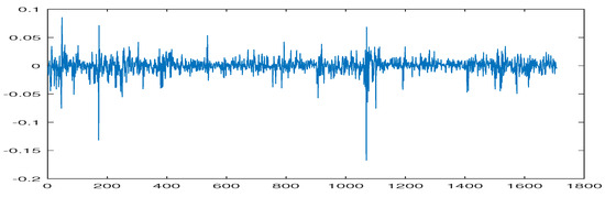
Figure 1.
Log returns of TASI for the period from 17 September 2014 to 5 June 2023.
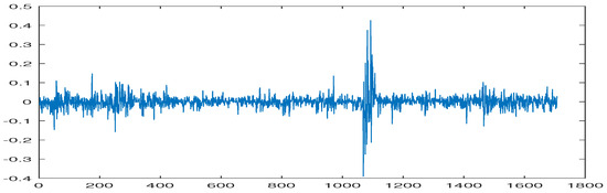
Figure 2.
Log returns of WTI index for the period from 17 September 2014 to 5 June 2023.
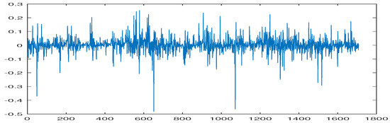
Figure 3.
Log returns of Bitcoin index for the period from 17 September 2014 to 5 June 2023.
5. Empirical Results
5.1. Results of Copulas Models
Table 1 provides descriptive statistics of the three returns, TASI, BTC, and WTI. The TASI returns present a mean of , indicating a slightly negative average return. The standard deviation is , suggesting a moderately high level of volatility in the TASI returns. The skewness value of indicates a highly skewed distribution, where the tail is longer on the left side. The kurtosis value of suggests a highly leptokurtic distribution. This means that there are more observations near the center and the tails are heavier than a normal distribution.

Table 1.
Descriptive statistics of the TASI, BTC, and WTI.
Bitcoin returns present a mean of , which means that the average value is positive and close to zero. The standard deviation of is relatively high, highlighting significant variability in returns. Thus, returns fluctuate substantially, implying the potential for both gains and losses. The skewness value of is very close to 0, suggesting a nearly symmetrical distribution. Returns are likely distributed evenly around the mean without strong tails. The kurtosis is , which means that the Bitcoin return distribution is moderately peaked and has heavy tails compared to a normal distribution.
The average return of indicates that WTI prices generally declined slightly over the analyzed period. The standard deviation of highlights significant price fluctuations, suggesting a volatile market with both potential gains and losses. The skewness value of reveals a distribution skewed towards negative returns. This means larger losses were more frequent than larger gains. The kurtosis is , indicating that the distribution of the returns of WTI crude oil is highly peaked and has heavy tails compared to a normal distribution.
Table 2 provides the estimation results of different copula families between Bitcoin and the TASI. The table presents the parameters for various copula families, including the lower tail dependence, upper tail dependence, LL, AIC, and BIC for each copula family. The estimation results provide insights into the dependence structure between Bitcoin and TASI returns, which is crucial for understanding the joint distribution of these two assets. By analyzing the parameters of different copula families, we can determine the most suitable copula for modeling the dependence between Bitcoin and TASI returns.
Table 2.
Parameter estimates of copulas models. Log Likelihood function (LL), AIC, and BIC of BTC–TASI returns.
The Student’s copula presents the lowest LL, AIC, and BIC. Thus, the optimal copula between TASI and BTC is the Student’s t copula, with a correlation of 0.0107 and 12.37 degrees of freedom. This low value of correlation indicates weak linear dependence between Bitcoin and TASI returns. The returns are not closely aligned, so they might not move together dramatically during market downturns. This weak correlation suggests potential diversification benefits from including both assets in a portfolio.
The degrees-of-freedom value of 12.37 indicates a moderately heavy-tailed distribution for the joint behavior of Bitcoin and TASI returns. It is more flexible than a normal distribution but not extremely heavy-tailed. It implies that risk models based on a Gaussian assumption might underestimate the likelihood of tail risks in this context. This is often relevant in finance, where moderate tail heaviness allows for capturing both regular and moderately extreme events. These heavy tails highlight the importance of considering tail risks when managing a portfolio that includes both Bitcoin and TASI assets.
The presence of a positive lower tail parameter of in the copula model suggests that, in the event of a notable negative return in Bitcoin, there is a moderate probability of observing a similarly significant negative event in the TASI. This indicates a certain degree of positive dependence in the lower tail, where extreme negative events in one asset are moderately correlated with extreme negative events in the other. Conversely, the positive upper tail parameter of implies that with the occurrence of a substantial positive return in Bitcoin, there is a moderate probability of encountering a significant positive event in the TASI. This signifies a positive dependence in the upper tail, indicating that extreme positive events in one asset are moderately correlated with extreme positive events in the other.
In Table 3, the optimal copula between the TASI and WTI crude oil is represented by a Student’s t copula with specific parameters. The correlation coefficient of 0.2013 indicates a mild positive linear relationship between the returns of the TASI and WTI crude oil, implying that, when one asset’s return increases, there is a tendency for the other to increase as well. The degrees-of-freedom parameter of 4.3676 suggests that the copula accommodates heavier tails in the joint distribution, allowing for a more flexible modeling of extreme events. Additionally, both lower and upper tail parameters of 0.1135 indicate a moderate level of positive tail dependence, suggesting that significant negative or positive events in one asset are moderately correlated with corresponding events in the other.
Table 3.
Parameter estimates of copulas models. Log Likelihood function (LL), AIC, and BIC of WTI–TASI returns.
In Table 4, the optimal copula between BTC and WTI crude oil is the Frank copula with a parameter of , which indicates that the joint dependence structure between these two assets is best represented by a copula that allows for both positive and negative dependencies without tail dependence. The positive dependence between BTC and WTI crude oil is indicated by the positive parameter value of , which suggests that these assets tend to move in the same direction. The magnitude of the parameter provides insights into the strength of the dependence. In this instance, the parameter value of implies a moderately strong positive dependence between BTC and WTI crude oil, reflecting a significant but not perfect association between the two assets.
Table 4.
Parameter estimates of copulas models. Log Likelihood function (LL), AIC, and BIC of BTC–WTI returns.
Figure 4 presents the Student’s copula density of the TASI and BTC. The concentration of higher density values towards the center suggests a higher probability of joint occurrences of median values of TASI and BTC returns, while the tails of the plot indicate the probabilities of extreme values occurring together. Figure 5 presents the graph of a Student’s copula illustrating the dependence structure between the TASI and WTI. The color gradient from blue to yellow indicates increasing density values. The peak of the graph suggests a higher density and thus a higher probability of joint occurrences around those particular values of TASI and WTI returns.
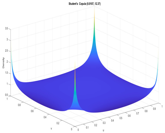
Figure 4.
Student’s copula density of the TASI and BTC.
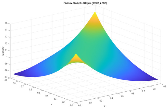
Figure 5.
Student’s copula density of the TASI and WTI.
A comparison of Figure 4 and Figure 5 shows that the parameters and the shapes of the copula densities are different, reflecting the distinct dependence structures between the TASI–BTC and TASI–WTI pairs. The degrees-of-freedom parameter is lower in Figure 5, which suggests a heavier tail and possibly more extreme joint behavior between TASI and WTI than between TASI and BTC. Figure 6 presents the Frank copula density of the BTC and WTI. This particular figure compares the density of the returns of BTC and WTI and could help investors to assess which asset has a greater likelihood of significant losses or gains in a short period. Understanding this information can help investors better manage their portfolio risk.
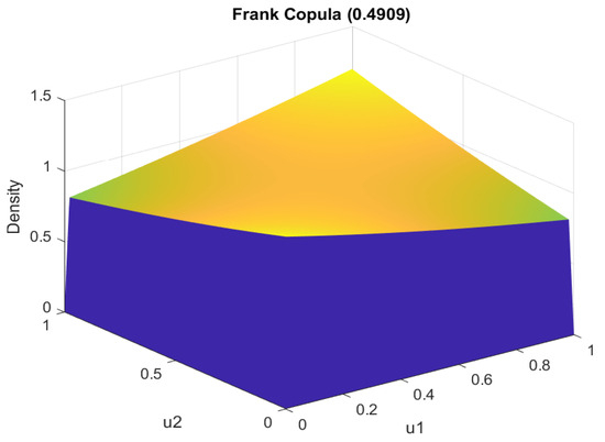
Figure 6.
Frank copula density of the BTC and WTI.
5.2. Results of LSTM Model
Figure 7, Figure 8 and Figure 9 present comparisons between the predicted and observed values for TASI, BTC, and WTI returns, accompanied by the calculated RMSE for each set of predictions. These visual comparisons suggest a strong alignment between the predicted trends and the actual market behaviors in instances where the actual returns decreased or the forecasts showed similar trends. Particularly notable is the LSTM model’s performance on TASI returns, where the predicted values closely mirror the actual returns. The BTC and WTI predictions also exhibit a high degree of accuracy. The RMSE values for these forecasts are notably low, with means of 0.014908 for TASI, 0.051661 for BTC, and 0.038728 for WTI, indicating precise model predictions.
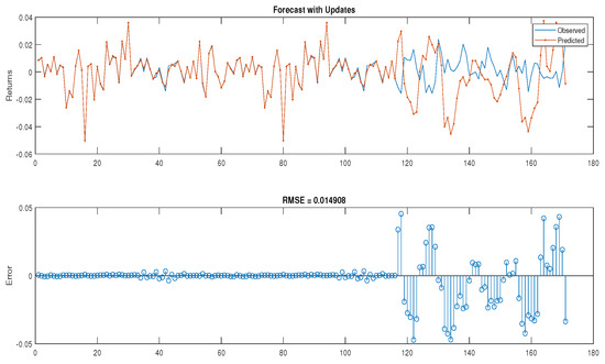
Figure 7.
Forecasted values with the test data of the TASI returns.
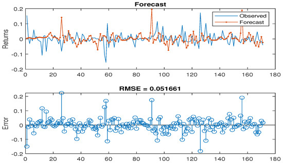
Figure 8.
Forecasted values with the test data of the BTC returns.
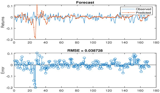
Figure 9.
Forecasted values with the test data of the WTI returns.
Further insights are provided by Figure 10, Figure 11 and Figure 12 which show the training and testing phases for the TASI, BTC, and WTI return models. The figures highlight the training data in blue and the testing data in orange. The consistency observed in the testing data reflects the patterns established during training, underscoring the neural network’s capability of effectively modeling the time-series data for the returns. This coherence between the trained and tested data points reinforces the conclusion that neural networks are a robust tool for modeling financial time series.
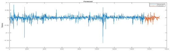
Figure 10.
The training TASI returns with the forecasted values.
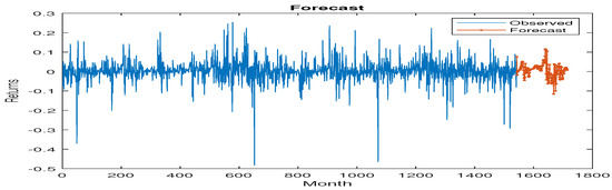
Figure 11.
The training BTC returns with the forecasted values.
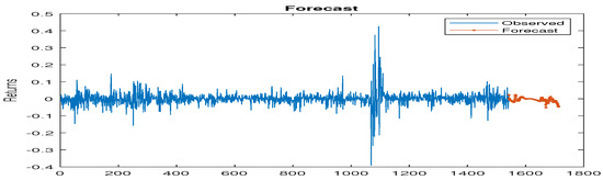
Figure 12.
The training WTI returns with the forecasted values.
5.3. Comparison between Copulas and LSTM Models
To evaluate the predictive performance of the copulas and LSTM models, we computed the RMSE, MAE, and MASE. Lower values of RMSE, MAE, and MASE indicate better predictive performance, reflecting the closeness of predicted values to the actual data observations. Table 5, Table 6 and Table 7 display the copula models’ accuracy in terms of RMSE, MAE, and MASE for the TASI, BTC, and WTI returns, and Table 8 displays the LSTM model’s RMSE, MAE, and MASE for the same returns.
Table 5.
RMSE, MAE, and MASE calculated from the prediction of the TASI and BTC.
Table 6.
RMSE, MAE, and MASE calculated from the prediction of the TASI and WTI.
Table 7.
RMSE, MAE, and MASE calculated from the prediction of the BTC and WTI returns.
Table 8.
RMSE, MAE, and MASE calculated from the prediction of the TASI, BTC and WTI returns with LSTM model.
Our results show the superior predictive power of LSTM models over copula-based approaches for predicting TASI, BTC, and WTI returns. The consistently lower RMSE, MAE, and MASE values achieved by the LSTM on all assets emphasize its ability to effectively capture the complex, non-linear dynamics of these financial time series. This better performance emphasizes the advantage of using a model that is able to learn complex temporal dependencies over methods that rely on static dependency structures. While the LSTM shows consistent improvements over copulas in predicting BTC and WTI, the MASE score for TASI (1.2), which indicates slightly worse performance than a naive forecast, is worth careful consideration. This result is likely due to the prevalence of near-zero returns in the TASI data, which can have a disproportionate effect on percentage error metrics such as MASE. However, the relatively low RMSE and MAE values for TASI suggest that the model’s predictions are still quite accurate in absolute terms. Overall, our study highlights the promising capabilities of LSTM models for financial forecasting while emphasizing the importance of understanding the data characteristics and using a combination of error metrics to effectively evaluate model performance.
6. Conclusions
The study employed two approaches, which are copula models and LSTM networks, as a way of examining the complex relationships between TASI, crude oil prices (WTI), and Bitcoin returns by emphasizing their mutual influences, interplays in investment decisions, and risk management. The empirical findings highlight the significance of tail dependencies in the TASI–BTC and TASI–WTI relationships. The Student’s t copula was identified as the most appropriate for capturing these dependencies. However, the BTC–WTI relationship exhibited a nonlinear correlation without tail dependence, which was best represented by the Frank copula.
Based on our results, we find that LSTMs perform better than copulas in the asset pairs of the study through lower RMSE, MAE, and MASE, which indicate superior prediction of asset returns. Combining LSTM networks with copula models to enhance financial time-series modeling and forecasting can help comprehend market dynamics for better investments. The integration of LSTM networks with copula models allows for capturing both temporal patterns and complex dependencies between assets. While LSTM networks excel at learning from sequential data, copula models are adept at modeling dependencies between different assets. This combined approach leverages the strengths of both methods, providing a more comprehensive understanding of market dynamics.
The results of this study indicate the critical importance of taking into account linear and nonlinear correlations, as well as dependencies, when examining the dynamics between distinct asset classes. In addition, the results highlight the significant effectiveness of LSTM networks in accurately predicting asset returns. These results underscore the potential for synergy between machine-learning methodologies and well-established econometric models, thus enhancing investment strategies and enhancing risk management practices within the evolving financial ecosystem.
Author Contributions
Conceptualization, S.A.A. and S.A.; methodology, S.A.A., S.A. and G.A.; software, S.A.A., S.A. and G.A.; formal analysis, S.A.A., S.A. and G.A.; investigation, S.A.A., S.A. and G.A.; data curation, S.A.A.; writing—original draft preparation, S.A.A., S.A. and G.A.; writing—review and editing, S.A.A., S.A. and G.A.; visualization, S.A.A., S.A. and G.A.; project administration, S.A.A. All authors have read and agreed to the published version of the manuscript.
Funding
This research received no external funding.
Data Availability Statement
The raw data supporting the conclusions of this article will be made available by the authors on request.
Conflicts of Interest
The authors declare no conflict of interest.
References
- Nakamoto, S. Bitcoin: A Peer-to-Peer Electronic Cash System; 2008. Available online: https://bitcoin.org/en/ (accessed on 15 April 2024).
- Kuziak, K.; Górka, J. Dependence Analysis for the Energy Sector Based on Energy ETFs. Energies 2023, 16, 1329. [Google Scholar] [CrossRef]
- Mo, B.; Meng, J.; Wang, G. Risk Dependence and Risk Spillovers Effect from Crude Oil on the Chinese Stock Market and Gold Market: Implications on Portfolio Management. Energies 2023, 16, 2141. [Google Scholar] [CrossRef]
- Alokley, S.A.; Albarrak, M.S. Clustering of extremes in financial returns: A study of developed and emerging markets. J. Risk Financ. Manag. 2020, 13, 141. [Google Scholar] [CrossRef]
- Cont, R. Empirical properties of asset returns: Stylized facts and statistical issues. Quant. Financ. 2001, 1, 223. [Google Scholar] [CrossRef]
- Mokni, K.; Youssef, M. Measuring persistence of dependence between crude oil prices and GCC stock markets: A copula approach. Q. Rev. Econ. Financ. 2019, 72, 14–33. [Google Scholar] [CrossRef]
- Awartani, B.; Maghyereh, A.I. Dynamic spillovers between oil and stock markets in the Gulf Cooperation Council Countries. Energy Econ. 2013, 36, 28–42. [Google Scholar] [CrossRef]
- Naifar, N.; Al Dohaiman, M.S. Nonlinear analysis among crude oil prices, stock markets’ return and macroeconomic variables. Int. Rev. Econ. Financ. 2013, 27, 416–431. [Google Scholar] [CrossRef]
- Mohanty, S.K.; Nandha, M.; Turkistani, A.Q.; Alaitani, M.Y. Oil price movements and stock market returns: Evidence from Gulf Cooperation Council (GCC) countries. Glob. Financ. J. 2011, 22, 42–55. [Google Scholar] [CrossRef]
- Boubaker, H.; Sghaier, N. Instability and dependence structure between oil prices and GCC stock markets. Energy Stud. Rev. 2013, 20, 50–65. [Google Scholar] [CrossRef][Green Version]
- Syuhada, K.; Suprijanto, D.; Hakim, A. Comparing gold’s and Bitcoin’s safe-haven roles against energy commodities during the COVID-19 outbreak: A vine copula approach. Financ. Res. Lett. 2022, 46, 102471. [Google Scholar] [CrossRef]
- Mzoughi, H.; Ghabri, Y.; Guesmi, K. Crude oil, crypto-assets and dependence: The impact of the COVID-19 pandemic. Int. J. Energy Sect. Manag. 2023, 17, 552–568. [Google Scholar] [CrossRef]
- Jin, F.; Li, J.; Li, G. Modeling the linkages between Bitcoin, gold, dollar, crude oil, and stock markets: A GARCH-EVT-copula approach. Discret. Dyn. Nat. Soc. 2022, 2022, 8901180. [Google Scholar] [CrossRef]
- Garcia-Jorcano, L.; Benito, S. Studying the properties of the Bitcoin as a diversifying and hedging asset through a copula analysis: Constant and time-varying. Res. Int. Bus. Financ. 2020, 54, 101300. [Google Scholar] [CrossRef] [PubMed]
- Wang, H.; Wang, X.; Yin, S.; Ji, H. The asymmetric contagion effect between stock market and cryptocurrency market. Financ. Res. Lett. 2022, 46, 102345. [Google Scholar] [CrossRef]
- Hochreiter, S.; Schmidhuber, J. Long short-term memory. Neural Comput. 1997, 9, 1735–1780. [Google Scholar] [CrossRef] [PubMed]
- Gers, F.A.; Schmidhuber, J.; Cummins, F. Learning to forget: Continual prediction with LSTM. Neural Comput. 2000, 12, 2451–2471. [Google Scholar] [CrossRef] [PubMed]
- Graves, A.; Schmidhuber, J. Framewise phoneme classification with bidirectional LSTM and other neural network architectures. Neural Netw. 2005, 18, 602–610. [Google Scholar] [CrossRef] [PubMed]
- Fischer, T.; Krauss, C. Deep learning with long short-term memory networks for financial market predictions. Eur. J. Oper. Res. 2018, 270, 654–669. [Google Scholar] [CrossRef]
- Zhang, K.; Hong, M. Forecasting crude oil price using LSTM neural networks. Data Sci. Financ. Econ. 2022, 2, 163–180. [Google Scholar] [CrossRef]
- Latif, N.; Selvam, J.D.; Kapse, M.; Sharma, V.; Mahajan, V. Comparative performance of LSTM and ARIMA for the short-term prediction of bitcoin prices. Australas. Account. Bus. Financ. J. 2023, 17, 256–276. [Google Scholar] [CrossRef]
- Niu, J.; Li, S.; Xu, W.; Dong, F.; Huang, F.; Qiu, H. An efficient LSTM network for predicting the tailing and multi-peaked breakthrough curves. J. Hydrol. 2023, 624, 129914. [Google Scholar] [CrossRef]
- Alasiri, R.A.; Qahmash, A. Analysis and Forecasting of Saudi Stock Market Using Time Series Algorithms. In Proceedings of the 2023 3rd International Conference on Computing and Information Technology (ICCIT), Tabuk, Saudi Arabia, 10–11 May 2023; pp. 340–347. [Google Scholar]
- Pratas, T.E.; Ramos, F.R.; Rubio, L. Forecasting bitcoin volatility: Exploring the potential of deep learning. Eurasian Econ. Rev. 2023, 13, 285–305. [Google Scholar] [CrossRef]
- Hua, Y. Bitcoin price prediction using ARIMA and LSTM. In E3S Web of Conferences, Proceedings of the 2020 International Symposium on Energy, Environmental Science and Engineering (ISEESE 2020), Chongqing, China, 20–22 November 2020; EDP Sciences: Les Ulis, France, 2020; Volume 218, p. 01050. [Google Scholar]
- Aditya Pai, B.; Devareddy, L.; Hegde, S.; Ramya, B. A time series cryptocurrency price prediction using LSTM. In Emerging Research in Computing, Information, Communication and Applications: ERCICA 2020; Springer: Singapore, 2022; Volume 2, pp. 653–662. [Google Scholar]
- Ateeq, K.; Khan, M.A. A Mechanism for Bitcoin Price Forecasting using Deep Learning. Int. J. Adv. Comput. Sci. Appl. 2023, 14, 441–448. [Google Scholar] [CrossRef]
- Mohammed, S. The Validity of Using Technical Indicators When forecasting Stock Prices Using Deep Learning Models: Empirical Evidence Using Saudi Stocks. In Proceedings of the 2022 14th International Conference on Computational Intelligence and Communication Networks (CICN), Al-Khobar, Saudi Arabia, 4–6 December 2022; pp. 520–524. [Google Scholar]
- Koo, E.; Kim, G. Centralized decomposition approach in LSTM for Bitcoin price prediction. Expert Syst. Appl. 2024, 237, 121401. [Google Scholar] [CrossRef]
- Karahyla, J.K.; Sharma, N.; Chamoli, S.; Shirgire, A.; Kant, R.; Chauhan, A. Predicting Price Direction of Bitcoin based on Hybrid Model of LSTM and Dense Neural Network Approach. In Proceedings of the 2023 4th International Conference on Electronics and Sustainable Communication Systems (ICESC), Coimbatore, India, 6–8 July 2023; pp. 953–958. [Google Scholar]
- Sklar, A. Distribution Functions of n Dimensions and Margins; Institute of Statistics of the University of Paris: Paris, France, 1959; Volume 8, p. 31. [Google Scholar]
- Nelsen, R.B. An Introduction to Copulas, 2nd ed.; Springer: New York, NY, USA, 2006. [Google Scholar]
Disclaimer/Publisher’s Note: The statements, opinions and data contained in all publications are solely those of the individual author(s) and contributor(s) and not of MDPI and/or the editor(s). MDPI and/or the editor(s) disclaim responsibility for any injury to people or property resulting from any ideas, methods, instructions or products referred to in the content. |
© 2024 by the authors. Licensee MDPI, Basel, Switzerland. This article is an open access article distributed under the terms and conditions of the Creative Commons Attribution (CC BY) license (https://creativecommons.org/licenses/by/4.0/).