Article

A Contoured Controller Bode-Based Iterative Tuning Method for Multi-Band Power System Stabilizers

1
School of Electrical Engineering, Zhejiang University, Hangzhou 310027, China
2
Hangzhou Power Supply Company, State Grid Zhejiang Electric Power Co., Ltd., Hangzhou 310027, China
*
Author to whom correspondence should be addressed.
Energies 2024, 17(13), 3243; https://doi.org/10.3390/en17133243
Submission received: 23 May 2024 / Revised: 16 June 2024 / Accepted: 28 June 2024 / Published: 1 July 2024
(This article belongs to the Topic Power System Dynamics and Stability)

Abstract

:
An iterative tuning method for multi-band power system stabilizers is proposed, which utilizes the contoured controller Bode (CCBode) plot. The typical multi-band power system stabilizer, PSS4B, is conceptualized as a series connection of two filters: a band-pass filter and a phase compensator. The tuning process involves a space searching approach for the phase compensator to ensure its phase–frequency response remains within acceptable bounds. Subsequently, the CCBode plot is employed to adjust the magnitude–frequency response of the band-pass filter, thereby enhancing stability performance across a broad frequency range. The method proposed can be applied to the parameter design of the multi-band power system stabilizer PSS4B in the power system to suppress the low-frequency oscillations of the local mode and inter-regional mode in the system. The effectiveness of this proposed method is demonstrated through case studies of the four -machine/two-area system and the North China Power Grid.

1. Introduction

The mechanism of low-frequency oscillation in power systems involves the system oscillating near the steady-state operating point after a disturbance due to the inertial response of synchronous generators. This can lead to increased amplitude oscillations and a potential loss of synchronization. Low-frequency oscillation is an inherent issue in synchronous generator operation and has caused numerous incidents globally. For example, in 1996, a severe blackout in the western United States was attributed to low-frequency oscillation. Similarly, interconnected power grids in North China, Central China, and Northeast China have experienced low-frequency oscillations [1,2,3]. Particularly in the North China Power Grid, the damping ratio of regional oscillations has been declining since 2009, frequently triggering low-frequency oscillations after accidents, thereby constraining inter-provincial power transmission [4]. Power system stabilizers (PSSs) are recognized as one of the most effective methods to suppress low-frequency oscillations, among which the multi-band power system stabilizer PSS4B is more flexible thus has gained attention as a potential solution [5,6].
Compared to the widely used single-band power system stabilizer PSS2B, PSS4B incorporates three frequency bands that can, respectively, compensate the phase lag of different modes. Previous studies [7,8] indicate that the PSS4B outperforms the PSS2B in damping multiple modes due to its higher degrees of freedom, which, however, bring challenges to the parameter tuning of PSS4B.
The tuning process for PSS parameters remains an unsolved fixed-order controller design challenge within the control filed [9,10], and numerous heuristic approaches have been proposed. Many approaches rely on first-order approximations of the dominant eigenvalues [2,8,11,12,13]. Frequently, eigenvalue-based results are incorporated into an optimization model to yield more systematic solutions [3,14,15].
The most famous PSS tuning method is the so-called ideal phase curve method, which is an approach that is widely used in industry [16,17,18,19,20]. The shortcoming of this method is obvious, as it does not take the PSS magnitude–frequency characteristic into account and thus causes difficulties in PSS gain tuning. It is well recognized that one PSS has a critical gain, above which the instability of the so-called “exciter mode” occurs. As a rule of thumb, PSS gains are often set to one-third of the critical gain [21]. The existing method has a significant shortcoming: it separates the amplitude–frequency characteristic and phase–frequency characteristic of the PSS during the setting process. This separation makes it impossible to accurately measure the PSS’s contribution to the stability margin and to ensure that the designed PSS parameters provide maximum damping for the oscillation mode. To address this issue, a contoured controller Bode-based iterative tuning method is proposed for the parameter tuning of PSS4Bs.
This paper first reviews the symmetrical approach to PSS4B parameter tuning, which promotes the practical application of PSS4B at the expense of reducing control freedom and does not discuss how to optimize the amplitude–frequency characteristics. Therefore, it has inadequacy in providing enough damping for local modes. To solve this problem, this paper proposes a revised PSS4B model with enhanced phase compensation, and an iterative design method is introduced based on this model, leveraging the contour controller Bode (CCBode) plot, which offers clear stability margins and considers the damping ratio. This method is based on two tuning tools: the space searching approach for tuning the appended phase compensation blocks, and the CCBode plot for tuning the band-pass filters to design PSS4B in an iterative manner. The advantage of the method is that both inter-area and local modes avoid the instability of the exciter mode, ensuring that the system can provide sufficient damping in the full frequency band of low-frequency oscillations, and has good engineering application prospects. The effectiveness of the proposed method is verified by the classic four-machine/two-area system and the North China Power Grid.

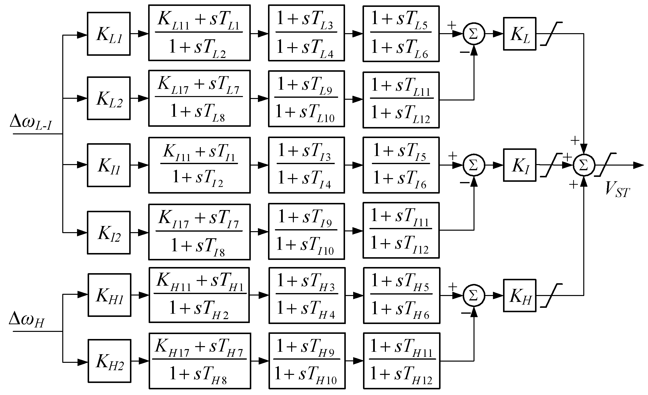
2. Revised Model of PSS4B

2.1. The Limitation of the Symmetrical Approach

The general structure of the PSS4B is shown in Figure 1. The widely used symmetrical approach uses only the first block in each branch and synthesize the pairs of lead–lag blocks into three symmetrical band-pass filters with center frequencies FL, FI, and FH and gains KL, KI, and KH [6].
In Figure 1, s is the Laplace operator; ΔωLI is the input of the low- and medium-frequency branch, which is often the speed of generator; ΔωH is the input of high frequency branch, which is often the active power of the generator; VST is the output signal of PSS4B, where each T represents a time constant.
The parameters are derived from the following equations when taking the high-frequency band as an example:
K H 11 = K H 17 = 1 ( lead - lag blocks ) T H 2 = T H 7 = 1 / ( 2 π F H R ) T H 1 = T H 2 / R T H 8 = T H 7 × R K H 1 = K H 2 = ( R 2 + R ) / ( R 2 2 R + 1 ) .
In Equation (1), R is the constant ratio, which is often set to 1.2.
Therefore, the transfer function of the high band GHn(s) is given:
G H n ( s ) = K H ( R 2 + R ) s R ( 2 π F H R + s ) ( 2 π F H + R s ) .
The transfer function given in (2) can be viewed as a band-pass filter with a center frequency FH. Compared with the complex combination of the original lead–lag blocks, the simplified PSS4B model has a clear physical meaning.
As the gains KL, KI, and KH for the three band-pass filters are tuned independently, the PSS4B stabilizer enjoys many more degrees of freedom than the PSS2B stabilizer, which has only one gain parameter. This feature allows for the PSS4B to produce a flexible magnitude–frequency characteristic that not only offers sufficient damping to electromechanical oscillation modes, but also prevents the stabilizer gain from reaching too high in the high frequency range.
However, a PSS4B stabilizer designed using the above symmetrical parameter approach cannot provide enough phase compensation. To explain it, substitute s = in (2) and then notice the following:
G H n ( j ω ) = 90 tan 1 ω ( 1 + R ) R ( 2 π F H ω 2 / 2 π F H ) ,
which is a monotonically decreasing function with a maximum value of 90° at ω = 0. Therefore, the total phase compensation provided by a PSS4B is limited:
G P S S 4 B n ( j ω ) = G L n ( j ω ) + G I n ( j ω ) + G H n ( j ω ) max G L n ( j ω ) , G I n ( j ω ) , G H n ( j ω ) = 90 ° ,
which is no greater than each of its frequency band can supply. The experience in the North China system shows that a PSS is sometimes required to provide a phase compensation over 100° to damp the local modes. Therefore, the PSS4B tuned using the symmetrical setting approach does not meet this requirement.

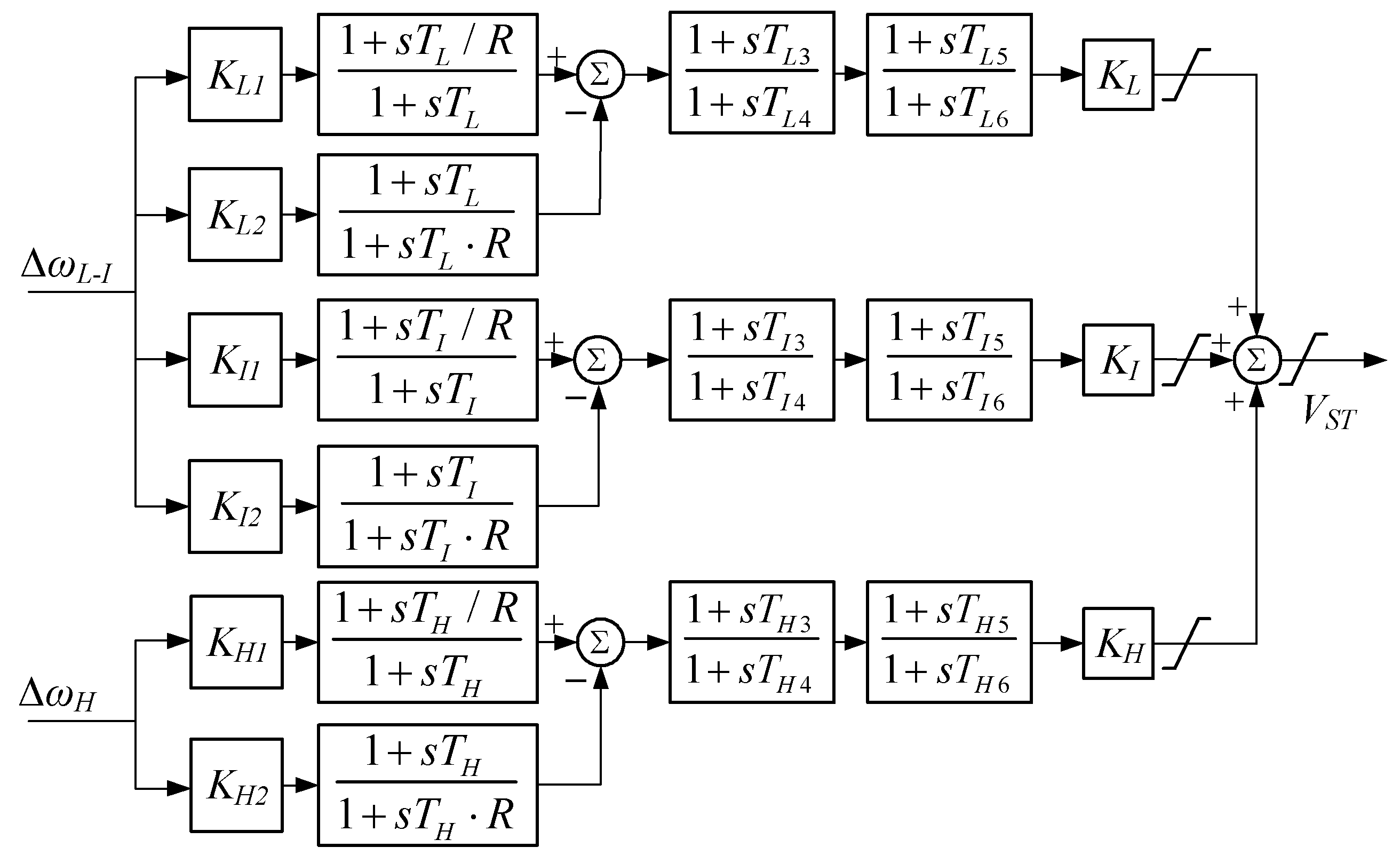
2.2. The Revised Model of PSS4B

Such a lack of enough phase compensation can be overcome by appending two additional lead–lag blocks to each band, as shown in Figure 2.
Here, we recommend a parameter setting principle for these additional blocks so that they fit in with the symmetrical setting approach. Take the high-frequency band as an example; we set the parameters as follows:
T H 3 = T H 9 , T H 4 = T H 10 , T H 5 = T H 11 , T H 6 = T H 12 ,
then, the transfer function for the high band GH(s) becomes as follows:
G H ( s ) = G H n ( s ) 1 + s T H 3 1 + s T H 4 1 + s T H 5 1 + s T H 6 .
For each lead–lag block, e.g., G() = (1 + jωTH3)/(1 + jωTH4), it can be easily proved that the maximum phase ∠G(m) is 90° at ω m = 1 / T H 3 T H 4 . Thus, the two lead–lag blocks in (6) provide a phase lead up to 180°, and so do the ones in the other two bands. With this approach, the PSS4B stabilizer enjoys more degrees of freedom in achieving a precise phase–frequency characteristic that covers a wide spectrum of frequencies.

3. Iterative Design of PSS4B Stabilizer

The revised model of PSS4B in Section 2 raises the upper limit of the phase compensation while preserving the original advantages of the symmetrical approach. However, compared with conventional PSSs, the PSS4B stabilizer has a large number of parameters, which compounds the tuning process. In this section, we first introduce two tuning tools: the space searching approach for tuning the appended phase compensation blocks, and the CCBode plot for tuning the band-pass filters. We then show how to use these tools to design PSS4B in an iterative manner.

3.1. Space Searching Approach

Suppose a fixed-structure controller is given:
C ( s , d ) = l = 0 n β l s l i = 0 m α i s i ,
where αi and βl (for i = 0,, m and l = 0,…, n) are the parameters of the controller. Let d = [α0,…, αm, β0,…, βn] be the parameter vector. The task is to find a vector d such that the closed-loop system meets various engineering requirements.
The idea of the suggested iterative design is illustrated in Figure 3, where C(s, d) is the controller of which the parameters are to be sought, and Cr(s) is the desired reference controller. For now, let us suppose the frequency response of the reference controller Cr(s) is known. Given a parameter space, which is a hyper-rectangular domain, for the controller D = {d | αi ∈ [αi, αi+], i = 0,…, m, βl ∈ [βl, βl+], l = 0,…, n}, where αi and αi+ are the upper and lower bounds for parameter αi, and βl and βl+ are the upper and lower bounds for parameter βl, our goal is to find a feasible d D so that the frequency response error e = C(, d) − Cr() is acceptable.
In Figure 3, y is the input of the controller, u is the output of the controller, ur is the desired output of the controller, and e is the error of the output.
Consider a set of distinct frequencies [ω1, ω2,…, ωN], where ω1 is the lowest frequency, and ωN is the highest. The desired controller can be defined as follows:
C r ( j ω Ω ) = C r ( j ω Ω ) C r ( j ω Ω ) , Ω = 1 , , N
where |Cr(Ω)| and ∠Cr(Ω) are the desired magnitude and phase–frequency responses of the controller Cr(s) at frequency ωΩ, Ω = 1,…, N. Note that the desired reference controller Cr(s) need not have a closed-form expression—it can be a set of measured frequency-dependent data points, that is, this method is data-driven.
Similarly, the actual controller C(s, d) is expressed as
C ( j ω Ω , d ) = C r ( j ω Ω , d ) C ( j ω Ω , d ) , Ω = 1 , , N
where |C(Ω, d)| and ∠C(Ω, d) are the magnitude and phase–frequency responses of C(s) at frequency ωΩ, Ω = 1,…, N.
The error between the actual frequency response C(, d) and the desired frequency response Cr() is defined as follows:
e ( ω Ω , d ) = C r ( ω Ω ) C ( ω Ω , d ) , Ω = 1 , , N
and
e ( ω Ω , d ) = C r ( ω Ω ) C ( ω Ω , d ) , Ω = 1 , , N
where |e(ωΩ, d)| is the magnitude error and ∠e(ωΩ, d) is the phase error at frequency ωΩ, Ω = 1,…, N.
Now, the control design problem is formulated as a frequency domain curve-fitting problem as follows: find a feasible parameter vector d D so that for each of the frequencies of concern ωΩ, Ω = 1,…, N, both the magnitude and phase errors remain bounded within their respective limits.
A l ( ω Ω ) e ( ω Ω , d ) A u ( ω Ω ) θ l ( ω Ω ) e ( ω Ω , d ) θ u ( ω Ω )
The upper and lower bounds for the magnitude and phase errors, Al(ωΩ), Au(ωΩ), θl(ωΩ), and θu(ωΩ), Ω = 1,…, N, are chosen small enough to ensure that the actual frequency response C(Ω, d) is close enough to the desired response Cr(Ω) at any of the frequencies ωΩ, Ω = 1,…, N.
The above curve-fitting problem can be solved using several algorithms. In this work, we tested three methods: a grid search algorithm recently presented in [22], a Monte Carlo algorithm we developed in [23], and a global optimization method described in [24]; all three methods worked well.
It remains to determine the reference controller response Cr(). There are basically two approaches. In the first approach, specify the desired reference controller response |Cr()|, ∠Cr() using a CCBode, and solve (12) for the parameters of the controller.
To describe the second approach, let us define a complex matrix HEX:
H E X = K 2 K 6 + K A 1 ( j ω T A + I ) ( j ω T d 0 + K 3 ) 1 ,
where K2, K3, and K6 are system coefficient matrices [2]; I is an identity matrix; TA is a diagonal matrix of exciter time constants; and Td0 is a diagonal matrix with machine constants. Notice that the phase lag of the excitation system of the k-th generator is equal to HEX(k,k) [8]. This phase lag can be either computed [19] or measured onsite [21].
In the second approach, first determine the parameters of the band-pass filters using the CCBode plot, then let the reference phase response ∠Cr() be equal to the phase lag of the excitation system. To find the parameters of the phase compensation filters, let d = [Ti3, Ti4, Ti5, Ti6], i ∈ {L, I, H}. Solve problem (12), obtaining all the parameters of a PSS4B.
The second approach is adopted in this work, as it is most consistent with the practice widely accepted in the industry. In what follows, we will illustrate how to determine the parameters of the band-pass filters using the CCBode plots.

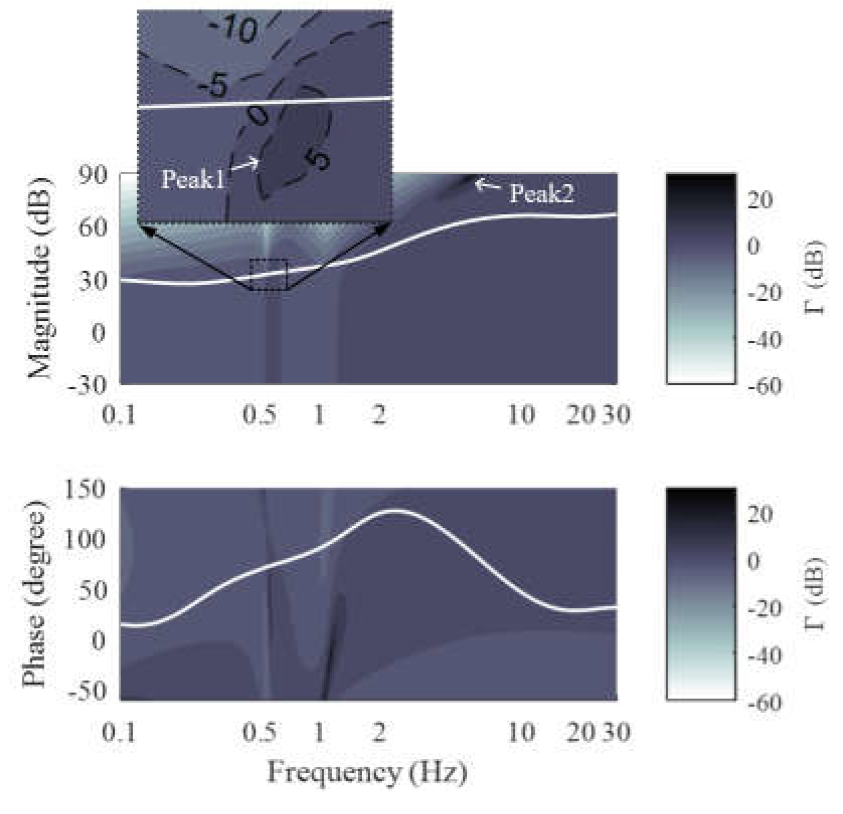
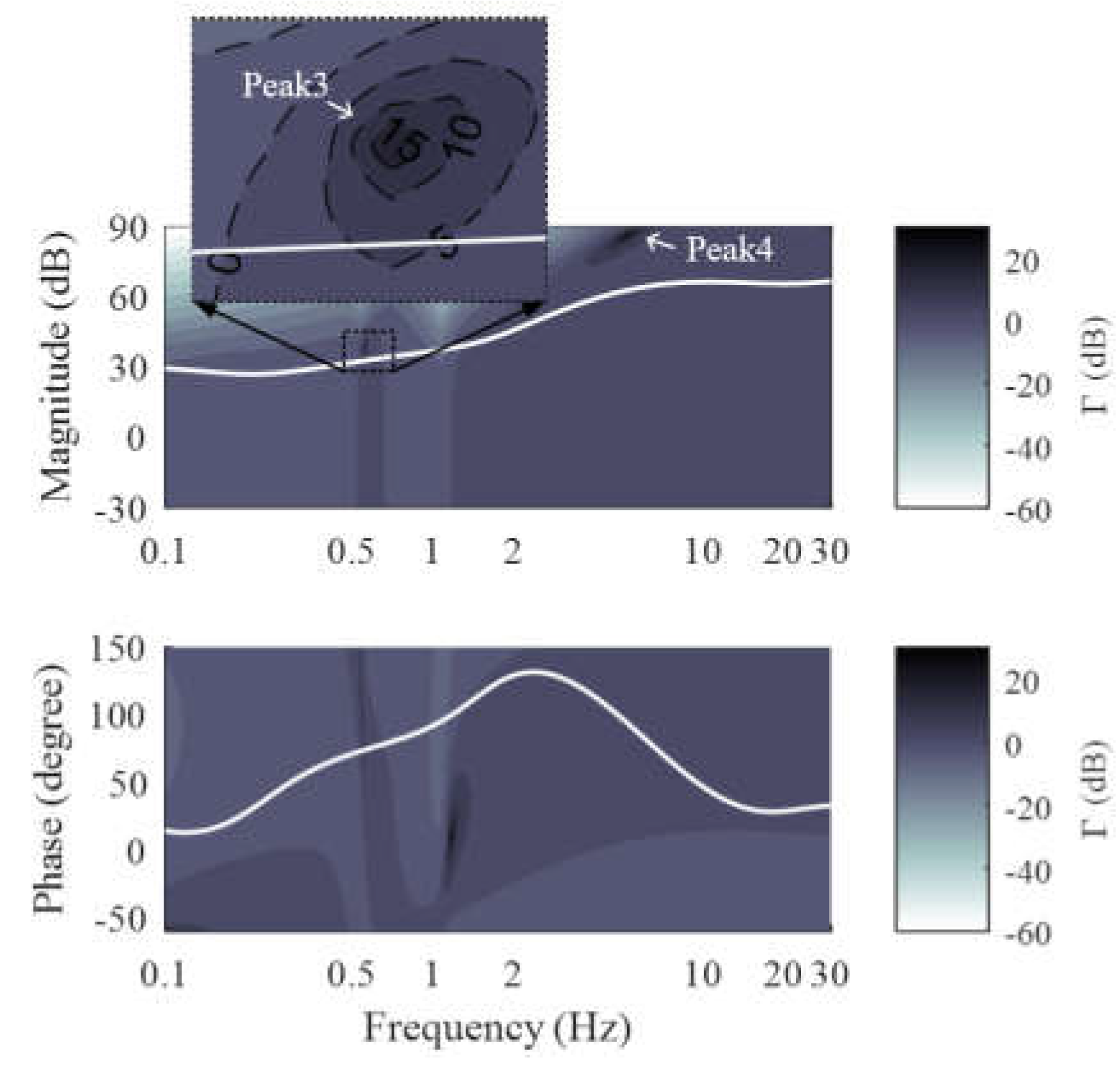
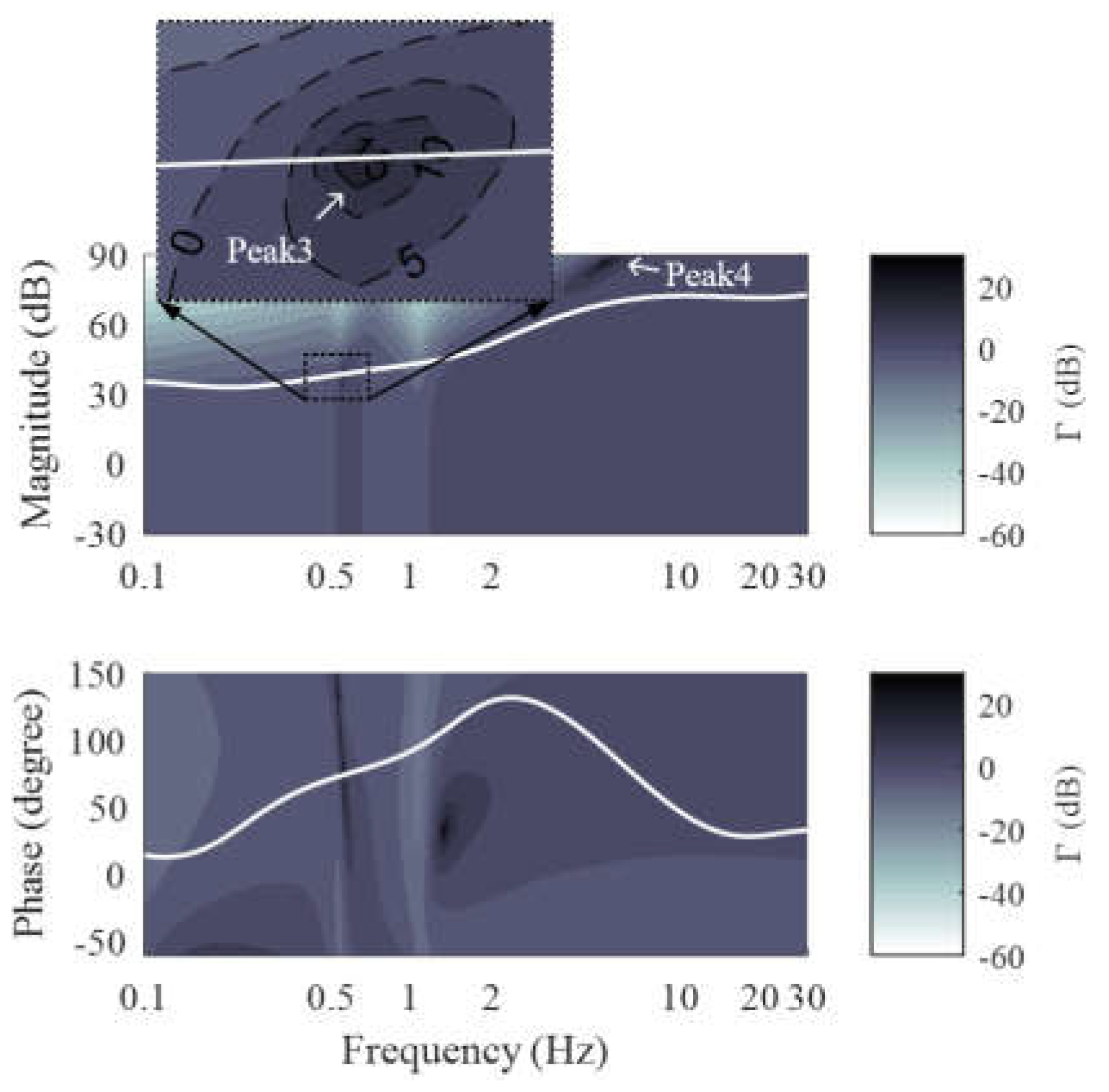
3.2. Contoured Controller Bode Plot

Compared with the classic Bode plot, a CCBode plot [25,26] gives the frequency characteristic of the controller despite the system. The advantage of the CCBode is that it illustrates the contours of the performance index Γ(ω). The values of Γ(ω) indicate the stability margin of the system, a weighted average of stability margin, or other desired performance indices, say, output energy [27]. In this work, only stability margin is considered.

3.2.1. Performance Index
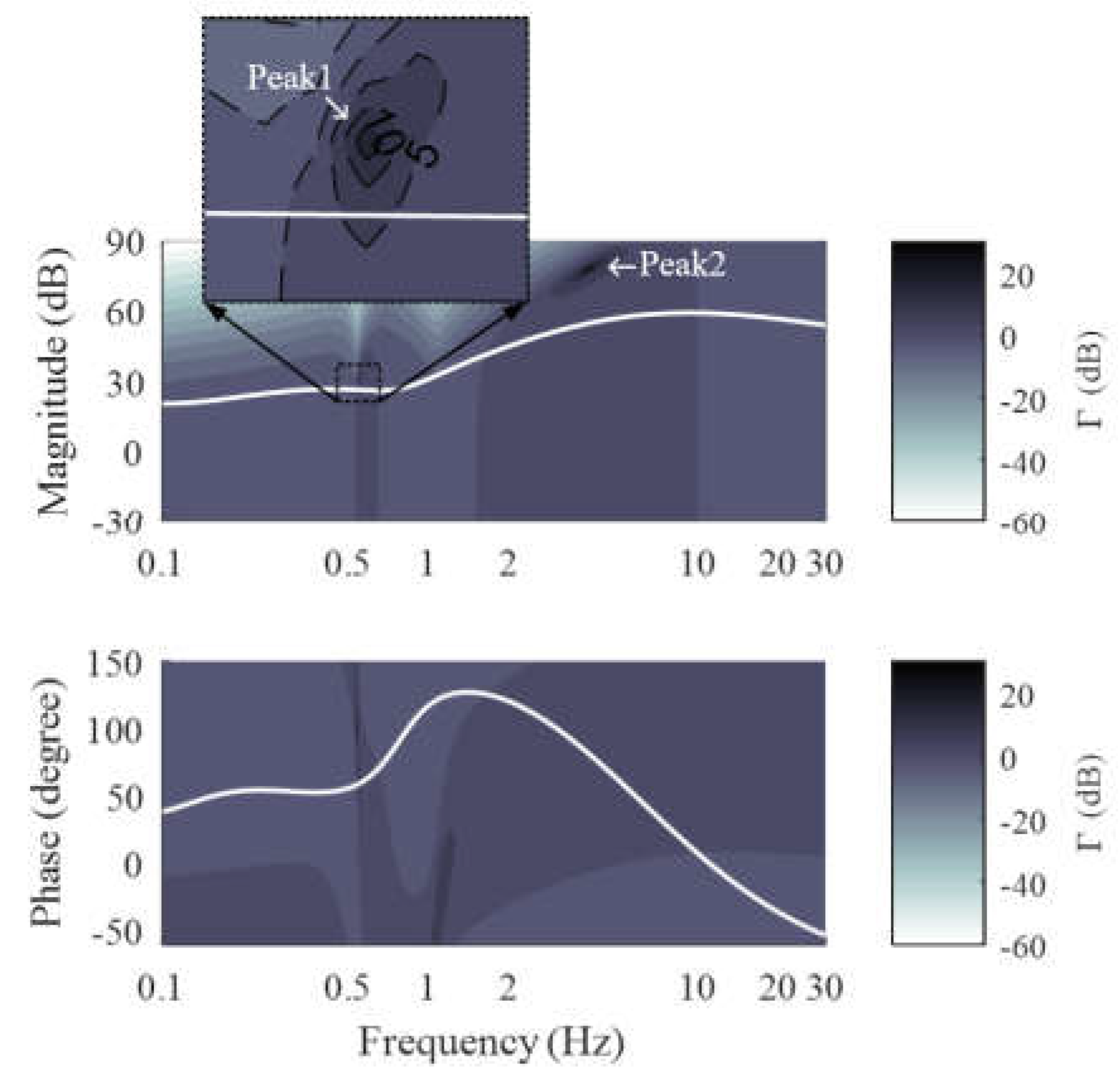
Figure 4 shows a PSS installed at the k-th generator of a multi-machine power system, where C() is the controller, and ωk and Vrefk are the frequency and the voltage reference of the generator, respectively. The output signal VSTk of the controller is applied to the reference voltage of the excitation. The multi-machine system is described by its frequency response G(). The open-loop transfer function can be defined Lo(s) as follows:
L o ( s ) = C ( s ) G ( s ) ,
Then, the characteristic equation of the closed-loop system is as follows:
1 + L o ( s ) = 0 .
According to Nyquist stability criterion, the distance |1 + Lo()| between Lo() and the critical point (−1, j0) can be viewed as a stability margin of the system.
From a control point of view, the objective of a PSS is to shift the dominant eigenvalues to the left. Let the order of the open-loop system be n; then, G(s) be can expressed by the following partial fraction expansion:
G ( s ) = R 1 s λ 1 + + R n s λ n ,
where R1,…, Rn are the residues. Consider λp = σp + jωp as an eigenvalue of the open-loop system; it follows that the eigenvalue shift introduced by a PSS has the following first-order approximation formula [10]:
Δ λ p R p C ( s ) s = λ p = R p L o ( s ) s = λ p G ( s ) s = λ p R p L o ( j ω p ) G ( j ω p ) .
Since residue Rp and open-loop frequency response G(p) are fixed, the magnitude of 1 + Lo(p) is therefore a clear measure of stability margin. In particular, if λp is purely imaginary, then σp = 0 and |1 + Lo()| = 0. When λp is shifted to the left, |1 + Lo()| varies in a pattern determined by λp’s point of departure. If λp is initially stable, the distance |1 + Lo()| will increase at frequencies around ωp; if λp is initially unstable, then |1 + Lo()| will decrease at first, until it reaches 0; then, it will increase.
Therefore, define the performance index Γ(ω) as the reciprocal of the distance between Lo() and (−1, j0):
Γ ( ω ) : = 1 1 + L o ( j ω ) .
Thus, the values of Γ(ω) at frequencies around ωp indicate the relative stability of λp: if λp is initially stable, then the lower values of Γ(ω) at frequencies around ωp indicate a more stable λp; if λp is initially unstable, then a more stable λp requires that Γ(ω) increases at first, until Γ(ωp) reaches +∞ and then decreases.

3.2.2. CCBode Plot

To construct a CCBode plot, it is first required to obtain the frequency responses of the open-loop system and the controller, G() and C(). The structure of a controller like a PSS is often not complicated, so the magnitude–frequency response |C()| and phase–frequency response ∠C() can be easily calculated by a sweep over ω.
Two methods can be used to obtain the frequency response G(): from a field measurement, or from the data of an operating condition. As for the latter option, it is usually derived from the state-space model of the system.
G ( j ω ) = c T ( j ω I A ) 1 b .
where A is the state-space matrix, and b and c are input and output vectors. However, the order of a large-scale power system model can be very high. If we tried to derive G() by a sweep over ω using its state-space model, the computational cost would be huge. To compute G() efficiently, we apply the sparsity method described in [28]. Consider a power system given by its differential algebraic equation (DAE) model:
x ˙ 0 = J 1 J 2 J 3 J 4 J n x + n v x v + b u , y = c T x v ,
where x is the nx-dimensional state-variable vector, v is the nv-dimensional algebraic-variable vector, u is the algebraic variable representing the input, and y is the algebraic variable representing the output. Then, we have
G ( j ω ) = c T j ω I n x 0 n v J 1 b .
This method makes use of the sparsity of the Jacobian matrix J, therefore producing solutions of the magnitude–frequency response |G()| and phase–frequency response ∠G() at a low computational cost.
Now we are in a position to derive the CCBode plot. When designing a controller for a plant, notice that the plant frequency response G() is given:
Γ ( ω ) = 1 1 + L o ( j ω ) = 1 [ 1 + L o ( j ω ) ] [ 1 + L *   o ( j ω ) ] = 1 1 2 G ( j ω ) C ( j ω ) cos G ( j ω ) + C ( j ω ) + G ( j ω ) 2 C ( j ω ) 2 .
When determining the CCBode magnitude plot, the controller phase ∠C() needs to be fixed. Now, the magnitude index Γmag is a function of frequency ω and controller gain K:
Γ m a g ( ω , K ) = 1 1 2 G ( j ω ) K cos G ( j ω ) + C ( j ω ) + G ( j ω ) 2 K 2 .
The contours of the magnitude function Γmag(ω, K) can now be easily constructed using graphical tools. To build a CCBode phase plot, fix the controller magnitude |C()|. The phase performance index Γphase becomes a function of frequency ω and controller phase φ:
Γ p h a s e ( ω , φ ) = 1 1 2 G ( j ω ) C ( j ω ) cos G ( j ω ) + φ + G ( j ω ) 2 C ( j ω ) 2 .
Again, the contours of the phase function Γphase(ω, φ) can be easily obtained. With the CCBode plot, we can adjust |C(ω)| and ∠C(ω) by tuning the parameters of the PSS so that Γ(ω) decreases at the frequencies of concern, thus improving the damping of the corresponding modes.

3.2.3. CCBode Plot Using Generalized Frequency

The afore-described CCBode plot is based on the classic Nyquist stability criterion, which states the condition that a controller shall satisfy in order to keep eigenvalues from crossing the imaginary axis. This is known as Hurwitz stability. In practice, however, regulations often require that the minimum damping ratio should not fall less than 3% [19]. This is the so-called D-stability. In this section, we extend the previous solution to deal with this practical issue.
An analogous Nyquist-type stability criterion exists for D-stability [29]: to determine the number of poles/zeros inside an arbitrary, bounded, symmetrical region in the complex plane, we only need to replace s = in the classic Nyquist theorem with the so-called generalized frequency s = σ + when plotting the Nyquist diagram (see Figure 5).
Let ζ be the desired damping ratio; the definition of the generalized frequency s = σ + is as follows:
s ( ω , ζ ) = σ ( ω , ζ ) + j ω = ( ζ 1 ζ 2 + j ) ω , ω [ 0 , ) .
In (25), σ(ω, ζ) is the real part of s(ω, ζ) determined by the frequency ω of concern and the damping ratio ζ of this mode.
To construct a CCBode plot with a given damping ratio ζ, we follow the same process described in the previous subsection, except that this time, generalized frequency s(ω, ζ) is used in the calculation of frequency responses G(s(ω, ζ)) and C(s(ω, ζ)). Obviously, if 1 + Lo(s(ω, ζ)) = 0, an eigenvalue passes through the stability boundary. Therefore, the performance index Γ(ω, ζ) using generalized frequency is also a useful indication of stability margin:
Γ ( ω , ζ ) : = 1 1 + L o ( s ( ω , ζ ) ) .
Compared with the classic Bode plot, the CCBode plot directly shows the frequency response of the controller, which simplifies the controller tuning process.

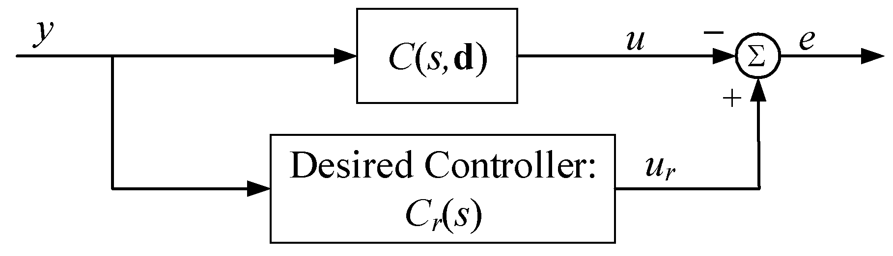
3.3. Iterative Design Approach

We first assign typical values to the band-pass filter parameters KL, KI, KH, FL, FI, FH, and R, and calculate the parameters of the appended phase compensation blocks Ti3, Ti4, Ti5, and Ti6, i ∈ {L, I, H}, by the space searching approach.
Then, we calculate the concerned eigenvalues of the closed-loop system and check whether the system has adequate damping ratio. If so, we terminate the process; otherwise, the iterative design procedure for the PSS4B stabilizer, illustrated in Figure 6, is followed.

4. Case Study

In this section, we apply the proposed iterative design approach to both the classic four-machine/two-area system and the actual North China Power Grid.

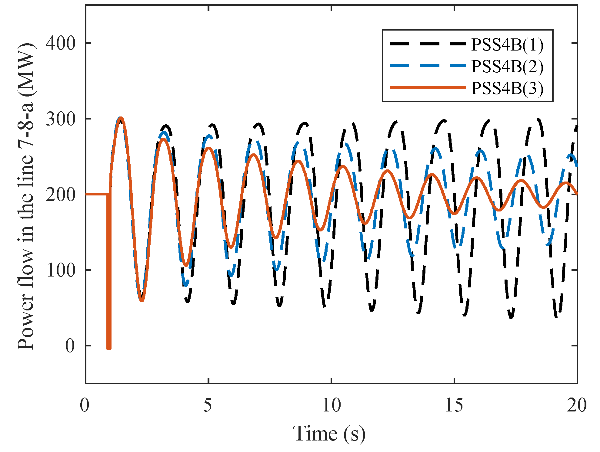
4.1. Results of the Four-Machine/Two-Area Test System

Figure 7 depicts Kundur’s four-machine/two-area system, the details of which are available in [30].
There are three oscillation modes in the original system: one unstable inter-area mode (0.54 Hz) and two stable local modes in each area (around 1 Hz). Generator G1 is selected to install PSS4B, the parameters of which are tuned by the method proposed in order to achieve the following:
  • Stabilize the unstable inter-area mode;
  • Improve the damping of the local mode;
  • Avoid the exciter instability (around 5.5 Hz).
First, the plant transfer function (21) and desired phase–frequency response given by (13) is calculated. Then the typical parameters recommended in IEEE Standard 421.5 [31] are assigned to the three band-pass filters. Subsequently, the space searching approach is utilized to determine the parameters for the phase compensation blocks. The resulting stabilizer is designated as PSS4B(1). Figure 8 illustrates the corresponding CCBode plot with a damping ratio ζ = 0. The magnitude plot reveals two performance peaks: peak 1, which corresponds to the inter-area mode, and peak 2, which corresponds to the exciter mode. By increasing the controller gain while maintaining a fixed phase–frequency response so that the magnitude plot aligns with either peak, an eigenvalue at the corresponding frequency is positioned on the imaginary axis.
After the installation of the PSS4B(1), both the local mode and the inter-area mode move to the left, yet the inter-area mode is still unstable. The magnitude plot suggests that, to shift the inter-area mode across the imaginary axis, we should raise the controller gain so that its magnitude response curve pass through peak 1 at 0.5 Hz. Since the system has no unstable eigenvalue around 5.5 Hz, the performance index Γ(ω) around 5.5 Hz should not be raised to +∞, which means the controller gain around 5.5 Hz should be limited. This is a loop shaping situation, typical in the control community, but not quite usual PSS practice.
To raise the low-frequency gain of the controller while limiting its high-frequency gain, we reset the parameters of the three band-pass filters, and use the space searching approach to tune the phase compensation blocks. Figure 9 shows the CCBode plot of the new PSS4B (designated as PSS4B(2)). It indicates that peak 1 is now beneath the controller magnitude curve while peak 2 is still on top of it. Hence, the new PSS4B is able to stabilize the inter-area mode, which is further confirmed by the eigenvalue calculation result.
To see the results of D-stability, we constructed the CCBode plot with ζ = 3%. By doubling the gain of each branch of PSS4B(2), we can obtain PSS4B(3). Figure 10 and Figure 11 show the corresponding CCBode plots of PSS4B(2) and PSS4B(3), indicating that PSS4B(3) warrants D-stability as well.
Figure 12 shows the simulation results of the test system with different PSS4Bs installed after a three-phase short-circuit on line 7-8-b (cleared after 0.1 s). Table 1 shows the eigenvalues of interest with different PSSs installed at G1. Table 2 lists the parameters of the PSSs.
It can be seen from Figure 12 and Table 1 that PSS4B(2) and PSS4B(3) with the optimized parameters of the three band-pass filters perform better than PSS4B(1), which uses the typical filter parameters. Specifically, the PSS4B(3), with greater gains in each frequency branch, provides more damping for both inter-area mode and local mode, and the increase in gain does not cause the instability of the exciter mode, which verifies the efficiency of the proposed method.

4.2. Results of the North China Power Grid

In recent years, the North China Power Grid has experienced decreased damping ratios, posing a significant limitation for inter-area power transmission. Details of the system analyzed in this study can be found in [4]. This system is characterized by a dominant inter-area mode (between Inner Mongolia and Shandong) at 0.35 Hz. Despite the existing installation of numerous PSS2B stabilizers, the damping ratio of this mode remains below 3%.
For this study, a thermal power plant (Mengxilai 250 MVA) with high participation in the inter-area mode was selected. The desired frequency response was derived from field measurements. Following the methodology outlined in Section 4.1, two stabilizers were designed: PSS4B(4), with typical filter parameters, and PSS4B(5), with optimized filter parameters. Figure 13 and Figure 14 present the CCBode plots (with ζ = 3%) for both PSS4Bs, demonstrating that the installation of PSS4B(5) achieves an inter-area mode damping ratio of no less than 3%. Comparatively, the PSS2B currently in operation at Mengxilai, with a gain Ks1 = 3, would require a gain ten times larger to match the performance of PSS4B(5) in the inter-area mode, which could cause exciter mode instability.
The following conclusions can be drawn from Table 3. First, the currently used PSS2B is very effective in suppressing local oscillation modes, but it cannot provide sufficient damping for inter-area modes. However, due to its higher degree of freedom, PSS4B can provide damping for both local and inter-area modes. Specifically, PSS4B(5) with optimized filter parameters is better than PSS4B(4) with typical filter parameters in suppressing both modes of oscillation without causing exciter mode instability in the system. Table 4 lists the parameters of the PSSs.

5. Conclusions

This paper introduces an iterative design methodology for tuning the parameters of the multi-band power system stabilizer PSS4B using the contoured controller Bode (CCBode) plot. This method combines the benefits of traditional Nyquist and Bode plots, offering vivid and accessible stability margins for the system. Based on the damping index required by the engineering, the corresponding stability margins at the oscillation frequencies of the local mode and the inter-area mode can be obtained. By maximizing the stability margin, the method can flexibly adjust the parameters of the phase compensation block and the band-pass filter to provide greater damping for the corresponding weakly damped modes. The proposed method ensures sufficient damping in the full frequency band of low-frequency oscillations and has good engineering application prospects. It is a valuable enhancement to PSS4B parameter setting techniques in engineering applications. The practicality and effectiveness of the proposed method are demonstrated through case studies involving a four-machine/two-area system and the North China Power Grid.

Author Contributions

Methodology, H.X. and C.J.; Writing—original draft, H.X. and C.J.; Writing—review & editing, H.X. and D.G.; Supervision, C.J. All authors have read and agreed to the published version of the manuscript.

Funding

This research received no external funding.

Data Availability Statement

The original contributions presented in the study are included in the article, further inquiries can be directed to the corresponding author.

Conflicts of Interest

Author Chongxi Jiang was employed by the company Hangzhou Power Supply Company, State Grid Zhejiang Electric Power Co., Ltd. The remaining authors declare that the research was conducted in the absence of any commercial or financial relationships that could be construed as a potential conflict of interest. The authors declare no conflicts of interest.

References

  1. Kundur, P. Power System Stability and Control; McGraw-Hill: New York, NY, USA, 1994. [Google Scholar]
  2. Wang, H.; Du, W. Analysis and Damping Control of Power System Low-Frequency Oscillations; Springer: New York, NY, USA, 2016. [Google Scholar]
  3. Wang, G.; Xin, H.; Gan, D.; Li, N. A probability-one homotopy method for stabilizer parameter tuning. IEEE Trans. Power Syst. 2013, 28, 4624–4633. [Google Scholar] [CrossRef]
  4. Zhou, J.; Shi, P.; Gan, D.; Xu, Y.; Xin, H.; Jiang, C.; Xie, H.; Wu, T. Large-Scale Power System Robust Stability Analysis Based on Value Set Approach. IEEE Trans. Power Syst. 2017, 32, 4012–4023. [Google Scholar] [CrossRef]
  5. Grondin, R.; Kamwa, I.; Trudel, G.; Taborda, J.; Lenstroem, R.; Gerin-Lajoie, L.; Gingras, J.P.; Racine, M.; Baumberger, H. The multi-band PSS: A flexible technology designed to meet opening markets. In Cigré General Session 2000; CIGRE: Paris, France, 2000; pp. 39–201. [Google Scholar]
  6. Grondin, R.; Kamwa, I.; Trudel, G.; Gerin-Lajoie, L.; Taborda, J. Modeling and closed-loop validation of a new PSS concept, the multi-band PSS. In Proceedings of the 2003 IEEE Power Engineering Society General Meeting (IEEE Cat. No.03CH37491), Toronto, ON, Canada, 13–17 July 2003; pp. 1804–1809. [Google Scholar]
  7. Kamwa, I.; Grondin, R.; Trudel, G. IEEE PSS2B versus PSS4B: The limits of performance of modern power system stabilizers. IEEE Trans. Power Syst. 2005, 20, 903–915. [Google Scholar] [CrossRef]
  8. Jia, L.; Gao, X.; Xu, Y.; Xie, H.; Wu, T.; Su, W.; Zhou, J.; Gan, D.; Xin, H. Application of PSS4B stabilizers in suppressing low frequency oscillations: A case study. In Proceedings of the 2015 IEEE Power & Energy Society General Meeting, Denver, CO, USA, 26–30 July 2015; pp. 1–5. [Google Scholar]
  9. Blondel, V.; Gevers, M.; Lindquist, A. Survey on the state of systems and control. Eur. J. Control 1995, 1, 5–23. [Google Scholar] [CrossRef]
  10. Hilhorst, G.; Pipeleers, G.; Michiels, W.; Swevers, J. Sufficient LMI conditions for reduced-order multi-objective H2/H∞ control of LTI systems. Eur. J. Control 2015, 23, 17–25. [Google Scholar] [CrossRef]
  11. Pagola, F.L.; Perez-Arriaga, I.J.; Verghese, G.C. On sensitivities, residues and participations: Applications to oscillatory stability analysis and control. IEEE Trans. Power Syst. 1989, 4, 278–285. [Google Scholar] [CrossRef] [PubMed]
  12. Rouco, L.F.; Pagola, F.L. An eigenvalue sensitivity approach to location and controller design of controllable series capacitors for damping power system oscillations. IEEE Trans. Power Syst. 1997, 12, 1660–1666. [Google Scholar] [CrossRef] [PubMed]
  13. Rouco, L.; Pagola, F.L. Eigenvalue sensitivities for design of power system damping controllers. In Proceedings of the 40th IEEE Conference on Decision and Control (Cat. No.01CH37228), Orlando, FL, USA, 4–7 December 2001; pp. 3051–3055. [Google Scholar]
  14. Rimorov, D.; Kamwa, I.; Joós, G. Model-based tuning approach for multi-band power system stabilisers PSS4B using an improved modal performance index. IET Gener. Transm. Distrib. 2015, 9, 2135–2143. [Google Scholar] [CrossRef]
  15. Wang, Z.; Chung, C.Y.; Wong, K.P.; Tse, C.T. Robust power system stabiliser design under multi-operating conditions using differential evolution. IET Gener. Transm. Distrib. 2008, 2, 690–700. [Google Scholar] [CrossRef]
  16. Kundur, P.; Lee, D.C.; El-Din, H.Z. Power system stabilizers for thermal units: Analytical techniques and on-site validation. IEEE Trans. Power Appar. Syst. 1981, 1, 81–95. [Google Scholar] [CrossRef]
  17. Kundur, P.; Klein, M.; Rogers, G.J.; Zywno, M.S. Application of power system stabilizers for enhancement of overall system stability. IEEE Trans. Power Syst. 1989, 4, 614–626. [Google Scholar] [CrossRef]
  18. Gibbard, M.J.; Vowles, D.J. Reconciliation of methods of compensation for PSSs in multimachine systems. IEEE Trans. Power Syst. 2004, 19, 463–472. [Google Scholar] [CrossRef]
  19. Rogers, G. Power System Oscillations; Kluwer: Norwell, MA, USA, 2000. [Google Scholar]
  20. Kundur, P.; Berube, G.R.; Hajagos, L.M.; Beaulieu, R. Practical utility experience with and effective use of power system stabilizers. In Proceedings of the 2003 IEEE Power Engineering Society General Meeting (IEEE Cat. No.03CH37491), Toronto, ON, Canada, 13–17 July 2003; Volume 3, pp. 1777–1785. [Google Scholar]
  21. Larsen, E.V.; Swann, D.A. Applying power system stabilizers Part III: Practical considerations. IEEE Trans. Power Appar. Syst. 1981, 6, 3034–3046. [Google Scholar] [CrossRef]
  22. Khadraoui, S.; Nounou, H.N.; Nounou, M.N.; Datta, A.; Bhattacharyya, S.P. A measurement-based approach for designing reduced-order controllers with guaranteed bounded error. Int. J. Control 2013, 86, 1586–1596. [Google Scholar] [CrossRef]
  23. Xin, H.; Gan, D.; Huang, Z.; Zhuang, K.; Cao, L. Applications of stability-constrained optimal power flow in the East China system. IEEE Trans. Power Syst. 2010, 25, 1423–1433. [Google Scholar]
  24. Moiseev, S. Universal derivative-free optimization method with quadratic convergence. arXiv 2011, arXiv:1102.1347. [Google Scholar]
  25. Taylor, J.D.; Messner, W. Controller design for nonlinear systems using the Contoured Robust Controller Bode plot. Int. J. Robust Nonlinear Control 2014, 24, 3196–3213. [Google Scholar] [CrossRef]
  26. Taylor, J.D.; Messner, W. Controller Design for Nonlinear Multi-Input/Multi-Output Systems Using the Contoured Robust Controller Bode Plot. In Proceedings of the ASME 2013 Dynamic Systems and Control Conference, Palo Alto, CA, USA, 21–23 October 2013. [Google Scholar]
  27. Ke, D.P.; Chung, C.Y. An inter-area mode oriented pole-shifting method with coordination of control efforts for robust tuning of power oscillation damping controllers. IEEE Trans. Power Syst. 2012, 27, 1422–1432. [Google Scholar] [CrossRef]
  28. Martins, N. Efficient eigenvalue and frequency response methods applied to power system small-signal stability studies. IEEE Trans. Power Syst. 1986, 1, 217–224. [Google Scholar] [CrossRef]
  29. Nakhmani, A.; Lichtsinder, M.; Zeheb, E. Generalized Bode envelopes and generalized Nyquist theorem for analysis of uncertain systems. Int. J. Robust Nonlinear Control 2011, 21, 752–767. [Google Scholar] [CrossRef]
  30. Kamwa, I.; Performance of Three PSS for Interarea Oscillations. Sym-PowerSystems Toolbox. Available online: https://www.mathworks.com/examples/simpower/ (accessed on 1 April 2024).
  31. IEEE Std 421.5-2016 (Revision of IEEE Std 421.5-2005); IEEE Recommended Practice for Excitation System Models for Power System Stability Studies. IEEE: Piscataway, NJ, USA, 2016; pp. 1–207.
Figure 1. Standard IEEE model of PSS4B.
Energies 17 03243 g001
Figure 2. Revised model of PSS4B.
Energies 17 03243 g002
Figure 3. Controller C(s, d) matches a reference model Cr(s).
Energies 17 03243 g003
Figure 4. Block diagram representing installing a PSS to the k-th generator of a multi-machine system.
Energies 17 03243 g004
Figure 5. The Nyquist contour for: (a) Hurwitz stability; (b) D-stability.
Energies 17 03243 g005
Figure 6. Iterative design process of PSS4B.
Energies 17 03243 g006
Figure 7. Four-machine/two-area system.
Energies 17 03243 g007
Figure 8. CCBode plots with ζ = 0: PSS4B(1).
Energies 17 03243 g008
Figure 9. CCBode plots with ζ = 0: PSS4B(2).
Energies 17 03243 g009
Figure 10. CCBode plots with ζ = 3%: PSS4B(2).
Energies 17 03243 g010
Figure 11. CCBode plots with ζ = 3%: PSS4B(3).
Energies 17 03243 g011
Figure 12. Simulation results of four-machine/two-area system.
Energies 17 03243 g012
Figure 13. CCBode plots with ζ = 3%: PSS4B(4).
Energies 17 03243 g013
Figure 14. CCBode plots with ζ = 3%: PSS4B(5).
Energies 17 03243 g014
Table 1. Changes in damping ratios in the four-machine/two-area system with and without PSS.
Oscillation ModeEigenvalueFrequency (Hz)Damping Ratio (%)
NoneInter-area0.055 ± j3.390.54−1.62%
Local−0.591 ± j6.681.068.81%
PSS4B(1)Inter-area0.020 ± j3.420.55−0.59%
Local−0.912 ± j6.561.0413.8%
PSS4B(2)Inter-area−0.028 ± j3.440.550.83%
Local−1.224 ± j6.931.1017.4%
PSS4B(3)Inter-area−0.104 ± j3.470.553.00%
Local−1.956 ± j7.131.1426.4%
Table 2. Parameters of the PSS4B installed at G1.
G1-PSSLow-Frequency BandIntermediate-Frequency BandHigh-Frequency Band
PSS4B(1)KL7.5KI30KH120
FL0.07FI0.7FH8
TL30.0531TI30.3876TH30.1652
TL40.2447TI40.4723TH40.0555
TL50.0531TI50.3876TH50.1652
TL60.2447TI60.4723TH60.0555
PSS4B(2)KL30KI30KH10
FL0.07FI0.7FH8
TL30.3489TI30.2212TH30.4836
TL40.0902TI40.0017TH40.0362
TL50.3489TI50.2212TH50.4836
TL60.0902TI60.0017TH60.0362
PSS4B(3)KL60KI60KH20
Other parameters are the same as for PSS4B(2)
Table 3. Changes in damping ratios in the North China Power Grid with and without PSS.
Oscillation ModeEigenvalueFrequency (Hz)Damping Ratio (%)
NoneInter-area 1−0.053 ± j2.180.352.44%
Local 2−0.950 ± j9.921.589.53%
PSS2BInter-area−0.055 ± j2.180.352.52%
Local−2.626 ± j10.031.6025.31%
PSS4B(4)Inter-area−0.063 ± j2.180.352.92%
Local−5.962 ± j10.031.6050.87%
PSS4B(5)Inter-area−0.068 ± j2.180.353.13%
Local−8.049 ± j10.051.6062.51%
1 Inter-area: Inner Mongolia vs. Shandong. 2 Local: Inner Mongolia.
Table 4. Parameters of the PSS4B installed at Mengxilai.
Mengxilai PSSLow-Frequency BandIntermediate-Frequency BandHigh-Frequency Band
PSS4B(4)KL12.6KI21.7KH47.6
FL0.116FI0.506FH12.1
TL30.3047TI30.3984TH30.4125
TL40.4620TI40.1812TH40.0965
TL50.3047TI50.3984TH50.4125
TL60.4620TI60.1812TH60.0965
PSS4B(5)KL18KI31KH68
Other parameters are the same as PSS4B(4)
Disclaimer/Publisher’s Note: The statements, opinions and data contained in all publications are solely those of the individual author(s) and contributor(s) and not of MDPI and/or the editor(s). MDPI and/or the editor(s) disclaim responsibility for any injury to people or property resulting from any ideas, methods, instructions or products referred to in the content.

