Designing a Dispatch Engine for Hybrid Renewable Power Stations Using a Mixed-Integer Linear Programming Technique

Abstract

Hybrid power plants have recently emerged as reliable and flexible electricity generation stations by combining multiple renewable energy sources, energy storage systems (ESS), and fossil-based output. However, the effective operation of the hybrid power plants to ensure continuous energy dispatch under challenging conditions is a complex task. This paper proposes a dispatch engine (DE) based on mixed-integer linear programming (MILP) for the planning and management of hybrid power plants. To maintain the committed electricity output, the dispatch engine will provide schedules for operation over extended time periods as well as monitor and reschedule the operation in real time. Through precise prediction of the load and the photovoltaic (PV) and wind power outputs, the proposed approach guarantees optimum scheduling. The precise predictions of the load, PV, and wind power levels are achieved by employing a predictor of the Feed-Forward Neural Network (FFNN) type. With such a dispatch engine, the operational costs of the hybrid power plants and the use of diesel generators (DGs) are both minimized. A case study is carried out to assess the feasibility of the proposed dispatch engine. Real-time measurement data pertaining to load and the wind and PV power outputs are obtained from different locations in the Sultanate of Oman. The real-time data are utilized to predict the future levels of power output from PV and from the wind farm over the course of 24 h. The predicted power levels are then used in combination with a PV–Wind–DG–ESS–Grid hybrid plant to evaluate the performance of the proposed dispatch engine. The proposed approach is implemented and simulated using MATLAB. The results of the simulation reveal the proposed FFNN’s powerful forecasting abilities. In addition, the results demonstrate that adopting the proposed DE can minimize the use of DG units and reduce a plant’s running expenses.

1. Introduction

The use of renewable energy (RE) sources has increased recently, given efforts to reduce the need for fossil fuels and minimize the carbon footprint of electrical power systems [1]. By its very nature, renewable energy is a sustainable resource that may, over time, reduce the cost of energy generation and increase energy security. The cost of RE generation has decreased as a result of recent advances in RE technology, and the integration of RE sources into current power systems has increased significantly [1].

Two accessible renewable energy sources that can be used to produce clean electricity are solar and wind power. Recent technological developments have made it possible to harvest power from solar and wind energy installations more cheaply and efficiently [1]. The validity of these sources is a significant question, though. Because wind speed varies, it is impossible to harness all of it. Similarly, solar irradiation varies during the day (and no electricity is produced at night), contributing to the unpredictable nature of solar irradiation [2]. The main difficulties for system operators are variability and ramp events in output power, reserve management, scheduling, and the commitment of generating units. As a consequence, wind and solar sources are non-dispatchable. The challenges brought on by the intermittent nature of these sources must be removed in order to integrate RE sources into the main power system. To provide acceptable electric dependability and power quality, substantial storage systems and traditional backup production must be included, due to the non-dispatchable and intermittent nature of RE sources [3]. The electricity produced by wind and solar power plants may be combined, and a dispatchable power producing station constructed, with the use of correctly sized energy storage systems (ESS). By storing the surplus produced power in the ESS and discharging the ESS when the production of RE sources decreases, a hybrid power plant with ESS, and made up of numerous RE sources, may offer a reliable power supply. The described electrical system is referred to as a hybrid renewable energy system (HRES), a system which combines one renewable energy source with a number of other energy sources. These sources may be conventional, sustainable, or a combination of both, and the system may be utilized independently or as part of a grid [4]. The rising level of system complexity necessitates a cost-effective microgrid design and the development of intelligent management systems that can integrate the operation of various energy sources [5]. With a suitable energy management system and well-designed control structure, a hybrid wind–PV–ESS power plant may remove the fluctuations of the wind–PV power and so constitute a dispatchable RE source, improving system dependability, lowering supply intermittency, and enhancing system security.

To ensure a consistent electricity supply at the point of common coupling (PCC) for power utilities, the generating station must produce stable outputs. There are severe consequences that the electricity producing firm must bear for any departure from earlier commitments. Hence, there is a need to install an emergency power source in case of a failure to provide electricity owing to lower output from PV and wind generators, in order to prevent any expensive penalties. During such crises, electricity can be provided by a diesel- or gas-powered generator. As a result, a dependable hybrid power plant has to have RE generation (wind and/or PV), an ESS, and a diesel or gas backup emergency power supply.

Numerous studies involving distant off-grid regions have shown that several hybrid energy system types are cost-effective generator combinations, including PV/Wind, PV/Diesel, Wind/Diesel, and PV/Wind/Diesel, with or without a storage device [6]. This was demonstrated in [7], which examined the techno-economic viability of a hybridized PV/Wind/Diesel/Batt system for a large non-residential power application. The authors of [7] stated that a carbon-price policy and lower lending rate may support a sizable renewable energy-based project. An ideal hybridized system according to technological, economic, and environmental variables was presented in [8]. The study in [9] looked at the viability of a PV/Wind/Batt/Diesel system used to illuminate a rural location. Comparing the hybrid system to the standard power generating system, the study found that the hybrid system was both economically and ecologically viable.

The energy management system in a microgrid is charged with ensuring that the microgrid runs as efficiently as possible in the presence of probabilistic distributed generation units, interruptible loads, programmable distributed generation units, energy storage units, and the ultimate consumers at the system’s core [10]. A smart microgrid is employed in [11], and it is demonstrated that doing so not only boosts energy efficiency but also makes it possible to create a complementary and efficient network that may enhance dependability and power quality. Moreover [12] introduces a microgrid with an energy management center system, the job of which is to maximize the microgrid’s performance in both island and grid-connected modes. Furthermore, research interest in evaluating the dispatch techniques and optimization algorithms of an islanded microgrid has developed. The study in [2] assesses optimal component sizes, power system responses, and various microgrid cost analyses to analyze the design and optimization of an island-based hybrid microgrid to be used for various load-dispatch techniques.

Economic dispatch (ED), a form of energy management, aims to meet load demand while maintaining a minimal operational cost [13]. An effective ED approach may reduce resource usage and costs while also reducing the release of dangerous greenhouse gases [14]. Due to its efficiency, the ED technique in the context of microgrid design has become a popular topic in recent years [15]. Either a dispersed-control approach or a centralized control strategy can be used to address issues with economic dispatch. The requirement for a bidirectional communication link between the centralized controller and each of the generating units under centralized control raises the cost, the risk of cyber-attack, and the complexity of communication. On the other hand, a distributed-control method employs a dispersed controller that only manages a small region, resulting in a simpler control and communication network [16]. A unique distributed-control approach based on the consensus method has been devised in [17,18] for the resolution of ED issues. In [18], the implemented technique forces the generators to learn about the imbalance between supply and demand. Each generator receives this estimated mismatch data, and as a result, the quantity of power generated is changed to account for the discrepancy. To account for the unpredictability in the generation of renewable energy, [19] proposes a real-time economic dispatch (RTED) approach, together with a subinterval coordination technique, for conventional power plants. In [20], without taking into account communication networks, researchers demonstrated a two-level decentralized optimization strategy that facilitated power dispatch control approaches for an off-grid microgrid. In [21,22], in order to manage the high renewable penetration, the authors designed a reliable energy distribution system, using the distributed economic dispatch technique, for a microgrid.

There have been many distinct two-layer models presented in the literature [23]. The majority of methods disentangle design and dispatch issues by using the fixed architecture systems’ performance evaluation as a fitness metric to direct the exploration of the design space [24]. Mixed integer linear programming (MILP) is a second-layer control technique that is more sophisticated, and suitable for complex system topologies [25]. Utilizing future anticipated behavior of external elements (such as load and solar radiation) to determine the best solution and save operating costs, the MILP formulation employs powerful mathematical algorithms. The authors of [26] demonstrated that, for a rural ICE–BESS–PV microgrid, formal set points optimization can result in significant savings, when compared to simpler heuristic solutions. The two-layer models have the disadvantage that they make it more difficult to include seasonal and annual constraints. Additionally, an iterative process is necessary for an accurate accounting of wearing costs for components whose lifetime is modified by their yearly shipment [27]. The work in [27] presents an improved MILP-based predictive design and dispatch technique. The new approach is contrasted to an earlier heuristic methodology, using local microgrids’ designs and annual performance estimation as examples [27]. One way to formulate a complicated issue that may be solved with MILP is to combine, in a single-layer model, the optimization of design and dispatch. For the optimization of geographically dispersed off-grid microgrids using solar panels and wind turbine generators, a more straightforward model is described in [28]. The model maximizes the quantity, location, and electrical connections between consumption sites, but it ignores the setup and administration of dispatchable generators. In [29], MILP is used to optimize the design of a distributed multi-node CHP system with dispatchable and non-dispatchable DERs in both on-grid and off-grid situations.

An off-grid hybrid microgrid includes controllable and non-controllable generating units as well as a storage system; the use of a two-layer predictive management approach is presented in the study described in [30]. The second layer controls real-time operation and applies a response filter to tame variations in genset load while the higher layer deals with unit commitment. Data from an actual rural microgrid in Somalia are used to evaluate the algorithm, which runs minute-by-minute simulations. The results are contrasted with a newly updated heuristic algorithm and the management technique that is currently in use. The two new techniques reduce fuel use by 15% compared to the prior management system [30]

Furthermore, sizing components and developing an efficient operation plan are essential steps in ensuring the competitiveness of off-grid systems in order to reduce the levelized cost of electricity (LCOE) for their consumers. Various strategies can be used, as shown in

Table 1. Strategies for sizing components.

Model Type	Analytical	Two Layers		Single Layer
Design identification (layer 1)	Analytical expression	GA, PSO, Pattern search		MILP
Dispatch strategy (layer 2)	Simulation not performed	Heuristic	LF	MILP
			CC
			ABV
		MILP

[27].

Analytical models that only need assumptions on the total energy consumption and the technological capabilities of the various components can be used to estimate off-grid LCOE [31]. These models have the benefit of requiring extremely small amounts of computing time, and as a result, they are the technique of choice for estimating off-grid costs in early electrification planning studies. However, they do not specifically address the design and dispatch issue, which might result in an inaccurate LCOE calculation. More sophisticated simulation-based design methods which choose the sizes of components based on the predicted performance of potential solutions over a reference period can get around this restriction [27]. A quick and accurate method of replicating the operation of the microgrid is to use heuristic dispatch logics. Because of the state of the art in commercially available hardware, they consist of a set of established rules that regulate the system depending on its condition and the features of the installed equipment. They also have the advantage of being easily deployable in actual systems [27]. They are integrated into the popular HOMER simulation-based microgrid design optimization program [32].

The concept of optimization and the optimization methods utilized for hybrid renewable power plant with several generation sources require the dispatch of electricity from each of the sources in accordance with the requirements stated by the operator or controller. A description of the sizes, energy levels, and power capacities of each system component, the design of which was predetermined, is the primary output of an optimization process in a RES in its most basic form. It is possible to carry out a more complicated level of optimization, such as real-time system reconfiguration by the controller (such as energy routing through electricity, hydrogen, or both), over a variety of potential configurations of the system’s parts. To what extent a system will function and meet its technical and non-technical design objectives depends greatly on the component configuration and the size choices made [33]. Consequently, such a controller may also be referred to as a “Dispatch Engine (DE)” [34]. In order to ensure the necessary power flow through all devices, the DE for a hybrid power plant, which is a real-time control system, must precisely and quickly handle various power sources and an ESS [2].

There are several objectives in a hybrid system that require optimization, including management, control, and sizing. The most popular optimization techniques employed in the past few years are listed in this section. The three categories of optimization techniques include classical techniques, artificial techniques, and hybrid techniques [35,36].

Table 2. Optimization techniques for hybrid renewable energy systems.

Optimization Techniques		Refs.
Classic techniques [36]	Linear programming model (LPM)	[37,38]
	Multi choice goal programming (MCGP)	[39]
	Multi-objective evolutionary algorithms (MOEA)	[40,41]
	Mixed integer linear programming (MILP)	[27,42]
	Dynamic programming (DP)	[43]
	Nonlinear programming (NLP)	[44]
Artificial techniques	Fuzzy logic	[45,46,47,48]
	Genetic algorithm	[49,50,51,52,53]
	Neural network	[54,55]
	Particle swarm optimization (PSO)	[56,57,58]
	Adaptive neuro-fuzzy inference system (ANFIS)	[59,60]
	Fuzzy analytic hierarchy process (AHP)	[61,62,63,64]
	Fuzzy genetical algorithm	[63,64]
	Fuzzy analytic network process	[65]
	Fuzzy TOPSIS	[66,67]
	Fuzzy clustering	[68]
Hybrid techniques		[33,69,70,71,72,73,74]

summarizes these techniques, as used.

While several studies have explored hybrid renewable energy systems, optimization, and power forecasting techniques, none have specifically addressed PV–DG–ESS–Grid hybrid renewable energy systems with precise forecasting using real-time data, particularly in the context of Oman. Therefore, there is a research gap that needs to be addressed. The present paper introduces the DE as a solution to this gap, aiming to fill the aforementioned research void and examine the feasibility of implementing such a strategy in Oman. By incorporating real-time data and considering the unique operational conditions of Oman, the DE seeks to enhance the accuracy and efficiency of forecasting and optimization for PV-DG-ESS-Grid hybrid plants in the region.

The objective of this study is to design a DE for a hybrid power plant of wind power, solar power, diesel engines, and ESS. When a utility requests ancillary services, the proposed dispatch engine would maximize resource use to account for any unusual changes in load circumstances. The DE will involve a combination of algorithms and models to predict the power output of each renewable energy source and optimize the dispatch of power between the different sources to meet the demand, while minimizing costs and maximizing the use of renewable energy. ‘Forecasting’ and ‘Real-time operator’ are the two steps that make up the proposed DE. A long-term plan for the plant’s operations throughout the subsequent time period is what the first stage is meant to provide. The hybrid power plant can utilize this strategy to commit on an hourly basis to taking part in utility load-sharing and the energy markets. The second stage will monitor plant operations and rearrange them in accordance with the current condition of the hybrid plant’s parts.

With the use of the real load, PV, and wind data from a region in the Sultanate of Oman, the suggested dispatch engine’s feasibility has been evaluated. Oman’s ambition in increasing electricity production is to lessen its reliance on natural gas as a fuel source and support the new government fuel-diversification program [75]. As stated in the Oman 2040 Vision, the development of unconventional sources employing natural resources, including RE sources, would help lower production costs and improve a variety of economic sectors’ competitiveness. The strategy aims to attain 20% renewable energy consumption relative to overall consumption by 2030, and 35% to 39% by 2040 [76]. Therefore, implementing such a DE in Oman will be a great step toward the success of this plan.

The rest of the paper is structured as follows: Section 2 provides mathematical representations of the hybrid power system’s component parts. The proposed DE is presented in Section 3. The model of the suggested system is developed in Section 4, and the MILP approach is then introduced in Section 5. The forecasting method is described in Section 6. Section 7 presents the case simulation, while Section 8 presents the associated simulation findings. Finally, Section 9 provides the conclusions.

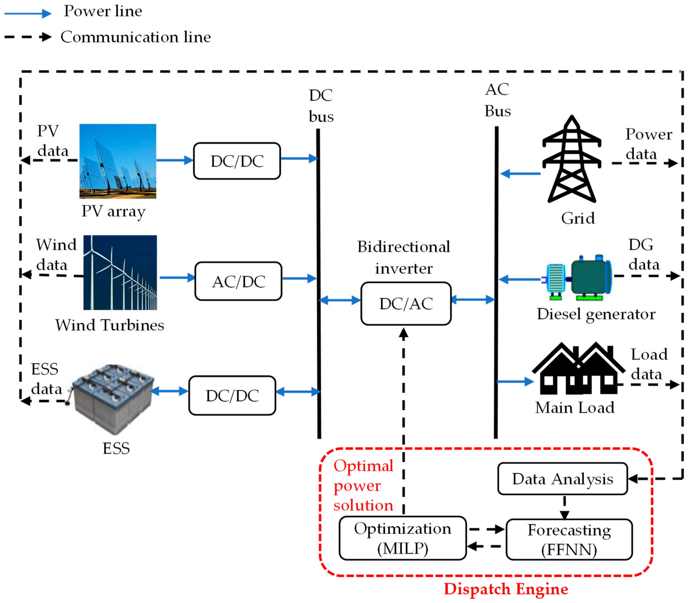
2. Proposed Hybrid System

Figure 1 depicts the functional block diagram of the proposed DE. The proposed approach considers a microgrid consisting of a diesel generator (DG), a wind energy conversion system, a PV system, and an ESS system. The interconnection to a main grid and load for energy transfer is performed through a bidirectional inverter. Generally, RES, ESS, and grid are interconnected via a DC bus facilitated by converters. This configuration allows for the ESS to be charged from the grid or the RES. Moreover, the ESS has the capability to release power to either the grid or loads.

2.1. The ESS Model

Equations (1)–(5) may be used to compute the ESS’s operation and state of charge (SoC), subject to the limitations imposed by Equations (6)–(9), as shown below.

Discharge is computed by the following equation:

$$E_{\mathit{ESS}}(t)=E_{\mathit{ESS}}(t-1)+P_{\mathit{ESS}}(t)\raisebox{1ex}{$∆t$}\!\left/ \!\raisebox{-1ex}{${\eta }_{\mathit{dis}}$}\right.,P_{\mathit{ESS}}(t)=-\mathit{ve}$$

(1)

Charge is computed by the following equation:

$$E_{\mathit{ESS}}(t)=E_{\mathit{Ess}}(t-1)+P_{\mathit{ESS}}(t)∆t{\eta }_{\mathit{ch}} , P_{\mathit{ESS}}(t)=+\mathit{ve}$$

(2)

$$\mathit{SoC}=\frac{E_{\mathit{ESS}}(t)}{E_{\mathit{ESS}}^{\mathit{max}}}$$

(3)

Power limits are computed by the following equation:

$$P_{ESS}^{dis}\le \frac{P_{ESS}(t)}{{\eta }_{dis}}\le 0, P_{ESS}(t)=-ve$$

(4)

$$0\le P_{ESS}(t){\eta }_{ch}\le P_{ESS}^{ch}, P_{ESS}(t)=+ve$$

(5)

Storage energy limits are computed by the following equation:

$$0\le E_{ESS}(t)\le E_{ESS}^{max}$$

(6)

State of charge limits are computed by the following equation:

$${SoC}^{min}\le SoC(t)\le {SoC}^{max}$$

(7)

Starting operation of energy is computed by the following equation:

$$E^{int}=\frac{{SoC}^{min}}{E_{ESS}^{max}}$$

(8)

Starting and ending of the state of charge are computed by the following equation:

$${SoC}^{int}={SoC}^{end}$$

(9)

For all of the above equations, $P_{ESS}$ is the ESS’s power output (MW), $E_{ESS}$ is its stored energy (MWh), and ∆t is the interval’s time, which is equivalent to one hour. The discharge and charge efficiencies are denoted by ${\eta }_{dis}$ and ${\eta }_{ch}$, respectively. The ESS’s state of charge is represented by SoC, its maximum energy storage (MWh) by $E_{ESS}^{max}$, and its maximum charging and discharging powers (MW) by $P_{ESS}^{ch}$ and $P_{ESS}^{dis}$, respectively. The state of charge’s maximum and lower bounds are denoted by ${SoC}^{max}$ and ${SoC}^{min}$, respectively. Positive and negative values are denoted by $ve$ and $-ve$, respectively. $E^{int}$ is the energy stored in the ESS at first (MWh), and ${SoC}^{int}$ is the ESS’s charge level at the end of the previous day. At the start of the day, ${SoC}^{end}$ is the ESS’s state of charge [77].

2.2. PV Array Modeling

The proper connections of the PV cells determine the output of the PV panels. PV cells are linked in series to create a string, in order to provide the necessary output voltage in the PV panel. Conversely, comparable strings are linked in parallel to boost a panel’s output-current capacity. This creates a PV panel or PV module, the output power rating of which is calculated by multiplying the output side’s voltage and current [78]. A number of models were created in [79] to calculate the PV panel output power, or $P_{pv-out}$. However, a straightforward model that accounts for two variables—ambient temperature and solar irradiance—has been employed in this investigation. This model’s output power may be acquired as follows [80]:

$$P_{pv-out}(t)=P_{N-pv}\times \frac{G_t(t)}{G_{t-STC}}\times \left[1+{\alpha }_t\left(T_C(t)-T_{C-STC}\right)\right]$$

(10)

where $P_{pv-out}$ is the PV module’s output power (W); $P_{N-pv}$ is its rated power (W) at standard test condition (STC), usually, specified by the manufacturer; $G_t$ is the solar irradiance (W/m²); $G_{t-STC}$ is the solar irradiance at STC ($G_{t-STC}$ = 1000 W/m²); ${\alpha }_t$ is the temperature coefficient; $T_{C-STC}$ is the cell temperature at STC (T_C-STC = 25 °C); and $T_C$ is the cell temperature (°C) [80].

2.3. Wind Turbine Modeling

The wind turbine generator’s output power fluctuates in tandem with variations in wind speed, which is dependent on altitude for the same spot. As a result, the wind speed reported at the anemometer height needs to be corrected to the wind turbine’s hub height [81]. In this case, the wind speed vertical profile of a given site is determined using two mathematical models, such as the log-law and the power law. The power-law model is used in this study to determine the wind profile, as shown below [80].

$$V_2=V_1·{\left(\frac{h_2}{h_1}\right)}^{\alpha }$$

(11)

where $V_1(\mathrm{m}/\mathrm{s})$ describes the wind speeds at the anemometer and $V_2(\mathrm{m}/\mathrm{s})$ describes the wind speeds at hub height ($h_1(\mathrm{m})$ and $h_2(\mathrm{m})$), and $\alpha$ is the power-law exponent. $\alpha$ is dependent on a number of variables, including temperature, wind speed, terrain roughness, height above ground, daytime hours, and season [80].

Based on the following equation, the wind turbine generator’s output power may be assessed [80,82].

$$P_{wt}(t)=\left\{\begin{array}{cc}0\hfill & V\le V_{cut-in} or V\ge V_{cut-out}\\ P_r·\frac{V^3-V_{cut-in}^3}{V_r^3-V_{cut-in}^3}\hfill & V_{cut-in}<V<V_{rated}\\ P_r\hfill & V_{rated}<V<V_{cut-out}\end{array}\right.$$

(12)

where $V$ is the wind speed (m/s); $P_r$ is the rated power (kW); and $V_{cut-in}$, $V_{rated}$, and $V_{cut-out}$ stand for the WT’s cut-in, rated, and cut-out wind speeds, respectively, in m/s. The manufacturer often specifies these settings.

A wind turbine generator’s rated power $P_r$ (W) may be stated as a function of the air density $p_{air}$, the rated wind speed, the maximum power coefficient $C_p$, and the area swept by the blades.

$$P_r=\frac{1}{2}{C}_p\times p_{air}\times A_{wind}\times V_r^3$$

(13)

2.4. Diesel Generator Modeling

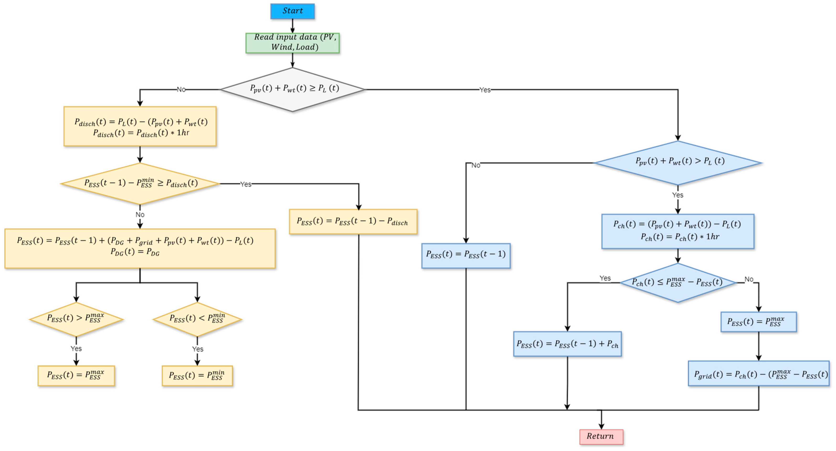
According to studies in the literature, the fuel cost per year that the generator will need to operate during the system’s lifetime is calculated as follows.

$$C_{DG}=C_F\times \sum _{t=1}^{8760}F(t)$$

(14)

where $C_F$ is the unit fuel cost and $F(t)$ is the hourly fuel consumption of the generator, which is evaluated by the following equation:

$$F(t)=A\times P_{DG}(t)+B\times P_R$$

(15)

where $P_{DG}(t)$ is the power generated (KW) at time $t$, $P_R$ is the rated power of the generator, and $A$ and $B$ are the fuel curve coefficients.

In order to guarantee a constant supply of power to the load, the diesel generator is employed as a backup source when the energy from renewable energy sources (wind and PV) and batteries is unable to satisfy the demand; in other words,

$$\frac{P_l(t)}{{\eta }_{inv}}>P_g(t)+\left[SOC(t-1)-(1-DOD)\right]\times 1000\times N_b\times C_b$$

(16)

Therefore, the needed power $P_{DG}\left(t\right)$ from the diesel generator is stated as follows:

$$P_{DG}(t)=P_l(t)-\left\{P_g(t)+\left[SOC(t-1)-(1-DOD)\right]\times 1000\times N_b\times C_b\right\}\times {\eta }_{inv}$$

(17)

If the needed power $P_{DG}(t)$ is more than the generator-rated power of $P_R$, the loss of power supply ($LPS$) is computed by

$$LPS=P_{DG}(t)-P_R$$

(18)

3. Dispatch Engine

By efficiently employing RESs and ESSs, the suggested DE in Figure 1 seeks to enhance hybrid plant profitability. In order to estimate the electricity demand, predict the power output of each renewable energy source, and optimize the dispatch of power between the various sources to meet the demand, while minimizing costs and maximizing the use of renewable energy, the DE for a hybrid renewable power station would typically involve a combination of algorithms and models. Many data sources are accessible during the data analysis phase, including the grid, RES stations, ESS data, and DG data.

The following actions would probably be included in the code for such a system:

• Data collection: Compile information on the historical and present electricity consumption, as well as the power production of each renewable energy source.
• Forecasting: Over the following several hours or days, estimate the power production of each renewable energy source and the amount of electricity that will be consumed using models and algorithms.
• Optimization: Employ algorithms for optimization to determine the best way to distribute electricity among the various sources in order to satisfy the anticipated demand while minimizing expenses and optimizing the usage of renewable energy. This may entail figuring out whether to utilize ESS or grid electricity, as well as the most effective mix of renewable energy sources to employ.
• Control: To maintain system stability and stay within operating parameters, use control algorithms to modify each source’s output power in accordance with the dispatch plan.

Four different EMS will be employed in this study:

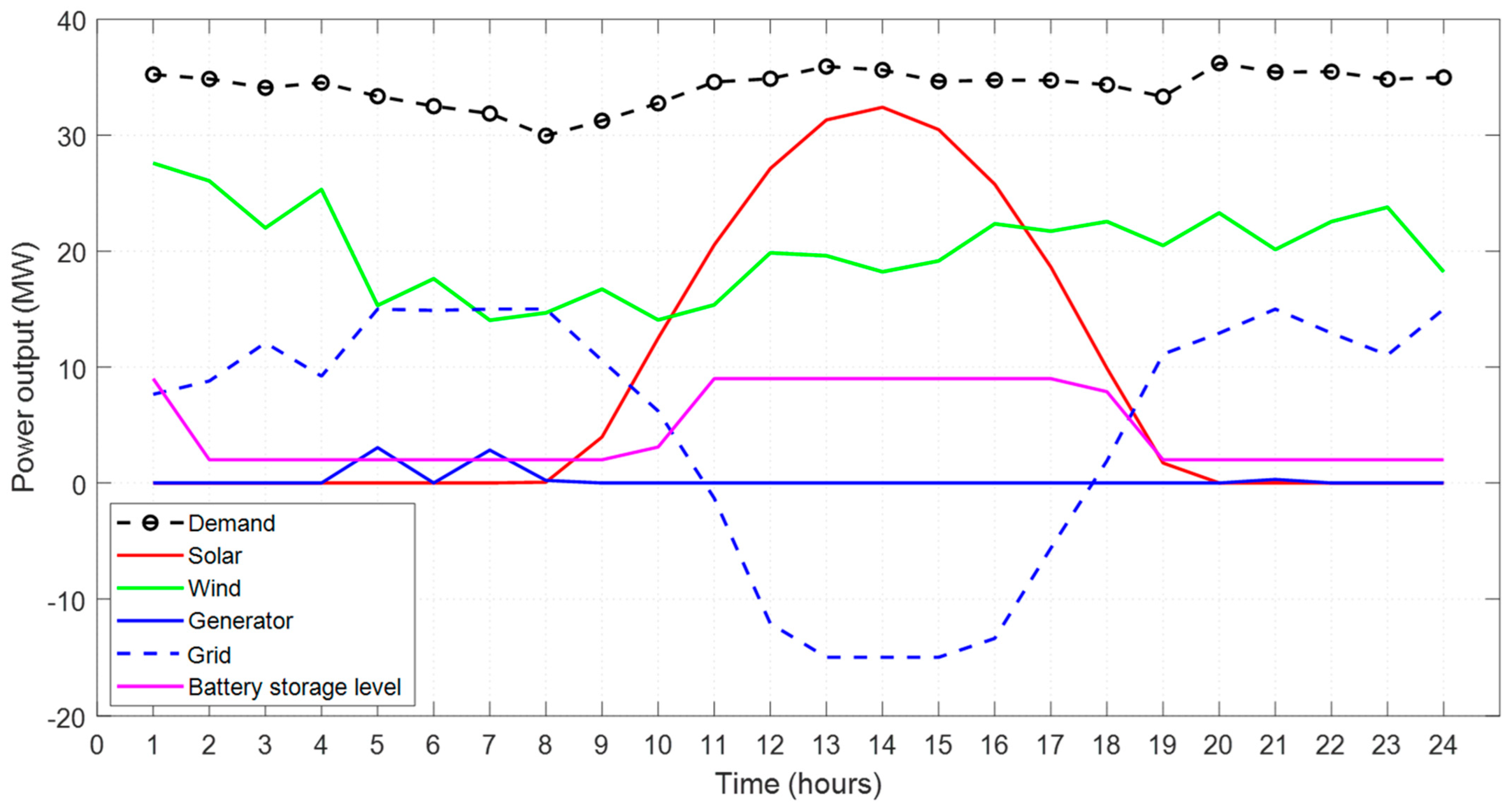
• Mode 1: In this mode, the load-demand need is met by the electricity generated from renewable energy sources (PV and WT). The ESS is charged using the excess energy.
• Mode 2: When the ESS is completely charged, the power provided from renewable energy sources surpasses the load-demand need. Here, the extra energy is sent to the grid.
• Mode 3: In this mode, the amount of electricity produced by renewable sources is insufficient to meet the demands of the load. In this instance, the ESS will make up the difference in power generation to meet the demands of the load.
• Mode 4: In this mode, the ESS level is low, and the electricity provided from renewable energy sources is insufficient to fulfill the load demand. In this situation, the system will draw the needed power from the grid. If the power drawn from the grid reaches its maximum allowed level, the DG will run to make up for the shortfall in power supply to meet the demands of the load and further guarantee the ESS charge.

The suggested EMS algorithm flowchart utilized in the present research is displayed in Figure 2.

4. Problem Formulation

Optimal outcomes are achieved through the identification of parameter settings that minimize a specific function, which in turn offers stakeholders a quantifiable insight into the added value of the system. To locate the function’s minimum value, mathematical programming methods are frequently employed. These techniques navigate through predefined variables, aiming to find the optimal solution while adhering to a defined set of constraints. This process not only aids in optimizing system performance, but also ensures that the solutions are feasible and aligned with the system’s operational limits and goals [83]. The problem can be described as expressed below:

$$\mathrm{Find} \mathrm{X}=\left\{\begin{array}{c}{\mathrm{x}}_1\\ {\mathrm{x}}_1\\ \begin{array}{c}·\\ \begin{array}{c}·\\ {\mathrm{x}}_{\mathrm{n}}\end{array}\end{array}\end{array}\right\}\mathrm{which} \mathrm{minimizes} \mathrm{F}(\mathrm{X})$$

(19)

within constraints

$$\begin{array}{c}{g}_j\left(x\right)\le 0,j=1,2\dots ,m \\ l_j\left(x\right)\le 0,j=1,2\dots ,p\end{array}$$

(20)

where $\mathrm{F}(\mathrm{X})$, $\mathrm{X}$, $g_j\left(x\right),$ and $l_j\left(x\right)$ are the objective function, n-dimensional design vector, and inequality and equality constraints, respectively. Term $n$ is the number of variables, and $m$ and/or $p$ are the numbers of constraints [83].

Various mathematical optimization techniques can be applied based on the problem’s characteristics, especially in the context of renewable energy systems, as will be elaborated in the subsequent sections. The aforementioned DE has the primary goal of minimizing the costs of the hybrid plant and maximizing the use of RESs. To achieve this objective, each component relevant to the preceding statement needs to be precisely defined. Hence, the mathematical expression of the economic cost objective function $C_{Total}$ can be formulated as

$${{\mathit{minC}}_{\mathit{Total}}=C}_{\mathit{wind}}+C_{\mathit{PV}}+C_{\mathit{ESS}}+C_{\mathit{DG}}{+C}_{\mathit{grid}}$$

(21)

where $C_{\mathit{Total}}$ is the total cost function, $C_{\mathit{wind}}$ is the cost function for wind power generation, $C_{\mathit{PV}}$ is the cost function for PV power generation, $C_{\mathit{ESS}}$ is the cost function for the ESS, $C_{\mathit{DG}}$ is the cost function for the DG, and $C_{\mathit{grid}}$ is the grid cost function. All cost functions in the model carry equal weightage, as the primary objective is to minimize the operating costs of the plants. Each cost function contributes to the same overarching goal and is of equal significance.

The cost function for the DG ($C_{\mathit{DG}})$ is formulated as the aggregate of the fuel cost required for generating enough energy to meet grid demands and the associated emission costs. Given that CO₂ accounts for around 99% of total emissions, the model overlooks the minor gases. With the mass of gases emitted from diesel combustion known, the emission cost can be quantified based on the amount of fuel consumed. Hence the cost function of the DG can be expressed as

$$C_{\mathit{DG}}=\sum _{t=1}^{t+N}∆t ·\left(\frac{P_{DG}^G.F}{P_{DG}^{max}}·(C_f+C_m{\alpha }_{c{o}_2})\right) \forall t\in \left[1,T\right]$$

(22)

where $P_{DG}^G$ is the DG-generated power, F is the amount of diesel used per kWh, $P_{DG}^{max}$ is the maximum power produced by DG, $C_f$ the cost of fuel per liter, ${\alpha }_{c{o}_2}$ is the gas mass associated with burning fuel, and $C_m$ is the cost of said gases.

The grid cost function $C_{\mathit{grid}}$ is defined as the difference between the cost of power purchased and the cost of power sold for each time interval.

The performance of the system is governed by a number of constraints on the proposed cost function. The power balance constraint is the first set of constraints; it ensures that at any time t, the total power generated from DG ($P_{\mathit{DG},t})$, wind $(P_{\mathit{wind},t})$, and PV ($P_{\mathit{PV},t})$, as well as the power imported or exported from or to the grid ($P_{\mathit{grid},t})$, and power used for ESS ($P_{\mathit{ESS},t})$, equals the total load power ($P_{L,t})$.

The power balance constraint is established as follows:

$$P_{\mathit{PV},t}+P_{\mathit{wind},t}+P_{\mathit{ESS},t}+P_{\mathit{DG},t}+P_{\mathit{grid},t}=P_{L,t} \forall t\in \left[1,T\right]$$

(23)

where $P_{\mathit{PV},t}$ is the PV power, $P_{\mathit{wind},t}$ is the wind power, $P_{\mathit{ESS},t}$ is ESS power, $P_{\mathit{DG},t}$ is the measured DG power, $P_{\mathit{grid},t}$ is the grid power, $P_{L,t}$ is load power, and $T$ is the operation time.

The second constraint is the generation-limits constraint for the wind generators. The upper and lower limitations of the wind farm’s output power are among the operating constraints [84].

$${0\le P}_{\mathit{wind},t}\le P_{\mathit{wind}}^{\mathit{max}} \forall t\in \left[1,T\right]$$

(24)

where $P_{\mathit{wind}}^{\mathit{max}}$ is the maximum power output of the wind farm.

The third constraint is the generation-limits constraint for the PV generators.

$${0\le P}_{\mathit{PV},t}\le P_{\mathit{PV}}^{\mathit{max}} \forall t\in \left[1,T\right]$$

(25)

where $P_{\mathit{PV}}^{\mathit{max}}$ is the maximum power of the PV power station.

In order to balance the ESS’s SoC throughout the charging and discharging cycles, a fourth constraint is established. The constraints of the ESS include power capacity limits [84]:

$$P_{\mathit{ESS},\mathit{min}}(t)\le P_{\mathit{ESS}}(t)\le P_{\mathit{ESS},\mathit{max}}(t), \forall t\in \left[1,T\right]$$

(26)

where $P_{\mathit{ESS},\mathit{min}}$ and $P_{\mathit{Ess},\mathit{max}}$ are, respectively, the lower and upper limits of the ESS’s power.

To prevent the ESS from being over-charged and over-discharged, its SoC limit is expressed as follows:

$${\mathit{SoC}}_{\mathit{min}}(t)\le {\mathit{SoC}}_{ESS}(t)\le {\mathit{SoC}}_{\mathit{max}}(t), \forall t\in \left[1,T\right]$$

(27)

where ${\mathit{SoC}}_{\mathit{min}}$ and ${\mathit{SoC}}_{\mathit{max}}$ are, respectively, the minimum and maximum bounds of SoC.

Capacity, charge, and discharge power, and charge and discharge state constraints, are some of the constraints placed on the ESS. The following are the precise formulae.

$$\left\{\begin{array}{ll}{E^{\mathit{min}}\le E}_t\le E^{\mathit{max}}& \forall t\in \left[1,T\right]\\ {0\le P}_t^c\le P^{c,\mathit{max}}& \forall t\in \left[1,T\right]\\ {0\le P}_t^d\le P^{d,\mathit{max}}& \forall t\in \left[1,T\right]\\ c_t+d_t\le 1& \forall t\in \left[1,T\right]\\ {P_t=c_{t}P}_t^c+d_t{P}_t^d& \forall t\in \left[1,T\right]\\ \hfill E_t=\frac{E_{t-1}+P_t^c{\eta }^c\Delta t-P_t^d\Delta t}{{\eta }^d}\hfill & \end{array}\right.$$

(28)

where $E_t$, $E_{t-1}$ are the capacities of the ESS at time $t$ and time $t-1$; $E^{\mathit{max}}$, $E^{\mathit{min}}$ are the maximum and the minimum capacities of the ESS; $P_t^c$, $P_t^d$ are the charge and discharge power of the ESS at time t; $P^{c,\mathit{max}}$, $P^{d,\mathit{max}}$ are the maximum charge power and the maximum discharge power of the ESS; $c_t$, $d_t$ are the states of charge and discharge of the ESS at time t; $c_t$ = 0 means a lack of charge of the ESS at time t; $c_t$ = 1 means that the ESS holds a charge at time t; $d_t$ = 0 means a lack of discharge of the ESS at time t; $d_t$ = 1 means that the ESS is discharged at time t; ${\eta }^c$, ${\eta }^d$ are the charge and the discharge efficiencies, respectively; and $\Delta t$ is the unit time interval [85].

The fifth set of constraints is related to DG power and ensures that the generator limits are not exceeded. The upper and lower limitations of the output power are among the DG constraints.

$${0\le P}_{\mathit{DG},t}\le P_{\mathit{DG}}^{\mathit{max}} \forall t\in \left[1,T\right]$$

(29)

where $P_{\mathit{DG}}^{\mathit{max}}$ is the DG unit’s maximum power.

The last set of constraints is related to the maximum amount of power that may be transferred between the main grid and the microgrid. This power is limited between maximum and minimum values to ensure the system’s transmission safety. Constraints include the output power’s upper and lower limits, the minimum power purchased, and the maximum power sold, as defined in Equation (11).

$$P_{\mathit{grid},\mathit{min}}(t)\le P_{\mathit{grid}}(t)\le P_{\mathit{grid},\mathit{max}}(t), \forall t\in \left[1,T\right]$$

(30)

where $P_{\mathit{grid},\mathit{max}}$ and $P_{\mathit{grid},\mathit{min}}$ are the grid’s maximum and minimum power limits.

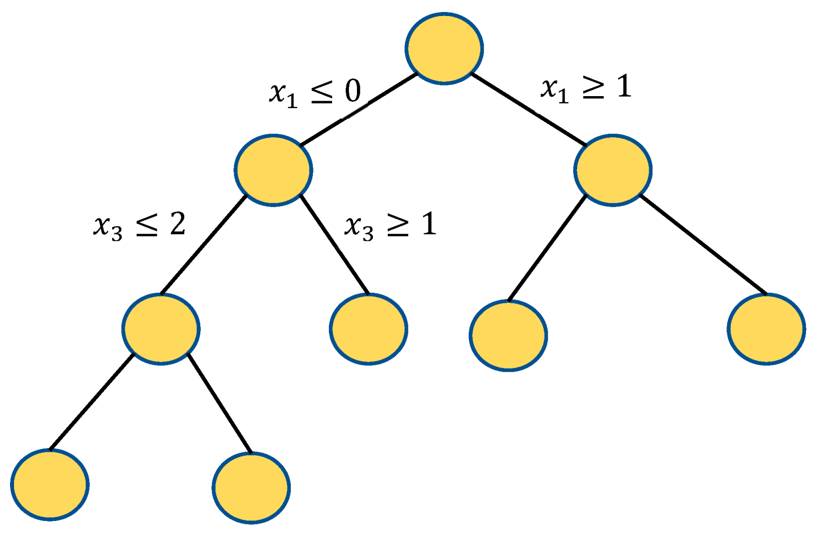
5. Mixed-Integer Linear Programming (MILP)

The MILP approach will be utilized to address the optimization issue presented in the preceding section. As such, this method follows the traditional MILP framework, focusing on minimization. This approach is especially well-suited for optimizing complicated systems with several choice variables because of its ability to handle issues involving both discrete and continuous variables. Subject to a set of linear constraints, the research seeks to identify the most effective solution that minimizes the objective function by utilizing MILP. This method ensures that the solution path is well-structured and also makes it easier to manage the many technical and operational limitations that are present in the optimization issue. Only $c_t$ and $d_t$ in ESS constraints are integers; all other arguments are real variables. Regarding the ESS’s charging/discharging cycles’ either/or behavior, the variables $c_t$ and $d_t$ are considered as binary (integer) variables.

MILP is a powerful mathematical optimization approach that finds the best solution within a feasible set using a well-defined objective function and a set of constraints. MILP stands out from other optimization tactics, such as classical linear programming, intelligent algorithms, and hybrid methods, due to its better precision and computing efficiency. This methodology’s strength is its ability to efficiently include both discrete and continuous variables in the decision-making process, allowing for a thorough examination of complicated systems. The decision to use MILP as the selected optimization method for this study was due to its proven effectiveness in generating highly accurate solutions in a timely way, making it a useful tool for solving complex optimization difficulties [86].

To address MILP issues, three key strategies stand out for their effectiveness and efficiency: the feasibility pump technique, cutting edge methods, and tree search algorithms. The descriptions of those techniques are set forth below:

• The feasibility pump technique aims to quickly identify a viable solution that meets all issue constraints. It alternates between solving a relaxed linear problem to enhance objective value and rounding answers to retain feasibility under integer constraints. The feasibility pump is especially beneficial for quickly creating a viable starting point which may then be refined using other methods.
• Cutting Plane methods: These approaches, which rely on continually refining the viable solution space, apply extra constraints to remove regions that lack the optimal solution. These cuts are made with the solution of the linear relaxation of the MILP problem, which is gradually tightened to converge to the integer solution. This method is beneficial for reducing the search space and shortening the solution time for complex problems.
• Tree Search Algorithms: These algorithms, such as branch-and-bound and branch-and-cut, employ systematic exploration to identify viable solutions. They function by breaking down the solution space into smaller subproblems (branching) and assessing the limits of these subproblems to remove those that do not contain the optimal solution. Tree search algorithms are effective tools for tackling MILP issues because they can handle both the combinatorial character of integer variables and linear correlations between variables effectively.

Each of these techniques has distinct benefits and may be chosen based on the specific characteristics of the MILP issue at hand, such as its size, the nature of the constraints, and the desired balance of solution precision and computational time. Additionally, putting these strategies together or employing them in a planned sequence can considerably improve the efficiency of addressing MILP problems, leading the way in identifying ideal solutions in many applications [87].

The tree search technique, also known as branch-and-bound, is the approach that has been selected to solve the MILP issue. This approach is an algorithmic method crucial for solving MILP problems. Because of its architecture, it is possible to explore the solution space of MILP issues in a systematic way with the goal of precisely and effectively identifying the best or nearly optimal solution [87].

Using the MILP tree search approach, a search tree is constructed, with each node corresponding to a different subproblem inside the larger MILP framework. This procedure begins with the creation of a starting node that contains the full problem. It then branches depending on the variables, which must meet integer constraints, to split the problem down into more manageable sub-problems. Figure 3 depicts an enumeration tree as the fundamental representation of the branch-and-bound method. A linear relaxation of the subproblem is carried out at each node in order to provide a lower bound for the ideal goal value. After branching, the algorithm uses linear programming to solve the relaxed linear version of each subproblem at the child nodes in order to determine an upper bound for the ideal goal value. Bounding is an essential phase in the MILP tree search process which improves the search’s efficiency and focus by fine-tuning the bounds using the output of linear programming relaxations. The search continues, gradually tightening its limits, until all nodes in the search tree have been explored or a predetermined stopping requirement is satisfied. The approach finds the best or nearly best possible integer solution to the initial MILP challenge through this painstaking search procedure, ultimately identifying the most efficient answer within the stated solution space [88].

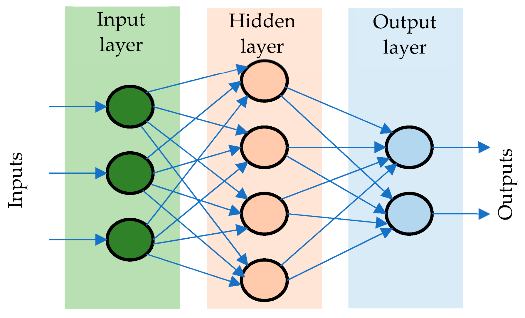
6. Wind, PV, and Load-Power Forecasts

PV and wind energy are unpredictable and intermittent. This will affect the accuracy of the economic dispatch findings if the unpredictable data for wind and PV power are employed to solve the problem. In order to forecast wind and PV power, historical data must be used. Moreover, designing a robust and efficient EM that capitalizes on renewable energy sources necessitates a detailed and precise understanding of the load profile. The variability inherent in load profiles is a critical factor that influences the overall system reliability. Therefore, our research underscores the significance of precise load-power forecasting to ensure the reliability and efficiency of energy management.

For effective PV, wind, and load power forecasting, leveraging historical consumption data is imperative. By analyzing data from previous periods, neural networks can predict information associated with the future. Therefore, to forecast PV, wind, and load power, neural networks are utilized [89,90]. These models are adept at interpreting complex data patterns, enabling them accurately to predict future events based on historical data.

Incorporating neural networks into our forecasting methodology is a cornerstone of our approach. With their ability to learn and adapt, neural networks offer a powerful tool for predicting future PV, wind, and load power with high accuracy. This predictive capability is instrumental in optimizing the operation of renewable energy sources within the EMS, ensuring that energy supply aligns closely with demand patterns. Consequently, neural network-based forecasting represents a pivotal component of our strategy to enhance the efficiency and reliability of energy management in systems reliant on renewable energy sources [89,90].

Feed-Forward Neural Networks

In this study, we provide a feed-forward neural network (FFNN)-based forecasting model. As shown in Figure 4, a neural network’s architecture is made up of nodes, or neurons, arranged in three different levels: the input layer, one or more hidden layers, and the output layer. Weighted parameters are used to construct connections between nodes across these layers by measuring the strength of each link. The topology of the network produced by this arrangement is highly linked and replicates the structure of the biological nervous system. Every node in a layer is intimately connected to every other layer’s node, creating a complete network that makes intricate data processing and pattern recognition jobs easier [91]. The input data are split, 90:10, into training and testing sets before the network is trained using the Levenberg–Marquardt optimization approach. Data from the training and testing sets are used to validate the neural network model. After being trained, the network is then used to predict outputs for the input data that was used in the training and testing stages. The Mean Absolute Error (MAE) and the Root Mean Square Error (RMSE) for the training and testing datasets may be easily calculated according to this procedure, one which compares expected and actual results [91].

The improved neural network model will be used to forecast future PV, wind, and load power over a 24 h period. The input data for this prediction model come from careful measurements made at several places throughout Oman. PV, wind, and load power levels are monitored hourly to enable a thorough daily study. This results in the daily gathering of 24 different data points. With the help of this systemic method, daily PV, wind, and load power dynamics may be accurately represented, offering insightful information for energy management and planning.

7. Case Simulation

The approach shown in Figure 1 is applied in the simulated scenario of this work. It consists of a microgrid with conventional DG, a wind energy conversion system, a PV system, and an ESS.

The data used for load, wind power, and PV generation in this study come from measurements from different locations in Oman. The cost coefficients for the generation of wind and PV electricity, shown in

Table 3. System parameters.

Parameter	Value
Cost of solar power per kWh	0.048$
Cost of wind power per kWh	0.075$
Cost of DG power per kWh	0.34$
Cost of battery storage per kWh	0.22$
${\eta }^c$	0.95
${\eta }^d$	0.95
${SoC}^{min}$	0.2
${SoC}^{max}$	0.9
$T$	24 h
$\Delta t$	1 h

, were collected from Reference [92]. Moreover, Table 3 presents the key features of the ESS. The mathematical model is solved using MILP, and wind and PV power generation are forecasted using an FFNN.

MATLAB 2018 is utilized for the implementation and simulation of the suggested method, as seen in Figure 1. The MATLAB Optimization Toolbox is used to tackle the optimization issue. In addition, the FFNN’s capabilities are utilized for wind and solar power forecasting through the use of the MATLAB Neural Network Toolbox.

7.1. Load Data

Data from 2022 on hourly load were provided by the Oman Electricity Transmission Company (OETC), extending across one year. This dataset enabled an analysis of the daily load consumption patterns, which are graphically represented in Figure 5. An examination of these data reveals a consistent trend in which load consumption begins to decrease from 7:00 a.m., reaching its lowest point between 7:00 a.m. and 9:00 a.m. The load usage gradually rises after this trough and stays that way until 3:00 p.m. The daily peak load is recorded around 9:00 p.m., demonstrating a significant variance in power consumption throughout the day. The dynamics of power use are better understood thanks to this examination, which may also help develop more efficient supply and demand management techniques.

The proposed FFNN is deployed to predict load power utilizing historical electricity consumption data. These data are strategically partitioned into two distinct segments for the purposes of training and testing the model. Specifically, the initial 90% of the collected historical data sequence is allocated for the training phase of the FFNN model. During this phase, the network engages in a comprehensive analysis of the data, learning to identify underlying patterns and correlations that govern load-power fluctuations. This process equips the network with the ability to generate predictive insights based on historical trends.

The network does a thorough examination of the data during this phase in order to discover the underlying patterns and correlations that control variations in load power. By using past trends as a basis, this technique gives the network the capacity to produce predictive insights. After training, the remaining 10% of the data are used for the testing segment, which is a thorough assessment of the model’s predictive power and performance. This stage is critical in determining how well the model can generalize its learned patterns to new data not from actual observations, which indicates how useful it will be in actual situations.

Within this testing methodology, the efficacy and precision of the FFNN in predicting load power are measured by contrasting the network’s predictions with real observed data. This comparison aids in assessing how accurately and dependably the model captures the dynamics of load-power usage. The simulation results will be covered in depth in the following sections, along with a performance analysis of the FFNN model. These findings will demonstrate the model’s effectiveness in predicting load power and highlight its potential use in improving energy management and planning techniques.

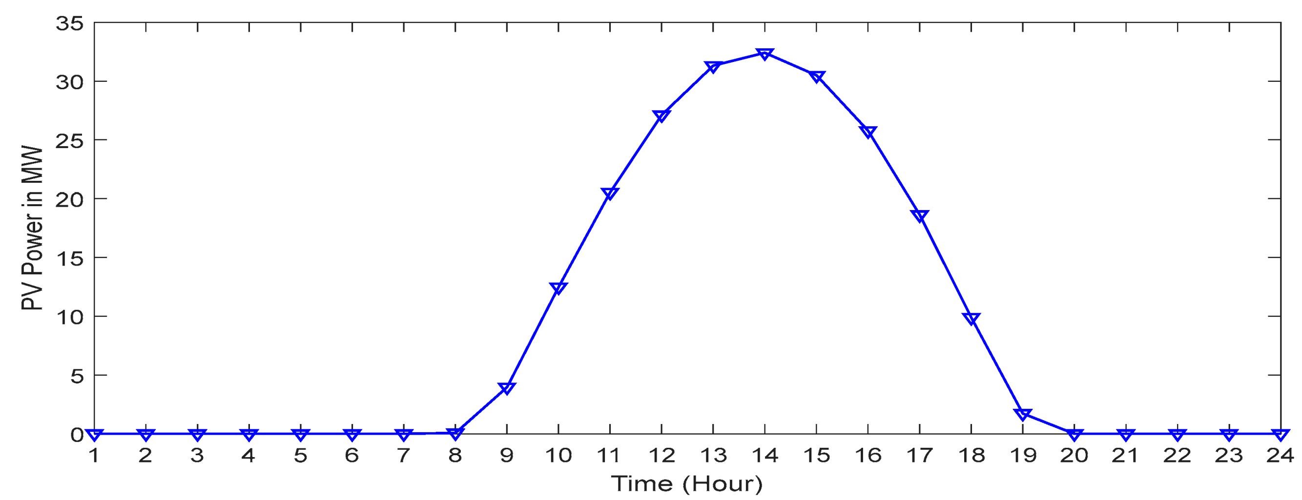
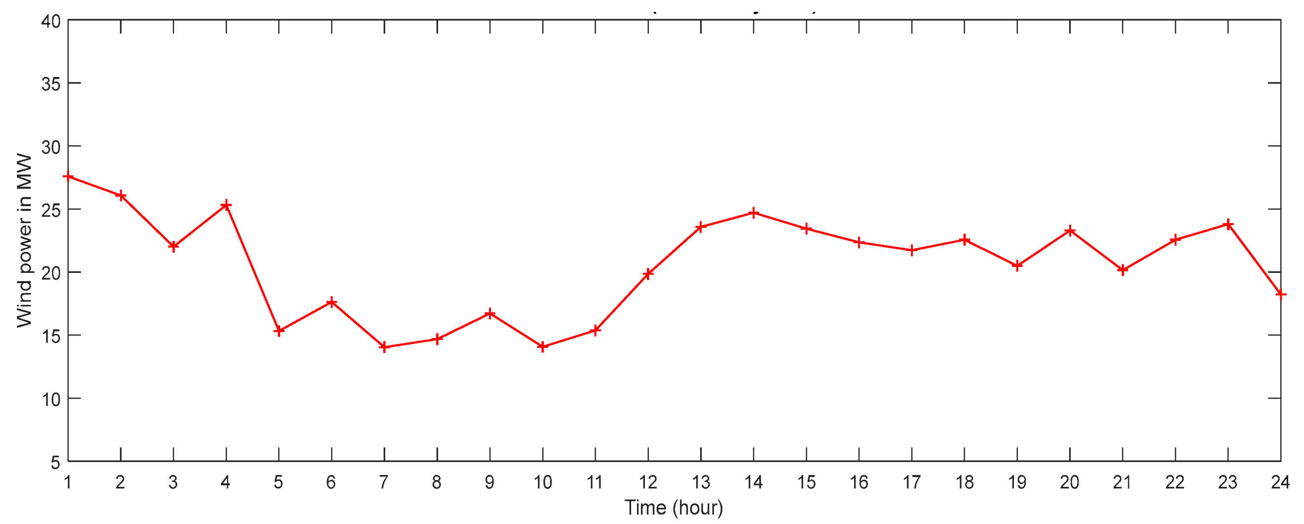
7.2. PV and Wind Data

The Oman Electricity Transmission Company (OETC) provided the wind power statistics utilized in this analysis, which were derived from measurements made in 2022. Oman Power and Water Procurement Company (OPWP) provided the PV data [93]. The PV and wind power datasets were both well documented at hourly intervals. With the help of this systematic process, a solid dataset consisting of 24 separate data points each day was gathered, which allowed for the capture of the power generation fluctuations throughout the day. Figure 6 shows the PV power data for a single day for visual reference. Figure 7 shows the wind power data for a single day, and Figure 8 illustrates the wind power generation for one month to indicate the nature of the wind data. Notable variations in Figure 8 demonstrate how inconsistent the wind power data are. This discrepancy will have an adverse effect on the FFNT training process and the wind power forecast accuracy.

The suggested FFNN is used for forecasting PV and wind power data. The historical data sequence is divided into two sections: training and testing. In particular, the historical data sequence’s first 90% is set aside for the FF neural network model’s training. The network may identify correlations and patterns in the data during this training phase. The trained model is subsequently tested using the remaining 10% of the data, enabling an evaluation of its generalization and predictive ability. The efficacy of the FFNN in forecasting wind power and PV power may be determined by assessing the network’s accuracy with data not from actual observations. The next section presents the simulation results for the suggested FFNN model.

8. Results

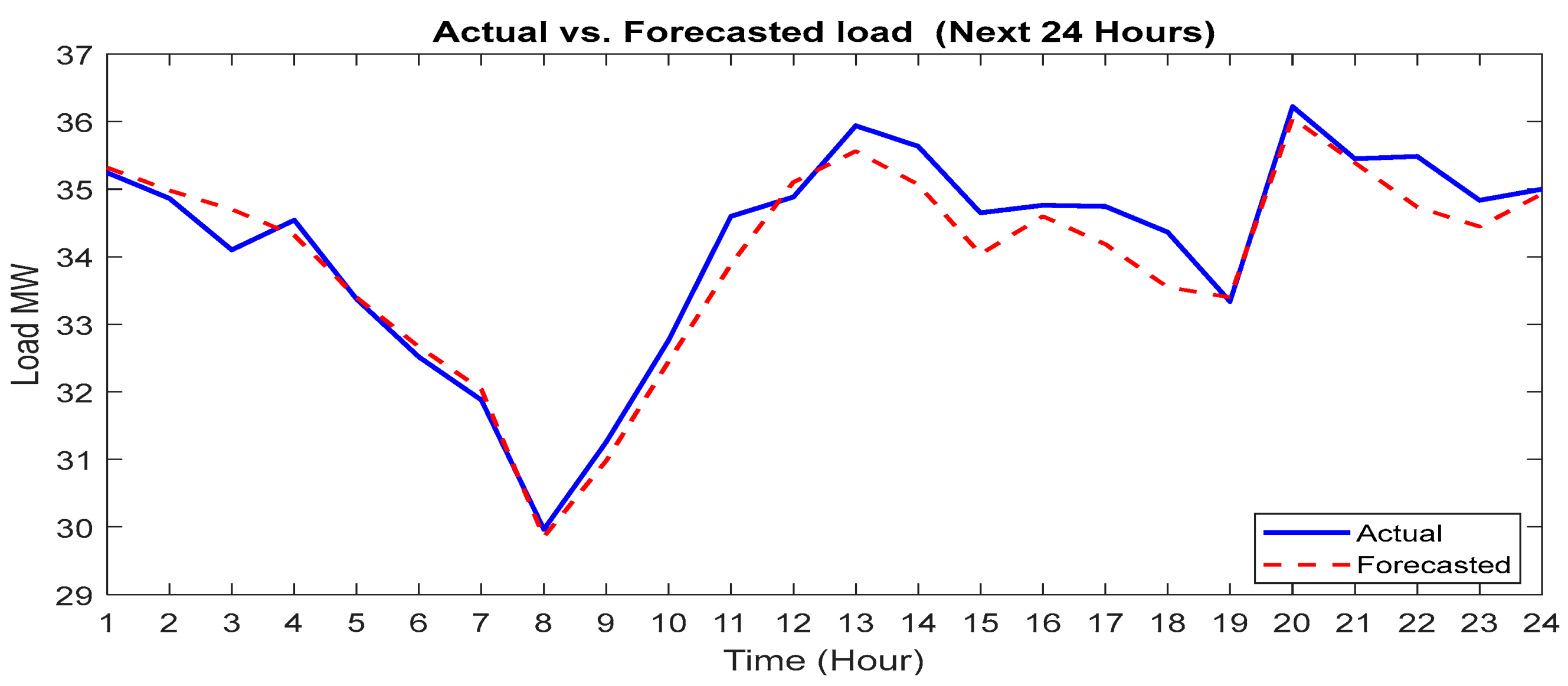
8.1. Load-Power Forecasting Results

Figure 9 presents the results of the forecast study and shows the estimated load power for a subsequent 24 h cycle. The graphical depiction provided by this figure provides a thorough breakdown of the expected fluctuations in load power throughout the course of the following day. By highlighting expected variations from one hour to the next, the representation effectively illustrates the anticipated load-power dynamics. Better planning and management choices based on these forecast insights are made possible by this forecasting, which guarantees a thorough picture of the load power’s expected behavior.

Furthermore, a thorough comparison of the “Actual” values—which represent the observed data—and the “Forecasted” values—which come from predictive analyses—is shown in Figure 9. The “Forecasted” curve closely resembles the size and path of the “Actual” curve, as can be seen by closely examining the curves in Figure 9. The remarkable resemblance between the two curves highlights the great forecasting accuracy. The alignment shows how well the FFNN captures the complex patterns found in the real data, in addition to highlighting the model’s capacity to forecast future trends. This comparison validates the FFNN’s strong forecasting skills and highlights its potential as a dependable instrument for highly accurate load-power prediction.

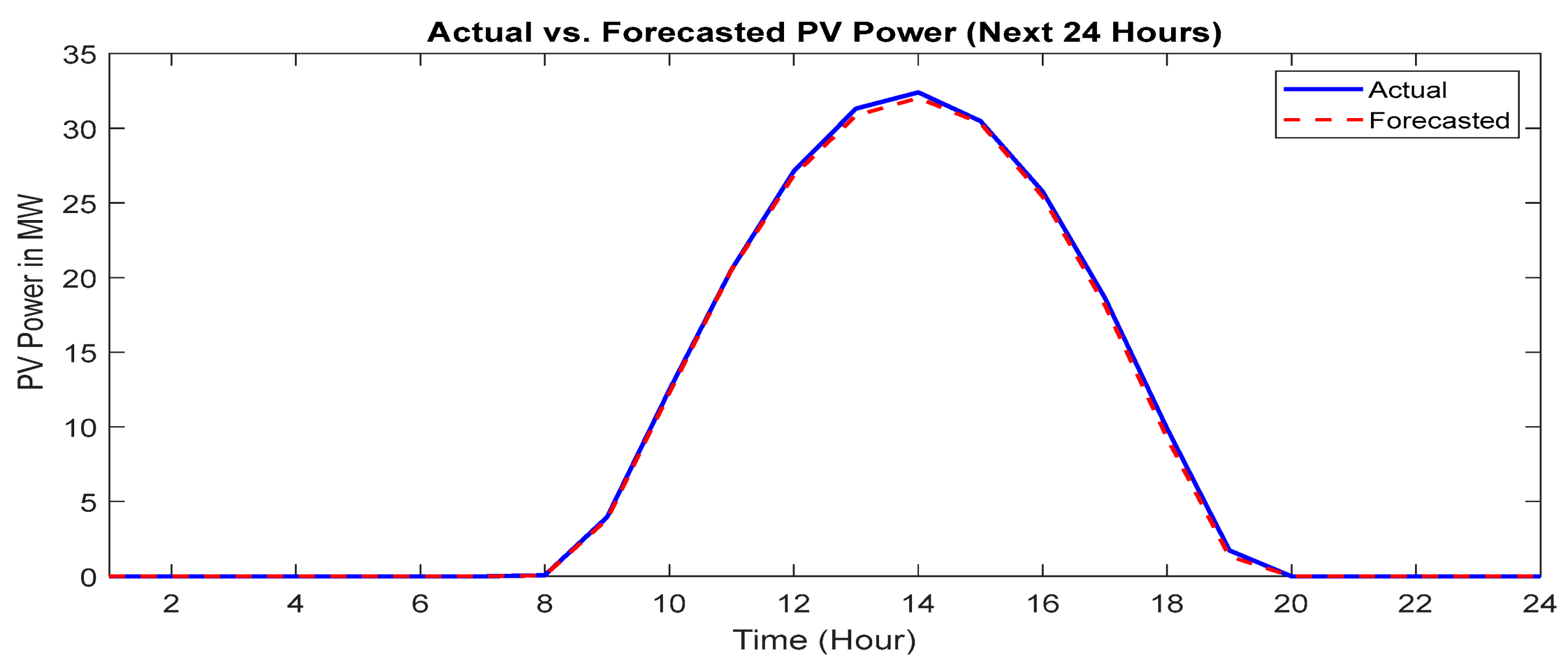
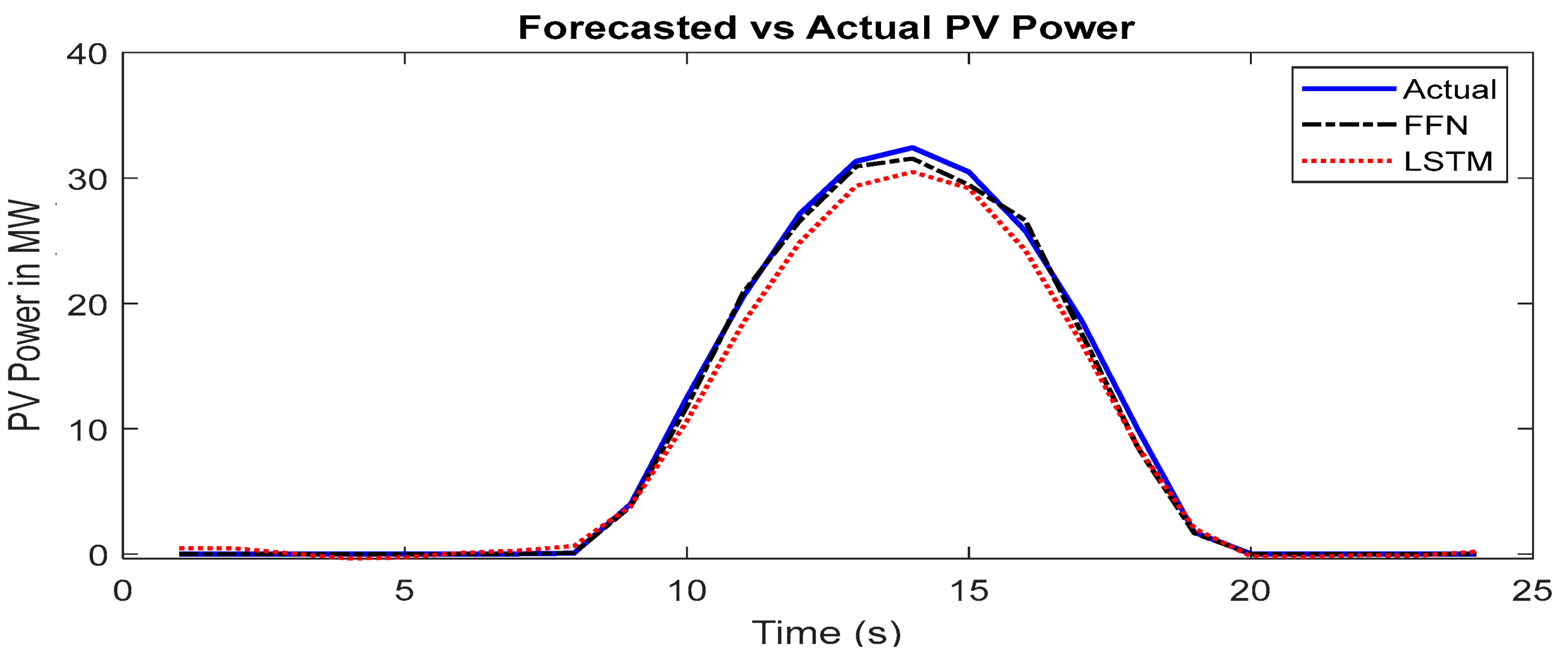
8.2. Wind and PV Power Forecasting Results

The expected values of the wind power for a subsequent 24 h period are graphically represented in Figure 10; this is one of the outputs of the forecasting phase which is displayed in Figure 10 and Figure 11. Similar to Figure 10, Figure 11 shows the predicted PV power generation and provides a visual representation of the forecasted PV output for a subsequent 24 h period. The predicted data in this case start and finish on two distinct days at midnight.

A comparison between the “Actual” values, which show the actual data observed, and the “Forecasted” values, which show the results predicted, is displayed in Figure 9 and Figure 10. It is clear by examining Figure 9 and Figure 10’s curves that the “Forecasted” curve accurately depicts the magnitude and trend of the “Actual” curve. The two curves’ similarity shows that the FFNN has high levels of forecasting capability. Additionally, the findings for wind power forecasting were shown to be not as precise as those of PV power forecasting. The nature of the two signals is responsible for this, due to the smoothness and slower rate of change of the PV data, compared to the wind data. The accuracy of the wind power forecast and the FFNT training procedure are negatively impacted by the previously indicated discrepancy in the wind data.

Furthermore, the suggested approach is compared with Long Short-Term Memory (LSTM) networks in order to evaluate the proposed FFNN. Where LSTM is an efficient way to manage sequences and time-dependent patterns, it is a specific kind of recurrent neural network (RNN). For PV power forecasting, the suggested technique and the LSTM proposed in [85] are tested. Figure 12 displays the simulation results for both approaches. Based on the simulation’s output when LSTM was used to forecast PV power, the results were shown to be less accurate than when FFNN was used. Additionally, LSTM model training takes more time than the suggested FFNN. Furthermore,

Table 4. Comparison between FFNN and LSTM.

Forecast Method	Prediction Standard Deviation	Percentage Difference from Actual Data Standard Deviation (12.3141)
FFNN	12.1647	−1.21%
LSTM	11.5562	−6.15%

displays a comparison between the standard deviations of the FFNN predictions and those of the LSTM predictions, as well as the % difference between the standard deviations of the predictions and the actual data for the standard deviations. With the help of this comparison, it is possible to determine how much the variability in forecasts differs from the variability in the actual data. Notably, compared to the LSTM predictions, the FFNN forecasts had smaller standard-deviation percentage differences. This result indicates that the FFNN model provides predictions with more consistency and accuracy.

Therefore LSTMs are successful in capturing distant relationships, which is crucial for time series forecasting. However, in our specific PV power forecast test, the LSTM model’s performance fell short of that of the FFNN. As a result, the observed advantage of the FFNN model over the LSTM in our investigation emphasizes the significance of taking the issue domain as well as the data characteristics into account when choosing a forecasting approach. While LSTMs are praised for their sequence modeling skills, the FFNN model’s ability to recognize complex patterns in the PV power data allowed it to make predictions that were more accurate. In the end, the precise context and objectives of the prediction job will determine which approach to use: FFNN or LSTM.

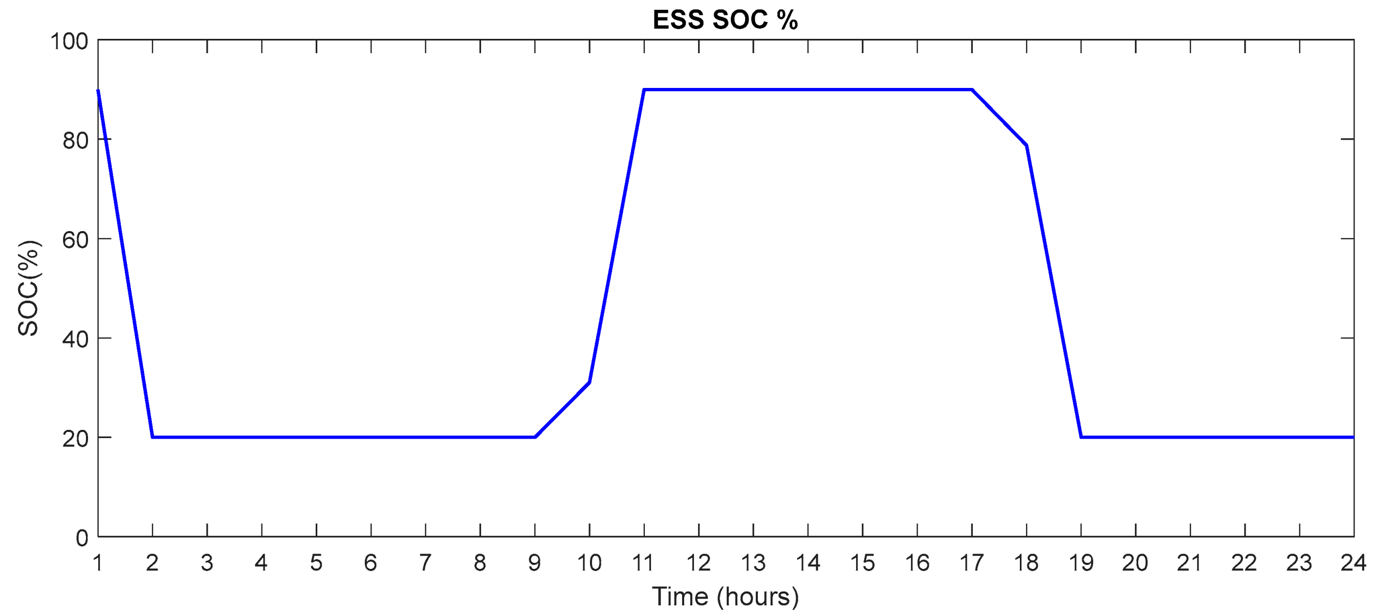
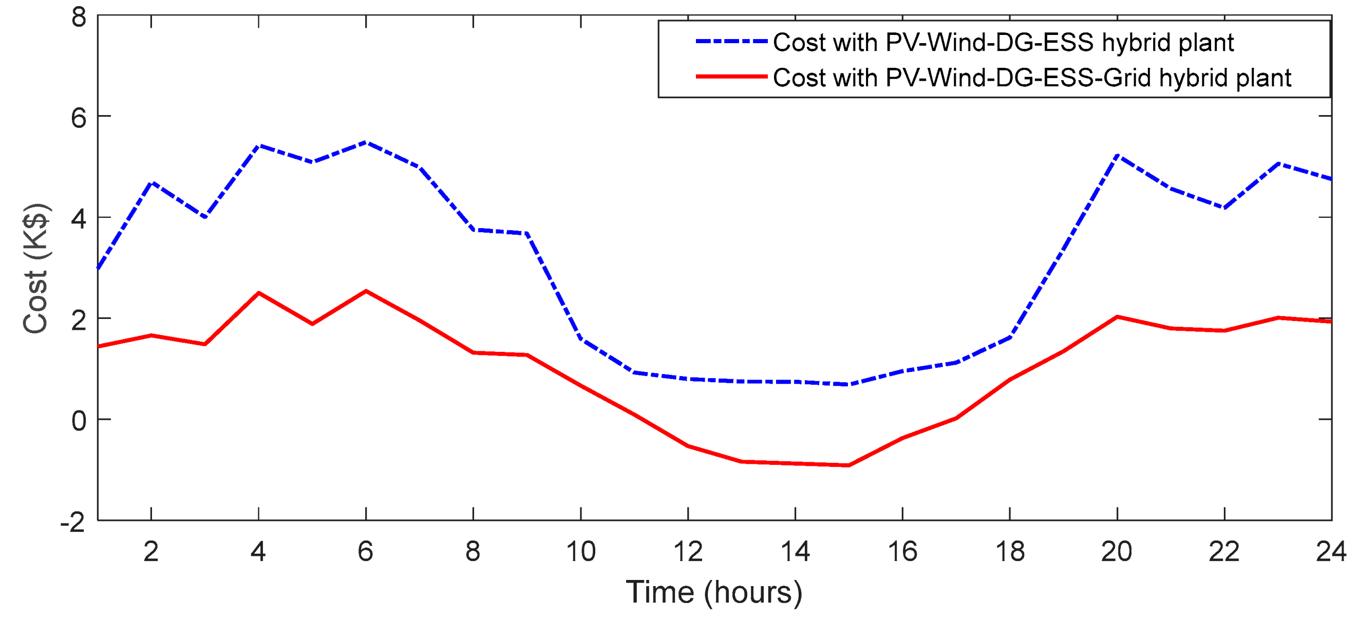
8.3. Dispatch Engine Results

The problem of minimizing the cost in the energy dispatch of the micro-grid using DE, as depicted in Figure 1, has been successfully resolved. This solution is specific to the case study and relies on the utilization of the MILP solver. The results obtained from this approach, demonstrating the optimized energy dispatch and the corresponding minimum cost, are visually presented in Figure 13. Furthermore, the SoC% of the ESS is displayed across the day in Figure 14.

Figure 13 provides a visual representation of the contribution level of each generator element in the microgrid’s energy supply. It illustrates the specific amount of energy that each generator element is required to generate in order to meet the overall energy demand. PV output begins at 8:00 a.m. and increases gradually until noon, when it peaks. Thereafter, it decreases until sunset. In contrast to PV, wind turbine production is unpredictable, since it is based on the wind speed during each hour of the day. The wind generator begins to generate power if the wind speed is greater than the wind turbine’s cut-in wind speed. The PV mostly meets the load demand at noon. The extra wind and PV power is sent to the grid and stored in the ESS between the hours of 10:00 and 17:00, given a suitable amount of wind and PV energy output. When the wind and PV production levels are lower, between the hours of 1:00 and 10:00 and 17:00 and 24:00, the grid and ESS are used to make up for the diminished wind and PV output. It can be observed that by employing this optimization strategy, the utilization of the DG unit is decreased, which lowers plant operating costs, since the DG unit is only operated briefly. Additionally, by connecting the system to the grid, the grid will provide more output to compensate for the system’s insufficient production from wind and PV energy, which will lower the rate at which wind power and PV will be curtailed.

To demonstrate how incorporating the grid affects system regulation performance, a simulation is run for the designed DE utilizing a combination of PV, wind, DG, and ESS facilities. Figure 15 illustrates the variance in hybrid plant running costs between this scenario and the one introduced previously. It is clear that when a system is disconnected from the grid, the DG unit is used more frequently, which raises plant operating costs, since the system’s insufficient output of wind and PV energy cannot be made up for by the grid.

The suggested ED system, however, provides the ability to successfully support islanding operations in the context of real-time support conditions and auxiliary services for hybrid plant dispatch engines, according to the simulation that was given in this example. The proposed ED system has proven its capacity to enable a smooth transition to islanded operation in the case of grid failures or maintenance by tightly integrating advanced control algorithms and responsive data analytics. This accomplishment shows how reliable the proposed strategy is in preserving grid stability and power supply continuity, adding to the necessary range of ancillary services that contemporary hybrid plant dispatch engines work to provide.

9. Conclusions

In order to ensure dispatchable electricity under challenging operating conditions, hybrid power plants have emerged as dependable and adaptable electricity-producing facilities. In order to design and run hybrid power plants, this research suggests implementing a DE based on mixed-integer linear programming (MILP). The DE seeks to minimize operating costs and the reliance on DGs while maintaining the agreed energy output by offering extended-duration operating schedules and facilitating real-time monitoring. The recommended approach includes accurate PV and wind power forecasts, ensuring the best possible scheduling. To assess the feasibility of the proposed dispatch engine, a case study is conducted in Oman, utilizing real-time data from multiple sites in the country for load, wind power, and PV power. Using a hybrid PV–Wind–DG–ESS–Grid plant, the proposed dispatch engine’s performance is assessed, offering helpful insights into the possible advantages and efficiency of the suggested system. The Feed-Forward (FF) neural network is used to forecast data for load, PV power, and wind power, and the findings demonstrate the strong forecasting capabilities of the FF neural network. The implementation results of the proposed DE show how wind and PV energy is sent to the grid and stored in the ESS during peak hours. When production decreases, the grid and ESS compensate. Moreover, the simulation’s results show that using the proposed DE reduces DG unit usage and lowers a plant’s operating costs.

References

1. Kober, T.; Schiffer, H.-W.; Densing, M.; Panos, E. Global energy perspectives to 2060–WEC’s World Energy Scenarios 2019. Energy Strategy Rev. 2020, 31, 100523. [Google Scholar] [CrossRef]
2. Ishraque, M.F.; Shezan, S.A.; Ali, M.; Rashid, M. Optimization of load dispatch strategies for an islanded microgrid connected with renewable energy sources. Appl. Energy 2021, 292, 116879. [Google Scholar] [CrossRef]
3. Mohammed, Y.; Mustafa, M.; Bashir, N. Hybrid renewable energy systems for off-grid electric power: Review of substantial issues. Renew. Sustain. Energy Rev. 2014, 35, 527–539. [Google Scholar] [CrossRef]
4. Bajpai, P.; Dash, V. Hybrid renewable energy systems for power generation in stand-alone applications: A review. Renew. Sustain. Energy Rev. 2012, 16, 2926–2939. [Google Scholar] [CrossRef]
5. Katiraei, F.; Iravani, R.; Hatziargyriou, N.; Dimeas, A. Microgrids management. IEEE Power Energy Mag. 2008, 6, 54–65. [Google Scholar] [CrossRef]
6. Mandal, S.; Das, B.K.; Hoque, N. Optimum sizing of a stand-alone hybrid energy system for rural electrification in Bangladesh. J. Clean. Prod. 2018, 200, 12–27. [Google Scholar] [CrossRef]
7. Baneshi, M.; Hadianfard, F. Techno-economic feasibility of hybrid diesel/PV/wind/battery electricity generation systems for non-residential large electricity consumers under southern Iran climate conditions. Energy Convers. Manag. 2016, 127, 233–244. [Google Scholar] [CrossRef]
8. Mehrpooya, M.; Mohammadi, M.; Ahmadi, E. Techno-economic-environmental study of hybrid power supply system: A case study in Iran. Sustain. Energy Technol. Assess. 2018, 25, 1–10. [Google Scholar]
9. Shezan, S.A.; Julai, S.; Kibria, M.; Ullah, K.; Saidur, R.; Chong, W.; Akikur, R.K. Performance analysis of an off-grid wind-PV (photovoltaic)-diesel-battery hybrid energy system feasible for remote areas. J. Clean. Prod. 2016, 125, 121–132. [Google Scholar] [CrossRef]
10. Hosseini, S.M.; Carli, R.; Dotoli, M. Robust optimal energy management of a residential microgrid under uncertainties on demand and renewable power generation. IEEE Trans. Autom. Sci. Eng. 2020, 18, 618–637. [Google Scholar] [CrossRef]
11. Kakran, S.; Chanana, S. Smart operations of smart grids integrated with distributed generation: A review. Renew. Sustain. Energy Rev. 2018, 81, 524–535. [Google Scholar] [CrossRef]
12. Utkarsh, K.; Srinivasan, D.; Trivedi, A.; Zhang, W.; Reindl, T. Distributed model-predictive real-time optimal operation of a network of smart microgrids. IEEE Trans. Smart Grid 2018, 10, 2833–2845. [Google Scholar] [CrossRef]
13. Qu, B.-Y.; Zhu, Y.; Jiao, Y.; Wu, M.; Suganthan, P.N.; Liang, J.J. A survey on multi-objective evolutionary algorithms for the solution of the environmental/economic dispatch problems. Swarm Evol. Comput. 2018, 38, 1–11. [Google Scholar] [CrossRef]
14. Xiong, G.; Shi, D.; Duan, X. Multi-strategy ensemble biogeography-based optimization for economic dispatch problems. Appl. Energy 2013, 111, 801–811. [Google Scholar] [CrossRef]
15. Ellahi, M.; Abbas, G.; Khan, I.; Koola, P.M.; Nasir, M.; Raza, A.; Farooq, U. Recent approaches of forecasting and optimal economic dispatch to overcome intermittency of wind and photovoltaic (PV) systems: A review. Energies 2019, 12, 4392. [Google Scholar] [CrossRef]
16. Xia, H.; Li, Q.; Xu, R.; Chen, T.; Wang, J.; Hassan, M.A.S.; Chen, M. Distributed control method for economic dispatch in islanded microgrids with renewable energy sources. IEEE Access 2018, 6, 21802–21811. [Google Scholar] [CrossRef]
17. Tang, Z.; Hill, D.J.; Liu, T. A novel consensus-based economic dispatch for microgrids. IEEE Trans. Smart Grid 2018, 9, 3920–3922. [Google Scholar] [CrossRef]
18. Yang, S.; Tan, S.; Xu, J.-X. Consensus based approach for economic dispatch problem in a smart grid. IEEE Trans. Power Syst. 2013, 28, 4416–4426. [Google Scholar] [CrossRef]
19. Reddy, S.S.; Bijwe, P.; Abhyankar, A.R. Real-time economic dispatch considering renewable power generation variability and uncertainty over scheduling period. IEEE Syst. J. 2014, 9, 1440–1451. [Google Scholar] [CrossRef]
20. Muttaqi, K.M.; Sutanto, D. An effective power dispatch strategy to improve generation schedulability by mitigating wind power uncertainty with a data driven flexible dispatch margin for a wind farm using a multi-unit battery energy storage system. In Proceedings of the 2018 IEEE Industry Applications Society Annual Meeting (IAS), Portland, OR, USA, 23–27 September 2018; pp. 1–8. [Google Scholar]
21. Ye, L.; Zhang, C.; Tang, Y.; Zhong, W.; Zhao, Y.; Lu, P.; Zhai, B.; Lan, H.; Li, Z. Hierarchical model predictive control strategy based on dynamic active power dispatch for wind power cluster integration. IEEE Trans. Power Syst. 2019, 34, 4617–4629. [Google Scholar] [CrossRef]
22. Arefin, S.S. Optimization techniques of islanded hybrid microgrid system. In Renewable Energy-Resources, Challenges and Applications; IntechOpen: London, UK, 2020. [Google Scholar]
23. Chauhan, A.; Saini, R. A review on Integrated Renewable Energy System based power generation for stand-alone applications: Configurations, storage options, sizing methodologies and control. Renew. Sustain. Energy Rev. 2014, 38, 99–120. [Google Scholar] [CrossRef]
24. Husein, M.; Chung, I.-Y. Optimal design and financial feasibility of a university campus microgrid considering renewable energy incentives. Appl. Energy 2018, 225, 273–289. [Google Scholar] [CrossRef]
25. Mazzola, S.; Astolfi, M.; Macchi, E. The potential role of solid biomass for rural electrification: A techno economic analysis for a hybrid microgrid in India. Appl. Energy 2016, 169, 370–383. [Google Scholar] [CrossRef]
26. Mazzola, S.; Vergara, C.; Astolfi, M.; Li, V.; Perez-Arriaga, I.; Macchi, E. Assessing the value of forecast-based dispatch in the operation of off-grid rural microgrids. Renew. Energy 2017, 108, 116–125. [Google Scholar] [CrossRef]
27. Moretti, L.; Astolfi, M.; Vergara, C.; Macchi, E.; Pérez-Arriaga, J.I.; Manzolini, G. A design and dispatch optimization algorithm based on mixed integer linear programming for rural electrification. Appl. Energy 2019, 233, 1104–1121. [Google Scholar] [CrossRef]
28. Ferrer-Martí, L.; Domenech, B.; García-Villoria, A.; Pastor, R. A MILP model to design hybrid wind–photovoltaic isolated rural electrification projects in developing countries. Eur. J. Oper. Res. 2013, 226, 293–300. [Google Scholar] [CrossRef]
29. Mehleri, E.D.; Sarimveis, H.; Markatos, N.C.; Papageorgiou, L.G. Optimal design and operation of distributed energy systems: Application to Greek residential sector. Renew. Energy 2013, 51, 331–342. [Google Scholar] [CrossRef]
30. Moretti, L.; Polimeni, S.; Meraldi, L.; Raboni, P.; Leva, S.; Manzolini, G. Assessing the impact of a two-layer predictive dispatch algorithm on design and operation of off-grid hybrid microgrids. Renew. Energy 2019, 143, 1439–1453. [Google Scholar] [CrossRef]
31. Dagnachew, A.G.; Lucas, P.L.; Hof, A.F.; Gernaat, D.E.; de Boer, H.-S.; van Vuuren, D.P. The role of decentralized systems in providing universal electricity access in Sub-Saharan Africa–A model-based approach. Energy 2017, 139, 184–195. [Google Scholar] [CrossRef]
32. Renewable, H.-H. Distributed Generation System Design Software. 2017. Available online: http://homerenergy.com (accessed on 18 April 2023).
33. Eriksson, E.; Gray, E.M. Optimization and integration of hybrid renewable energy hydrogen fuel cell energy systems–A critical review. Appl. Energy 2017, 202, 348–364. [Google Scholar] [CrossRef]
34. Barley, C.D.; Winn, C.B. Optimal dispatch strategy in remote hybrid power systems. Sol. Energy 1996, 58, 165–179. [Google Scholar] [CrossRef]
35. Ammari, C.; Belatrache, D.; Touhami, B.; Makhloufi, S. Sizing, optimization, control and energy management of hybrid renewable energy system—A review. Energy Built Environ. 2021, 3, 399–411. [Google Scholar] [CrossRef]
36. Al-Falahi, M.D.; Jayasinghe, S.; Enshaei, H. A review on recent size optimization methodologies for standalone solar and wind hybrid renewable energy system. Energy Convers. Manag. 2017, 143, 252–274. [Google Scholar] [CrossRef]
37. Siddaiah, R.; Saini, R. A review on planning, configurations, modeling and optimization techniques of hybrid renewable energy systems for off grid applications. Renew. Sustain. Energy Rev. 2016, 58, 376–396. [Google Scholar] [CrossRef]
38. Vaccari, M.; Mancuso, G.; Riccardi, J.; Cantù, M.; Pannocchia, G. A sequential linear programming algorithm for economic optimization of hybrid renewable energy systems. J. Process Control 2019, 74, 189–201. [Google Scholar] [CrossRef]
39. Chang, C.-T. Multi-choice goal programming model for the optimal location of renewable energy facilities. Renew. Sustain. Energy Rev. 2015, 41, 379–389. [Google Scholar] [CrossRef]
40. Ming, M.; Wang, R.; Zha, Y.; Zhang, T. Multi-objective optimization of hybrid renewable energy system using an enhanced multi-objective evolutionary algorithm. Energies 2017, 10, 674. [Google Scholar] [CrossRef]
41. Wang, R.; Li, G.; Ming, M.; Wu, G.; Wang, L. An efficient multi-objective model and algorithm for sizing a stand-alone hybrid renewable energy system. Energy 2017, 141, 2288–2299. [Google Scholar] [CrossRef]
42. Nemati, M.; Braun, M.; Tenbohlen, S. Optimization of unit commitment and economic dispatch in microgrids based on genetic algorithm and mixed integer linear programming. Appl. Energy 2018, 210, 944–963. [Google Scholar] [CrossRef]
43. Wu, N.; Wang, H. Deep learning adaptive dynamic programming for real time energy management and control strategy of micro-grid. J. Clean. Prod. 2018, 204, 1169–1177. [Google Scholar] [CrossRef]
44. Das, B.; Kumar, A. A NLP approach to optimally size an energy storage system for proper utilization of renewable energy sources. Procedia Comput. Sci. 2018, 125, 483–491. [Google Scholar] [CrossRef]
45. Derrouazin, A.; Aillerie, M.; Mekkakia-Maaza, N.; Charles, J.-P. Multi input-output fuzzy logic smart controller for a residential hybrid solar-wind-storage energy system. Energy Convers. Manag. 2017, 148, 238–250. [Google Scholar] [CrossRef]
46. Suganthi, L.; Iniyan, S.; Samuel, A.A. Applications of fuzzy logic in renewable energy systems–a review. Renew. Sustain. Energy Rev. 2015, 48, 585–607. [Google Scholar] [CrossRef]
47. Athari, M.; Ardehali, M. Operational performance of energy storage as function of electricity prices for on-grid hybrid renewable energy system by optimized fuzzy logic controller. Renew. Energy 2016, 85, 890–902. [Google Scholar] [CrossRef]
48. Mahmoudi, S.M.; Maleki, A.; Ochbelagh, D.R. Optimization of a hybrid energy system with/without considering back-up system by a new technique based on fuzzy logic controller. Energy Convers. Manag. 2021, 229, 113723. [Google Scholar] [CrossRef]
49. Mayer, M.J.; Szilágyi, A.; Gróf, G. Environmental and economic multi-objective optimization of a household level hybrid renewable energy system by genetic algorithm. Appl. Energy 2020, 269, 115058. [Google Scholar] [CrossRef]
50. Das, B.K.; Hassan, R.; Tushar, M.S.H.; Zaman, F.; Hasan, M.; Das, P. Techno-economic and environmental assessment of a hybrid renewable energy system using multi-objective genetic algorithm: A case study for remote Island in Bangladesh. Energy Convers. Manag. 2021, 230, 113823. [Google Scholar] [CrossRef]
51. Abdelkader, A.; Rabeh, A.; Ali, D.M.; Mohamed, J. Multi-objective genetic algorithm based sizing optimization of a stand-alone wind/PV power supply system with enhanced battery/supercapacitor hybrid energy storage. Energy 2018, 163, 351–363. [Google Scholar] [CrossRef]
52. Lü, X.; Wu, Y.; Lian, J.; Zhang, Y.; Chen, C.; Wang, P.; Meng, L. Energy management of hybrid electric vehicles: A review of energy optimization of fuel cell hybrid power system based on genetic algorithm. Energy Convers. Manag. 2020, 205, 112474. [Google Scholar] [CrossRef]
53. Javed, M.S.; Song, A.; Ma, T. Techno-economic assessment of a stand-alone hybrid solar-wind-battery system for a remote island using genetic algorithm. Energy 2019, 176, 704–717. [Google Scholar] [CrossRef]
54. Rahman, M.M.; Shakeri, M.; Tiong, S.K.; Khatun, F.; Amin, N.; Pasupuleti, J.; Hasan, M.K. Prospective methodologies in hybrid renewable energy systems for energy prediction using artificial neural networks. Sustainability 2021, 13, 2393. [Google Scholar] [CrossRef]
55. Amirtharaj, S.; Premalatha, L.; Gopinath, D. Optimal utilization of renewable energy sources in MG connected system with integrated converters: An AGONN Approach. Analog Integr. Circuits Signal Process. 2019, 101, 513–532. [Google Scholar] [CrossRef]
56. Azaza, M.; Wallin, F. Multi objective particle swarm optimization of hybrid micro-grid system: A case study in Sweden. Energy 2017, 123, 108–118. [Google Scholar] [CrossRef]
57. Shang, C.; Srinivasan, D.; Reindl, T. An improved particle swarm optimisation algorithm applied to battery sizing for stand-alone hybrid power systems. Int. J. Electr. Power Energy Syst. 2016, 74, 104–117. [Google Scholar] [CrossRef]
58. Elsheikh, A.; Elaziz, M.A. Review on applications of particle swarm optimization in solar energy systems. Int. J. Environ. Sci. Technol. 2019, 16, 1159–1170. [Google Scholar] [CrossRef]
59. Yaïci, W.; Entchev, E. Adaptive Neuro-Fuzzy Inference System modelling for performance prediction of solar thermal energy system. Renew. Energy 2016, 86, 302–315. [Google Scholar] [CrossRef]
60. Dawan, P.; Sriprapha, K.; Kittisontirak, S.; Boonraksa, T.; Junhuathon, N.; Titiroongruang, W.; Niemcharoen, S. Comparison of power output forecasting on the photovoltaic system using adaptive neuro-fuzzy inference systems and particle swarm optimization-artificial neural network model. Energies 2020, 13, 351. [Google Scholar] [CrossRef]
61. Chen, Y.; Chen, C.; Ma, J.; Qiu, W.; Liu, S.; Lin, Z.; Qian, M.; Zhu, L.; Zhao, D. Multi-objective optimization strategy of multi-sources power system operation based on fuzzy chance constraint programming and improved analytic hierarchy process. Energy Rep. 2021, 7, 268–274. [Google Scholar] [CrossRef]
62. Algarín, C.R. An analytic hierarchy process based approach for evaluating renewable energy sources. Int. J. Energy Econ. Policy 2017, 7, 38–47. [Google Scholar]
63. Saharia, B.J.; Brahma, H.; Sarmah, N. A review of algorithms for control and optimization for energy management of hybrid renewable energy systems. J. Renew. Sustain. Energy 2018, 10, 053502. [Google Scholar] [CrossRef]
64. Wang, Q.; Yang, X. Investigating the sustainability of renewable energy–An empirical analysis of European Union countries using a hybrid of projection pursuit fuzzy clustering model and accelerated genetic algorithm based on real coding. J. Clean. Prod. 2020, 268, 121940. [Google Scholar] [CrossRef]
65. Sadeghi, A.; Larimian, T. Sustainable electricity generation mix for Iran: A fuzzy analytic network process approach. Sustain. Energy Technol. Assess. 2018, 28, 30–42. [Google Scholar] [CrossRef]
66. Dhiman, H.S.; Deb, D. Fuzzy TOPSIS and fuzzy COPRAS based multi-criteria decision making for hybrid wind farms. Energy 2020, 202, 117755. [Google Scholar] [CrossRef]
67. Diemuodeke, E.; Addo, A.; Oko, C.; Mulugetta, Y.; Ojapah, M. Optimal mapping of hybrid renewable energy systems for locations using multi-criteria decision-making algorithm. Renew. Energy 2019, 134, 461–477. [Google Scholar] [CrossRef]
68. Kumar, M.R.; Ghosh, S.; Das, S. Frequency dependent piecewise fractional-order modelling of ultracapacitors using hybrid optimization and fuzzy clustering. J. Power Sources 2016, 335, 98–104. [Google Scholar] [CrossRef]
69. Zhang, G.; Wu, B.; Maleki, A.; Zhang, W. Simulated annealing-chaotic search algorithm based optimization of reverse osmosis hybrid desalination system driven by wind and solar energies. Sol. Energy 2018, 173, 964–975. [Google Scholar] [CrossRef]
70. Zhang, W.; Maleki, A.; Rosen, M.A.; Liu, J. Sizing a stand-alone solar-wind-hydrogen energy system using weather forecasting and a hybrid search optimization algorithm. Energy Convers. Manag. 2019, 180, 609–621. [Google Scholar] [CrossRef]
71. Zhang, W.; Maleki, A.; Rosen, M.A.; Liu, J. Optimization with a simulated annealing algorithm of a hybrid system for renewable energy including battery and hydrogen storage. Energy 2018, 163, 191–207. [Google Scholar] [CrossRef]
72. Gu, Y.; Zhang, X.; Myhren, J.A.; Han, M.; Chen, X.; Yuan, Y. Techno-economic analysis of a solar photovoltaic/thermal (PV/T) concentrator for building application in Sweden using Monte Carlo method. Energy Convers. Manag. 2018, 165, 8–24. [Google Scholar] [CrossRef]
73. Ghorbani, N.; Kasaeian, A.; Toopshekan, A.; Bahrami, L.; Maghami, A. Optimizing a hybrid wind-PV-battery system using GA-PSO and MOPSO for reducing cost and increasing reliability. Energy 2018, 154, 581–591. [Google Scholar] [CrossRef]
74. Heydari, A.; Garcia, D.A.; Keynia, F.; Bisegna, F.; De Santoli, L. A novel composite neural network based method for wind and solar power forecasting in microgrids. Appl. Energy 2019, 251, 113353. [Google Scholar] [CrossRef]
75. Oman Power and Water Procurement. 2019. Available online: https://omanpwp.om/chart-fuel-diversification-policy (accessed on 22 June 2023).
76. Oman, O.V.D. 2040 Vision Office. 2019. Available online: https://www.national-day-of-oman.info/wp-content/uploads/2020/11/OmanVision2040-Preliminary-Vision-Document.pdf (accessed on 2 July 2023).
77. Borisoot, K.; Liemthong, R.; Srithapon, C.; Chatthaworn, R. Optimal energy management for virtual power plant considering operation and degradation costs of energy storage system and generators. Energies 2023, 16, 2862. [Google Scholar] [CrossRef]
78. Fathy, A.; Kaaniche, K.; Alanazi, T.M. Recent approach based social spider optimizer for optimal sizing of hybrid PV/wind/battery/diesel integrated microgrid in aljouf region. IEEE Access 2020, 8, 57630–57645. [Google Scholar] [CrossRef]
79. Ayop, R.; Tan, C.W. A comprehensive review on photovoltaic emulator. Renew. Sustain. Energy Rev. 2017, 80, 430–452. [Google Scholar] [CrossRef]
80. Belboul, Z.; Toual, B.; Kouzou, A.; Mokrani, L.; Bensalem, A.; Kennel, R.; Abdelrahem, M. Multiobjective optimization of a hybrid PV/Wind/Battery/Diesel generator system integrated in microgrid: A case study in Djelfa, Algeria. Energies 2022, 15, 3579. [Google Scholar] [CrossRef]
81. Nadjemi, O.; Nacer, T.; Hamidat, A.; Salhi, H. Optimal hybrid PV/wind energy system sizing: Application of cuckoo search algorithm for Algerian dairy farms. Renew. Sustain. Energy Rev. 2017, 70, 1352–1365. [Google Scholar] [CrossRef]
82. Dong, W.; Li, Y.; Xiang, J. Optimal sizing of a stand-alone hybrid power system based on battery/hydrogen with an improved ant colony optimization. Energies 2016, 9, 785. [Google Scholar] [CrossRef]
83. Rao, S.S. Engineering Optimization: Theory; John Wiley & Sons: Hoboken, NJ, USA, 2019. [Google Scholar]
84. Hu, Y.; Li, Y.; Xu, M.; Zhou, L.; Cui, M. A chance-constrained economic dispatch model in wind-thermal-energy storage system. Energies 2017, 10, 326. [Google Scholar] [CrossRef]
85. Liu, X.; Li, X.; Tian, J.; Wang, Y.; Xiao, G.; Wang, P. Day-Ahead Economic Dispatch of Renewable Energy System considering Wind and Photovoltaic Predicted Output. Int. Trans. Electr. Energy Syst. 2022, 2022, 6082642. [Google Scholar] [CrossRef]
86. Ma, J.; Ma, X. A review of forecasting algorithms and energy management strategies for microgrids. Syst. Sci. Control Eng. 2018, 6, 237–248. [Google Scholar] [CrossRef]
87. Vielma, J.P. Mixed integer linear programming formulation techniques. Siam Rev. 2015, 57, 3–57. [Google Scholar] [CrossRef]
88. Smith, J.C.; Taskin, Z.C. A tutorial guide to mixed-integer programming models and solution techniques. Optim. Med. Biol. 2008, 521–548. [Google Scholar]
89. Ren, Y.; Suganthan, P.; Srikanth, N. Ensemble methods for wind and solar power forecasting—A state-of-the-art review. Renew. Sustain. Energy Rev. 2015, 50, 82–91. [Google Scholar] [CrossRef]
90. Abuella, M.; Chowdhury, B. Solar power forecasting using artificial neural networks. In Proceedings of the 2015 North American Power Symposium (NAPS), Charlotte, NC, USA, 4–6 October 2015; pp. 1–5. [Google Scholar]
91. Sharma, V.; Rai, S.; Dev, A. A comprehensive study of artificial neural networks. Int. J. Adv. Res. Comput. Sci. Softw. Eng. 2012, 2, 278–284. [Google Scholar]
92. International Renewable Energy Agency (IRENA). 2021. Available online: https://www.irena.org/Energy-Transition/Technology/Power-generation-costs (accessed on 27 October 2023).
93. Oman Power and Water Procurement (OPWP). Available online: https://omanpwp.om/solar-resource-data (accessed on 2 November 2023).
Figure 1. Dispatch engine.
Energies 17 03281 g001
Figure 2. EMS algorithm flowchart.
Energies 17 03281 g002
Figure 3. Branch-and-bound tree.
Energies 17 03281 g003
Figure 4. Feed-forward neural networks.
Energies 17 03281 g004
Figure 5. Load data.
Energies 17 03281 g005
Figure 6. PV power data for one day.
Energies 17 03281 g006
Figure 7. Wind power data for one day.
Energies 17 03281 g007
Figure 8. Wind power data for one month.
Energies 17 03281 g008
Figure 9. Forecast of wind power.
Energies 17 03281 g009
Figure 10. Forecast of wind power.
Energies 17 03281 g010
Figure 11. Forecast of PV power.
Energies 17 03281 g011
Figure 12. FFNN and LSTM forecasting.
Energies 17 03281 g012
Figure 13. Dispatch of each generator for a PV–Wind–DG–ESS–Grid hybrid plant.
Energies 17 03281 g013
Figure 14. ESS SoC%.
Energies 17 03281 g014
Figure 15. Hybrid plant operating costs for different optimal dispatch cases.
Energies 17 03281 g015