Research on Variable Speed Variable Displacement Power Unit with High Efficiency and High Dynamic Optimized Matching

Abstract

For the variable speed variable displacement power unit (VSVDPU), achieving power matching between the permanent magnet synchronous motor (PMSM) and the variable displacement plunger pump (VDPP) is the key to reducing system energy consumption. The control method of adjusting the speed of the PMSM and the displacement of the VDPP is the mainstay of current research and application of the VSVDPU. However, the dynamic properties of the PMSM and VDPP have not been balanced, which affects the control effect of the VSVDPU. This paper proposes a control method of variable speed and variable displacement with low energy consumption and high dynamics. The main idea is based on the efficiency model and dynamic response model of the PMSM and VDPP, and the factors that affect the efficiency and dynamic characteristics of the VSVDPU are analyzed. Guided by the multi-objective optimization algorithm, the optimal combination of speed and displacement under specific working conditions is derived. Simulation and experiment results show that the proposed control method is feasible to improve the efficiency and dynamic characteristics of the VSVDPU.

1. Introduction

The volumetric speed control system is a hydraulic system that realizes the speed control of the actuator by adjusting the motor speed or the displacement of the hydraulic pump [1,2]. Compared with the throttle speed control system, it has the advantages of high efficiency, energy saving, high power to weight ratio, etc., and is widely used in aerospace, marine power, industrial automation, wind power variable pitch control, and other fields [3,4,5,6].

As the core component in the volumetric speed control system, the electro-hydraulic power unit (EHPU) can accurately respond to system commands to achieve high-precision motion control [7]. In the volumetric speed control system, there are three EHPU combination schemes as follows: variable speed fixed displacement power unit (VSFDPU), fixed speed variable displacement power unit (FSVDPU), and variable speed variable displacement power unit (VSVDPU), as shown in Figure 1.

(a) VSFDPU: This configuration can adjust the flow rate through speed regulation, and then adjust the output power, lowering energy consumption; however, when the working condition changes dramatically, the load demand power changes over a wide range, causing the dynamic response requirements to increase and making it difficult for the VSFDPU to meet the needs of the frequent speed changes.

(b) FSVDPU: This configuration can adjust the flow rate through displacement regulation, thereby changing the output power. Compared to the VSFDPU, it has better dynamic characteristics. However, the motor needs to maintain a rated speed during operation, which generates a large amount of heat and results in lower efficiency.

(c) VSVDPU: This configuration achieves power matching through combined control of speed and displacement. During system operation, the permanent magnet synchronous motor (PMSM) speed and the variable displacement plunger pump (VDPP) displacement can be dynamically adjusted based on the load power demand, improving system efficiency while reducing noise and heat generation.

Compared with the VSFDPU and the FSVDPU, since the VSVDPU can quickly respond to load changes and maintain efficient energy conversion, it can maintain stable output performance under various working conditions [8,9,10,11]. Based on the above analysis, the VSVDPU of the VDPP driven by the PMSM was taken as the research object in this paper.

In pursuit of high efficiency and good dynamic performance for the VSVDPU, the effect of the interaction between the PMSM and VDPP on the performance of the VSVDPU needs to be further investigated [12,13,14]. At present, matching the speed of the PMSM and the displacement of the VDPP to further reduce the energy consumption of the whole machine is a technical problem [15]. Experts and scholars in the industry have conducted research on the power matching of the VSVDPU configuration.

Cecchin Leonardo et al. compared the model predictive controller with the reference controller of the bivariate system on both simulations and test benches, demonstrating its potential in terms of efficiency and flow-tracking dynamics [16]. Willkomm Johannes et al. established a mathematical model for the dynamic response of power units with variable speed and displacement and obtained the optimal speed and discharge values for flow response under varying operating conditions through a novel process adaptation control concept. Then, a mathematical model of dynamic loss of bivariable power units was established, and a control method of model prediction was proposed. In the highly dynamic process cycle, the proposed optimal control method ensured the best energy efficiency [17]. Jin Rui et al. proposed an AI-enabled energy-saving strategy (AIESS), which aimed to achieve efficient hydraulic systems. The strategy integrated the extreme gradient enhancement algorithm (XGBoost) and genetic algorithm (GA) to optimize the real-time control of the variable pump drive system (SDVP) to accurately predict the input power of SDVP and optimize the total energy consumption [18]. Zhang Ye et al. introduced an optimal control method, based on feedback linearization, to improve the dual input single output (DISO) nonlinear speed monitoring problem in electro-hydraulic vibration servo pump (EHA-PVPM) systems [19]. Francois Malrai et al. proposed an original electrical energy optimization method aimed at minimizing electrical energy consumption during pump system operation. The study used variable speed drives (VSD) to simulate both single- and multi-pump systems and demonstrated that the proposed optimization solution is equivalent to minimizing pump losses [20]. Kim et al. achieved constant system pressure by simultaneously controlling the motor speed and the displacement of the hydraulic pump, and this significantly reduced the output power of the system under idle conditions compared with the traditional constant-pressure variable pump driven at constant speed [21]. Assaf et al. discussed the differences in efficiency, quality, and compactness of motor pumps with three architectures of constant speed and variable displacement, variable speed, and variable displacement, among which variable speed and variable displacement had the highest efficiency [22]. Brecher Christian et al. designed a new type of energy-saving hydraulic device for the machine tool, combining the bivariable power unit and the hydraulic booster, reducing the overall energy consumption and operating temperature of the machine tool [23]. Huang Haihong et al. used a power unit with variable speed and displacement on a hydraulic press, obtained the speed and discharge values corresponding to the best efficiency under different load conditions by testing and compiled a lookup table, adopted the energy-saving control strategy of subsection search, and effectively improved the overall energy efficiency of the power unit. Then, the energy efficiency of the variable speed and displacement power unit in the process of state change was studied, then the boundary conditions and energy efficiency model of the system stability when the speed and displacement change were given, and the motor acceleration with the minimum dynamic energy consumption was obtained [24]. Yan Zheng et al. replaced the traditional variable pump with the power source of a variable pressure pump driven by a variable frequency motor, realized the functions of constant pressure, constant flow, and constant power, and effectively reduced the output power of the motor under high pressure and low flow and idle conditions [25].

The above research on the VSVDPU does not consider the efficiency characteristics of PMSM and VDPP, only taking into account the dynamic characteristics of the PMSM speed and the VDPP displacement. The VSVDPU matching method that takes into account both low energy consumption and high dynamics needs further research.

This paper took the VSVDPU as the subject of study and established mathematical models to describe the dynamic response and efficiency of the PMSM and VDPP. It revealed the coupling mechanism between rotational speed, displacement, and pressure on the efficiency and dynamic response of the VSVDPU. The optimization target function was established for the dynamic response and energy efficiency of the VSVDPU. Simulation research was conducted to explore the high-efficiency and high-dynamic control method of the VSVDPU, based on the multi-objective particle swarm optimization algorithm. Additionally, the experimental platform was set up to conduct experiments on the matching effect between the rotational speed and displacement of the VSVDPU, further verifying the accuracy and feasibility of the multi-objective particle swarm optimization control method for the VSVDPU.

2. Dynamic Characteristic Analysis of the VSVDPU

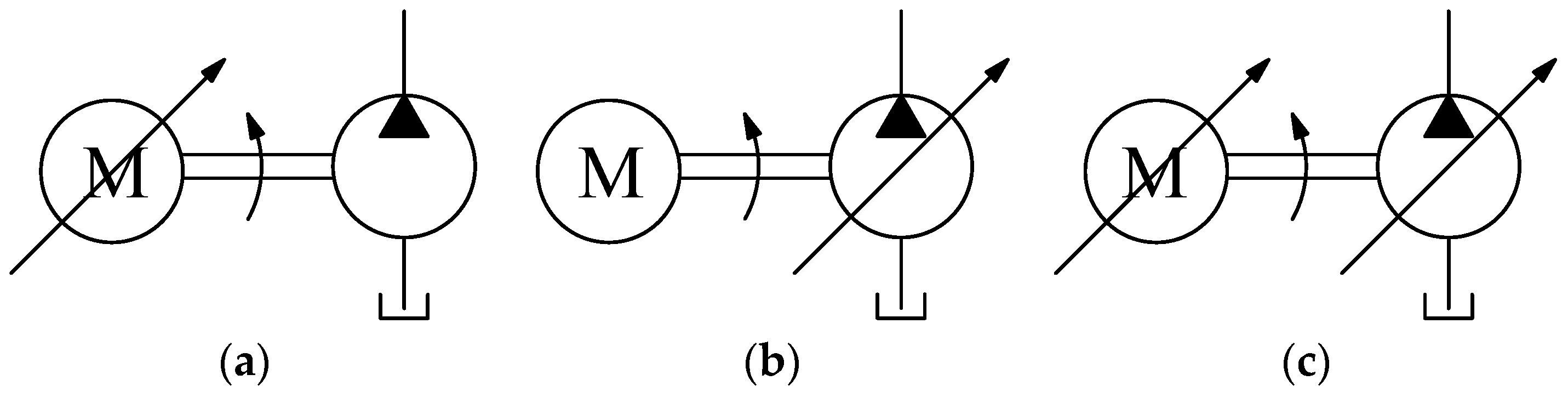
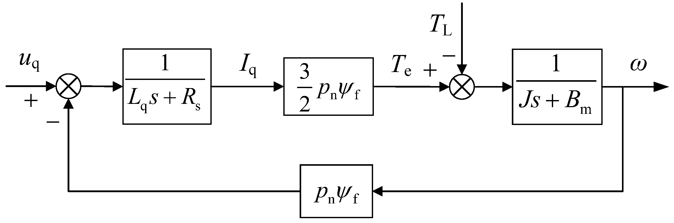
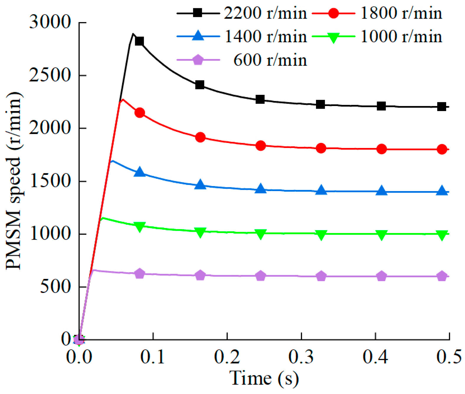
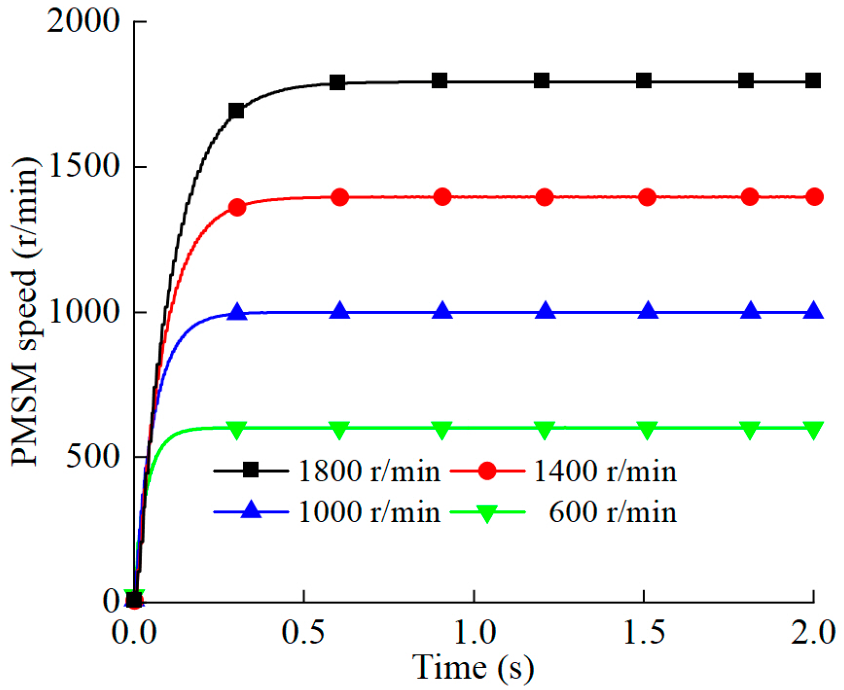
2.1. Dynamic Characteristics Analysis of the PMSM

The voltage equation of the PMSM is as follows:

$$\left\{\begin{array}{l}{u}_{\mathrm{d}}=R_{\mathrm{s}}{i}_{\mathrm{d}}-{\omega }_{\mathrm{e}}{L}_{\mathrm{q}}{i}_{\mathrm{q}}+L_{\mathrm{d}}\frac{d{i}_{\mathrm{d}}}{dt}\hfill \\ u_{\mathrm{q}}=R_{\mathrm{s}}{i}_{\mathrm{q}}+{\omega }_{\mathrm{e}}(L_{\mathrm{d}}{i}_{\mathrm{d}}+{\psi }_{\mathrm{f}})+L_{\mathrm{q}}\frac{d{i}_{\mathrm{q}}}{dt}\hfill \end{array}\right.$$

(1)

The electromagnetic torque equation of the PMSM is as follows:

$$T_{\mathrm{e}}=\frac{3}{2}{p}_{\mathrm{n}}{\psi }_{\mathrm{f}}{i}_{\mathrm{q}}$$

(2)

The mechanical motion equation of the PMSM is as follows:

$$T_{\mathrm{e}}=T_{\mathrm{L}}+B_{\mathrm{m}}\omega +J\frac{d\omega }{dt}$$

(3)

where u_d and u_q are the d-axis and q-axis voltage (V), ψ_f is the permanent magnet flux linkage (Wb), L_d and L_q are the d-axis and q-axis inductance (H), ω_e is the electrical angular velocity (rad/s), R_s is the stator phase resistance (Ω), T_e is the electromagnetic torque (N∙m), p_n is the number of poles of the PMSM, T_L is the load torque (N∙m), B_m is the damping coefficient (N/(m/s)), ω is the mechanical angular velocity (rad/s), and J is the rotor moment of inertia (kg∙m²).

Equations (1)–(3) are then transformed by Laplace transform as follows:

$$\left\{\begin{array}{l}{u}_{\mathrm{d}}=-p_{\mathrm{n}}\omega L_{\mathrm{q}}{I}_{\mathrm{q}}\\ u_{\mathrm{q}}=R_{\mathrm{s}}{I}_{\mathrm{q}}+L_{\mathrm{q}}{I}_{\mathrm{q}}s+p_{\mathrm{n}}\omega {\psi }_{\mathrm{f}}\\ T_{\mathrm{e}}=\frac{3}{2}{p}_{\mathrm{n}}{\psi }_{\mathrm{f}}{I}_{\mathrm{q}}\\ T_{\mathrm{e}}=T_{\mathrm{L}}+B_{\mathrm{m}}\omega +J\omega s\end{array}\right.$$

(4)

The PMSM control system block diagram is built according to Equation (4), as shown in Figure 2.

The speed of the PMSM is an important factor affecting the flow response of the VSVDPU. The response time and variation rule of the PMSM speed under different varying ranges and load torques were analyzed by simulation. The PMSM simulation parameters are shown in

Table 1. The PMSM simulation parameters.

Physical Parameter	Value of Number	Physical Unit
Nominal voltage	380	V
The d-axis inductance	0.84	mH
The q-axis inductance	2.72	mH
Stator phase resistance	0.1098	Ω
The number of poles of the PMSM	4	\
The permanent magnet flux linkage	0.185	Wb
The rotor moment of inertia	0.0375	kg∙m2
The damping coefficient	0.015	N/(m/s)
The gas density	1.29	kg/m3
The rotor radius	0.0345	m
The rotor axial length	0.34	m

.

In no-load conditions, we set the following step speed control commands for the PMSM: 600 r/min, 1000 r/min, 1400 r/min, 1800 r/min, and 2200 r/min. Figure 3 shows the PMSM response curves at different speeds.

According to Figure 3, the PMSM maintains a constant speed throughout the process of acceleration. The step response time of the PMSM at 600 r/min, 1000 r/min, 1400 r/min, 1800 r/min, and 2200 r/min is 15 ms, 24 ms, 34 ms, 44 ms, and 54 ms, respectively. Within the rated speed range, the response time of the PMSM under no-load conditions is approximately within 50 ms, and the longer the range of speed changes, the longer the response time.

Given a speed command of 1500 r/min for the PMSM, load torques of 20 N·m, 60 N·m, 100 N·m, and 140 N·m were subsequently applied. The response curves of the PMSM speed under loaded conditions are shown in Figure 4.

According to Figure 4, when the load torques are 20 N·m, 60 N·m, 100 N·m, and 140 N·m, respectively, the step response times for the PMSM at a speed of 1500 r/min are 42 ms, 58 ms, 95 ms, and 270 ms. As the load torque increases, the speed response of the PMSM slows down. In addition, the maximum response time of the PMSM speed across all operating conditions is in the order of several hundred milliseconds.

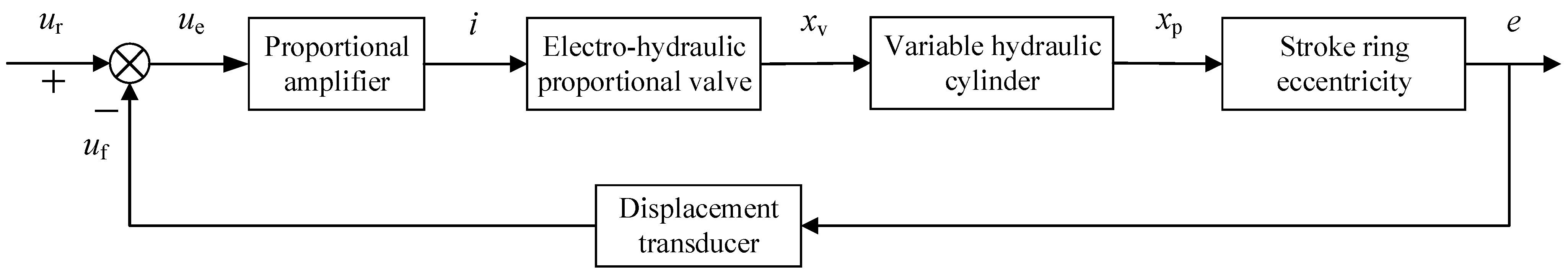
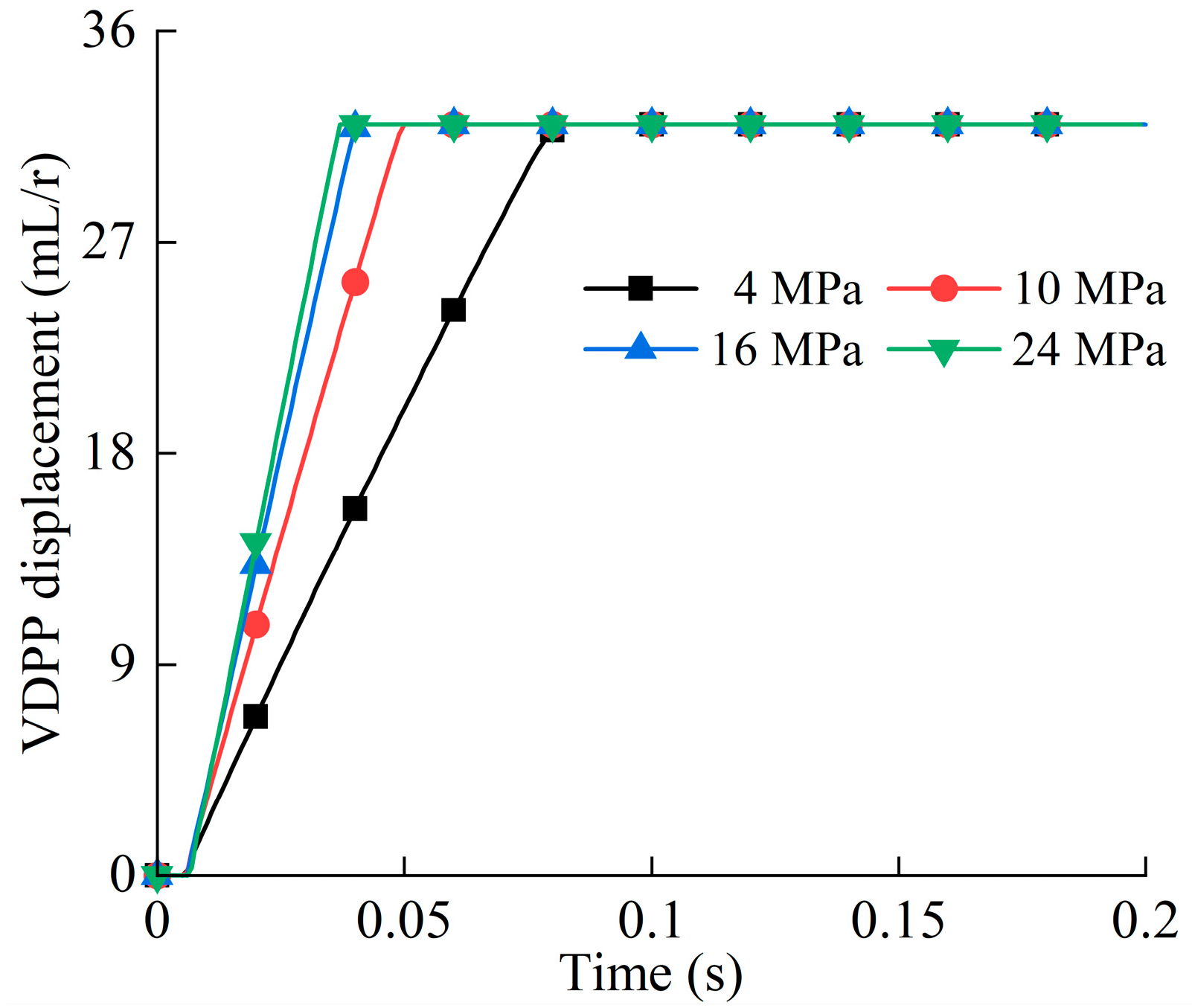
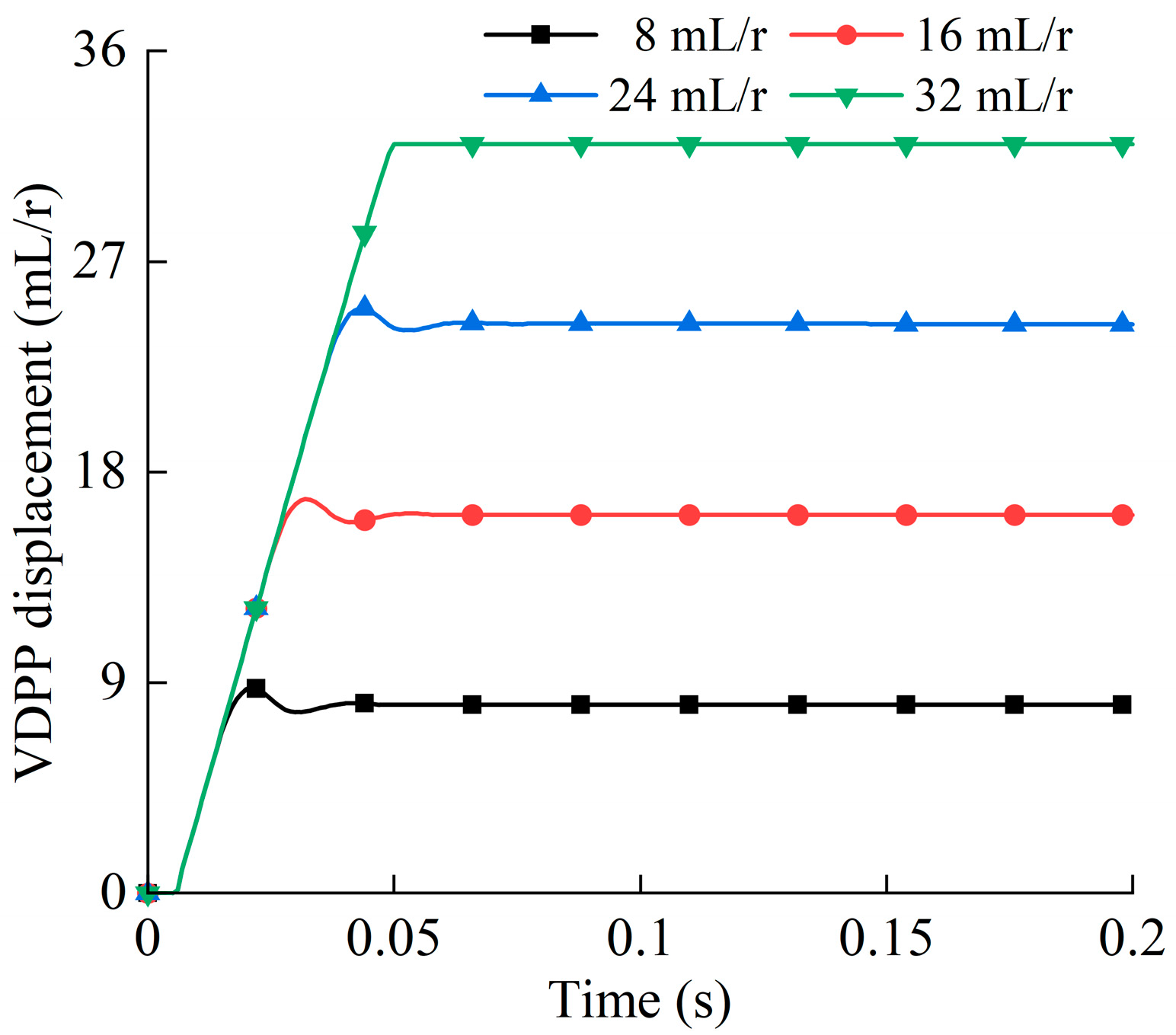
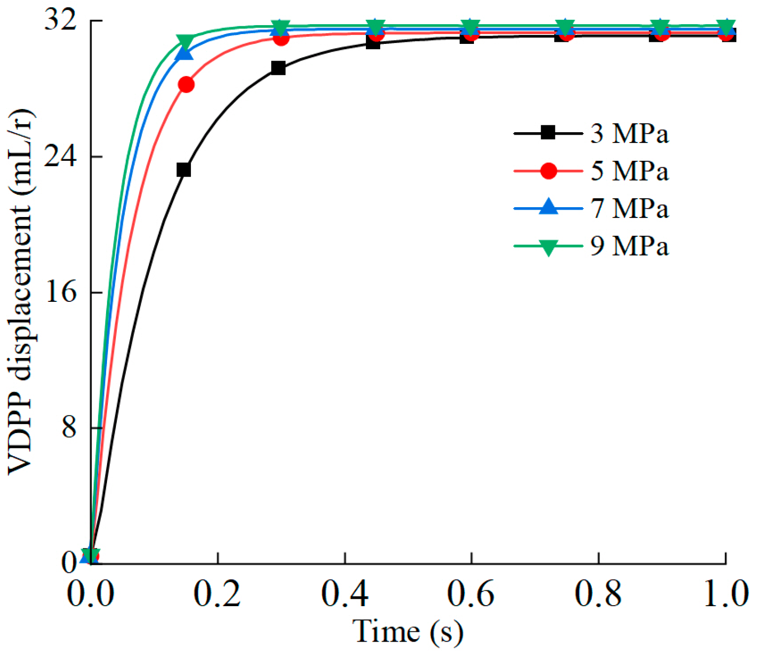
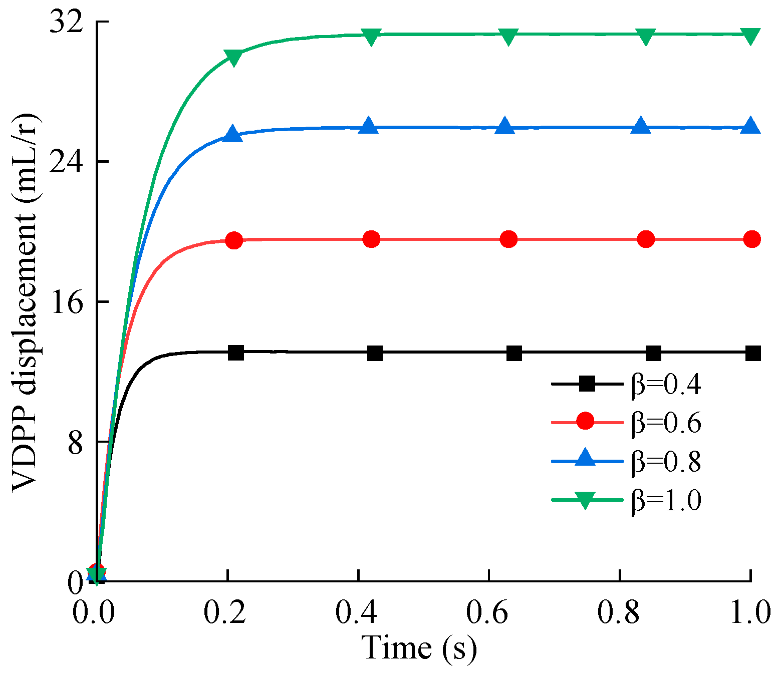
2.2. Dynamic Characteristics Analysis of the VDPP

This paper studied the VDPP, which is a radial piston pump. The displacement of the VDPP can be expressed as follows:

$$V=\frac{\pi d_{\mathrm{p}}^2}{2}Ze$$

(5)

where V is the displacement of the VDPP (m³/r), d_p is the plunger diameter (m), Z is the number of plungers, and e is the stroke ring eccentricity (m).

The variable mechanism of the VDPP is mainly composed of the proportional amplifier, controller, proportional valve, variable hydraulic cylinder, and displacement sensor. When the VDPP needs to change the displacement, it compares the target displacement signal with the feedback displacement signal. The deviation signal obtained is converted into a control signal for the proportional valve through the controller and the proportional amplifier. The proportional valve then outputs a controlled flow to drive the piston of the hydraulic cylinder until the stroke ring is moved to the target displacement position. The control block diagram of the variable mechanism is shown in Figure 5.

The deviation voltage of the variable mechanism and the spool displacement of the proportional valve can be approximately regarded as a proportional link, and its transfer function can be expressed as follows:

$$X_{\mathrm{v}}=K_{\mathrm{a}}{K}_{\mathrm{sv}}{U}_{\mathrm{e}}=K_{\mathrm{a}}{K}_{\mathrm{sv}}(U_{\mathrm{r}}-U_{\mathrm{f}})$$

(6)

where X_v is proportional valve spool displacement (m), K_a is the proportional amplifier gain (A/V), K_sv is proportional valve spool displacement gain (m/A), U_e is variable mechanism deviation voltage (V), U_r is the variable mechanism control input voltage (V), and U_f is the variable mechanism feedback voltage (V).

The VDPP variable mechanism is a valve-controlled hydraulic cylinder system, and its transfer function can be expressed as follows:

$$X_{\mathrm{p}}=\frac{\frac{K_{\mathrm{q}}}{A_{\mathrm{p}}}{X}_{\mathrm{v}}-\frac{K_{\mathrm{ce}}}{A_{\mathrm{p}}^2}(1+\frac{V_{\mathrm{t}}}{4{\beta }_{\mathrm{e}}{K}_{\mathrm{ce}}}s)F_{\mathrm{L}}}{(s+\frac{K_{\mathrm{ce}}K}{A_{\mathrm{p}}^2})(\frac{s^2}{{\omega }_{\mathrm{h}}^2}+\frac{2{\zeta }_{\mathrm{h}}}{{\omega }_{\mathrm{h}}}s+1)}$$

(7)

where X_p is the displacement of hydraulic cylinder piston (m), K_q is the proportional valve flow gain (m²/s), A_p is the effective area of the hydraulic cylinder piston (m²), K_ce is the flow pressure coefficient (m⁵/(N∙s)), V_t is the control chamber volume (m³), β_e is the oil bulk elastic modulus (N/m²), F_L is the load force outside the hydraulic cylinder (N), K is the load spring stiffness, ω_h is the hydraulic natural frequency (rad/s), and ζ_h is the hydraulic damping ratio.

The displacement of the hydraulic cylinder piston and the feedback voltage of the variable mechanism can be considered as proportional elements, and their transfer function can be expressed as follows:

$$U_{\mathrm{f}}=K_{\mathrm{t}}{K}_{\mathrm{e}}{X}_{\mathrm{p}}$$

(8)

where K_t is the displacement coefficient of the hydraulic cylinder piston and eccentricity of the stroke ring (m/m), and K_e is the variable mechanism feedback voltage and stroke ring eccentricity change coefficient (V/m).

By combining Equations (6)–(8), the block diagram of the VDPP variable mechanism control system can be obtained, as shown in Figure 6.

According to Figure 6, for the VDPP with fixed structural parameters, the dynamic and static characteristics of its variable process are disturbed by the load force of the variable hydraulic cylinder, and the magnitude of the load force is determined by the output pressure of the hydraulic pump. A simulation analysis was conducted to investigate the response time and variation patterns of the VDPP under different displacement ranges and system pressures. The VDPP simulation parameters are shown in

Table 2. The VDPP simulation parameters.

Physical Parameter	Value of Number	Physical Unit
The VDPP maximum displacement	32	mL/r
Plunger diameter	1.2 × 10−2	m
The number of plungers	9	\
The oil bulk elastic modulus	1.5 × 10−9	N/m2
The oil dynamic viscosity	2.61 × 10−2	Pa∙s
The variable mechanism input control voltage	±10	V
The effective area of the hydraulic cylinder piston	2.2 × 10−4	m2
The control chamber volume	1.5 × 10−5	m3

.

Given the maximum displacement command of the VDPP, the response times of displacement under different system pressures obtained by simulation are shown in Figure 7.

According to Figure 7, when the system pressure is 4 MPa, 10 MPa, 16 MPa, and 24 MPa, the response time from zero to maximum displacement is 80 ms, 50 ms, 40 ms, and 37 ms, respectively. The greater the system pressure, the faster the response time of displacement.

When the system pressure is maintained at 10 MPa, the response time curves of different displacement variations are shown in Figure 8.

According to Figure 8, when the system pressure is 10 MPa, the response times for the displacement varying from 0 mL/r to 8 mL/r, 16 mL/r, 24 mL/r, and 32 mL/r are 20 ms, 30 ms, 40 ms, and 50 ms, respectively. The larger the range of displacement change, the longer the response time. Additionally, it can be observed that when the system pressure remains unchanged, the speed of displacement change remains constant.

3. Energy Efficiency Characteristic Analysis of the VSVDPU

3.1. Energy Efficiency Characteristics Analysis of the PMSM

The power loss of the PMSM mainly includes mechanical loss, copper loss, iron loss, and power converter loss.

The mechanical loss of the PMSM can be expressed as follows:

$$P_{\mathrm{me}}=C_{\mathrm{b}}{D}_{\mathrm{m}}^3\omega +k_{\mathrm{m}}{C}_{\mathrm{f}}\pi \rho {\omega }^3{r}^{4}l$$

(9)

where P_me is the mechanical loss (W), C_b is the bearing load coefficient, D_m is the bearing diameter (m), k_m is the rotor surface roughness, C_f is the air friction coefficient, ρ is the air density (kg/m³), r is the rotor radius (m), and l is the rotor axial length (m).

The copper loss of the PMSM can be expressed as follows:

$$P_{\mathrm{Cu}}=m{I}^2{R}_{\mathrm{s}}$$

(10)

where P_cu is the winding copper loss (W), m is the number of phases of the PMSM, and I is the phase current (A).

The stator phase resistance is related to the winding temperature, which can be expressed as follows:

$$R_{\mathrm{s}}=R_{\mathrm{s}0}\frac{K+T}{K+T_0}$$

(11)

where R_s0 is the stator phase resistance at the initial moment, K is the resistance temperature coefficient (235 for copper wire and 225 for aluminum wire), T is the temperature at the current time, and T₀ is the temperature at the initial time.

The iron consumption of the PMSM can be expressed as follows:

$$P_{\mathrm{Fe}}=k_{\mathrm{h}}f{B}_{\mathrm{m}}^{\alpha }+k_{\mathrm{c}}{f}^2{B}_{\mathrm{m}}^2+k_{\mathrm{e}}{f}^{1.5}{B}_{\mathrm{m}}^{1.5}$$

(12)

where P_Fe is the stator iron loss (W), k_h is the hysteresis loss coefficient, k_c is the eddy current loss coefficient, k_e is the additional loss coefficient, f is the magnetic field frequency (Hz), B_m is the magnetic density amplitude (Wb/m²), and α is the Steinmetz coefficient, α = 2.

The power converter loss of the PMSM can be expressed as follows:

$$P_{\mathrm{dr}}=m{k}_{\mathrm{dr}}I$$

(13)

where P_dr is the power converter loss, and k_dr is the power converter loss coefficient.

The efficiency of the PMSM can be expressed as follows:

$${\eta }_{\mathrm{m}}=\frac{T_{\mathrm{e}}\omega }{T_{\mathrm{e}}\omega +P_{\mathrm{me}}+P_{\mathrm{Fe}}+P_{\mathrm{Cu}}+P_{\mathrm{dr}}}$$

(14)

The efficiency of the PMSM is related to the output torque and speed. The cloud diagram of the PMSM efficiency obtained by simulation is shown in Figure 9.

According to Figure 9, when the speed of the PMSM remains constant, its efficiency first increases and then decreases as the output torque rises. This is because as the output torque of the PMSM increases, the increment of the PMSM output power is greater than the increment of the loss power before reaching the optimal efficiency torque point, but then it becomes smaller. When the PMSM outputs a small torque, its efficiency decreases as the output speed increases. Conversely, when the PMSM outputs a large torque, its efficiency increases as the output speed increases. This is because at low torques, although the PMSM’s output speed increases, the output power remains relatively small, and the proportion of loss power is larger. At high torques, as the PMSM speed increases, both the output power and loss power increase, but the proportion of loss power decreases.

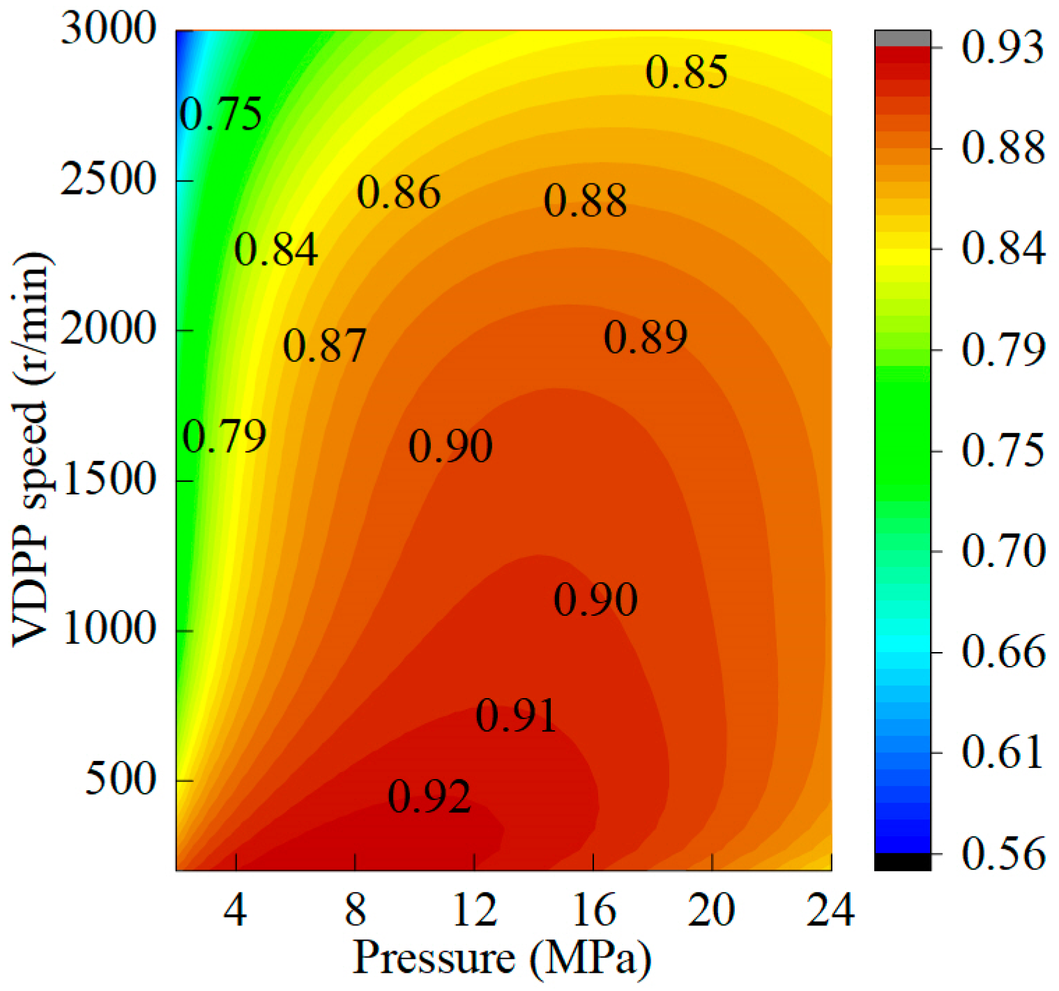
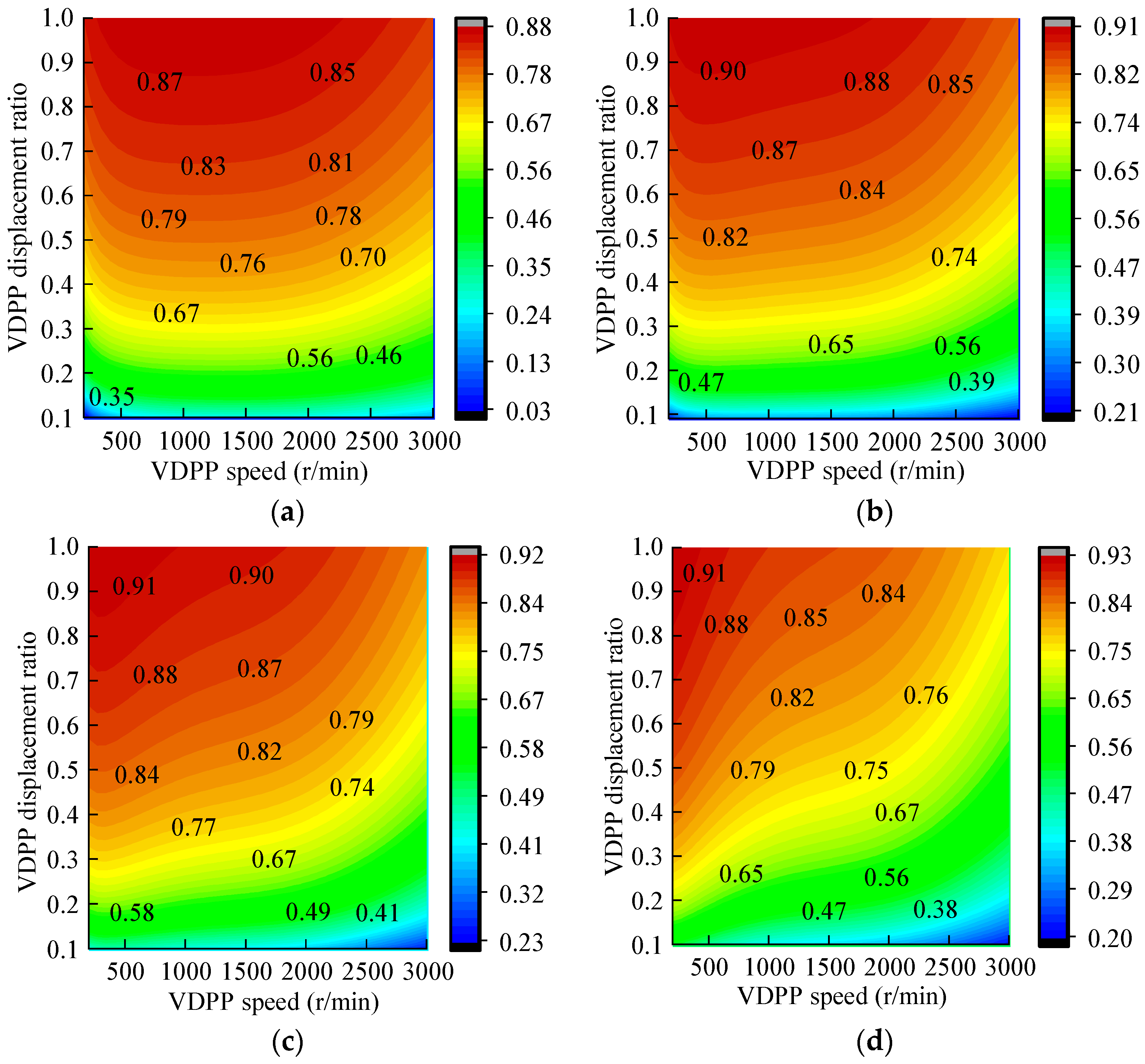
3.2. Energy Efficiency Characteristics Analysis of the VDPP

Ignoring the inlet pressure of the VDPP, the volumetric efficiency of the VDPP can be expressed as follows:

$${\eta }_{\mathrm{p}v}=1-\frac{60C_{\mathrm{s}}p}{\mu n\beta }$$

(15)

$$\beta =\frac{V}{V_0}$$

(16)

where η_pv is the volumetric efficiency, C_s is the laminar flow leakage coefficient, p is the outlet pressure (Pa), μ is the dynamic viscosity of oil (Pa∙s), n is the rotational speed (r/min), β is the displacement ratio, V₀ is the maximum displacement (m³/r), and V is the real-time displacement (m³/r).

The mechanical efficiency of the VDPP can be expressed as follows:

$${\eta }_{\mathrm{pm}}=\frac{1}{1+\frac{\mu n{C}_{\mathrm{v}}}{60p\beta }+\frac{C_{\mathrm{m}}}{\beta }+\frac{2\pi T_{\mathrm{s}}}{p{V}_0\beta }}$$

(17)

where η_pm is the mechanical efficiency of the VDPP, C_v is the laminar flow resistance coefficient, C_m is the mechanical resistance coefficient, and T_s is the torque loss constant (N∙m).

The total efficiency of the VDPP is the product of volumetric efficiency and mechanical efficiency, which can be expressed as follows:

$${\eta }_{\mathrm{p}}={\eta }_{\mathrm{pm}}{\eta }_{\mathrm{pv}}$$

(18)

The pressure differential between the inlet and outlet, displacement, and rotation speed all affect the VDPP total efficiency. The cloud diagram of the VDPP total efficiency under the maximum displacement obtained by simulation is shown in Figure 10.

According to Figure 10, when the system pressure is constant, the VDPP total efficiency first increases and then decreases as the speed increases. This is because the VDPP total efficiency is affected by low volumetric efficiency at a low-speed range and low mechanical efficiency at a high-speed range. When the VDPP speed is constant, the total efficiency of the VDPP increases first and then decreases with the pressure of the system, which is because the mechanical efficiency of the VDPP is small in the low-pressure region, and the volumetric efficiency of the VDPP is small in the high-pressure region. The VDPP total efficiency is the lowest at high speed and low pressure.

The VDPP total efficiency cloud diagram obtained by simulation under different system pressures is shown in Figure 11.

According to Figure 11, when system pressure and rotational speed are constant, the VDPP total efficiency gradually increases with the increase in displacement. When the system pressure and displacement are constant, the VDPP total efficiency first increases and then decreases with the increase in rotational speed. Under certain pressure conditions, the VDPP has different combinations of speed and displacement to meet certain flow requirements of the system. Finding the combination of speed and displacement to optimize the VDPP efficiency is very critical.

4. Optimized Matching Control of the VSVDPU Speed and Displacement

4.1. High Dynamic Optimization Matching

The VSVDPU can simultaneously adjust the speed and displacement to meet the flow requirements of the system. The relationship between the output flow q, speed n, and displacement V is as follows:

$$\frac{\mathrm{d}q}{\mathrm{d}t}=\frac{\mathrm{d}n}{\mathrm{d}t}V+n\frac{\mathrm{d}V}{\mathrm{d}t}$$

(19)

According to Equation (19), the speed of the VSVDPU flow response is related to the speed and displacement response and depends on the slower response. Therefore, when the system flow rate changes, the maximum value of the PMSM speed change time and the VDPP displacement change time should be as small as possible, to improve the response speed of the VSVDPU flow output.

The expression of the VDPP displacement change rate is as follows:

$$\alpha =\frac{dV}{dt}$$

(20)

where α is the velocity of displacement change (m³/r/s).

According to the analysis of the VDPP response characteristics in Section 2.2, the velocity of displacement change is mainly related to system pressure. When the system pressure is constant, the velocity of the VDPP displacement change can be regarded as a constant value.

The expression of the PMSM speed change rate is as follows:

$$\frac{dn}{dt}=\frac{1}{J}(T_{\max }-\frac{pV(t)}{2\pi })$$

(21)

where T_max is the maximum output torque of the PMSM (N∙m).

According to the PMSM response characteristics analysis in Section 2.1, the PMSM maintains the maximum electromagnetic torque output during the speed change, and the speed change depends on the maximum torque output capacity of the PMSM and the load size.

Assuming that the initial flow rate of the VSVDPU is q₁, the corresponding speed is n₁, and the displacement is V₁. If the target demand flow is q₂, the corresponding target speed is n₂, and the target displacement is V₂. The initial flow rate q₁ and the target flow rate q₂ can be expressed as follows:

$$\left\{\begin{array}{l}{q}_1=n_1{V}_1\\ q_2=n_2{V}_2\end{array}\right.$$

(22)

Assuming that the duration of the VDPP displacement change is t₁, the dynamic expression of the VDPP displacement is as follows:

$$V_2=V_1+\alpha t_1$$

(23)

Assuming that the duration of the PMSM speed change is t₂, the dynamic expression of the PMSM speed is as follows:

$$n_2-n_1=\frac{1}{J}{\displaystyle {\int }_0^{t_2}{T}_{\max }-\frac{pV(t)}{2\pi }}\mathrm{d}t$$

(24)

Integrating Equation (23) into Equation (24), when the duration of the PMSM speed change is less than or equal to the time of the VDPP displacement change, the dynamic expression of the PMSM speed can be further expressed as follows:

$$n_2-n_1=\frac{T_{\max }}{J}{t}_2-\frac{p}{2\pi J}(V_1{t}_2+\frac{1}{2}\alpha t_2^2)$$

(25)

When the duration of the PMSM speed change is greater than that of the VDPP displacement change, the dynamic expression of the PMSM speed can be further expressed as follows:

$$n_2-n_1=\frac{T_{\max }}{J}{t}_2-\frac{p}{2\pi J}(V_1{t}_1+\frac{1}{2}\alpha t_1^2+V_2{t}_2-V_2{t}_1)$$

(26)

When the system pressure is constant and the system flow rate changes from one steady-state value to another steady-state value, the t₁ and t₂ values corresponding to the combination of different speeds and displacements can be calculated by Equations (23), (25), and (26). In various combinations, the maximum values of t₁ and t₂ are the smallest, which is the scheme with the fastest dynamic response of the VSVDPU. This process is a single-objective optimization process, and the highly dynamic optimization model of the VSVDPU includes the following:

The objective function is as follows:

$$f_{\min }=\max \left[t_1(n,p,V),t_2(n,p,V)\right]$$

(27)

The constraint conditions are as follows:

$$s.t.\left\{\begin{array}{l}0\le V\le 32\times {10}^{-6}\\ 0\le n\le 3000\\ 0\le p\le 30\times {10}^6\end{array}\right.$$

(28)

In MATLAB R2020b software, the fmincon function was used to optimize the dynamic response of the VSVDPU flow output. The system was set to be in a constant pressure condition of 12 MPa, the initial flow rate of the system was 8 L/min, and the initial displacement of the VDPP was 8 mL/r. The optimal VSVDPU response displacement and response time when the output flow changed to different values were calculated by simulation and are as shown in Figure 12.

According to Figure 12, when the system pressure is constant, the combination of speed and displacement can always be found to make the VSVDPU dynamic response optimal under different flow variation ranges. When the system flow rate changes from 8 L/min to 64 L/min, the optimal response time of the VSVDPU can reach 35.92 ms.

4.2. High Efficiency Optimization Matching

According to the analysis of the VDPP and PMSM efficiencies in Section 3, the efficiency of the VDPP is mainly related to speed, pressure, and displacement. The efficiency of the VDPP can be expressed as follows:

$${\eta }_{\mathrm{p}}=f(n,p,V)$$

(29)

The efficiency of the PMSM is mainly related to speed and torque. The efficiency of the PMSM can be expressed as follows:

$${\eta }_{\mathrm{m}}=f(n,T)$$

(30)

The output torque of the PMSM is positively correlated with the displacement of the VDPP and system pressure. Therefore, the efficiency of the PMSM is also mainly related to rotational speed, pressure, and displacement. The efficiency of the PMSM can be further expressed as follows:

$${\eta }_{\mathrm{m}}=f(n,p,V)$$

(31)

The overall efficiency of the VSVDPU can be expressed as follows:

$$\eta ={\eta }_{\mathrm{p}}\cdot {\eta }_{\mathrm{m}}=f(n,p,V)$$

(32)

The efficiency of the VSVDPU is a nonlinear function related to rotational speed, displacement, and pressure. Under a certain system pressure, different combinations of rotational speed and displacement can meet the system specific flow requirements. Among these combinations, the one that maximizes the overall efficiency function value of the VSVDPU is considered the optimal efficiency solution for the VSVDPU. This process is also a single-objective optimization problem, and the optimization model for the VSVDPU efficiency includes the following:

The objective function is as follows:

$$g_{\max }=\eta (n,p,V)$$

(33)

The constraint conditions are the same as Equation (28).

In MATLAB software, the fmincon function was used to optimize the VSVDPU efficiency, and the system was set to be under a constant pressure of 12 MPa. The optimal combination of speed and displacement of the VSVDPU efficiency was simulated when the system flow rate varied in the range of 0–90 L/min and are as shown in Figure 13.

According to Figure 13, when the system operates at a pressure of 12 MPa, there always exists a combination of rotational speed and displacement that maximizes the overall efficiency of the VSVDPU at any given flow rate. As the system flow rate increases, the corresponding optimal efficiency first increases and then decreases, while the optimal displacement value increases accordingly. Within the flow rate range of 0–90 L/min, the overall optimal efficiency of the system is above 65%.

The optimal combination of the VSVDPU efficiency and displacement corresponding to different system flows under full pressure conditions was obtained by further simulation and are as shown in Figure 14.

According to Figure 14, it can be observed that when the system pressure is constant, as the system flow rate increases, the optimal efficiency of the VSVDPU first increases and then decreases, and the corresponding optimal displacement value of the VDPP also increases. When the system flow rate is constant and relatively low, the higher the system pressure, the lower the optimal efficiency of the VSVDPU, and the smaller the optimal displacement value of the VDPP. The optimal efficiency of the VSVDPU is the lowest under high-pressure and low-flow conditions.

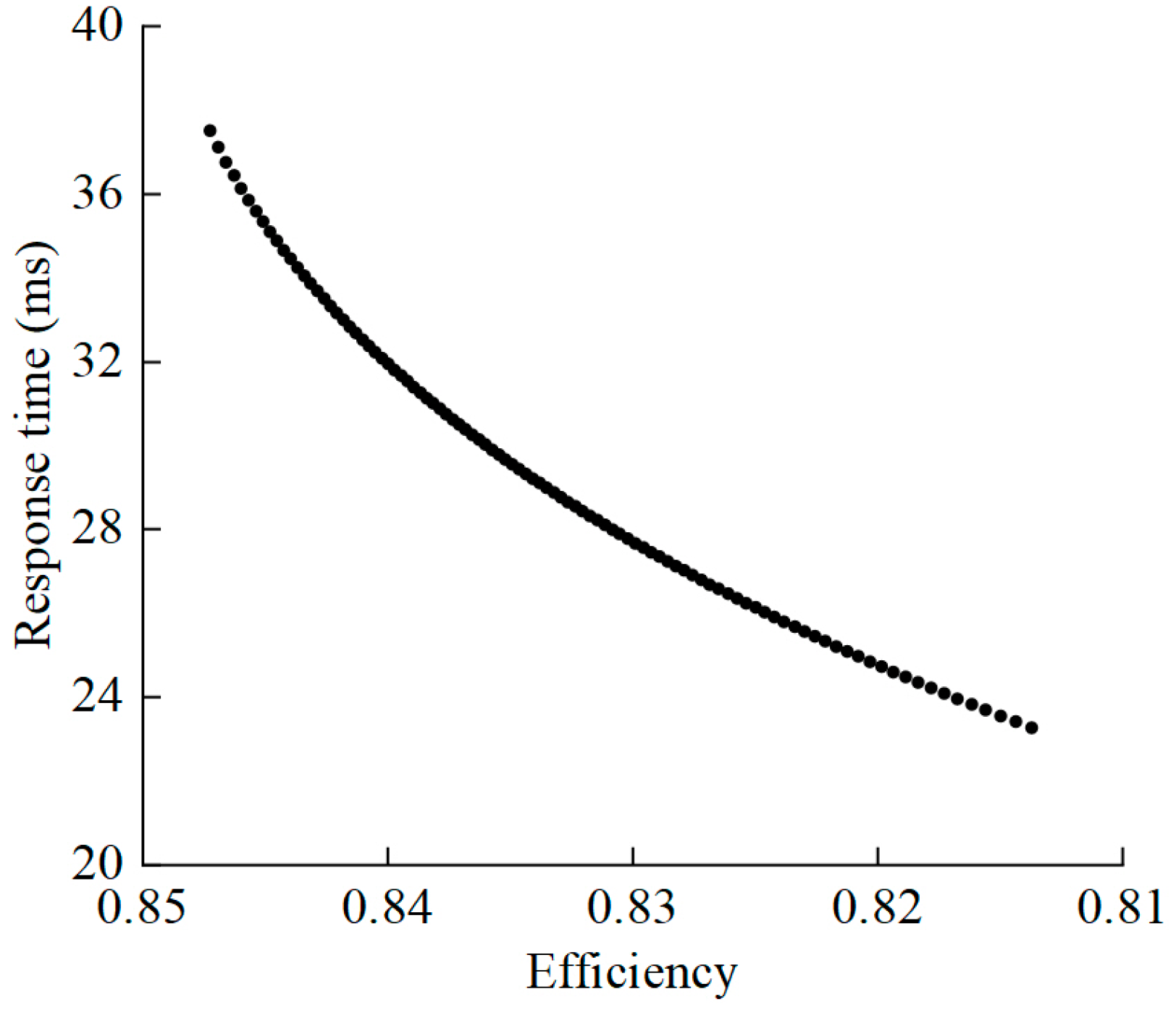
4.3. High Efficiency and Dynamic Multi-Objective Optimization Matching

The above section separately studied the optimal dynamic response and optimal efficiency of the VSVDPU. In this section, the multi-objective particle swarm optimization algorithm was adopted, taking into account the dynamic response performance of the VSVDPU flow output, to achieve efficient matching control of the PMSM and VDPP. The multi-objective optimization matching control method is shown in Figure 15.

Under constant pressure conditions, the objective functions for both the dynamic response and efficiency of the VSVDPU are related to rotational speed and displacement. When the system flow rate changes, the rotational speed of the PMSM can be indirectly calculated by knowing the displacement of the VDPP. Therefore, the displacement V of the VDPP was selected as the sole optimization variable. To balance dynamic response performance, the response time t for the flow output of the VSVDPU should be as small as possible, and the overall energy efficiency η of the VSVDPU during steady state should be as high as possible. Both the rotational speed of the PMSM and the displacement of the VDPP should be within their specified ranges during the optimization process. In summary, the efficient and high-dynamic multi-objective optimization matching control model for the VSVDPU is as follows:

$$\begin{array}{l}h=\min \left\{1-\eta (V),t(V)\right\}\\ s.t.\left\{\begin{array}{l}0\le V_2\le 32\times {10}^{-6}\\ 0\le \frac{q_2}{V_2}\le 3000\end{array}\right.\end{array}$$

(34)

Using MATLAB software for multi-objective particle swarm optimization, we set the population size of the particle swarm to 100 and the number of iterations to 10,000. Assuming the system operates under a constant pressure of 12 MPa, with an initial flow rate of 8 L/min and an initial displacement of the VDPP at 8 mL/r, when the system flow rate changes to 40 L/min, we would obtain the Pareto optimal solution set for the displacement of the VDPP through iterative calculations, as shown in Figure 16. The corresponding Pareto front is presented in Figure 17.

According to Figure 16 and Figure 17, the Pareto optimal solution set for the displacement of the VDPP is [23, 32]. The corresponding range of response time for the VSVDPU is [27.3, 37.5], and the range of overall energy efficiency for the VSVDPU is [0.81, 0.85]. The VSVDPU exhibits good dynamic response performance and high energy efficiency within the Pareto optimal solution set. Additionally, the Pareto front reveals a trade-off relationship between the dynamic response time and energy efficiency of the VSVDPU. Optimizing one performance metric often comes at the cost of reducing the other. In practical engineering applications, the optimal solution can be reasonably selected based on the priority of dynamic response and energy efficiency.

5. Experimental Study of the VSVDPU

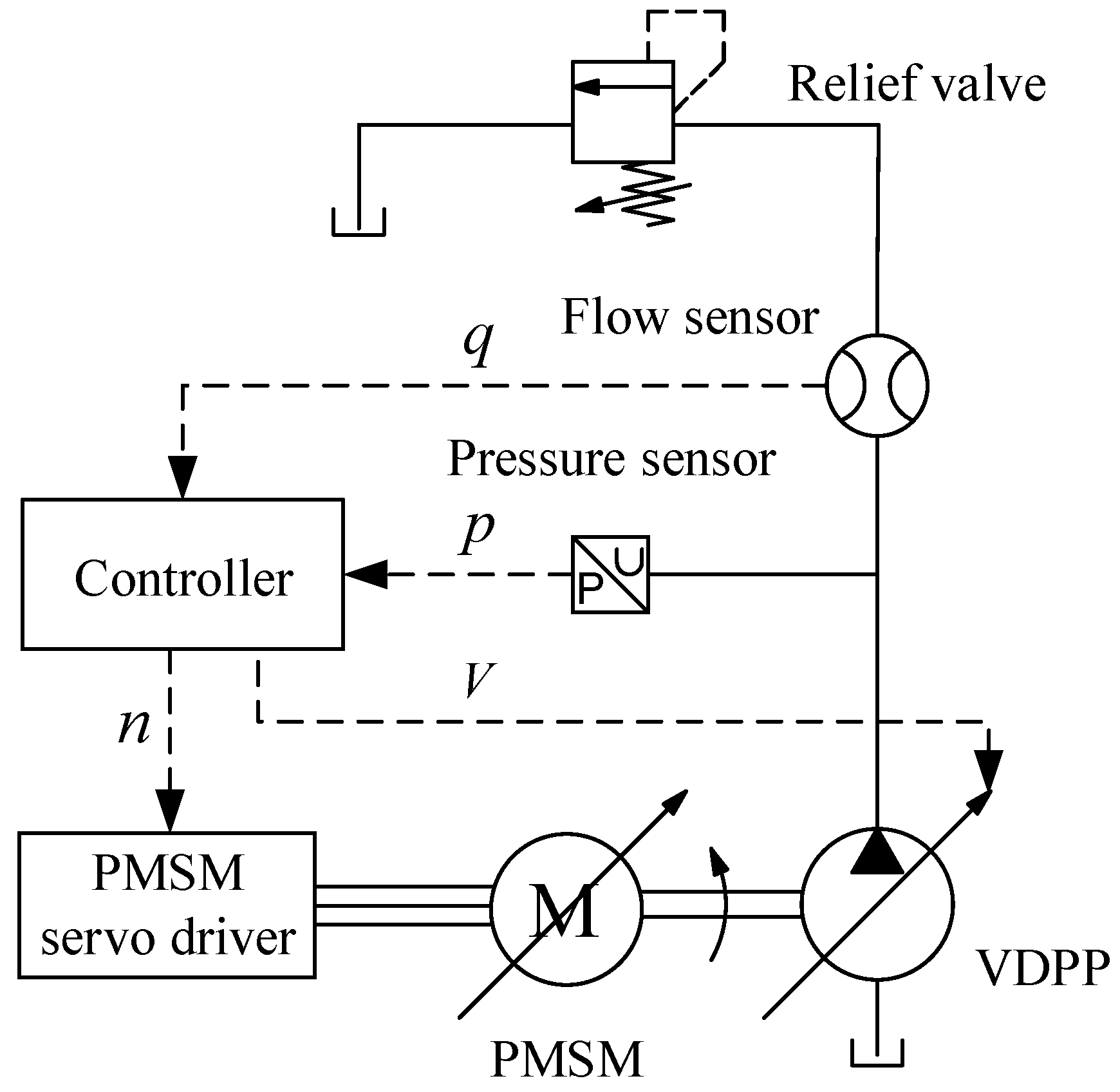
5.1. Construction of the VSVDPU Experimental Platform

The hydraulic principle of the VSVDPU experimental platform is illustrated in Figure 18. The experimental platform system primarily consists of a controller (MACS-I, Moog, New York, NY, USA), a driver (Hi308-441P6A05N7, Haitian, Ningbo, China), PMSM (HP11812-H182F, Haitian, Ningbo, China), VDPP (D952-HPR18A7SCP032, Moog, New York, NY, USA), relief valve, pressure sensors, and flow sensors. The relief valve simulates the load of the VSVDPU. The flow and pressure sensors collect the relevant data from the system and feedback to the controller. The multi-objective optimization matching algorithm is then imported into the controller and calculates the optimal displacement and speed. Finally, control signals are output to the PMSM and VDPP, enabling high-efficiency and high-dynamic control of the VSVDPU.

The overall structure of the VSVDPU experimental platform is shown in Figure 19.

The main parameters of the VSVDPU experimental platform are shown in

Table 3. The VSVDPU experimental platform parameters.

Physical Parameter	Value of Number	Physical Unit
The PMSM Rated speed	1800	r/min
The PMSM rated torque	220.5	N·m
The PMSM rated power	41.6	kW
The VDPP maximum displacement	32	mL/r
The VDPP maximum pressure	35	MPa
The VDPP maximum speed	1800	r/min
Pressure sensor range	0–40	MPa
Flow sensor range	2–75	L/min
Pressure regulation range of relief valve	0–35	MPa

.

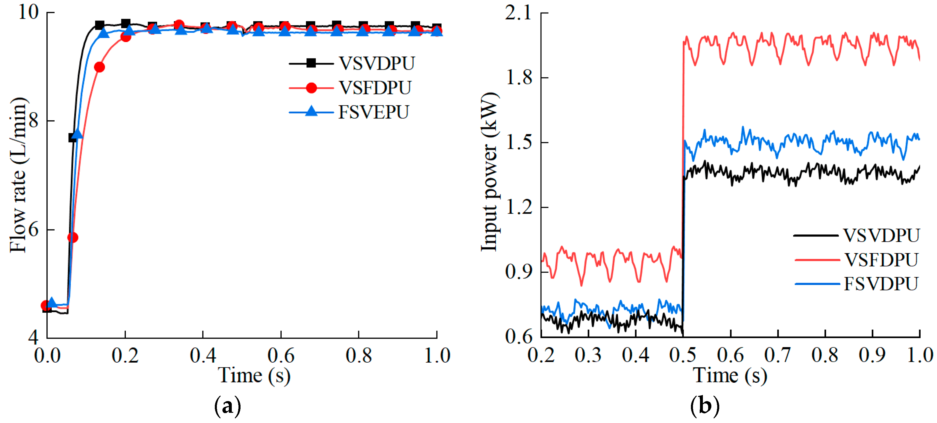
5.2. Analysis of the VSVDPU Experimental Results

In this section, the response characteristics of the PMSM and VDPP, the efficiency characteristics of the VSVDPU, and the high efficiency and dynamic matching control of the VSVDPU are studied experimentally.

The PMSM response test curves at different speeds when the VSVDPU is running in no-load conditions are shown in Figure 20.

According to Figure 20, the response times of the PMSM at 600 r/min, 1000 r/min, 1400 r/min, and 1800 r/min are 85 ms, 136 ms, 194 ms, and 257 ms, respectively. The response speeds of the PMSM are the same under different ranges.

When the PMSM speed is set to 500 r/min and the control command for the maximum displacement of the VDPP is given, the response curves of the VDPP displacement under load pressures of 3 MPa, 5 MPa, 7 MPa, and 9 MPa are shown in Figure 21. When the PMSM speed is set to 500 r/min and the load pressure is 5 MPa, the response curves of the VDPP displacement under displacement ratios of 0.4, 0.6, 0.8, and 1 are shown in Figure 22.

According to Figure 21, the response times for the maximum displacement of the VDPP under load pressures of 3 MPa, 5 MPa, 7 MPa, and 9 MPa are 247 ms, 153 ms, 117 ms, and 99 ms, respectively. The higher the load pressure on the VDPP, the faster the response time of its displacement. According to Figure 22, when the load pressure is 5 MPa, the response times of the VDPP displacement under control instructions of displacement ratios of 0.4, 0.6, 0.8, and 1 are 58 ms, 92 ms, 118 ms, and 153 ms, respectively. The larger the range of displacement changes, the longer the response time. When the load pressure is constant, the response speed for different displacement ranges is the same.

We then set the system load pressure to 4 MPa, and the speed of the PMSM was increased in increments of 200 r/min, while the VDPP displacement ratio was increased in increments of 0.1. The efficiency and speed–displacement curves of the VSVDPU are shown in Figure 23.

According to Figure 23, when the load pressure and speed are constant, the larger the VDPP displacement ratio, the higher the efficiency of the VSVDPU. When the system pressure and displacement are constant, the higher the PMSM speed, the higher the VSVDPU efficiency.

We then set the initial load pressure to 4 MPa and the flow rate to 5 L/min. At 0.05 s, a flow rate command of 10 L/min was given, and at 0.5 s, a load pressure command of 8 MPa was given. A comparison of the dynamic response and power input between the VSVDPU (under multi-objective optimization control), VSFDPU (with a displacement of 32 mL/r), and FSVDPU (at a speed of 1800 r/min) is shown in Figure 24.

According to Figure 24, when the system flow rate changes from 5 L/min to 10 L/min, the flow response times of the VSVDPU, VSFDPU, and FSVDPU are 38 ms, 57 ms, and 96 ms, respectively. Compared to the VSFDPU and FSVDPU, the response time of the VSVDPU is improved by 33.33% and 60.41%. When the load pressure is 4 MPa and the flow rate is 10 L/min, the average input powers of the VSVDPU, VSFDPU, and FSVDPU are 0.68 kW, 0.73 kW, and 0.96 kW. Compared to the VSFDPU and FSVDPU, the average input power of the VSVDPU is reduced by 6.85% and 29.17%. When the load pressure is 8 MPa and the flow rate is 10 L/min, the average input powers of the VSVDPU, VSFDPU, and FSVDPU are 1.39 kW, 1.51 kW, and 1.95 kW. Compared to the VSFDPU and FSVDPU, the average input power of the VSVDPU is reduced by 7.95% and 28.72%. This demonstrates that the multi-objective particle swarm optimization matching method proposed in this paper achieves high dynamic and efficient control of the speed and displacement of the VSVDPU.

6. Conclusions

This paper took the VSVDPU as the research subject and proposed an optimization matching control method based on the multi-objective particle swarm algorithm. This method took into account the dynamic response of the VSVDPU flow output, enabling efficient matching between the PMSM and VDPP. The main research findings are as follows:

The mathematical model of the dynamic response and efficiency of the PMSM and VDPP was established. It revealed the mechanism of how speed, displacement, and pressure parameters affect the dynamic response and efficiency of the VSVDPU. The optimization matching control method based on the multi-objective particle swarm optimization algorithm was proposed to achieve high efficiency and high dynamic matching between the speed and displacement of the VSVDPU. When the load pressure was 12 MPa and the flow rate varied from 8 L/min to 40 L/min, the optimal efficiency of the VSVDPU could reach 81~85% and the response time could be as short as 27.3~37.5 ms after applying the optimization matching control method based on the multi-objective particle swarm algorithm.

An experimental platform for matching and controlling the speed and displacement of the VSVDPU was constructed. When the system load pressure and rotational speed were constant, it was observed that the greater the displacement ratio of the VDPP, the higher the efficiency of the VSVDPU. Similarly, when the system pressure and displacement were constant, it was observed that the greater the rotational speed of the PMSM, the higher the efficiency of the VSVDPU. The experimental results tested the optimization matching control effect of the VSVDPU. When the load pressure was 4 MPa and the flow rate changed from 5 L/min to 10 L/min, compared to the VSFDPU and FSVDPU, the response time of the VSVDPU was improved by 33.33% and 60.41%, and the input power was reduced by 6.85% and 29.17%. When the load pressure was 8 MPa and the flow rate was 10 L/min, compared to the VSFDPU and FSVDPU, the system input power decreased by 7.95% and 28.72%, respectively. This verified that the optimization matching control method based on the multi-objective particle swarm optimization algorithm can achieve high-dynamic and high-efficiency matching control between the speed and displacement of the VSVDPU.

References

1. Yan, G.; Jin, Z.; Yang, M.; Yao, B. The thermal balance temperature field of the electro-hydraulic servo pump control system. Energies 2021, 14, 1364. [Google Scholar] [CrossRef]
2. Vacca, A. Energy efficiency and controllability of fluid power systems. Energies 2018, 11, 1169. [Google Scholar] [CrossRef]
3. Li, Z.; Shang, Y.; Jiao, Z.; Lin, Y.; Wu, S.; Li, X. Analysis of the dynamic performance of an electro-hydrostatic actuator and improvement methods. Chin. J. Aeronaut. 2018, 31, 2312–2320. [Google Scholar] [CrossRef]
4. Yu, B.; Wu, S.; Jiao, Z.; Shang, Y. Multi-Objective Optimization Design of an Electrohydrostatic Actuator Based on a Particle Swarm Optimization Algorithm and an Analytic Hierarchy Process. Energies 2018, 11, 2426. [Google Scholar] [CrossRef]
5. Yan, G.; Jin, Z.; Zhang, T.; Zhao, P. Position control study on pump-controlled servomotor for steam control valve. Processes 2021, 9, 221. [Google Scholar] [CrossRef]
6. Nguyen, M.T.; Dang, T.D.; Ahn, K.K. Application of Electro-Hydraulic Actuator System to Control Continuously Variable Transmission in Wind Energy Converter. Energies 2019, 12, 2499. [Google Scholar] [CrossRef]
7. Quan, Z.; Quan, L.; Zhang, J. Review of energy efficient direct pump controlled cylinder electro-hydraulic technology. Renew. Sustain. Energy Rev. 2014, 35, 336–346. [Google Scholar] [CrossRef]
8. Qu, S.; Fassbender, D.; Vacca, A.; Busquets, E. A high-efficient solution for electro-hydraulic actuators with energy regeneration capability. Energy 2021, 216, 119291. [Google Scholar] [CrossRef]
9. Zhang, X.; Huang, W.; Ge, L.; Quan, L. Research on response characteristics and energy efficiency of power unit used for electric driving mobile machine. IEEE Access 2019, 7, 125747–125753. [Google Scholar] [CrossRef]
10. Lovrec, D.; Tic, V.; Tasner, T. Simulation-aided determination of an efficiency field as a basis for maximum efficiency-controller design. Int. J. Simul. Model. 2015, 14, 669–682. [Google Scholar] [CrossRef]
11. Schmidt, L.; Hansen, K.V. Electro-Hydraulic Variable-Speed Drive Networks—Idea, Perspectives, and Energy Saving Potentials. Energies 2022, 15, 1228. [Google Scholar] [CrossRef]
12. Brecher, C.; Jasper, D.; Fey, M. Analysis of new, energy-efficient hydraulic unit for machine tools. Int. J. Precis. Eng. Manuf.-Green Technol. 2017, 4, 5–11. [Google Scholar] [CrossRef]
13. Huang, L.; Yu, T.; Jiao, Z.; Li, Y. Research on power matching and energy optimal control of active load-sensitive electro-hydrostatic actuator. IEEE Access 2020, 9, 51121–51133. [Google Scholar] [CrossRef]
14. Huang, J.; Yan, Z.; Quan, L.; Lan, Y.; Gao, Y. Characteristics of delivery pressure in the axial piston pump with combination of variable displacement and variable speed. Proc. Inst. Mech. Eng. Part I J. Syst. Control Eng. 2015, 229, 599–613. [Google Scholar] [CrossRef]
15. Han, X.; Zhang, P.; Minav, T.; Fu, Y.; Fu, J. A Modeling and Simulation Method for Preliminary Design of an Electro-Variable Displacement Pump. J. Vis. Exp. 2022, 184, e63593. [Google Scholar]
16. Cecchin, L.; Frey, J.; Gering, S.; Manderla, M.; Trachte, A.; Diehl, M. Nonlinear Model Predictive Control for Efficient Control of Variable Speed Variable Displacement Pumps. IFAC-PapersOnLine 2023, 56, 331–336. [Google Scholar] [CrossRef]
17. Willkomm, J.; Wahler, M.; Weber, J. Process-adapted control to maximize dynamics of speed-and displacement-variable pumps. In Proceedings of the ASME/BATH 2014 Symposium on Fluid Power and Motion Control, Bath, UK, 10–12 September 2014; p. V001T01A015. [Google Scholar]
18. Jin, R.; Huang, H.; Li, L.; Zuo, H.; Gan, L.; GE, S.; Liu, Z. Artificial Intelligence Enabled Energy-Saving Drive Unit with Speed and Displacement Variable Pumps for Electro-Hydraulic Systems. IEEE Trans. Autom. Sci. Eng. 2023, 99, 1–12. [Google Scholar] [CrossRef]
19. Zhang, Y.; Fu, Y.; Zhou, W. Optimal control for EHA-VPVM system based on feedback linearization theory. In Proceedings of the 2010 11th International Conference on Control Automation Robotics & Vision, Singapore, 7–10 December 2010; pp. 744–749. [Google Scholar]
20. Malrait, F.; Ejjabraoui, K. Power conversion optimization for hydraulic systems controlled by variable speed drives. J. Process Control 2019, 74, 133–146. [Google Scholar] [CrossRef]
21. Kim, H.; Yoo, S.; Cho, S.; Yi, K. Hybrid control algorithm for fuel consumption of a compound hybrid excavator. Automation in Construction 2016, 68, 1–10. [Google Scholar] [CrossRef]
22. Assaf, H.; Sarode, S.; Vacca, A.; Sudhoff, S.D. Electric machine sizing consideration for ePumps in mobile hydraulics. Energy Sci. Eng. 2024, 12, 793–809. [Google Scholar] [CrossRef]
23. Brecher, C.; Fey, M.; Brockmann, B.; Chavan, P. Multivariable control of active vibration compensation modules of a portal milling machine. J. Vib. Control 2018, 24, 3–17. [Google Scholar] [CrossRef]
24. Huang, H.; Jin, R.; Li, L.; Liu, Z. Improving the energy efficiency of a hydraulic press via variable-speed variable-displacement pump unit. J. Dyn. Syst. Meas. Control 2018, 140, 111006. [Google Scholar] [CrossRef]
25. Yan, Z.; Ge, L.; Quan, L. Energy-Efficient Electro-Hydraulic Power Source Driven by Variable-Speed Motor. Energies 2022, 15, 4804. [Google Scholar] [CrossRef]
Figure 1. Three combination schemes of the EHPU: (a) VSFDPU; (b) FSVDPU; (c) VSVDPU.
Energies 17 03322 g001
Figure 2. The PMSM control system block diagram.
Energies 17 03322 g002
Figure 3. Response curves of the PMSM at different speeds in no-load conditions.
Energies 17 03322 g003
Figure 4. Speed response curves of the PMSM under different loaded conditions.
Energies 17 03322 g004
Figure 5. Control block diagram of the VDPP variable mechanism.
Energies 17 03322 g005
Figure 6. The VDPP variable mechanism control system block diagram.
Energies 17 03322 g006
Figure 7. Response curves of the VDPP displacement under different system pressures.
Energies 17 03322 g007
Figure 8. Response curves of the VDPP with different displacements under constant pressure.
Energies 17 03322 g008
Figure 9. Cloud diagram of the relationship between the PMSM efficiency and speed torque.
Energies 17 03322 g009
Figure 10. Relationship between the inlet and outlet pressure differences, speed, and the VDPP total efficiency.
Energies 17 03322 g010
Figure 11. Relationship among the VDPP total efficiency, speed, and displacement under different pressures: (a) 24 MPa; (b) 18 MPa; (c) 12 MPa; (d) 6 MPa.
Energies 17 03322 g011
Figure 12. Optimal response results under different flow variation ranges.
Energies 17 03322 g012
Figure 13. Optimal efficiency results under different flows at 12 MPa pressure.
Energies 17 03322 g013
Figure 14. Optimal displacement and efficiency of the VSVDPU under all operating conditions: (a) optimal displacement; (b) optimal efficiency.
Energies 17 03322 g014
Figure 15. Multi-target optimization matching control method.
Energies 17 03322 g015
Figure 16. Pareto optimal solution of multi-objective optimization.
Energies 17 03322 g016
Figure 17. Pareto frontier of multi-objective optimization.
Energies 17 03322 g017
Figure 18. The hydraulic principle of the VSVDPU experimental platform.
Energies 17 03322 g018
Figure 19. The VSVDPU experimental platform.
Energies 17 03322 g019
Figure 20. Response test curves of the PMSM at different speeds.
Energies 17 03322 g020
Figure 21. Displacement response curves under different load pressures.
Energies 17 03322 g021
Figure 22. Displacement response curves under different displacement variation ranges.
Energies 17 03322 g022
Figure 23. Efficiency cloud map of the VSVDPU under different speeds and displacements.
Energies 17 03322 g023
Figure 24. Comparison of dynamic response and energy efficiency among three power units: (a) flow rate response; (b) input power.
Energies 17 03322 g024