Article

Addressing Data Scarcity in Solar Energy Prediction with Machine Learning and Augmentation Techniques

by
Aleksandr Gevorgian
1,
Giovanni Pernigotto
1,2,* and
Andrea Gasparella
1
1
Faculty of Engineering, Free University of Bozen-Bolzano, 39100 Bolzano, Italy
2
Competence Centre for Mountain Innovation Ecosystems, Free University of Bozen-Bolzano, 39100 Bolzano, Italy
*
Author to whom correspondence should be addressed.
Energies 2024, 17(14), 3365; https://doi.org/10.3390/en17143365
Submission received: 30 May 2024 / Revised: 3 July 2024 / Accepted: 5 July 2024 / Published: 9 July 2024
(This article belongs to the Topic Solar Forecasting and Smart Photovoltaic Systems)

Abstract

:
The accurate prediction of global horizontal irradiance (GHI) is crucial for optimizing solar power generation systems, particularly in mountainous areas with complex topography and unique microclimates. These regions face significant challenges due to limited reliable data and the dynamic nature of local weather conditions, which complicate accurate GHI measurement. The scarcity of precise data impedes the development of reliable solar energy prediction models, impacting both economic and environmental outcomes. To address these data scarcity challenges in solar energy prediction, this paper focuses on various locations in Europe and Asia Minor, predominantly in mountainous regions. Advanced machine learning techniques, including random forest (RF) and extreme gradient boosting (XGBoost) regressors, are employed to effectively predict GHI. Additionally, optimizing training data distribution based on cloud opacity values and integrating synthetic data significantly enhance predictive accuracy, with R2 scores ranging from 0.91 to 0.97 across multiple locations. Furthermore, substantial reductions in root mean square error (RMSE), mean absolute error (MAE), and mean bias error (MBE) underscore the improved reliability of the predictions. Future research should refine synthetic data generation, optimize additional meteorological and environmental parameter integration, extend methodology to new regions, and test for predicting global tilted irradiance (GTI). The studies should expand training data considerations beyond cloud opacity, incorporating sky cover and sunshine duration to enhance prediction accuracy and reliability.

1. Introduction

Solar energy stands as a pivotal pillar of sustainable development, as highlighted by the International Energy Agency (IEA) in 2020 [1]. Solar irradiance predictions, especially global horizontal irradiance (GHI), are crucial for efficiently harnessing this renewable resource [2]. Accurate GHI prediction is essential for optimizing solar energy system performance, planning, and maintenance. It enables the precise estimation of energy yields, which is crucial for cost-effective system design and efficient grid integration. These capabilities are fundamental for increasing the adoption and reliability of solar energy systems, supporting their sustainable growth and impact.
However, obtaining precise measurements of GHI pose significant challenges due to various factors. GHI, representing the total solar radiation received per unit area on a horizontal surface, is heavily influenced by dynamic atmospheric conditions like clouds, aerosols, and water vapor. The geographical location plays a crucial role, impacting measurement accuracy due to varying angles of incidence and atmospheric attenuation. In mountainous regions, these challenges are even more pronounced. Variable topography, microclimates, and inconsistent weather patterns create additional obstacles for accurate GHI prediction. The shadows from mountains and rapid weather changes can significantly affect solar irradiance, making predictions more complex and less reliable.
Instrumentation limitations, such as sensor calibration and maintenance issues, further complicate the task. Long-term data collection is necessary to accurately capture seasonal and diurnal variations, adding another layer of complexity. Additionally, free satellite GHI data providers often do not offer the high spatial and temporal resolution necessary for accurate measurements in complex environment such as mountains and urban regions. These challenges underscore the difficulty in achieving precise GHI measurements, essential for reliable solar energy assessments and applications [3,4].
As a consequence, building a comprehensive and precise dataset of GHI measurements demands substantial resources. Obtaining such data requires not only high-quality, specialized equipment but also significant financial investment [5]. Ensuring the accuracy of these readings is crucial, necessitating the regular maintenance of the equipment to keep precision and reliability over time. Additionally, numerous scientific studies emphasize the importance of investing in equipment and the challenges associated with acquiring GHI data, further highlighting the critical need for precise measurement [6,7]. The accuracy of GHI measurements is pivotal, as any errors can have a cascading effect on the entire solar energy prediction process. The far-reaching consequences of such inaccuracies can impact both the economic and environmental aspects [8,9]. Inaccurate GHI data can lead to flawed solar energy forecasts, resulting in potential financial losses and the suboptimal utilization of solar resources, thereby affecting the overall efficiency and sustainability of solar energy systems. Thus, the precision of GHI measurements is integral to the advancement and reliability of solar energy technologies.
In recent years, machine learning (ML) techniques have gained significant traction in solar energy prediction, promising technological advancements [2,10]. ML methods utilize sophisticated algorithms to analyze extensive datasets on solar energy production, enabling the accurate estimation of solar radiation [11,12]. These algorithms excel in identifying complex patterns, enhancing the efficiency and reliability of solar energy forecasts [13]. Moreover, artificial intelligence (AI) techniques like artificial neural networks (ANNs), genetic algorithms, and ML have demonstrated superior performance over traditional methods [14,15,16,17,18]. Hybrid models such as those combining long short-term memory networks (LSTM) and convolutional neural networks (CNNs) [19], as well as ensemble methods utilizing multiple ML algorithms [20], further exemplify the advances in solar radiation forecasting.
However, the following critical challenge arises: the effectiveness of these ML algorithms is heavily reliant on the quantity and quality of the training dataset. Frequently, the scarcity of accessible data becomes a bottleneck, hindering the creation of precise solar energy prediction models [21,22]. Therefore, there is a pressing demand for cost-effective approaches capable of efficiently obtaining and utilizing GHI data to enhance the accuracy of solar energy prediction models. The quality of the training dataset plays a crucial role in determining the effectiveness of ML algorithms [22]. High-quality data are essential for artificial intelligence (AI) systems to deliver meaningful results, as they possess several key attributes, such as accuracy, completeness, and reliability. Inaccurate or incomplete data can mislead AI models and produce unreliable outputs, leading to incorrect conclusions and reduced model performance [23]. Data acquisition costs, privacy concerns, and the presence of irrelevant or noisy data are some of the challenges associated with increasing the quantity of data [24,25]. Moreover, the relationship between data quality and data quantity is task-specific and requires human engineering [26].
In the context of solar energy prediction, the quality of the data is particularly important, as it directly impacts the accuracy and reliability of the predictions. Gathering high-quality GHI data is essential for developing accurate solar energy prediction models, which in turn can help optimize the performance of solar power systems and improve their integration into the grid [27]. Considering the challenge of limited accessible data for solar energy prediction models, our study introduces a methodology aimed at improving the accuracy of GHI prediction, even with constrained datasets. We leverage machine learning by employing the random forest (RF) algorithm [28] in conjunction with the extreme gradient boosting (XGBoost) regressor [29]. This integration enhances the accuracy of decision trees within the RF ensemble model, aiming to improve prediction accuracy. We focus on optimizing the distribution of training data based on cloud opacity values, a significant factor in GHI estimations [30,31]. Additionally, we generate synthetic data points, which are then augmented using techniques such as flipping, rotating, scaling, and the introduction of random noise [32]. This augmentation strategy diversifies the dataset, aiming to improve the model’s robustness against environmental variations. By enriching dataset variability through synthetic augmentation, our approach seeks to enhance model performance and resilience. In this way, this research addresses data scarcity challenges in solar energy prediction across various locations in Europe and Asia Minor, encompassing diverse geographical features such as mountainous terrain, alpine regions, urban areas, and plain zones.

2. Materials and Methods

2.1. Data Collection

In this study, global horizontal irradiance (GHI) across various locations was analyzed using data from 2019 and 2021. This study strategically chose regions across Europe and Asia, encompassing diverse topographies such as the Alps and other mountainous areas, known for their unique microclimates. Ground-based GHI measurements were randomly selected from various mountain plateaus to ensure an unbiased analysis. Random sites from non-mountainous environments were also included for comparative analysis, evaluating the model’s performance across different terrains. These regions, serving as the training and testing sites for the GHI prediction model, are illustrated in Figure 1, with details summarized in Table 1, including geographical coordinates and reference weather stations where GHI was measured.
Data collection relied on the following two primary sources: Visual Crossing provided GHI data [34], and Solcast supplied the historical actual meteorological year (AMY) weather and atmospheric data used as independent variables [35]. The preference for AMY data over typical meteorological year (TMY) data arises from the more accurate representation of specific years’ meteorological conditions, capturing variability and trends essential for precise solar irradiance prediction amidst dynamic weather and climate change impacts [36,37].
The methodology required the use of data from two different years: specifically, 1% of the 2019 data was used for model training, while the entire dataset from 2021 was used for testing to ensure robustness against overfitting. TMY data, based on historical records, cannot fulfill this requirement.
Visual Crossing provided comprehensive site-specific GHI data collected at hourly intervals, ensuring high temporal resolution, and covering various geographic locations within the specified regions. This spatial coverage facilitated capturing diverse climatic conditions and microclimates across Europe and Asia Minor. Solcast’s data included key environmental, solar geometry, and temporal variables as indicated in Table 2, crucial for the model’s training and testing. These data encompassed the following seven pivotal meteorological and atmospheric quantities: air temperature, cloud opacity, precipitable water, relative humidity, surface pressure, wind direction, and wind speed. Additionally, solar geometry variables and temporal inputs such as azimuth, zenith angles, month, day, and hour were incorporated at hourly intervals to align with GHI prediction needs. The predictors’ high spatial resolution of approximately 1 km2 [35] facilitates a detailed analysis of meteorological conditions, capturing the nuances of local weather patterns and their impacts on solar irradiance. Temporal data from Solcast, also provided at hourly intervals, ensured consistency with the GHI data from Visual Crossing. Solcast provided a detailed methodology for data preprocessing and quality control as outlined in their documentation [31].
Integrating these datasets created a robust ML framework for accurate GHI predictions in challenging environments. This approach addresses data scarcity and variability, ensuring reliable solar energy prediction and optimization.
As specified before, we utilized a random forest (RF) regressor [28] in conjunction with an extreme gradient boosting (XGBoost) regressor [29] trained on the 2019 dataset to predict the global horizontal irradiance (GHI) and test the model’s accuracy on a new unseen 2021 dataset. We intentionally used a different year for both training and testing the model to prevent overfitting.

2.2. Random Forest Regressor

RF regressor is an ML model that predicts continuous outcomes by combining predictions from multiple decision trees (DTs) [28]. It is known for its robustness and accuracy, achieved by training each tree on random subsets of data. The final prediction is obtained by averaging the predictions of all trees in the forest. The construction and operation of RF involve several key steps:
  • Bootstrapped dataset: Before constructing each DT in RF, a bootstrapped dataset is formed by randomly selecting data points from the original training dataset, with replacement. This ensures that each data point from the original training dataset has an equal chance of being chosen. As a result, some data points may be selected multiple times, while others may not be selected at all. Each DT in RF is trained on its own bootstrapped dataset, enabling them to learn from slightly different perspectives of the original training dataset. This diversity among the trees enhances the overall robustness and effectiveness of the RF model.
  • The root node: The root node symbolizes the starting point of the decision tree. It encompasses the entire bootstrapped dataset, serving as the foundation for the subsequent partitioning process. At this initial stage, the algorithm evaluates various predictors to determine the optimal split that divides the dataset into more homogeneous subsets. This decision sets the course for further branching, shaping the structure of the tree as it progresses. Ultimately, the root node plays a crucial role in guiding the recursive partitioning process, leading to the formation of internal nodes and leaf nodes that collectively constitute the DT model.
  • The internal node: Each internal node represents a pivotal point in the decision tree’s path. At these nodes, the bootstrapped dataset undergoes division into subsets based on true/false conditions, determined by predictors like zenith angle, dew point temperature, cloud opacity, etc. Utilizing the mean squared error (MSE), the algorithm selects the optimal split at each node. This process aims to minimize the variance within each subset, thus facilitating the creation of groups with closely aligned GHI values. The recursive splitting continues from the root node down the tree until reaching the leaf nodes, guiding the tree’s evolution toward more refined predictions. The mean squared error (MSE) is calculated using the following formula:
    M S E = 1 n i = 1 n = ( y i ŷ i ) 2
    Here, n represents the number of samples, y i denotes the actual GHI values, and ŷ i signifies the predicted GHI values for each sample.
  • Stopping criteria: Stopping criteria prevent the algorithm from excessively splitting the data, ensuring the model does not become overly complex or specific to the training data. The algorithm typically stops when each group of data at a node becomes quite small, either containing just one sample or having samples with identical GHI values. This ensures better generalization to new data.
  • The leaf node: A leaf node represents the endpoint of a branch in the tree. It signifies a terminal point where no further splits occur. Each leaf node contains the predicted GHI value for the subset of data that has traversed through the tree and arrived at that specific node. This prediction is based on a particular combination of inputs (e.g., air temperature, cloud opacity) and is calculated as the average GHI value derived from the actual GHI values of the samples in that subset. Leaf nodes serve as the final predictions made by the decision tree model.
  • Ensemble aggregation: Each decision tree within the RF makes a prediction at its leaf nodes based on the data it was trained on. The RF model then collects these predictions from all its trees and typically calculates the average to determine the final prediction. This means the RF’s prediction is essentially an average of the predictions from each decision tree, each contributing based on the subset of the data from which it has learned. This ensemble method enhances the prediction’s accuracy and stability, as it combines the strengths of multiple trees, rather than depending on just one.
  • Prediction on unseen data: When new predictors are introduced, the tree uses the splits it learned during training to navigate the new data point down the tree. The new data follow splits introduced during model training, and any deviation in predictor values leads to a corresponding adjustment in the predicted target value. Since the model has been trained on a variety of data samples, it can handle different scales and distributions in the predictors space. The final prediction for the unseen target is derived by averaging the predictions from all the trees, which compensates for any individual tree’s errors and leads to a more accurate and stable prediction.
The process of splitting the bootstrapped dataset in the model, from the root node through the internal nodes to the leaf nodes, is illustrated in Figure 2. This diagram captures a single DT within the RF, showcasing how the algorithm recursively partitions the data based on feature values to build a predictive model. Each split represents a decision rule applied to a subset of the data, ultimately leading to the leaf nodes, which provide the final predictions. This visualization helps to understand the hierarchical structure and decision-making process within RF.

2.3. Extreme Gradient Boosting Regressor

The next step in the analysis was to employ extreme gradient boosting (XGBoost) [29] in the RF to enhance the regression model’s performance. XGBoost applies a boosting technique to each decision tree within the RF ensemble, iteratively improving the regression predictions based on the residuals from previous trees. Mathematically, the boosting process can be explained as follows:
  • Initialization: Given a training dataset x i ,   y i i = 1 N , where ( x i ) represents the predictors and ( y i ) represents the target variable, we initialize the regression model with a constant prediction, i.e., the mean of the target variable:   F 0 x = y m e a n .
  • Sequential Fitting of Weak Learners: For   m = 1,2 , , M   , where M is the predefined number of iterations, we fit a weak learner   h m x , typically a shallow decision tree (a decision tree with minimal levels of splits), to the residuals of the training data by minimizing a loss function, mean squared error (MSE):
      L y i ,   F m 1 x i + h m x i
  • Residual Calculation: We calculate the residuals, which are the differences between the observed target values ( y i ) and the current model predictions ( F m 1 x i ).
  • Focusing on Residuals: We train the next weak learner ( h m x ) to predict these residuals. This directs the learning towards the most challenging cases.
  • Combining Weak Learners: We update the model by adding the weighted (scaled) prediction of the new weak learner to the previous model F m x = F m 1 x + γ m h m x ,   w h e r e     γ m is the learning rate that scales the contribution of ( h m x ) .
  • Termination: We continue the process until reaching the maximum number of iterations M , or until the model no longer shows improvement. The final regression model is represented as:
      F M x = F 0 x + m = 1 M γ m h m x
    where
    • ( F M x ) is the final ensemble model after M iterations;
    • ( h m x ) is the prediction of the m-th weak learner;
    • ( γ m ) is the learning rate for the m-th weak learner.
By integrating XGBoost with RF, the DTs within the RF are boosted to improve their accuracy, leading to better overall predictions.

2.4. Data Sampling and Representation Optimization Based on Cloud Opacity Levels

Cloud opacity is a measure of a cloud’s impenetrability to electromagnetic or other kinds of radiation, especially visible light [38]. In the context of meteorology and weather prediction, cloud opacity is used to describe how much sunlight clouds let through [39].
Clouds can be categorized into the following three types based on their opacity [39]:
  • Transparent: These are thin clouds through which light passes easily, and through which people can even see the blue sky. We could consider these as clouds with opacity from 0% to about 33%.
  • Translucent: These are medium-thickness clouds that let some sunlight through, but through which people cannot see the blue sky. These could be clouds with opacity from about 34% to about 66%.
  • Opaque: These are thick clouds that do not allow light to pass directly, although light can diffuse through them. Such thick clouds often look gray. When the sky is overcast, or when these clouds are in front of the sun, it is impossible to tell where the sun is. These would be clouds with opacity from about 67% to 100%.
Cloud opacity is crucial in solar irradiance prediction because it affects the amount of sunlight that reaches the Earth’s surface. Different cloud opacity levels correspond to different cloud conditions, which, in turn, result in diversified GHI related to different cloud states.
In our study, to simulate the challenge of having limited data we first utilized only 1% of the randomly chosen data points for training. Then, in contrast, we used Python 3.11 to implement an active learning approach [40] to enhance model accuracy, beginning with a uniform representation of 1% of the training data points based on cloud opacity.
Initially, we grouped the data points based on their associated cloud opacity levels, ensuring that each group represented a specific GHI. Subsequently, the Python code calculated the total number of data points necessary to represent one percent of the initial dataset. Once determined, the code calculated the number of data points to select from each group to ensure uniform representation. This was achieved by dividing the total number of data points required by the number of groups (G) present in the dataset:
n g r o u p _ s e l e c t e d = N s e l e c t e d G
Following this determination, the code iteratively selected data points from each group to maximize model performance based on mean squared error (MSE). We trained the model until it showed its best performance, by using different randomly selected data points from each group, ensuring that they collectively represented one percent of the initial dataset. Finally, the selected data points were consolidated into a single training dataset. This dataset comprises data points uniformly sampled across different cloud opacity levels, ready for model training.
The application of an active learning method ensures a more balanced representation of available data, particularly when dealing with small and limited datasets. Randomly selecting data points may result in certain subsets of the data being underrepresented or overlooked, potentially leading to the omission of critical patterns or relationships necessary for effective model training.

2.5. Synthetic Data Generation

Our approach to generating synthetic data was crafted to address the limitations of our training dataset, aiming to strengthen the accuracy and robustness of our model. The process of generating synthetic data was centered around a Python-based algorithm. Its objective was to create and use synthetic variables to predict GHI data points that closely resembled real-world conditions represented by the original predictors.
To expand the training dataset, we defined a range of multiplier values, typically ranging from 1 to 20 with a step size of 0.1. This range was carefully chosen, as further expansion did not lead to improvements in model accuracy. Next, we iterated over each predictor in the dataset and multiplied its values by each multiplier, effectively creating new instances with variations in the original predictors. These modified predictors were then used to predict new GHI values, resembling the process of testing the model on unseen data.
Subsequently, we concatenated the modified predictors and new GHI values with the original training dataset. This resulted in an expanded training dataset containing a diverse set of instances with variations in the original predictors. Expanding the training dataset in this manner enhances the diversity of the data, enabling machine learning (ML) models to learn from a broader range of predictor combinations.
To further improve the diversity of the dataset, we implemented a range of established data augmentation techniques [32]. These techniques included the following:
  • Flipping: mirroring existing data points to introduce variations that capture inverted scenarios, such as changes in solar angles.
  • Rotating: applying rotations to data points to simulate different solar angles and azimuths, thereby expanding the dataset’s coverage of potential conditions.
  • Scaling: introducing scaling factors to data points to represent varying magnitudes of meteorological and atmospheric quantities, effectively diversifying the dataset.
  • Introducing Random Noise: injecting controlled random noise into the synthetic data to mimic the inherent variability in real-world atmospheric conditions.

2.6. Model Testing

In the final stages of our methodology, after we trained our model using a structured dataset from the year 2019, which we created by combining the original dataset with the synthetic and augmented data, we evaluated the model’s performance using 2021 as a testing dataset. Our assessment included several metrics, such as root mean squared error (RMSE), mean absolute error (MAE), mean bias error (MBE), and the coefficient of determination (R2).
R 2 = 1 i = 1 n Y observed , i Y predicted , i 2 i = 1 n Y observed , i Y observed ¯ 2
Here, R2 is a statistical measure that represents the proportion of the variance for GHI that is explained by predictors, n is the number of data points, Y observed , i represents the observed solar radiation at time i, Y predicted , i represents the predicted solar radiation at time i, and Y observed ¯ is the mean of observed solar radiation.
RMSE measures the differences between the predicted and observed solar radiation. This is the standard deviation of the residuals (prediction errors), which are a measure of how far from the regression line the data points are.
R M S E = 1 n i = 1 n ( Y observed , i Y predicted , i ) 2
MAE is the average of the absolute differences between prediction and actual observation.
M A E = 1 n i = 1 n Y observed , i Y predicted , i
MBE is the average of the differences between prediction and actual observation. Unlike MAE, the differences are not taken as absolute values. This means that MBE can indicate if the model tends to overestimate (positive MBE) or underestimate (negative MBE) the actual values.
M B E = 1 n i = 1 n Y observed , i Y predicted , i

3. Results and Discussion

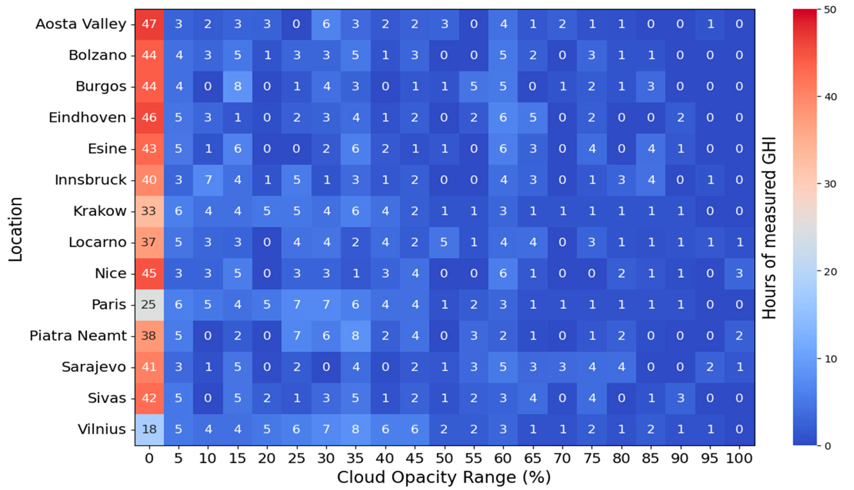
This section presents the findings from this study and discusses their implications for addressing challenges associated with data scarcity in solar energy prediction. This study highlights the potential effectiveness of the approach in optimizing the distribution of training data [40], as illustrated in Figure 3. By identifying the minimum number of hours of measured global horizontal irradiance (GHI) required for each sky condition to train the ML model, the effectiveness of this optimization strategy in enhancing model performance is analyzed. An emphasis is placed on the model’s preference for clear sky days during training and its broader impact on overall accuracy. The practical implications of the approach, including enhancements in equipment maintenance and data collection, are discussed. This study also evaluates the accuracy and reliability of the model, emphasizing the advantages of integrating synthetic data and augmentation techniques.

3.1. Preference for Clear Sky Days and Training Impact

As can be seen in Figure 3, various locations across Europe exhibit notable similarities in terms of hours of GHI for training with corresponding cloud opacity values. In particular, the model tends to select GHI data for training related to clear sky days (transparent opacity). This preference is derived from the simplicity and predictability of clear sky conditions, which offer stable and consistent relationships between weather quantities (such as solar angles, air temperature, and humidity) and GHI [41]. Clear sky days have less noise and fewer confounding factors, allowing models to achieve lower error rates and better generalization on unseen data [41]. This phenomenon is consistent with findings that ML models often perform better on regular and less noisy data [42,43]. The predictability of GHI is significantly higher under clear sky conditions [44], supporting the preference for clear sky data points [44].
Training on clear sky days improves the model’s overall performance, even when predicting GHI for all sky conditions (clear, intermittent, and overcast) [45,46]. By first learning the fundamental patterns from clear skies, the model builds a strong foundational understanding of the underlying physical relationships governing GHI [45,46]. This foundation allows the model to adapt more effectively to complex and variable patterns under intermittent and overcast conditions [45,46]. Training the model with GHI data associated with low cloud opacity values, i.e., clear sky conditions, helps identify and focus on the most relevant predictors without being negatively affected by noise, leading to a better initial model fit and robust generalization capabilities [42]. In essence, the model, by first mastering the easier clear sky examples, incrementally tackles more challenging cases through a form of active learning [40,47,48]. This staged learning process reduces the overall error for clear days, which may be more frequent, thus improving overall performance metrics.

3.2. Practical Implications and Data Collection

Our methodology can be seen as an important guide for selecting specific days in a year for instrument inspection, maintenance, and training data collection for ML models to ensure accurate predictions. This information helps to calibrate the instruments more accurately, thereby reducing the need for inspections throughout the year. It also makes equipment maintenance easier because it can be more precisely scheduled. By focusing on critical days for accurate predictions, proactive maintenance planning becomes more efficient, reducing unexpected downtime and ensuring consistent data accuracy. Such an approach is potentially sustainable and cost-effective, making it possible to save considerably and thereby minimizing any waste.
In addition, our approach also has benefits in terms of data collection. It minimizes the amount of work required for collecting data by concentrating on those days with specific sky conditions that are essential for obtaining accurate predictions [49]. This streamlined approach hints at potential optimizations in the allocation of time and resources, which could result in a more cost-effective process. This is especially relevant in remote or hard-to access locations where data collection can be resource-intensive [50]. Additionally, improved data quality arises from the reduced influence of confounding variables like cloud cover or extreme weather conditions, which can introduce inaccuracies into the dataset [51]. These enhancements in data quality have the potential to elevate the accuracy and efficacy of GHI prediction. However, we should highlight that these advantages are currently theoretical and require further experimental validation and testing to confirm their real-world benefits.

3.3. Model Accuracy and Reliability

As regards the accuracy of the model, it achieved an R2 score ranging from 0.91 to 0.97 when evaluated against the 2021 testing dataset. This performance signifies a robust correlation between the predicted and actual GHI values, as evidenced in Table 3, which shows performance metrics under three different scenarios:
  • Random Distribution: with no guided distribution of the training data.
  • Best Distribution: with guided best distribution of the training data to improve model accuracy.
  • Synthetic Data: incorporating synthetic data to further enhance the model accuracy.
Furthermore, the low RMSE, MAE, and MBE values provide strong evidence of the quality of prediction accuracy. Notably, these metrics showcase a significant decrease in error rates when synthetic data with augmentation techniques are integrated, indicating a close alignment between our model’s predictions and actual GHI values.
Moreover, the uncertainties associated with the measurements, particularly those from the utilization of first- and second-class pyranometers, can be analyzed to better understand the accuracy level of the model. Considering the theoretically achievable daily uncertainty of hourly GHI at a 95% confidence level, the first-class pyranometers typically have an uncertainty of around ±8% and second-class pyranometers an uncertainty of around ±20% [52]. The ability of the proposed model to minimize error rates even in the presence of such uncertainties underscores its robustness and reliability in predicting GHI accurately across varying atmospheric conditions.
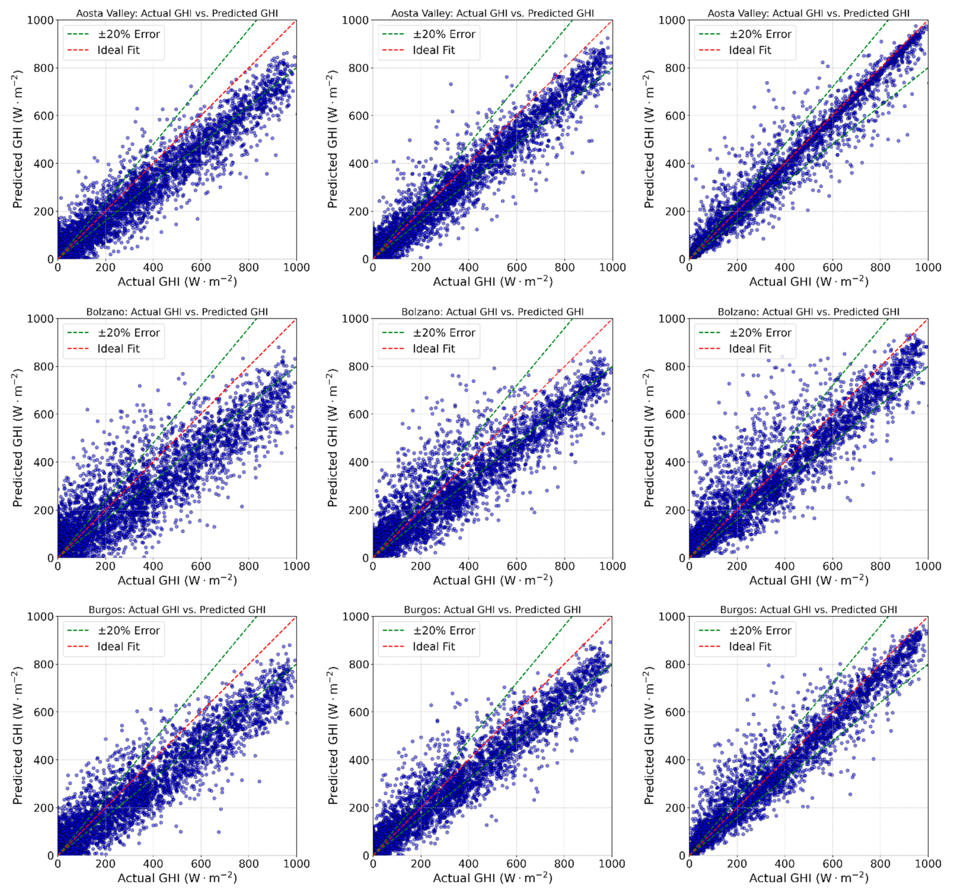
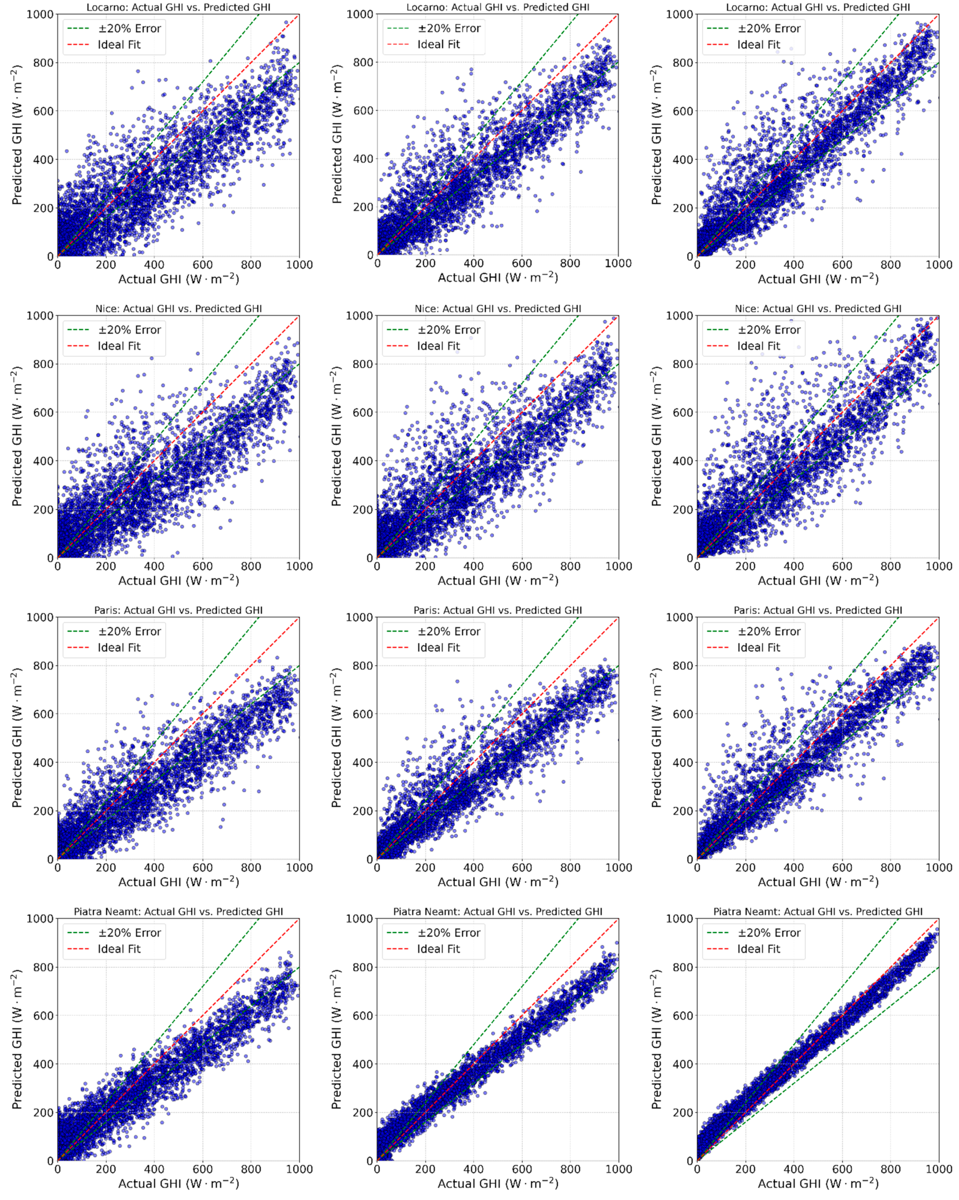
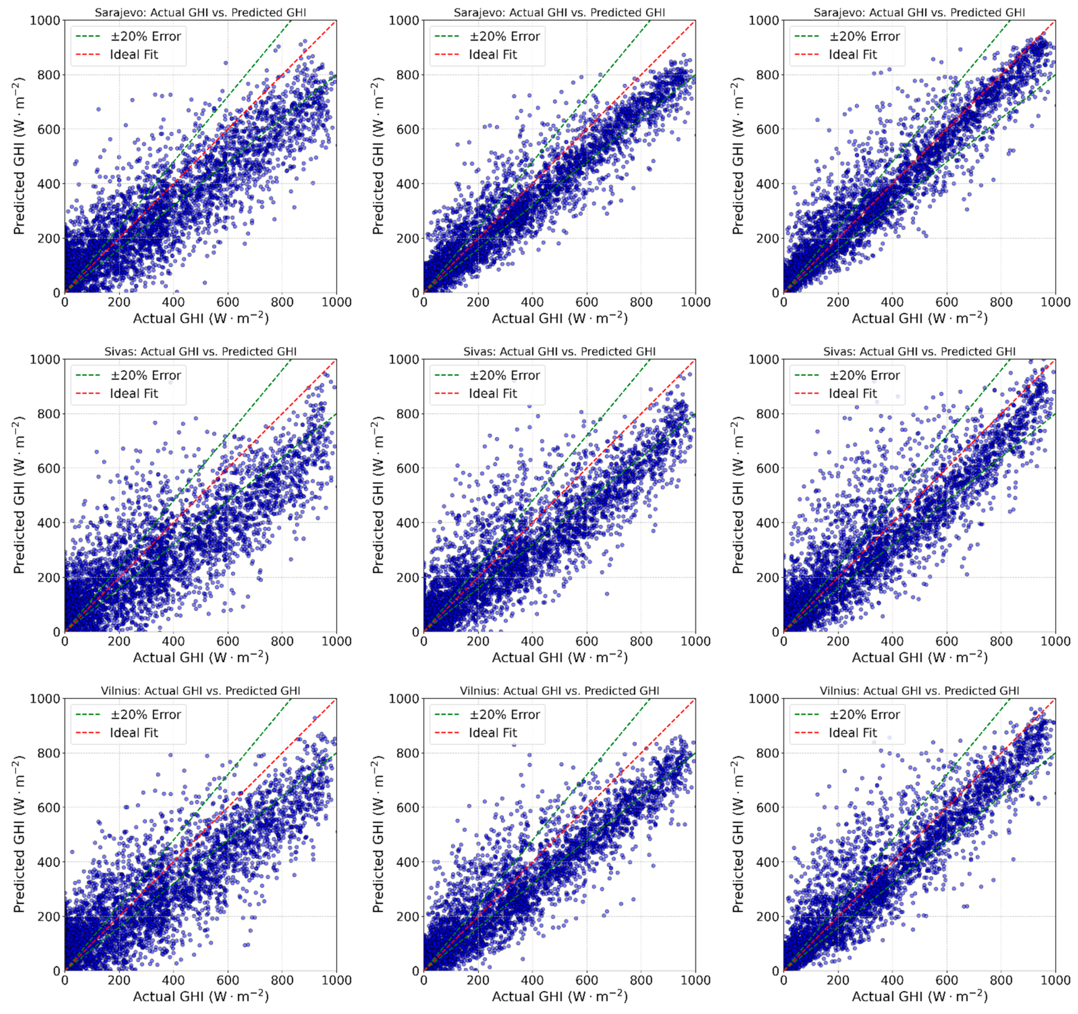
To illustrate the impact of our approach, Figure 4 includes scatter plots depicting the model’s performance under different training data scenarios: random distribution, best distribution, and synthetic data scenarios, focusing on predicted versus observed GHI values.
In the random distribution scenario, the scatterplot shows a wide dispersion of data points around the line of perfect agreement. This dispersion arises from the limited and less representative training data, particularly lacking critical hours of clear sky days. Consequently, the model struggles to predict accurately, resulting in significant errors.
Conversely, the best distribution scenario exhibits a tighter clustering of data points around the line of perfect agreement. Here, the training dataset includes a higher proportion of clear sky days, improving the model’s ability to generalize and predict GHI values more accurately, thus reducing errors.
The synthetic data scenario shows the least dispersion among the plots, with data points closely aligned with the line of perfect agreement. By leveraging synthetic data generation and augmentation techniques, this scenario effectively expands the training dataset. Augmenting the data enhances the model’s robustness and accuracy by exposing it to a broader range of conditions during training.
In summary, Figure 4 underscores the critical role of the training data quality and quantity in model performance. The random distribution scenario, constrained by limited and less representative data, leads to higher prediction errors. In contrast, the best distribution scenario, with strategically selected and representative data, significantly improves prediction accuracy. The synthetic data scenario further enhances accuracy through data augmentation, demonstrating the benefits of enlarging and diversifying the training dataset.
The inclusion of synthetic data generation and augmentation techniques has not only improved the model’s accuracy but also enhanced its reliability. By expanding our initial training dataset, the model now demonstrates improved predictive capabilities across various scenarios, including complex meteorological conditions such as those found in mountainous regions.

4. Conclusions

In conclusion, our study presents a cautiously optimistic approach for addressing the challenges posed by data scarcity in solar energy prediction. By integrating extreme gradient boosting (XGBoost) with random forest (RF) regression and employing active learning techniques, such as data sampling based on cloud opacity levels, and synthetic data generation and augmentation techniques, we have developed a methodology aimed at improving solar irradiance prediction.
Our results suggest the potential effectiveness of our approach in optimizing model performance across various locations in Europe and Asia Minor. By iteratively selecting GHI datapoints for model training and its corresponding predictors based on cloud opacity values, we have enhanced the model’s ability to make an accurate prediction of hourly GHI for all sky conditions. The integration of synthetic data generation and augmentation techniques to expand the training dataset has farther enhanced the model’s ability to make accurate predictions. Indeed, developed machine learning models achieved high accuracies, with an R2 score ranging from 0.91 to 0.97 and substantial reductions in RMSE, MAE, and MBE values, consistently across the selected locations. The findings also suggest that by optimizing the distribution of training data based on cloud opacity values, we may be able to identify specific days with favorable sky conditions for accurate GHI measurements.
The proposed approach has the potential to improve data collection efficiency, reduce costs, enhance data quality, and possibly aid in instrument calibration. For instance, our methodology may be considered for optimizing maintenance schedules, potentially reducing downtime, lowering maintenance costs, and extending the lifespan of equipment.
The proposed method has the potential to positively impact renewable energy generation by improving the accuracy of solar irradiance predictions. This could enable photovoltaic (PV) systems and solar water heaters to optimize operations, potentially leading to increased green energy production and more efficient resource use. These improvements support efforts to increase the share of renewable energy and reduce reliance on fossil fuels. More accurate predictions may help maximize efficiency, resulting in greater energy savings and potentially lower electricity bills.
Future research in this field could delve deeper into refining the synthetic data generation process, optimizing the integration of additional meteorological and environmental parameters, and extending the methodology to other regions. Additionally, testing the proposed methodology for predicting tilted irradiance (global tilted irradiance, GTI) is a crucial next step. Instead of focusing solely on cloud opacity, future studies should consider the distribution of training data based on sky cover and sunshine duration to further enhance prediction accuracy and reliability.

Author Contributions

Conceptualization, A.G. (Aleksandr Gevorgian), G.P. and A.G. (Andrea Gasparella); Methodology, A.G. (Aleksandr Gevorgian); Software, A.G. (Aleksandr Gevorgian); Resources, G.P.; Writing—original draft, A.G. (Aleksandr Gevorgian); Writing—review & editing, G.P. and A.G. (Andrea Gasparella); Supervision, G.P. and A.G. (Andrea Gasparella); Funding acquisition, A.G. (Andrea Gasparella). All authors have read and agreed to the published version of the manuscript.

Funding

This research was funded by the internal project of the Free University of Bozen-Bolzano “SOMNE—Bolzano Solar Irradiance Monitoring Network” (CUP: I56C18000930005; CRC Call 2018).

Data Availability Statement

The data presented in this study are available on request from the corresponding author.

Conflicts of Interest

The authors declare that this research was conducted in the absence of any commercial or financial relationships that could be construed as potential conflicts of interest.

References

  1. International Energy Agency. Solar PV. In Renewables 2020 Analysis and Forecast to 2025; IEA Publications: Paris, France, 2020; pp. 36–38. [Google Scholar]
  2. Allal, Z.; Noura, H.N.; Chahine, K. Machine Learning Algorithms for Solar Irradiance Prediction: A Recent Comparative Study. e-Prime-Adv. Electr. Eng. Electron. Energy 2024, 7, 100453. [Google Scholar] [CrossRef]
  3. Kamil, R.; Garniwa, P.M.P.; Lee, H. Performance Assessment of Global Horizontal Irradiance Models in All-Sky Conditions. Energies 2021, 14, 7939. [Google Scholar] [CrossRef]
  4. de Sá Campos, M.H.; Tiba, C. Global Horizontal Irradiance Modeling for All Sky Conditions Using an Image-Pixel Approach. Energies 2020, 13, 6719. [Google Scholar] [CrossRef]
  5. Kalogirou, S.A. Solar Energy Engineering: Processes and Systems, 2nd ed.; Academic Press: San Diego, CA, USA, 2013; pp. 45–67. [Google Scholar]
  6. Maisanam, A.; Podder, B.; Sharma, K.K.; Biswas, A. Solar Resource Assessment Using GHI Measurements at a Site in Northeast India. In Advances in Mechanical Engineering, Lecture Notes in Mechanical Engineering; Springer: Singapore, 2020; pp. 1253–1265. [Google Scholar]
  7. El Alani, O.; Ghennioui, H.; Abraim, M.; Ghennioui, A.; Blanc, P.; Saint-Drenan, Y.-M.; Naimi, Z. Solar Energy Resource Assessment Using GHI and DNI Satellite Data for Moroccan Climate. In Proceedings of the International Conference on Advanced Technologies for Humanity, Lecture Notes on Data Engineering and Communications Technologies, Rabat, Morocco, 26–27 November 2021; Springer: Cham, Switzerland, 2022; pp. 275–285. [Google Scholar]
  8. Ashenfelter, O.; Storchmann, K. Using Hedonic Models of Solar Radiation and Weather to Assess the Economic Effect of Climate Change: The Case of Mosel Valley Vineyards. Rev. Econ. Stat. 2010, 92, 333–349. [Google Scholar] [CrossRef]
  9. Srećković, V.A. New Challenges in Exploring Solar Radiation: Influence, Consequences, Diagnostics, Prediction. Appl. Sci. 2023, 13, 4126. [Google Scholar] [CrossRef]
  10. Zhu, T.; Guo, Y.; Li, Z.; Wang, C. Solar Radiation Prediction Based on Convolution Neural Network and Long Short-Term Memory. Energies 2021, 14, 8498. [Google Scholar] [CrossRef]
  11. Radhoush, S.; Whitaker, B.M.; Nehrir, H. An Overview of Supervised Machine Learning Approaches for Applications in Active Distribution Networks. Energies 2023, 16, 5972. [Google Scholar] [CrossRef]
  12. Hissou, H.; Benkirane, S.; Guezzaz, A.; Azrour, M.; Beni-Hssane, A. A Novel Machine Learning Approach for Solar Radiation Estimation. Sustainability 2023, 15, 10609. [Google Scholar] [CrossRef]
  13. Peng, T.; Li, Y.; Song, Z.; Fu, Y.; Nazir, M.S.; Zhang, C. Hybrid Intelligent Deep Learning Model for Solar Radiation Forecasting Using Optimal Variational Mode Decomposition and Evolutionary Deep Belief Network—Online Sequential Extreme Learning Machine. J. Build. Eng. 2023, 76, 107227. [Google Scholar] [CrossRef]
  14. Yadav, A.K.; Chandel, S.S. Solar Radiation Prediction Using Artificial Neural Network Techniques: A Review. Renew. Sustain. Energy Rev. 2014, 33, 772–781. [Google Scholar] [CrossRef]
  15. Kumar, R.; Aggarwal, R.K.; Sharma, J.D. Comparison of Regression and Artificial Neural Network Models for Estimation of Global Solar Radiations. Renew. Sustain. Energy Rev. 2015, 52, 1294–1299. [Google Scholar] [CrossRef]
  16. Pedro, H.T.C.; Coimbra, C.F.M. Assessment of Forecasting Techniques for Solar Power Production with No Exogenous Inputs. Sol. Energy 2012, 86, 2017–2028. [Google Scholar] [CrossRef]
  17. Dong, Z.; Yang, D.; Reindl, T.; Walsh, W.M. A Novel Hybrid Approach Based on Self-Organizing Maps, Support Vector Regression and Particle Swarm Optimization to Forecast Solar Irradiance. Energy 2015, 82, 570–577. [Google Scholar] [CrossRef]
  18. Voyant, C.; Notton, G.; Kalogirou, S.; Nivet, M.-L.; Paoli, C.; Motte, F.; Fouilloy, A. Machine Learning Methods for Solar Radiation Forecasting: A Review. Renew. Energy 2017, 105, 569–582. [Google Scholar] [CrossRef]
  19. Elizabeth Michael, N.; Mishra, M.; Hasan, S.; Al-Durra, A. Short-Term Solar Power Predicting Model Based on Multi-Step CNN Stacked LSTM Technique. Energies 2022, 15, 2150. [Google Scholar] [CrossRef]
  20. Alharkan, H.; Habib, S.; Islam, M. Solar Power Prediction Using Dual Stream CNN-LSTM Architecture. Sensors 2023, 23, 945. [Google Scholar] [CrossRef] [PubMed]
  21. Whang, S.E.; Roh, Y.; Song, H.; Lee, J.G. Data Collection and Quality Challenges in Deep Learning: A Data-Centric AI Perspective. VLDB J. 2023, 32, 791–813. [Google Scholar] [CrossRef]
  22. Sai Srinivas, T.A.; Thanmai, B.T.; Donald, A.D.; Thippanna, G.; Srihith, I.V.D.; Sai, I.V. Training Data Alchemy: Balancing Quality and Quantity in Machine Learning Training. J. Netw. Secur. Data Min. 2023, 6, 7–10. [Google Scholar] [CrossRef]
  23. Budach, L.; Feuerpfeil, M.; Ihde, N.; Nathansen, A.; Noack, N.; Patzlaff, H.; Naumann, F.; Harmouch, H. The Effects of Data Quality on Machine Learning Performance. arXiv 2022, arXiv:2207.14529. [Google Scholar] [CrossRef]
  24. Quach, S.; Thaichon, P.; Martin, K.D.; Weaven, S.; Palmatier, R.W. Digital Technologies: Tensions in Privacy and Data. J. Acad. Mark. Sci. 2022, 50, 1299–1323. [Google Scholar] [CrossRef]
  25. Ju, W.; Yi, S.; Wang, Y.; Xiao, Z.; Mao, Z.; Li, H.; Gu, Y.; Qin, Y.; Yin, N.; Wang, S.; et al. A Survey of Graph Neural Networks in Real World: Imbalance, Noise, Privacy and OOD Challenges. arXiv 2024, arXiv:2403.04468. [Google Scholar] [CrossRef]
  26. Wang, J.; Liu, Y.; Li, P.; Lin, Z.; Sindakis, S.; Aggarwal, S. Overview of Data Quality: Examining the Dimensions, Antecedents, and Impacts of Data Quality. J. Knowl. Econ. 2024, 15, 1159–1178. [Google Scholar] [CrossRef]
  27. Subramanian, E.; Karthik, M.M.; Krishna, G.P.; Prasath, D.V.; Kumar, V.S. Solar Power Prediction Using Machine Learning. arXiv 2023, arXiv:2303.07875. [Google Scholar] [CrossRef]
  28. Breiman, L. Random Forests. Mach. Learn. 2001, 45, 5–32. [Google Scholar] [CrossRef]
  29. Chen, T.; Guestrin, C. XGBoost: A Scalable Tree Boosting System. In Proceedings of the 22nd ACM SIGKDD International Conference on Knowledge Discovery and Data Mining, San Francisco, CA, USA, 13–17 August 2016; ACM: New York, NY, USA, 2016; pp. 785–794. [Google Scholar]
  30. Bright, J.M. Solcast: Validation of a Satellite-Derived Solar Irradiance Dataset. Sol. Energy 2019, 189, 435–449. [Google Scholar] [CrossRef]
  31. Solcast. Irradiance and Weather Data: How Solcast Generates Irradiance and Weather Data. Available online: https://solcast.com/irradiance-data-methodology (accessed on 13 May 2024).
  32. Maharana, K.; Mondal, S.; Nemade, B. A Review: Data Pre-processing and Data Augmentation Techniques. Glob. Transit. Proc. 2022, 3, 91–99. [Google Scholar] [CrossRef]
  33. Topographic-Map. Topographic Maps and Satellite Images. Topographic-Map.com 2024. Available online: https://en-us.topographic-map.com/ (accessed on 19 May 2024).
  34. Visual Crossing. Weather Data Services. Visual Crossing 2024. Available online: https://www.visualcrossing.com/weather/weather-data-services (accessed on 13 May 2024).
  35. Solcast. Global Solar Irradiance Data and PV System Power Output Data. Solcast 2024. Available online: https://solcast.com/data-for-researchers (accessed on 13 May 2024).
  36. El-Amarty, N.; Marzouq, M.; El Fadili, H.; Dosse Bennani, S.; Ruano, A. A Comprehensive Review of Solar Irradiation Estimation and Forecasting Using Artificial Neural Networks: Data, Models and Trends. Environ. Sci. Pollut. Res. 2023, 30, 5407–5439. [Google Scholar] [CrossRef] [PubMed]
  37. Pedro, H.T.C.; Larson, D.P.; Coimbra, C.F.M. A Comprehensive Dataset for the Accelerated Development and Benchmarking of Solar Forecasting Methods. J. Renew. Sustain. Energy 2019, 11, 036102. [Google Scholar] [CrossRef]
  38. Guzman, R.; Chepfer, H.; Noel, V.; Vaillant de Guélis, T.; Kay, J.E.; Raberanto, P.; Cesana, G.; Vaughan, M.A.; Winker, D.M. Direct Atmosphere Opacity Observations from CALIPSO Provide New Constraints on Cloud-Radiation Interactions. J. Geophys. Res. Atmos. 2017, 122, 1066–1085. [Google Scholar] [CrossRef]
  39. S’COOL. Cloud Visual Opacity. NASA Globe 2024. Available online: https://www.globe.gov/web/s-cool/home/observation-and-reporting/cloud-visual-opacity (accessed on 19 May 2024).
  40. Settles, B.; Active Learning Literature Survey. Computer Sciences Technical Report 1648. 2010. Available online: https://burrsettles.com/pub/settles.activelearning.pdf (accessed on 20 May 2024).
  41. Mendyl, A.; Mabasa, B.; Bouzghiba, H.; Weidinger, T. Calibration and Validation of Global Horizontal Irradiance Clear Sky Models against McClear Clear Sky Model in Morocco. Appl. Sci. 2023, 13, 320. [Google Scholar] [CrossRef]
  42. Poulinakis, K.; Drikakis, D.; Kokkinakis, I.W.; Spottswood, S.M. Machine-Learning Methods on Noisy and Sparse Data. Mathematics 2023, 11, 236. [Google Scholar] [CrossRef]
  43. Reis, I.; Baron, D.; Shahaf, S. Probabilistic Random Forest: A Machine Learning Algorithm for Noisy Data Sets. Astron. J. 2019, 157, 16. [Google Scholar] [CrossRef]
  44. Jiménez, P.A.; Alessandrini, S.; Haupt, S.E.; Deng, A.; Kosovic, B.; Lee, J.A.; Delle Monache, L. The Role of Unresolved Clouds on Short-Range Global Horizontal Irradiance Predictability. Mon. Weather Rev. 2016, 144, 3099–3107. [Google Scholar] [CrossRef]
  45. Al-lahham, A.; Theeb, O.; Elalem, K.; Alshawi, T.A.; Alshebeili, S.A. Sky Imager-Based Forecast of Solar Irradiance Using Machine Learning. arXiv 2020, arXiv:2310.17356. Available online: https://arxiv.org/pdf/2310.17356 (accessed on 25 May 2024).
  46. Nie, Y.; Paletta, Q.; Scott, A.; Pomares, L.M.; Arbod, G.; Sgouridis, S.; Lasenby, J.; Brandt, A. Sky Image-Based Solar Forecasting Using Deep Learning with Multi-Location Data: Training Models Locally, Globally or via Transfer Learning? arXiv 2022, arXiv:2211.02108. Available online: https://arxiv.org/pdf/2211.02108 (accessed on 25 May 2024).
  47. Vasanthakumari, P.; Zhu, Y.; Brettin, T.; Partin, A.; Shukla, M.; Xia, F.; Narykov, O.; Weil, M.R.; Stevens, R.L. A Comprehensive Investigation of Active Learning Strategies for Conducting Anti-Cancer Drug Screening. Cancers 2024, 16, 530. [Google Scholar] [CrossRef] [PubMed]
  48. Hino, H. Active Learning: Problem Settings and Recent Developments. arXiv 2020, arXiv:2012.04225. [Google Scholar] [CrossRef]
  49. Zellweger, F.; Sulmoni, E.; Malle, J.T.; Baltensweiler, A.; Jonas, T.; Zimmermann, N.E.; Ginzler, C.; Karger, D.N.; De Frenne, P.; Frey, D.; et al. Microclimate Mapping Using Novel Radiative Transfer Modeling. Biogeosciences 2024, 21, 605–623. [Google Scholar] [CrossRef]
  50. Ohler, L.M.; Lechleitner, M.; Junker, R.R. Microclimatic Effects on Alpine Plant Communities and Flower-Visitor Interactions. Sci. Rep. 2020, 10, 1366. [Google Scholar] [CrossRef]
  51. Krishnan, N.; Kumar, K.R.; Inda, C.S. How Solar Radiation Forecasting Impacts the Utilization of Solar Energy: A Critical Review. J. Clean. Prod. 2023, 388, 135860. [Google Scholar] [CrossRef]
  52. Solargis. Combining Model Uncertainty and Interannual Variability. Available online: https://solargis.com/docs/accuracy-and-comparisons/combining-model-uncertainty-and-interannual-variability (accessed on 19 May 2024).
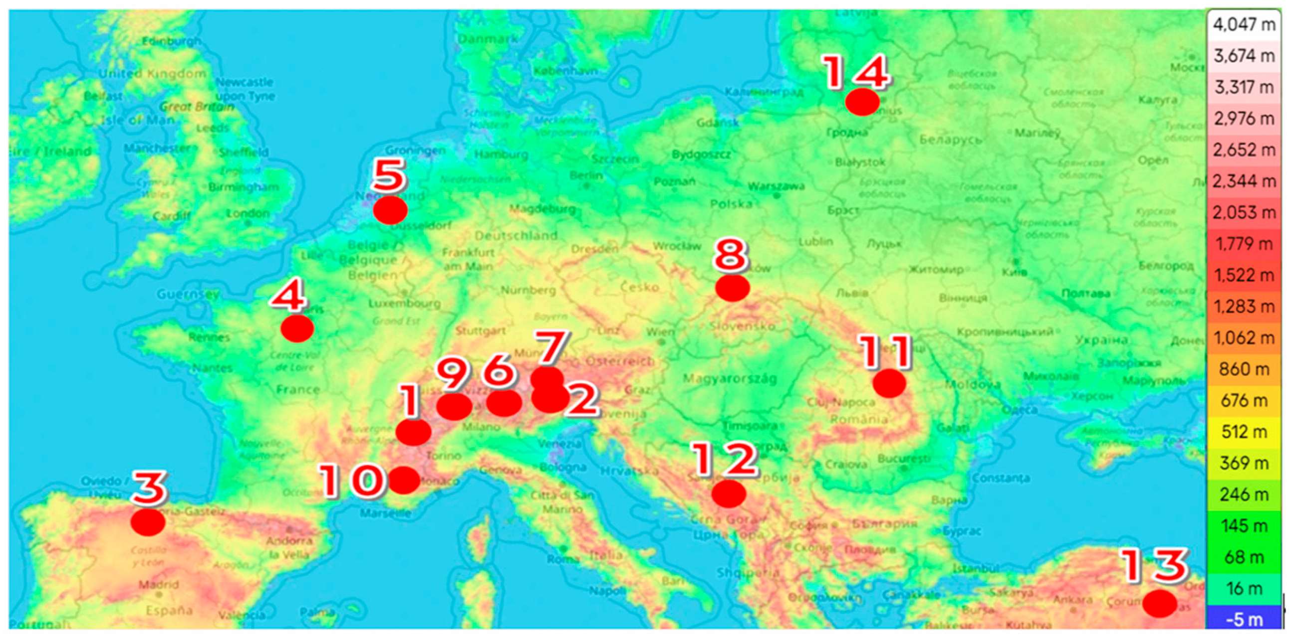
Figure 1. Spatial distribution of training and testing sites for global horizontal irradiance (GHI) prediction model. The map indicates terrain complexity with varying altitudes for each location. Map generated from the available source [33]. See Table 1 for the names of locations (1–14) and further data.
Energies 17 03365 g001
Figure 2. Example of random forest decision tree structure.
Energies 17 03365 g002
Figure 3. Cloud opacity range and corresponding hours of measured GHI selected for model training.
Energies 17 03365 g003
Figure 4. Comparative scatterplots of model performance (from left to right): random distribution, best distribution, and synthetic data scenarios.
Energies 17 03365 g004aEnergies 17 03365 g004bEnergies 17 03365 g004cEnergies 17 03365 g004d
Table 1. Spatial sampling sites for model training and testing.
Station Code NameSiteCountyLatitude (°)Longitude (°)Altitude (m)
1EW5468 Saint-Christophe Aosta ValleyItaly45.757.343951
2UniBZBolzanoItaly46.5011.35262
3LEBGBurgosSpain42.37−3.63859
4CW1292 Coignieres FRParisFrance48.8122.27628
5EHEHEindhovenNetherlands51.455.4217
6IW2LAO-13 Esine ITEsineItaly45.9210.25286
7LOWIInnsbruckAustria47.2711.35574
8EPKKKrakowPoland50.0819.8219
9LSZLLocarnoSwitzerland46.168.88200
10LFMNNiceFrance43.657.24
11YO8RBY-13 Piatra Neamt Piatra NeamtRomania46.9626.387345
12LQSASarajevoBosnia–Herzegovina43.8218.32518
13LTARSivasTurkey39.7936.91285
14EYVIVilniusLithuania54.6325.28112
Table 2. Environmental, solar geometry, and temporal variables for model training and testing.
VariableDescriptionUnits
GHIThe total amount of shortwave radiation received from above by a surface horizontal to the groundW·m−2
Air temperatureThe temperature of the air°C
AzimuthThe angle between the projected vector of the sun on the ground and a reference vector on that grounddegrees
Cloud opacityThe thickness or density of clouds affecting sunlight%
Dew point temperatureThe temperature at which air must be cooled to become saturated with water vapor°C
Precipitable waterThe total atmospheric water vapor contained in a vertical column of unit cross-sectional areakg·m−2
Relative humidityThe amount of water vapor present in air expressed as a percentage of the amount needed for saturation at the same temperature%
Surface pressureThe pressure exerted by the atmosphere at the earth’s surfacehPa
Wind direction 10 mThe direction from which the wind is blowing at 10 m above the surfacedegrees
Wind speed 10 mThe speed of the wind measured at 10 m above the surfacem·s−1
ZenithThe angle away from the vertical direction to the sun at its highest pointdegrees
MonthThe month of the year-
DayThe day of the month-
HoursThe hour of the day in 24 h format-
Table 3. Performance metrics for GHI prediction with and without synthetic data generation and augmentation techniques.
CityScenarioR2RMSE
[W m−2]
MAE
[W m−2]
MBE
[W m−2]
Aosta ValleyRandom Distribution0.8499.7571.3639.03
Best Distribution0.9368.1648.2520.10
Synthetic Data0.9742.6420.333.13
BolzanoRandom Distribution0.79114.9378.6138.58
Best Distribution0.8887.9057.7720.57
Synthetic Data0.9174.6141.823.06
BurgosRandom Distribution0.83103.4772.9739.14
Best Distribution0.9173.7450.6920.74
Synthetic Data0.9652.9329.073.32
EindhovenRandom Distribution0.81107.8877.8338.80
Best Distribution0.9176.2653.8819.71
Synthetic Data0.9553.5228.903.16
EsineRandom Distribution0.80110.5873.9338.80
Best Distribution0.8886.2558.8719.93
Synthetic Data0.9366.4038.623.12
InnsbruckRandom Distribution0.81108.1173.9638.71
Best Distribution0.8982.9655.7620.78
Synthetic Data0.9367.8439.533.00
KrakowRandom Distribution0.8694.8865.2939.11
Best Distribution0.9268.8747.5719.52
Synthetic Data0.9745.9319.033.06
LocarnoRandom Distribution0.80111.7577.7738.73
Best Distribution0.8888.4261.6820.25
Synthetic Data0.9269.9738.423.06
NiceRandom Distribution0.78118.1880.6529.05
Best Distribution0.8498.5667.609.63
Synthetic Data0.8887.3153.51−9.07
ParisRandom Distribution0.78118.0983.2443.98
Best Distribution0.9080.5251.2824.72
Synthetic Data0.9462.6231.737.56
Piatra NeamtRandom Distribution0.8694.7568.1827.66
Best Distribution0.9458.9544.316.49
Synthetic Data0.9740.0332.57−11.89
SarajevoRandom Distribution0.84101.4969.5836.15
Best Distribution0.9271.0145.8916.49
Synthetic Data0.9459.4633.62−1.01
SivasRandom Distribution0.75124.1887.0941.58
Best Distribution0.8597.6464.3723.78
Synthetic Data0.8984.3046.386.93
VilniusRandom Distribution0.78117.4783.7839.59
Best Distribution0.8886.9858.9320.38
Synthetic Data0.9271.5339.863.12
Disclaimer/Publisher’s Note: The statements, opinions and data contained in all publications are solely those of the individual author(s) and contributor(s) and not of MDPI and/or the editor(s). MDPI and/or the editor(s) disclaim responsibility for any injury to people or property resulting from any ideas, methods, instructions or products referred to in the content.