Single-Sensor Global MPPT for PV System Interconnected with DC Link Using Recent Red-Tailed Hawk Algorithm

Abstract

The primary disadvantage of solar photovoltaic systems, particularly in partial shadowing conditions (PSC), is their low efficiency. A power–voltage curve with a homogenous distribution of solar irradiation often has a single maximum power point (MPP). Without a doubt, it can be extracted using any conventional tracker—for instance, perturb and observe. On the other hand, under PSC, the situation is entirely different since, depending on the number of distinct solar irradiation levels, the power–voltage curve has numerous MPPs (i.e., multiple local points and one global point). Conventional MPPTs can only extract the first point since they are unable to distinguish between local and global MPP. Thus, to track the global MPP, an optimized MPPT based on optimization algorithms is needed. The majority of global MPPT techniques seen in the literature call for sensors for voltage and current in addition to, occasionally, temperature and/or solar irradiance, which raises the cost of the system. Therefore, a single-sensor global MPPT based on the recent red-tailed hawk (RTH) algorithm for a PV system interconnected with a DC link operating under PSC is presented. Reducing the number of sensors leads to a decrease in the cost of a controller. To prove the superiority of the RTH, the results are compared with several metaheuristic algorithms. Three shading scenarios are considered, with the idea of changing the shading scenario to change the location of the global MPP to measure the consistency of the algorithms. The results verified the effectiveness of the suggested global MPPT based on the RTH in precisely capturing the global MPP compared with other methods. As an example, for the first shading situation, the mean PV power values varied between 6835.63 W and 5925.58 W. The RTH reaches the highest PV power of 6835.63 W flowing through particle swarm optimization (6808.64 W), whereas greylag goose optimizer achieved the smallest PV power production of 5925.58 W.

1. Introduction

Renewable energy sources are becoming more appealing due to environmental issues like climate change, global warming, and the depletion of fossil fuels [1]. The use of fossil fuels, civilization, and human density are all contributing to the planet’s rapid temperature rise [2]. To counteract global warming, researchers are looking at renewable energy sources. A viable, noise- and pollution-free alternative is solar energy. To maximize energy conversion efficiency and cut costs, effective strategies are required [3].

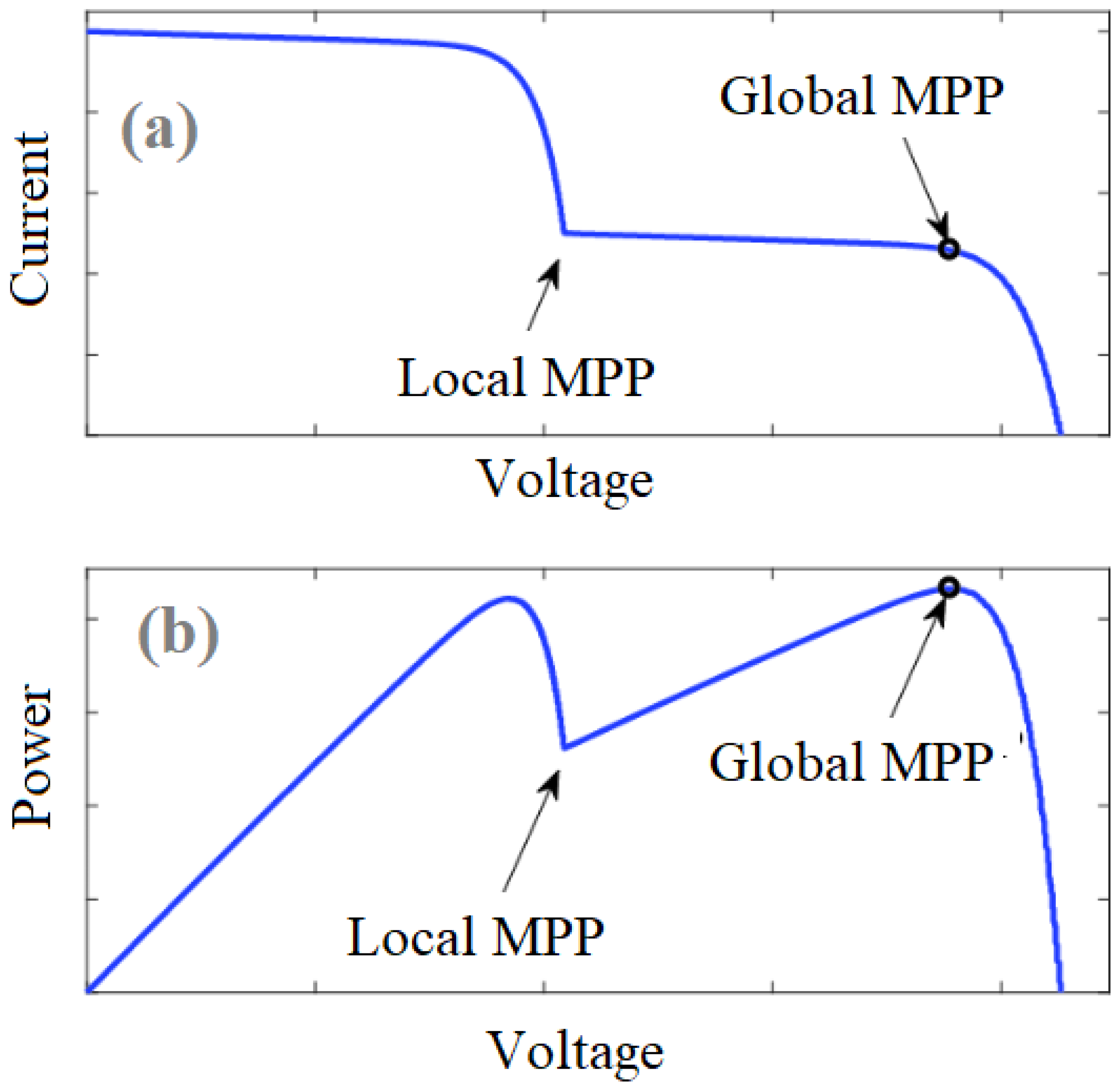
The abundance and environmental friendliness of renewable energy technologies, particularly photovoltaic (PV) energy, have drawn increased attention recently. Temperature and irradiance are two climatic factors that affect photovoltaic system generation [4]. A control circuit must be inserted to operate the PV panels during the voltage that results in the peak point since the relationship between the PV output voltage and generated power is nonlinear and has only one peak power. This can be achieved by using a DC-to-DC converter controlled by a maximum point tracker (MPPT). The most popular and straightforward MPPT technologies are hill climbing, incremental conductance, and perturb and observe. Nonetheless, there are several drawbacks to employing these conventional technologies, particularly when the PV system is operating in partial shadow, as the power–voltage curve in this scenario has a single global peak and numerous local peaks [5]. In these conditions, conventional technologies might detect a local peak and interpret it as the global peak. This would result in an increase in the output power loss and a decrease in the use of the PV generator. Thus, to avoid catching the local peak from the system, methods with a strong search ability are crucial. These methods, referred to as global MPPTs.

Optimization algorithms have been used in different applications in addition to the global MPPT. A hybrid optimization method comprising an ant lion optimizer and a neural network was developed by Alblawi et al. [6] for forecasting the PV cell temperature and output power. To maximize the microgrid resilience, a two-stage AI-enhanced system with an integrated backup system based on a hybrid optimization algorithm has been proposed by Elkholy et al. [7]. To track the global MPP obtained from the PV system at PSC, a bio-inspired whale optimization approach was introduced [8]. The approach’s performance was enhanced by reinitializing it. To improve the PV-system-generated power under quickly changing shading conditions, a control scheme representing an MPPT integrated between a fractional P&O tracker and fractional proportional–integral controller has been established in [9].

Additionally, the hunter–prey optimizer was used to determine the settings of the controller that was supplied. The authors of [10] presented a modified version of the tunicate swarm method to improve the PV system performance by tracking the global MPP. Two random integers were added to the method throughout its update process to improve the search functionality. By comparing the expected peak with the global peak, a tracker based on the fly search agent approach has been given to detect the global peak of the PV system during shading circumstances [11]. To evaluate the created tracker, benchmark shading patterns have also been examined. An enhanced algorithm that is accessible during abrupt weather changes has been introduced to address the long-term tracking issue related to the usage of the conventional power feedback approach in determining the maximum power from PV modules/arrays [12]. Eltamaly [13] proposed a new global MPPT method using a musical chairs algorithm for MPPT PV applications. The results demonstrated that the convergence time was decreased to 20–50% of those attained by another benchmark algorithms.

Typically, parallel connections between the PV module and switched bypass diodes are possible. Normal circumstances have no effect on these diodes [14]. When shadowing occurs, the bypass diodes become backward biased and transmit the current rather than the PV module. Because of this, a PV system’s power–voltage curve under partially shadowed conditions has a single global point and multiple local MPPs. Therefore, it is imperative to track such a global maximum point. Consequently, under shading, the efficacy of conventional MPPT techniques is diminished [15]. The distinction between the global and local peaks cannot be made using conventional MPPT techniques, such as hill climbing and incremental conductance. Therefore, the effectiveness of tracking MPP under shading is lowered as a result. To extract the global MPP in this scenario, several global MPPT approaches based on modern optimization have been devised. Among these algorithms are the following: the grey wolf optimizer [16], hybrid cuckoo search and artificial bee colony [17], mine blast optimization [18], and teaching–learning-based optimization [19].

Therefore, in this paper, a single-sensor global MPPT based on the recent red-tailed hawk (RTH) algorithm for a PV system interconnected with a DC link operating under PSC is presented. To prove the superiority of the RTH, the results are compared with another ten algorithms including bald eagle search (BES), modified bald eagle search (mBES), the blue monkey algorithm (BMA), the black widow optimization algorithm (BWOA), greylag goose optimization (GGO), the grey wolf optimizer (GWO), Harris hawks optimization (HHO), the pelican optimization algorithm (POA), particle swarm optimization (PSO), and the whale optimization algorithm (WOA). Three shading scenarios are considered, with the idea of changing the shading scenario to change the location of the global MPP to measure the consistency of the algorithms.

2. PV Array under Shading

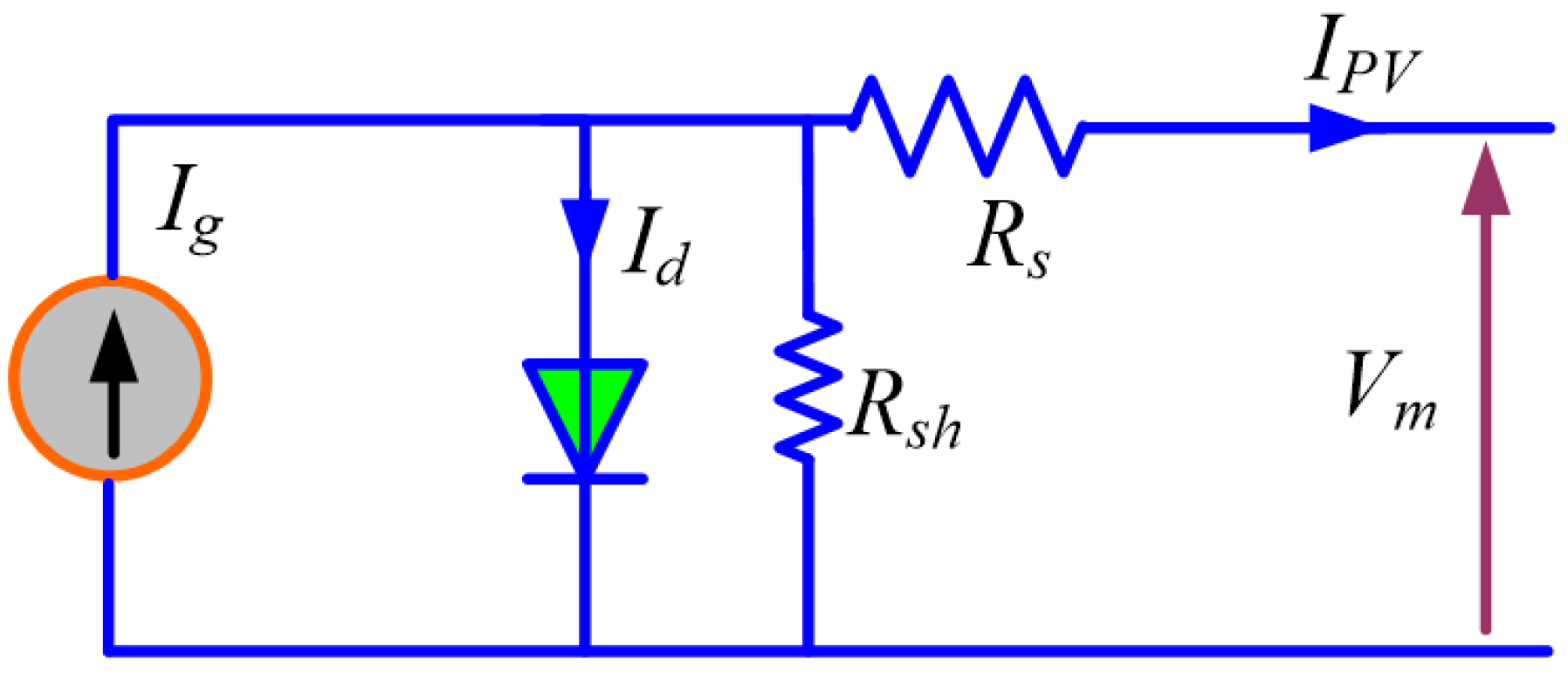
A single-diode model circuit is explained in Figure 1. The output current of the PV module is defined using the following relation [20]:

$$I=I_g-I_o\left[\mathit{exp}\left(\frac{q.\left(V_m+R_{s}I\right)}{aKT}\right)-1\right]-\left[\frac{V_m+R_{s}I}{R_{sh}}\right]$$

(1)

where $I_g$ presents the generated photo-current; $I_0$ presents the reverse saturation current; q presents the electron charge; $V_m$ and $I$ present the output current and the voltage of the solar cell, respectively; $a$ presents the ideality factor of the parallel diode and depends on the semiconductor device; K is the Boltzmann constant; and $R_s$ and $R_{sh}$ are the series and shunt resistances, respectively.

Figure 1. Solar cell single-diode model.

The photon current relies on the intensity of the solar radiation and temperature. The following formula is used to calculate it [20]:

$$I_g=I_{sc0}\left(\frac{G}{G_0}\right)\left(1+{\beta }_i\left(T-T_0\right)\right)\left(\frac{R_s+R_{sh}}{R_{sh}}\right)$$

(2)

where $I_{sc0}$ is the short-circuit current; $T_0$ and $G_0$ are the temperature and irradiance at STC, respectively; $T$ is the ambient temperature; G is the ambient irradiance; and ${\beta }_i$ presents the current temperature coefficient.

Partial shadowing is a frequently anticipated event for large-scale photovoltaic systems. The shade from surrounding trees, structures, birds, or bird droppings is a major problem that affects the operation of PV systems [20]. One of the main factors reducing the PV system’s output power is shadowing, whether it is full or partial. PSC happens when shadows cast by other PV modules, buildings, clouds, or even other PV modules themselves cover the modules. Bypass diodes can be used to mitigate the shade temporarily and shield the PV system from malfunctioning. A diode can be used to provide an additional path for the PV current to follow when a cell is broken or shaded [21]. It will barely affect the panel’s power and totally bypass any broken or darkened cells. To reduce the risk created by the hot-spot phenomenon, one or three bypass diodes are often attached per module [22]. The power against voltage curves of the PV array at the normal distribution of solar radiation and under shading are demonstrated in Figure 2. When the PV array operates at the normal distribution of solar radiation, its P–V curve has one MPP. This point can be easily obtained by any convention MPPT method. On the other side, at a partial shade operation, the P–V curve has several peaks. Global MPP can be tracked through installing MPPT based on modern optimization algorithms [23].

Figure 2. PV characteristics under shading: (a) current against voltage curve and (b) power against voltage curve.

3. Red-Tailed Hawk Algorithm

RTH is a recent optimization method that simulates the hunting behavior of red-tailed hawks. There are three essential phases of hunting as explained in Figure 3: the high-soaring, low-soaring, and swooping phases [24].

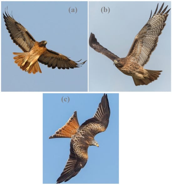
Figure 3. The three phases of the red-tailed hawk during hunting process: (a) high-soaring, (b) low-soaring, and (c) stopping and swooping.

1.

The first phase (high-soaring): In this phase, the RTH is soaring high into the sky but far away from its target. This phase can be modeled as follows [24]:

$$x\left(k\right)=x_G+(x_{av}-x(k-1\left)\right)\cdot Levy(\mathit{Dim})\cdot TF(k)$$

(3)

where x(k) is the new location, x_G is the best location, and x_av is the average of all locations. TF(k) is the transition factor function. The levy flight distribution and TF may be estimated using (5) and (6):

$$\begin{gathered} Levy\left(\mathit{Dim}\right)=C_1\frac{r_1\cdot \sigma }{{\left|r_2\right|}^{{C_2}^{-1}}} \\ \sigma =\left(\frac{\Gamma (1+C_2)\cdot \mathit{sin}\left(\frac{\pi C_2}{2}\right)}{\Gamma (\frac{1+C_2}{2})\cdot C_2\cdot 2^{\left(\frac{1-C_2}{2}\right)}}\right) \end{gathered}$$

(4)

where $C_1$ and $C_2$ are constants; and $r_1$ and $r_2$ denote randoms.

$$TF(k)=1+\mathit{sin}\left(2.5+\left(\frac{k}{T_m}\right)\right)$$

(5)

where T_m denotes the maximum number of iterations.

2.

The second phase (low-soaring): The hawk comes much nearer to the prey. Considering a spiral movement for surrounding the prey, the new location can be defined as follows [24]:

$$\begin{array}{l}x(k+1)=x_G+\left(x\right(k)+y(k\left)\right)\cdot T_s\left(k\right)\\ T_s\left(k\right)=x\left(k\right)-x_{av}\end{array}$$

(6)

$$\begin{array}{ll}\left\{\begin{array}{c}x\left(k\right)=A\left(k\right)\cdot \mathit{sin}\left(\theta \left(k\right)\right)\\ y\left(k\right)=A\left(k\right)\cdot \mathit{cos}\left(\theta \left(k\right)\right)\end{array}\right.& \left\{\begin{array}{c}A(k)=A_0\cdot (g-{\displaystyle \frac{k}{T_m}}).r_3\\ \theta \left(k\right)=\varnothing \cdot \left(1-{\displaystyle \frac{k}{T_m}}\right).r_3\end{array}\right.\left\{\begin{array}{c}x(k)={\displaystyle \frac{x\left(k\right)}{\mathit{max}\left|x\left(k\right)\right|}}\\ y(k)={\displaystyle \frac{y\left(k\right)}{\mathit{max}\left|y\left(k\right)\right|}}\end{array}\right.\end{array}$$

(7)

where:

A₀ denotes the initial value of the radius that varies;

$\varnothing$ denotes the angle gain that varies;

$r_3$ denotes a random number;

g is a controlling factor.

3.

The third phase (stooping and swooping): The hawk rapidly drops its body to attack the prey. The modification of the location in this phase can be defined as follows [23]:

$$x\left(k\right)=\alpha \left(t\right)\cdot x_G+x\left(k\right)\cdot T_{s1}\left(k\right)+y\left(t\right)\cdot T_{s2}\left(k\right)$$

(8)

The steps’ sizes can be obtained according to the following:

$$\begin{array}{l}{T}_{s1}\left(k\right)=x\left(\mathrm{k}\right)-TF\left(k\right)\cdot x_{av}\\ T_{s2}\left(k\right)=G\left(k\right)\cdot x\left(k\right)-TF\left(k\right)\cdot x_G\end{array}$$

(9)

where α and G denote the accelerating and gravitational parameters, respectively.

$$\begin{array}{l}\alpha \left(k\right)={sin}^2\cdot \left(2.5-{\displaystyle \frac{k}{T_m}}\right)\\ G(k)=2\cdot \left(1-\frac{k}{T_m}\right)\end{array}$$

(10)

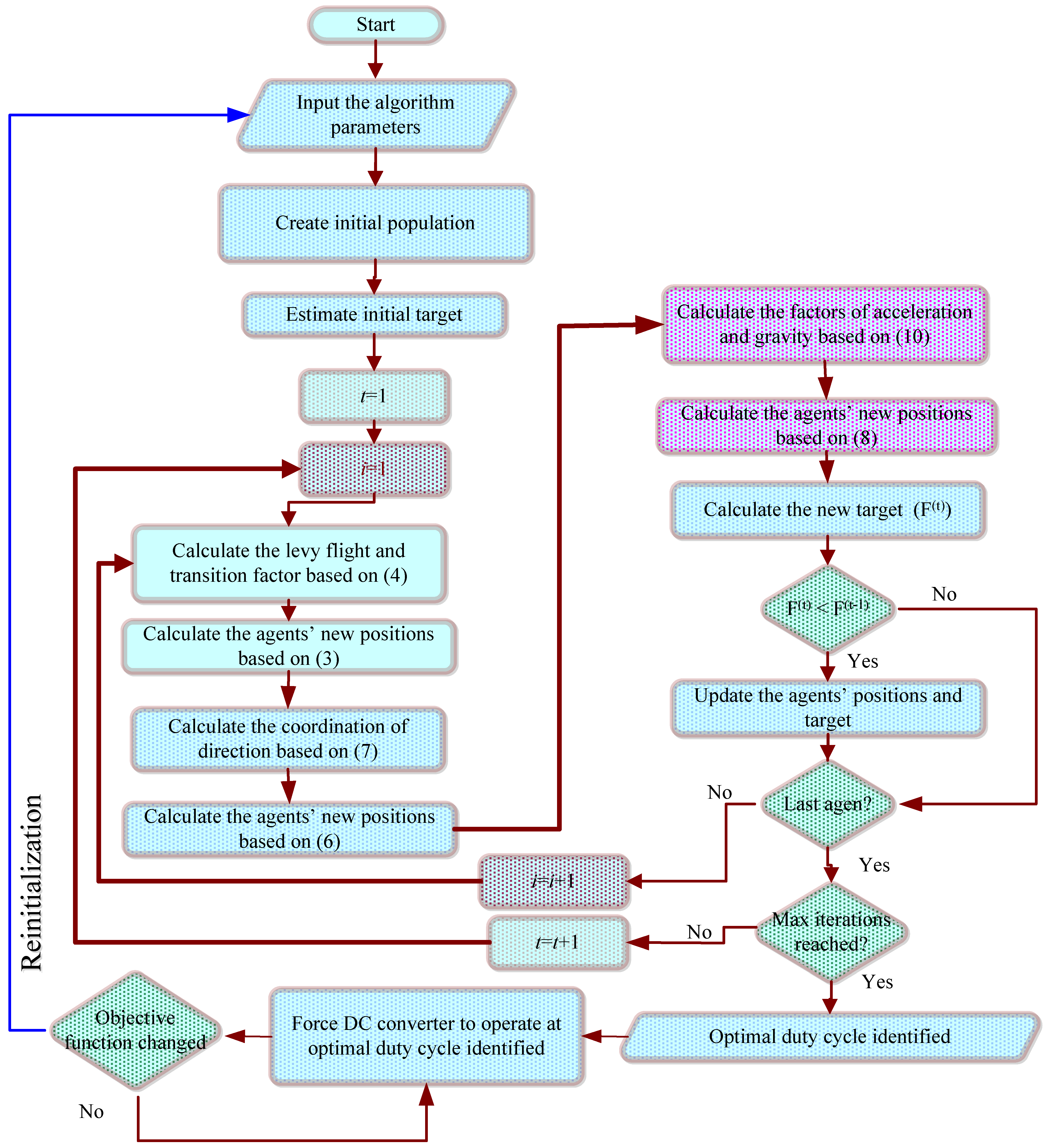
The steps of RTH-based MPPT is explained in Figure 4.

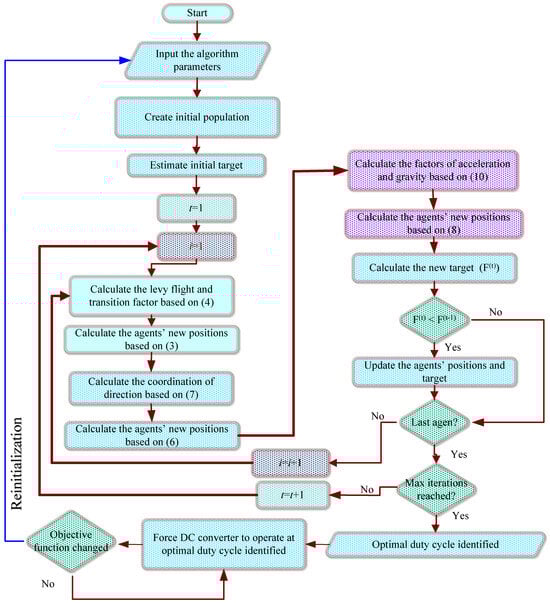
Figure 4. RTH-flowchart-based global MPPT.

4. Results and Discussion

The PV system interconnected with the DC link is explained in Figure 5. The PV-BES includes 75 PV modules with a 15-kW total capacity, forming five arrays (three strings with five series-PV modules), a DC boost converter, MPPT, and a 480 V DC link. The nominal power of one PV module is 200 W at the maximum power point (MPP) with 7.61 A and 26.3 V. Table 1 summarizes the PV-BES characteristics.

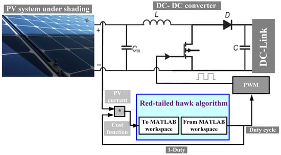
Figure 5. Schematic diagram for PV system with MPPT (* is the product).

Table 1. Specifications of the PV-BES.

Characteristics	Values
$P_{MPP}$	200 W
$I_{MPP}$	7.61 A
$V_{MPP}$	26.3 V
Number of arrays	5
Number of series modules in the array	5
Number of strings in the array	3
DC link voltage	480 V

The duty cycle (d) of the DC boost converter regulates the PV voltage and, consequently, the PV power. It can be represented by the following relation:

$$V_{DC-link}=\frac{1}{1-d}\times V_{PV}$$

(11)

where $V_{pv}$ and $V_{DC-link}$ denote the voltage of the system PV and voltage of the DC link, respectively.

Therefore, the PV voltage can be expressed in terms of the voltage of the DC link as follows:

$$V_{PV}=V_{DC-link}(1-d)$$

(12)

Based on the previous equation, with a constant BES voltage, the PV voltage directly depends on the value (1 − d). Consequently, instead of using a sensor to measure the PV voltage, the value of (1 − d) may be used. Accordingly, the objective needed to be maximized is formulated as follows:

$$f(d)=I_{PV}\times \left(1-d\right) \mathrm{subjected}\hspace{0.17em}\mathrm{to} 0\le d\le 1$$

(13)

where I_pv presents the output current of the PV. The duty cycle is designated to be the outcomes parameter throughout the optimization procedure.

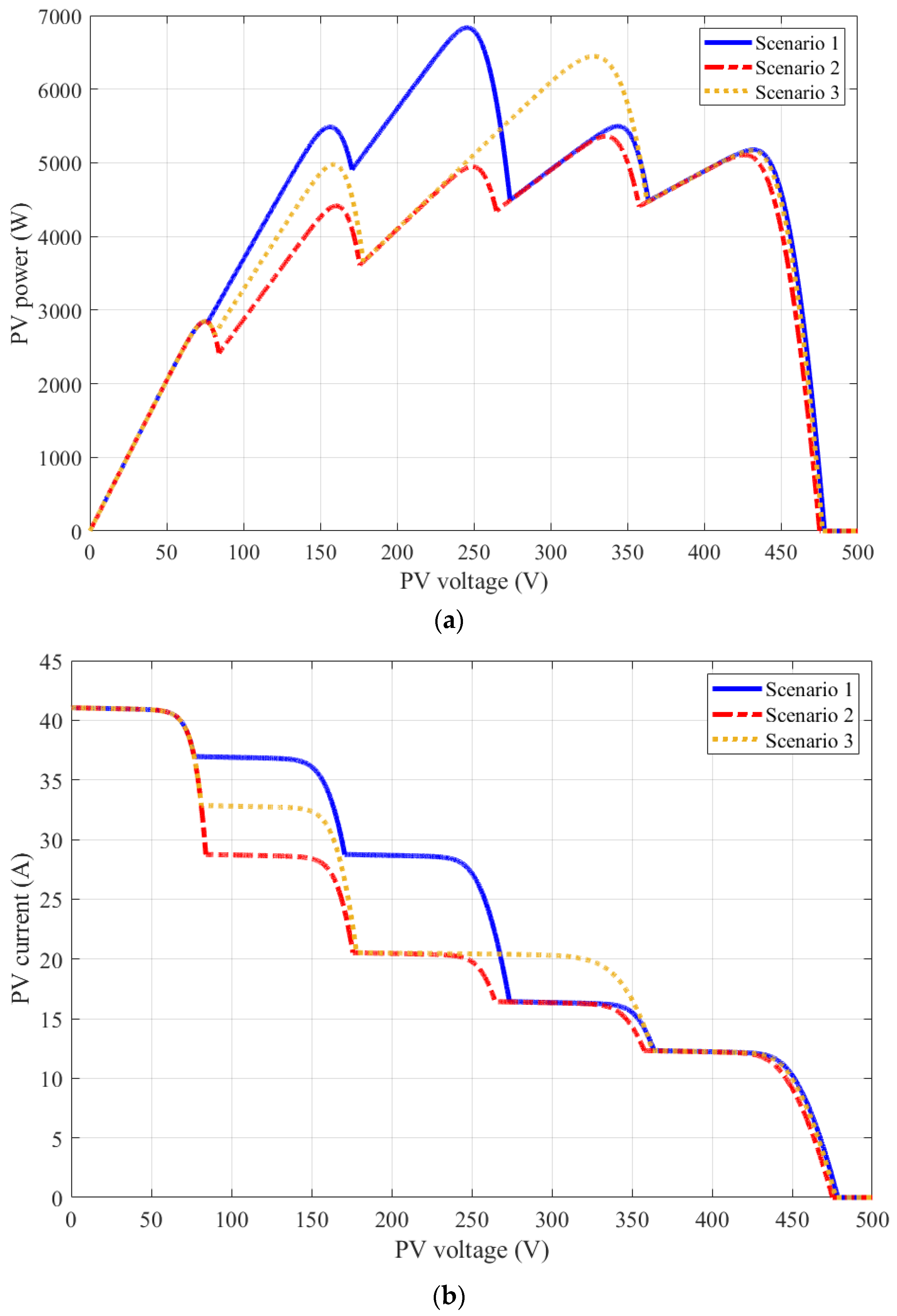
To evaluate the performance of global MPPT based on the RTH, three shading patterns are taken into consideration. Figure 6 and Table 2 show the voltage, power, and current graphs under the considered shading patterns. Changing the shading pattern is considered to vary the position of the global MPP to evaluate the reliability of the proposed global MPPT based on the RTH.

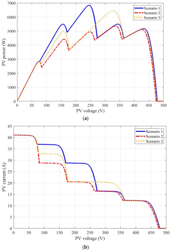
Figure 6. The details of shading scenarios: (a) power against voltage characteristics, and (b) current against voltage characteristics.

Table 2. Shadow structure and data requirements at MPP.

Solar Irradiation (W/m2) of Five Series-Connected PV Systems						Data at MPP
Shading	Array 1	Array 2	Array 3	Array 4	Array 5	Power (W)	Voltage (V)	Current (A)	Duty
First scenario	1000	900	700	400	300	6836.4	245.73	27.82	0.488
Second scenario	1000	700	500	400	300	5361	336	15.96	0.300
Third scenario	1000	800	500	500	300	6445.9	328.2	19.64	0.316

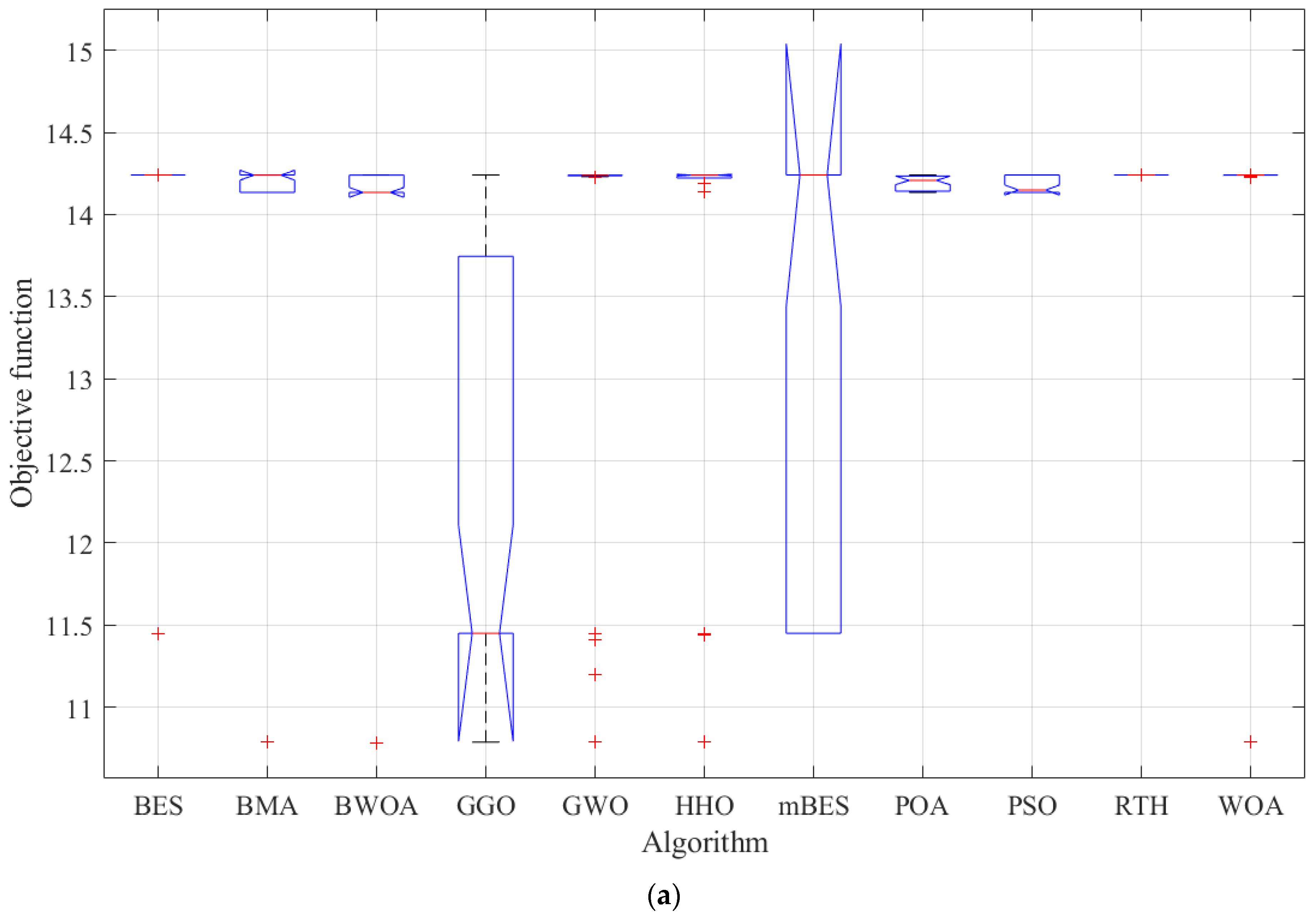
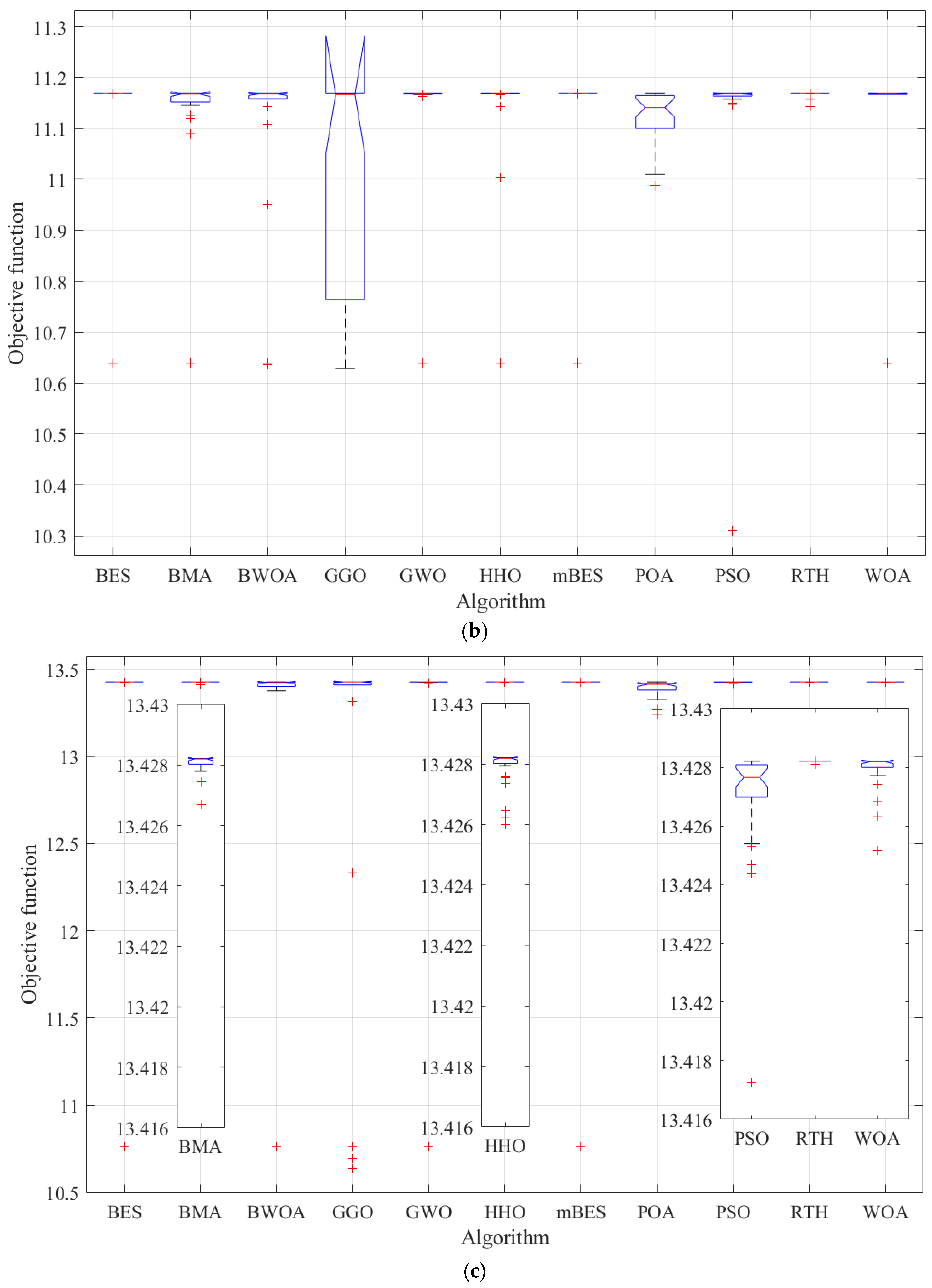
To ensure fairness in the comparison, the total number of communities (5) and repetitions (15) were fixed across all algorithms. Throughout the optimization procedure, the result of the solar power current and (1 − d) was utilized as an indicator of the costs, which was increased. To demonstrate the reliability of the proposed global MPPT based on the RTH, all optimizers were implemented for 30 runs. Table 3 shows the empirical evaluation of the investigated algorithms. The details of the 30 runs for the first, second, and third shading scenarios are presented, respectively, in Table 4, Table 5 and Table 6.

Table 3. Statistical assessments of considered algorithms under different shadow situations.

	BES	BMA	BWOA	GGO	GWO	HHO	mBES	POA	PSO	RTH	WOA
First shading scenario
Best	14.241	14.241	14.241	14.241	14.241	14.241	14.241	14.241	14.241	14.241	14.241
worst	11.45	10.787	10.78	10.787	10.787	10.787	11.45	14.135	14.135	14.241	10.787
mean	13.962	14.089	14.061	12.345	13.835	13.747	13.497	14.195	14.185	14.241	14.125
STD	0.837	0.615	0.611	1.202	1.033	1.093	1.234	0.042	0.052	1.89 × 10−7	0.62
Max. power (W)	6835.63	6835.63	6835.63	6835.63	6835.63	6835.63	6835.63	6835.63	6835.63	6835.63	6835.63
Avg. power (W)	6701.68	6762.85	6749.51	5925.58	6640.86	6598.67	6478.43	6813.42	6808.64	6835.63	6780.03
Efficiency (%)	98.04	98.94	98.74	86.69	97.15	96.53	94.77	99.68	99.61	100	99.19
Second shading scenario
Best	11.168	11.168	11.168	11.168	11.168	11.168	11.168	11.168	11.168	11.168	11.168
worst	10.64	10.639	10.636	10.63	10.64	10.64	10.64	10.988	10.309	11.143	10.64
mean	11.133	11.125	11.086	11.023	11.132	11.091	11.08	11.126	11.137	11.167	11.045
STD	0.132	0.131	0.18	0.225	0.132	0.179	0.197	0.051	0.154	0.005	0.223
Max. power (W)	5360.81	5360.81	5360.81	5360.81	5360.81	5360.81	5360.81	5360.79	5360.81	5360.81	5360.81
Avg. Power (W)	5343.9	5339.97	5321.41	5291.28	5343.58	5323.91	5318.55	5340.45	5345.62	5360.24	5301.56
Efficiency (%)	99.68	99.61	99.27	98.7	99.68	99.31	99.21	99.62	99.72	99.99	98.89
Third shading scenario
Best	13.428	13.428	13.428	13.428	13.428	13.428	13.428	13.428	13.428	13.428	13.428
worst	10.762	13.414	10.762	10.636	10.762	13.426	10.762	13.245	13.417	13.428	13.425
mean	13.339	13.428	13.328	12.935	13.25	13.428	13.25	13.39	13.427	13.428	13.428
STD	0.479	0.003	0.477	1.009	0.665	0.001	0.665	0.049	0.002	2.12 × 10−5	0.001
Max. power (W)	6445.54	6445.54	6445.53	6445.54	6445.54	6445.54	6445.54	6445.53	6445.54	6445.54	6445.54
Avg. Power (W)	6402.88	6445.24	6397.27	6208.9	6359.95	6445.4	6360.22	6427.14	6444.96	6445.54	6445.39
Efficiency (%)	99.34	100	99.25	96.33	98.67	100	98.68	99.71	99.99	100	100

Table 4. Cost function values during first shadow situation.

	BES	BMA	BWOA	GGO	GWO	HHO	mBES	POA	PSO	RTH	WOA
1	14.241	14.238	14.241	11.45	14.241	14.24	14.241	14.159	14.241	14.241	14.241
2	14.241	14.241	14.241	11.45	14.241	11.45	14.241	14.135	14.135	14.241	14.241
3	14.241	14.135	14.241	14.241	14.241	11.441	14.241	14.208	14.135	14.241	14.241
4	11.45	14.241	14.135	13.746	14.241	14.241	11.45	14.225	14.241	14.241	14.241
5	14.241	14.223	14.135	11.45	14.239	14.241	11.45	14.2	14.135	14.241	14.241
6	14.241	14.239	14.135	11.45	14.24	14.239	14.241	14.238	14.241	14.241	14.24
7	14.241	14.135	14.239	11.45	14.241	11.45	14.241	14.183	14.241	14.241	14.241
8	14.241	14.241	14.135	11.45	14.241	14.241	11.45	14.172	14.135	14.241	14.241
9	14.241	14.241	14.241	14.241	14.239	14.241	14.241	14.241	14.241	14.241	14.24
10	14.241	14.135	14.241	11.45	14.239	14.24	11.45	14.135	14.225	14.241	14.237
11	14.241	14.241	14.24	12.85	14.24	14.241	14.241	14.22	14.239	14.241	14.241
12	14.241	10.787	14.241	11.45	14.24	14.24	11.45	14.241	14.135	14.241	14.241
13	14.241	14.135	14.237	11.45	11.45	14.138	14.241	14.22	14.135	14.241	14.24
14	14.241	14.135	14.135	11.45	14.236	14.241	14.241	14.212	14.135	14.241	14.24
15	14.241	14.241	14.241	14.24	14.237	14.241	11.45	14.235	14.241	14.241	14.241
16	14.241	14.241	14.135	14.01	11.413	14.241	14.241	14.135	14.164	14.241	14.241
17	14.241	14.135	14.135	11.661	14.24	14.189	14.241	14.24	14.135	14.241	14.241
18	14.241	14.241	14.135	11.45	10.787	14.239	14.241	14.208	14.24	14.241	14.228
19	14.241	14.135	14.235	13.591	14.224	14.239	14.241	14.135	14.241	14.241	14.241
20	14.241	14.135	14.135	10.787	14.24	14.241	11.45	14.233	14.135	14.241	14.241
21	11.45	14.241	14.135	13.8	14.24	14.241	14.241	14.135	14.241	14.241	14.241
22	14.241	14.241	14.135	13.416	14.231	14.241	14.241	14.135	14.135	14.241	10.787
23	14.241	14.241	14.135	11.45	14.24	14.24	14.241	14.208	14.135	14.241	14.241
24	14.241	14.241	14.135	11.45	14.241	14.241	11.45	14.237	14.135	14.241	14.241
25	14.241	14.148	14.135	14.241	14.237	11.45	14.241	14.24	14.241	14.241	14.241
26	14.241	14.185	14.135	11.445	14.238	14.241	14.241	14.16	14.135	14.241	14.241
27	14.241	14.241	14.135	14.184	11.2	10.787	14.241	14.135	14.24	14.241	14.241
28	14.241	14.241	14.135	12.143	14.239	14.241	14.241	14.231	14.135	14.241	14.241
29	14.241	14.166	10.78	11.45	14.236	14.24	14.241	14.241	14.241	14.241	14.241
30	11.45	14.241	14.135	11.45	14.24	14.223	14.241	14.142	14.135	14.241	14.241

Table 5. Cost function values during second shadow situation.

	BES	BMA	BWOA	GGO	GWO	HHO	mBES	POA	PSO	RTH	WOA
1	11.168	11.168	11.16	11.168	11.168	11.143	11.168	11.168	11.168	11.168	11.168
2	11.168	10.64	10.64	11.168	11.166	11.168	11.168	11.168	11.168	11.168	11.168
3	11.168	11.168	11.168	10.644	11.168	11.168	11.168	10.988	10.309	11.168	10.64
4	11.168	11.166	11.165	11.168	11.168	11.168	11.168	11.143	11.167	11.168	11.167
5	11.168	11.168	11.168	11.034	11.168	11.168	11.168	11.165	11.168	11.143	11.168
6	11.168	11.166	11.168	11.168	10.64	11.168	11.168	11.168	11.167	11.168	11.168
7	11.168	11.168	11.143	11.168	11.168	11.004	11.168	11.168	11.168	11.168	11.168
8	11.168	10.639	11.159	11.162	11.168	11.168	11.168	11.057	11.168	11.168	10.64
9	11.168	11.168	11.168	10.63	11.168	11.168	11.168	11.129	11.166	11.168	11.168
10	11.168	11.168	10.64	11.168	11.168	11.168	11.168	11.011	11.161	11.168	10.64
11	11.168	11.168	11.168	11.168	11.167	11.168	10.64	11.08	11.159	11.168	10.64
12	11.168	11.119	11.168	11.168	11.168	11.168	11.168	11.095	11.168	11.168	11.167
13	11.168	11.168	11.168	11.168	11.168	11.168	11.168	11.168	11.168	11.168	11.168
14	11.168	11.125	11.163	11.158	11.168	11.168	11.168	11.164	11.168	11.158	11.168
15	11.168	11.152	11.166	11.165	10.64	10.64	11.168	11.129	11.167	11.168	11.168
16	10.64	11.151	11.168	10.631	11.168	11.168	11.168	11.097	11.168	11.168	11.168
17	11.168	11.166	11.168	11.168	11.168	11.168	11.168	11.138	11.146	11.168	10.64
18	10.64	11.145	11.168	11.168	11.166	11.168	11.168	11.1	11.168	11.168	11.168
19	11.168	11.165	11.16	10.64	11.166	11.168	11.168	11.139	11.168	11.168	11.167
20	11.168	11.166	11.168	11.157	11.162	11.168	11.168	11.106	11.158	11.168	11.168
21	11.168	11.168	10.951	11.168	11.168	10.64	10.64	11.167	11.164	11.168	11.168
22	11.168	11.168	11.168	11.148	11.168	11.168	11.168	11.129	11.168	11.168	11.168
23	11.168	11.089	11.168	10.765	11.168	10.64	10.64	11.164	11.164	11.168	11.168
24	11.168	11.168	11.168	11.127	11.168	11.168	11.168	11.134	11.163	11.168	11.168
25	11.168	11.167	11.168	10.64	11.168	11.166	11.168	11.01	11.15	11.168	11.168
26	11.168	11.168	10.64	10.64	11.168	11.168	10.64	11.149	11.168	11.168	10.64
27	11.168	11.168	11.108	10.64	11.168	11.168	11.168	11.164	11.168	11.168	11.168
28	11.168	11.168	11.168	11.168	11.168	10.64	11.168	11.158	11.168	11.168	11.168
29	11.168	11.168	10.636	11.168	11.168	11.168	10.64	11.167	11.168	11.168	10.64
30	11.168	11.168	11.167	11.168	11.168	11.168	11.168	11.156	11.168	11.168	11.168

Table 6. Cost function values during third shadow scenario.

	BES	BMA	BWOA	GGO	GWO	HHO	mBES	POA	PSO	RTH	WOA
1	13.428	13.428	13.395	13.426	13.428	13.428	13.428	13.426	13.428	13.428	13.428
2	13.428	13.428	13.377	13.427	13.428	13.428	13.428	13.269	13.428	13.428	13.428
3	13.428	13.428	13.427	13.428	13.428	13.426	13.428	13.354	13.428	13.428	13.428
4	13.428	13.428	13.402	13.412	13.428	13.428	13.428	13.418	13.428	13.428	13.428
5	13.428	13.428	13.428	10.636	13.426	13.428	13.428	13.428	13.427	13.428	13.428
6	13.428	13.428	13.425	10.762	13.428	13.428	13.428	13.417	13.425	13.428	13.428
7	13.428	13.428	13.427	13.428	10.762	13.428	13.428	13.407	13.424	13.428	13.428
8	13.428	13.428	13.428	13.428	13.428	13.428	10.762	13.406	13.417	13.428	13.428
9	13.428	13.428	13.427	13.428	13.428	13.428	13.428	13.326	13.428	13.428	13.426
10	13.428	13.428	13.428	13.428	13.428	13.428	13.428	13.386	13.428	13.428	13.427
11	13.428	13.428	13.424	13.428	13.428	13.428	13.428	13.417	13.427	13.428	13.428
12	10.762	13.428	13.425	10.762	13.428	13.426	13.428	13.418	13.428	13.428	13.428
13	13.428	13.428	13.425	13.418	13.428	13.428	13.428	13.355	13.425	13.428	13.428
14	13.428	13.428	13.423	13.427	13.428	13.428	13.428	13.422	13.426	13.428	13.428
15	13.428	13.428	13.426	13.428	13.428	13.428	13.428	13.4	13.427	13.428	13.428
16	13.428	13.428	13.428	13.427	13.427	13.428	13.428	13.421	13.428	13.428	13.428
17	13.428	13.428	13.377	13.411	13.428	13.428	13.428	13.423	13.428	13.428	13.428
18	13.428	13.428	13.378	13.428	13.426	13.427	13.428	13.412	13.428	13.428	13.428
19	13.428	13.428	13.423	13.314	13.427	13.428	13.428	13.245	13.428	13.428	13.428
20	13.428	13.428	13.425	13.428	13.428	13.428	13.428	13.417	13.428	13.428	13.428
21	13.428	13.428	13.418	13.428	13.423	13.428	13.428	13.417	13.428	13.428	13.425
22	13.428	13.414	13.419	10.695	13.428	13.426	10.762	13.417	13.428	13.428	13.428
23	13.428	13.428	13.4	13.428	13.428	13.428	13.428	13.363	13.425	13.428	13.428
24	13.428	13.428	13.383	13.428	13.426	13.428	13.428	13.428	13.427	13.428	13.428
25	13.428	13.428	13.421	13.428	13.427	13.428	13.428	13.399	13.428	13.428	13.428
26	13.428	13.427	13.428	12.333	13.428	13.428	13.428	13.405	13.427	13.428	13.427
27	13.428	13.428	13.428	13.428	10.762	13.428	13.428	13.271	13.428	13.428	13.428
28	13.428	13.428	13.428	13.428	13.428	13.428	13.428	13.381	13.428	13.428	13.428
29	13.428	13.428	10.762	10.762	13.427	13.428	13.428	13.428	13.428	13.428	13.428
30	13.428	13.427	13.426	13.421	13.428	13.428	13.428	13.418	13.427	13.428	13.428

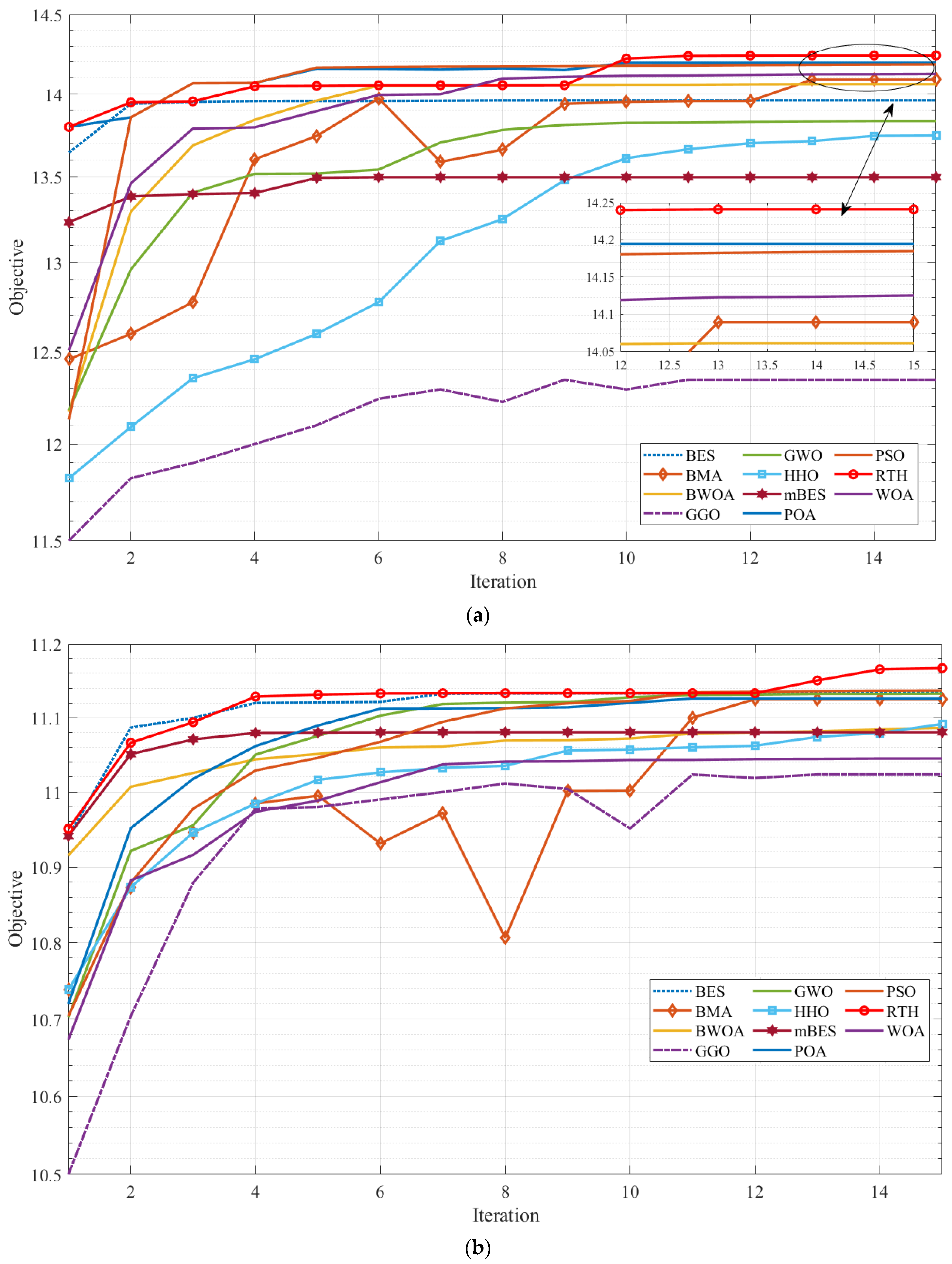
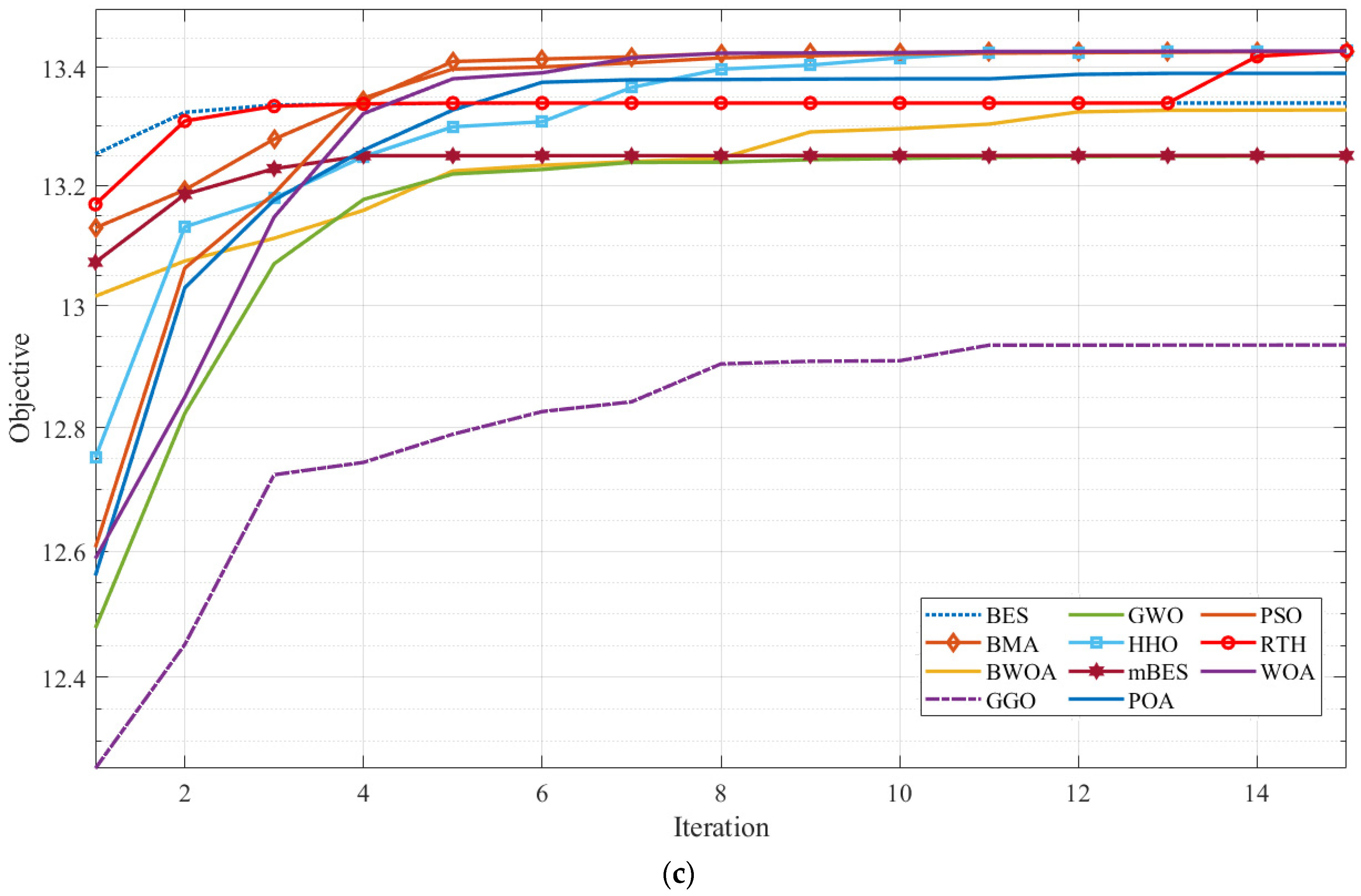
Considering Table 3, the proposed global MPPT based on the RTH has the highest performance compared with other optimizers. For the first shading situation, the mean PV power values varied between 6835.63 W and 5925.58 W. The RTH reaches the highest PV power of 6835.63 W flowing through PSO (6808.64 W). GGO achieved the smallest PV power production of 5925.58 W. The STD numbers range from 1.89 × 10⁻⁷ to 1.234. The RTH has the smallest STD at 1.89 × 10⁻⁷, followed by the POA with the lowest (0.042). The worst value of the STD of 1.234 is obtained by mBES. In the second shading situation, the mean PV power levels varied between 5360.24 W to 5291.28 W. The RTH achieves the maximum PV power of 5360.24 W, followed by PSO (5345.62 W), whereas the minimum PV power of 5291.28 W is obtained by GGO. The STD values varied between 0.005 and 0.225. The RTH has the lowest STD of 0.005, after the POA (0.051). GGO obtains an unacceptable STD of 0.225. For the third shading circumstance, the average PV power output varied from 6445.54 W to 6208.9 W. The RTH generates the highest solar energy output of 6445.54 W, which is followed by the WOA (6445.39 W), while GGO has the lowest PV power of 6208.9 W. The STD values varied between 2.12 × 10⁻⁵ and 1.009, while the minimum STD of 2.12 × 10⁻⁵ is reached by the RTH, followed by the WOA (0.001), with GGO achieving the lowest STD score of 1.009. Figure 7 depicts the fluctuation in the average cost function during the optimization phase for the three shading schemes. Figure 8 shows the dynamic response of the PV system using the RTH under different scenarios.

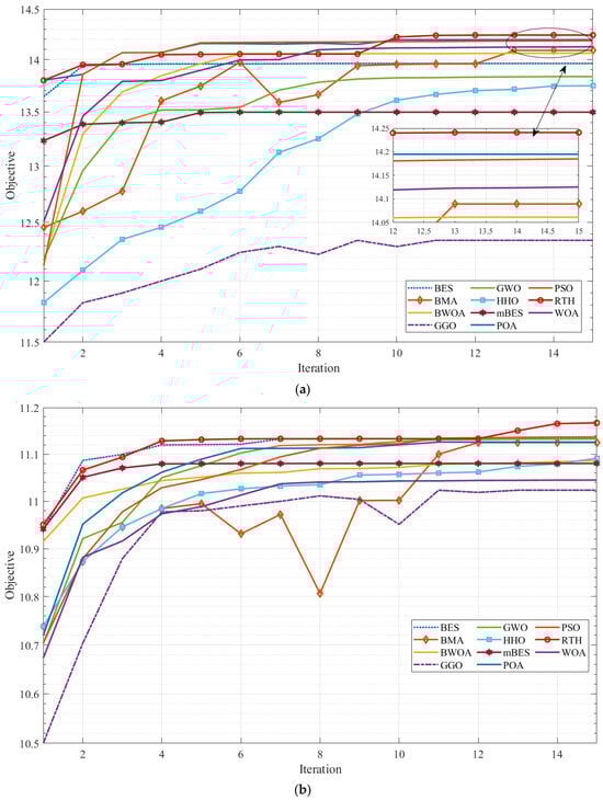
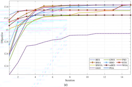
Figure 7. Mean objective values: (a) first shadow scenario, (b) second shadow scenario, and (c) third shadow scenario.

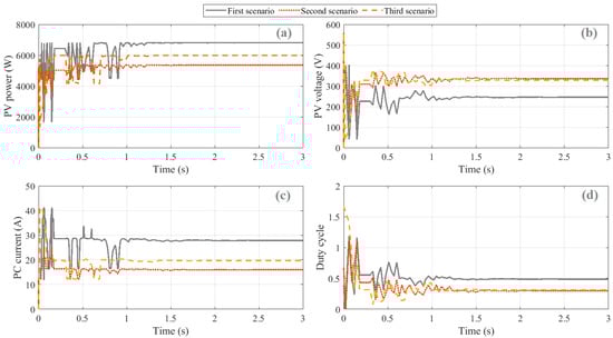
Figure 8. Dynamic response of PV system using RTH: (a) PV power, (b) PV voltage, (c) PV current, and (d) duty cycle.

Table 7 presents a comprehensive analytical study using the ANOVA test to assess the performance of each optimizer. In this test, DF represents the degree of freedom, SS represents the sum of squares, MS represents the mean squared error (=DF/SS), F represents the ratio of the mean squared errors, and P represents the likelihood that the calculated test statistic can assume a value greater than the test statistic itself. The P value is considerably less than the F value for each case, indicating that the column values, which comprise the mean values, are substantially distinct. Simultaneously, Figure 9 provides a visual depiction of the rankings, thereby validating the RTH algorithm with remarkable stability and precision.

Table 7. ANOVA results considering different shading scenarios.

	Source	DF	SS	MS	F	P
1st scenario	Columns	10	89.221	8.92212	13.42	1.12 × 10−19
	Error	319	212.104	0.6649
	Total	329	301.325
2nd scenario	Columns	10	0.55924	0.05592	2.11	0.0235
	Error	319	8.46175	0.02653
	Total	329	9.02099
3rd scenario	Columns	10	6.6007	0.66007	2.97	0.0014
	Error	319	70.8151	0.22199
	Total	329	77.4159

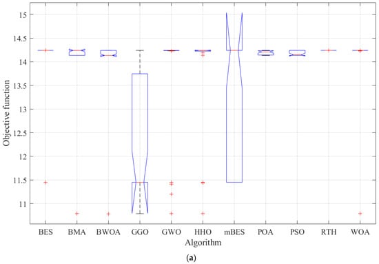
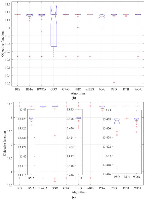
Figure 9. ANOVA ranking: (a) first shadow scenario, (b) second shadow scenario, and (c) third shadow scenario.

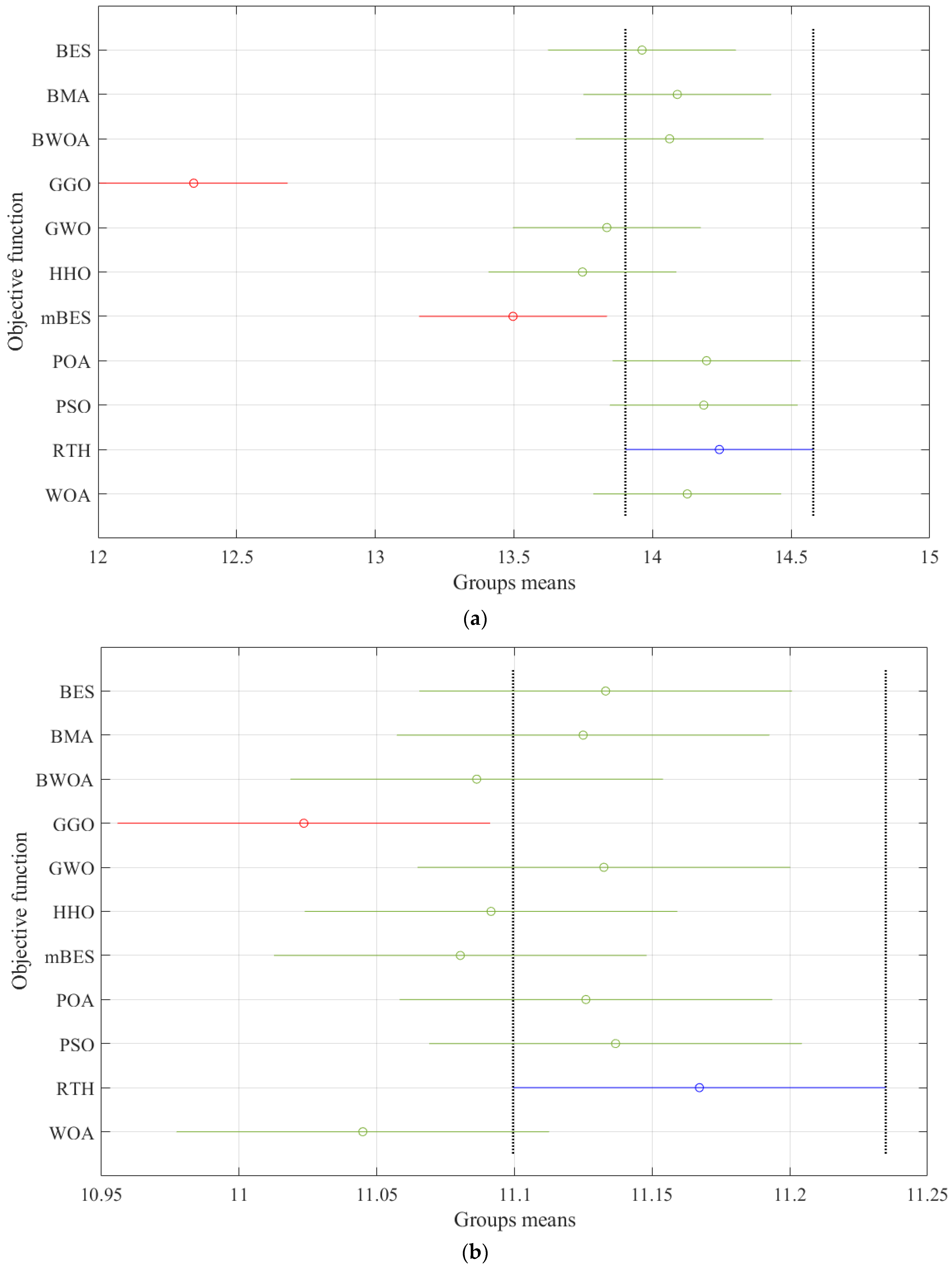
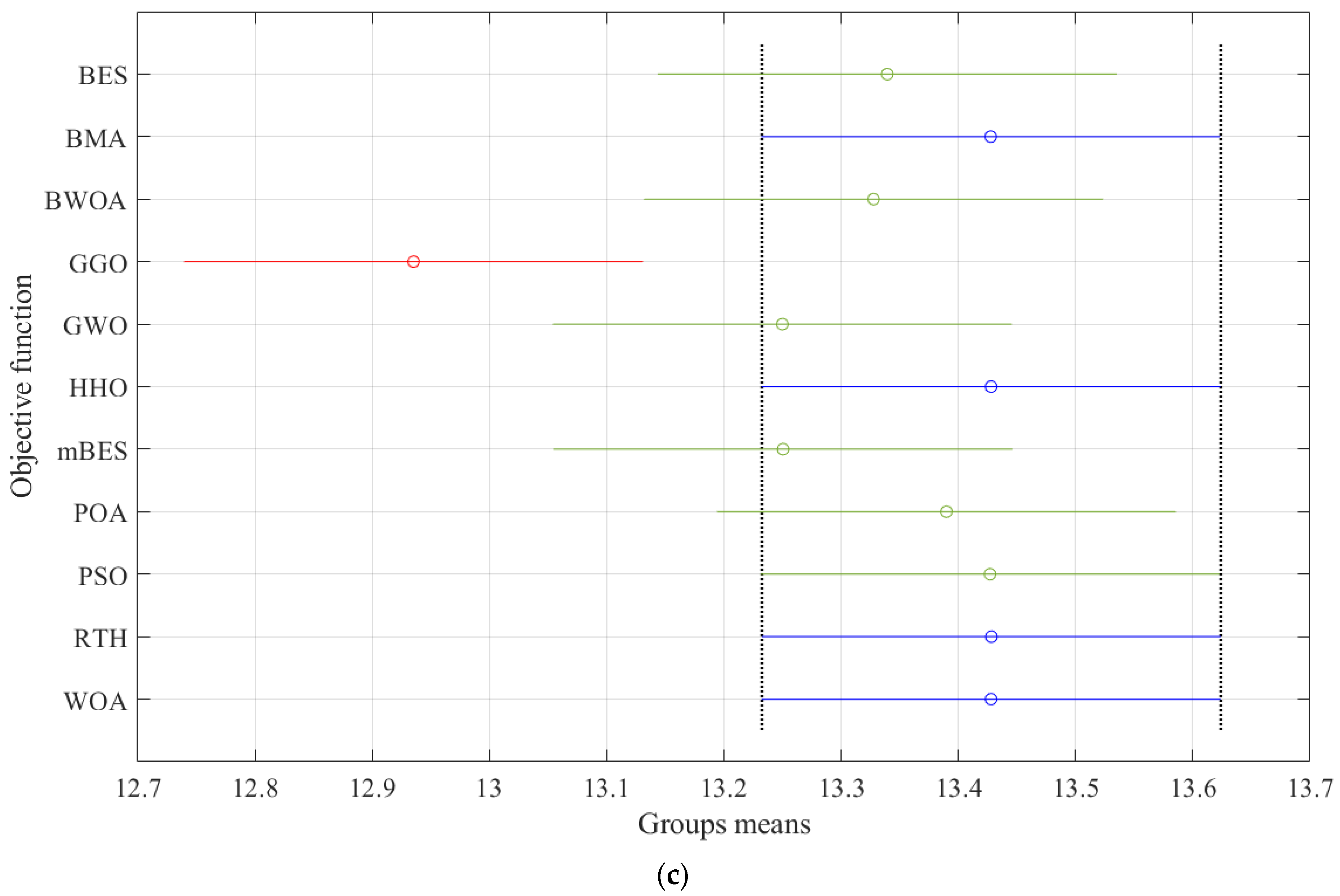
To back up the ANOVA findings, a Tukey Honest Significant Difference (Tukey HSD) post hoc evaluation was carried out. Figure 10 illustrates the results for the first, second, and third shading situations. The RTH has the greatest meaning compared with other algorithms. As demonstrated in Figure 10a, for the first shading scenarios, the lowest performance is obtained by GGO and mBES. For the second shading scenarios as shown in Figure 10b, the lowest performance is also obtained by GGO.

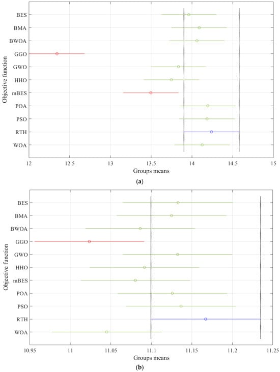
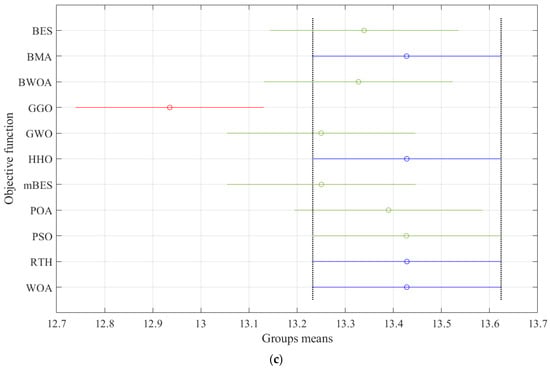
Figure 10. Tukey test: (a) first shadow scenario, (b) second shadow scenario, and (c) third shadow scenario.

5. Conclusions

To extract the global PV power under shading, most global MPPT methods in the literature require current and voltage sensors, as well as solar irradiance and/or temperature sensors at the PV array side. Reducing the number of sensors is crucial for reliability and cost savings. This paper proposes a single-sensor global MPPT based on the recent red-tailed hawk (RTH) algorithm. To prove the superiority of the RTH, the results are compared with another ten algorithms. Three shading scenarios are considered for changing the location of the global MPP to test the reliability of the RTH. As an example, for the first shading situation, the average PV power values ranged between 6835.63 W and 5925.58 W. The RTH achieves the maximum PV power of 6835.63 W flowing through PSO (6808.64 W). The lowest PV power of 5925.58 W is obtained by GGO. The STD values vary between 1.89 × 10⁻⁷ and 1.234. The lowest STD of 1.89 × 10⁻⁷ is achieved by the RTH followed by the POA (0.042). The worst value of the STD of 1.234 is obtained by mBES. In sum, the results verified the effectiveness of the suggested global MPPT based on the RTH in precisely capturing the global MPP compared with other methods. In future work, the RTH will be evaluated for the first time by a new application related to wind energy; in addition, the experimental validation of the current finding will be considered.

References

- Osman, A.I.; Chen, L.; Yang, M.; Msigwa, G.; Farghali, M.; Fawzy, S.; Rooney, D.W.; Yap, P.-S. Cost, environmental impact, and resilience of renewable energy under a changing climate: A review. Environ. Chem. Lett. 2023, 21, 741–764. [Google Scholar] [CrossRef]
- Holechek, J.L.; Geli, H.M.E.; Sawalhah, M.N.; Valdez, R. A global assessment: Can renewable energy replace fossil fuels by 2050? Sustainability 2022, 14, 4792. [Google Scholar] [CrossRef]
- Kadrić, D.; Aganović, A.; Kadrić, E. Multi-objective optimization of energy-efficient retrofitting strategies for single-family residential homes: Minimizing energy consumption, CO2 emissions and retrofit costs. Energy Rep. 2023, 10, 1968–1981. [Google Scholar] [CrossRef]
- Han, J.-Y.; Li, S.-Y. Impact of temperature and solar irradiance in shadow covering scenarios via two-way sensitivity analysis for rooftop solar photovoltaics. Energy Sources Part A Recovery Util. Environ. Eff. 2024, 46, 3165–3176. [Google Scholar] [CrossRef]
- Sharma, D.; Jalil, M.F.; Ansari, M.S.; Bansal, R.C. A review of PV array reconfiguration techniques for maximum power extraction under partial shading conditions. Optik 2023, 275, 170559. [Google Scholar] [CrossRef]
- Alblawi, A.; Said, T.; Talaat, M.; Elkholy, M.H. PV solar power forecasting based on hybrid MFFNN-ALO. In Proceedings of the 2022 13th International Conference on Electrical Engineering (ICEENG), Cairo, Egypt, 29–31 March 2022; pp. 52–56. [Google Scholar]
- Elkholy, M.H.; Elymany, M.; Ueda, S.; Halidou, I.T.; Fedayi, H.; Senjyu, T. Maximizing microgrid resilience: A two-stage AI-Enhanced system with an integrated backup system using a novel hybrid optimization algorithm. J. Clean. Prod. 2024, 446, 141281. [Google Scholar] [CrossRef]
- Premkumar, M.; Kumar, C.; Anbarasan, A.; Sowmya, R. A new maximum power point tracking technique based on whale optimisation algorithm for solar photovoltaic systems. Int. J. Ambient Energy 2022, 43, 5627–5637. [Google Scholar] [CrossRef]
- Premkumar, M.; Sowmya, R. An effective maximum power point tracker for partially shaded solar photovoltaic systems. Energy Rep. 2019, 5, 1445–1462. [Google Scholar] [CrossRef]
- Korany, E.; Yousri, D.; Attia, H.A.; Zobaa, A.F.; Allam, D. A novel optimized dynamic fractional-order MPPT controller using hunter pray optimizer for alleviating the tracking oscillation with changing environmental conditions. Energy Rep. 2023, 10, 1819–1832. [Google Scholar] [CrossRef]
- Fathy, A.; Amer, D.A.; Al-Dhaifallah, M. Modified tunicate swarm algorithm-based methodology for enhancing the operation of partially shaded photovoltaic system. Alex. Eng. J. 2023, 79, 449–470. [Google Scholar] [CrossRef]
- Eltamaly, A.M. A novel benchmark shading pattern for PV maximum power point trackers evaluation. Sol. Energy 2023, 263, 111897. [Google Scholar] [CrossRef]
- Eltamaly, A.M. A novel musical chairs algorithm applied for MPPT of PV systems. Renew. Sustain. Energy Rev. 2021, 146, 111135. [Google Scholar] [CrossRef]
- Nguyen, T.B.N.; Chao, K.-H. Fast Maximum Power Tracking for Photovoltaic Module Array Using Only Voltage and Current Sensors. Sens. Mater. 2023, 35, 2619–2635. [Google Scholar]
- Silvestre, S.; Boronat, A.; Chouder, A. Study of bypass diodes configuration on PV modules. Appl. Energy 2009, 86, 1632–1640. [Google Scholar] [CrossRef]
- Celikel, R. A global MPPT technique for PV systems under partial shading conditions. Int. J. Electron. 2023, 111, 1163–1178. [Google Scholar] [CrossRef]
- Silaa, M.Y.; Barambones, O.; Bencherif, A.; Rahmani, A. A New MPPT-Based Extended Grey Wolf Optimizer for Stand-Alone PV System: A Performance Evaluation versus Four Smart MPPT Techniques in Diverse Scenarios. Inventions 2023, 8, 142. [Google Scholar] [CrossRef]
- Qi, P.; Xia, H.; Cai, X.; Yu, M.; Jiang, N.; Dai, Y. Novel Global MPPT Technique Based on Hybrid Cuckoo Search and Artificial Bee Colony under Partial-Shading Conditions. Electronics 2024, 13, 1337. [Google Scholar] [CrossRef]
- Fathy, A.; Rezk, H. A novel methodology for simulating maximum power point trackers using mine blast optimization and teaching learning based optimization algorithms for partially shaded photovoltaic system. J. Renew. Sustain. Energy 2016, 8, 023503. [Google Scholar] [CrossRef]
- Rezk, H.; Fathy, A. Simulation of global MPPT based on teaching–learning-based optimization technique for partially shaded PV system. Electr. Eng. 2017, 99, 847–859. [Google Scholar] [CrossRef]
- Das, S.K.; Verma, D.; Nema, S.; Nema, R.K. Shading mitigation techniques: State-of-the-art in photovoltaic applications. Renew. Sustain. Energy Rev. 2017, 78, 369–390. [Google Scholar] [CrossRef]
- Ko, S.W.; Ju, Y.C.; Hwang, H.M.; So, J.H.; Jung, Y.-S.; Song, H.-J.; Song, H.-E.; Kim, S.-H.; Kang, G.H. Electric and thermal characteristics of photovoltaic modules under partial shading and with a damaged bypass diode. Energy 2017, 128, 232–243. [Google Scholar] [CrossRef]
- Pannebakker, B.B.; de Waal, A.C.; van Sark, W.G.J.H.M. Photovoltaics in the shade: One bypass diode per solar cell revisited. Prog. Photovolt. Res. Appl. 2017, 25, 836–849. [Google Scholar] [CrossRef]
- Ferahtia, S.; Houari, A.; Rezk, H.; Djerioui, A.; Machmoum, M.; Motahhir, S.; Ait-Ahmed, M. Red-tailed hawk algorithm for numerical optimization and real-world problems. Sci. Rep. 2023, 13, 12950. [Google Scholar] [CrossRef] [PubMed]
Disclaimer/Publisher’s Note: The statements, opinions and data contained in all publications are solely those of the individual author(s) and contributor(s) and not of MDPI and/or the editor(s). MDPI and/or the editor(s) disclaim responsibility for any injury to people or property resulting from any ideas, methods, instructions or products referred to in the content. |
© 2024 by the authors. Licensee MDPI, Basel, Switzerland. This article is an open access article distributed under the terms and conditions of the Creative Commons Attribution (CC BY) license (https://creativecommons.org/licenses/by/4.0/).