A Data-Driven Method for Calculating Neutron Flux Distribution Based on Deep Learning and the Discrete Ordinates Method

Abstract

The efficient and accurate calculation of neutron flux distribution is essential for evaluating the safety of nuclear facilities and the surrounding environment. While traditional numerical simulation methods such as the discrete ordinates (S_N) method and Monte Carlo method have demonstrated excellent performance in terms of accuracy, their complex solving process incurs significant computational costs. This paper explores a data-driven and efficient method for obtaining neutron flux distribution based on deep learning, specifically targeting shielding problems with constant geometry and varying material cross-sections in practical engineering. The proposed method bypasses the intricate numerical transport calculation process of the discrete ordinates method by constructing a surrogate model that captures the correlation between transport characteristics and neutron flux from data characteristics. Simulations were carried out using Kobayashi-1 and Kobayashi-2 geometric models for shielding problems with constant geometry and varying material cross-sections. A series of validations have proved that the data-driven surrogate model demonstrates high generalization ability and reliability, while reducing the time required to obtain neutron flux distribution to 0.1 s without compromising on calculation accuracy compared to the discrete ordinates method.

1. Introduction

The neutron flux is a measure of the rate of neutron flow through a unit area, and it is the key physical quantity in radiation shielding calculations. It provides key information for ensuring environmental safety in radiation. Therefore, the efficient and accurate calculation of this value is the primary goal of shielding calculations [1]. In practical engineering, in order to judge whether the radiation field is within the safe radiation dose range, it is necessary to monitor the complex three-dimensional radiation field in real time, which requires the method for calculating the neutron flux distribution not only to adapt to the dynamic conditions of the radiation field, but also to have the ability to quickly calculate large geometrically complex problems. However, the traditional numerical calculation methods are unable to reconcile the demands of computational efficiency with those of accuracy.

Currently, the commonly used methods [2,3] for solving the neutron flux distribution in the shielding calculations are the discrete ordinates method and the Monte Carlo method. To solve the transport equation by the discrete ordinates method, the transport equation must be discretized with multiple variables and coupled equations must be established. The scale and complexity of the coupled equations increase with the complexity of the shielding structure and scale, and the solution efficiency is directly affected. In order to improve the computational efficiency of the discrete ordinates method, many different methods have been studied. The iterative optimization method enhances computational efficiency by optimizing the solution process [4]. GPU acceleration [5] and CPU parallel acceleration [6,7,8] leverage advanced computing resources and high-performance computer hardware to expedite the solution speed, thereby improving transport computing efficiency. The adaptive method [9,10,11,12,13,14] reduces the scale of transport equations based on estimated local errors in order to save time. The multi-level tree grid [15,16] utilizes coarse grids to represent problem areas that do not require fine grids, thus reducing the scale of transport equations and alleviating solving pressure. The Monte Carlo method uses the continuous energy point cross-sections to simulate the calculation, and the statistical error can be obtained directly. The whole process of particles from appearance to disappearance can be simulated in the discrete system, and it has strong geometric adaptability. Using the Monte Carlo method to simulate large complex reactors means that as the particle simulation scale increases, the particle simulation process slows down and computational efficiency decreases. Furthermore, Stochastic Differential Equations (SDEs) are an appropriate mathematical tool for modelling transport equations, and their results are in close agreement with Monte Carlo calculations. E. J. Allen derived the Stochastic Differential Equation and the Stochastic Partial Differential Equation for the neutron angular flux with time in general three-dimensional media [17], and compared the numerical solution of the stochastic differential equation with the Monte Carlo calculation of an independent formula to ensure the accuracy of the derivation. Hajas T established a connection between the Dynamic Monte Carlo (DMC) method and differential equation formalism [18]. A Non-Analog Monte Carlo (NAMC) model of the Stochastic Point-Kinetics equation (SPKe) is developed to determine a noise model that can effectively approximate the DMC locus.

The discrete ordinates method and Monte Carlo method have boundary dependence and need to set appropriate boundary conditions to complete calculation. As a highly parallel information processing system, the neural network possesses robust adaptive learning capabilities and is capable of managing complex nonlinear systems with multiple inputs and outputs [19,20]. The neural network learns the complex relationship between inputs and outputs from rich data, and summarizes the approximate function that can describe the relationship between inputs and outputs. The trained neural network can effectively determine the output target physical quantity based on the input, making it suitable for binary classification, multi-classification, and mathematical regression problems. With the continuous exploration and improvement of neural network functions and the continuous improvement of computer performance, many studies have focused on the intersectant and syncretic of neural networks and neutron flux. Zhou W studied a radiation field reconstruction method based on BP neural networks [21]. The accuracy of the reconstructed radiation field is improved by learning rate adaptive attenuation and multiple sampling methods. Li Z et al. used a deep neural network to calculate the cross-sections, taking into account the complex nonlinear relationship between the reactor variables [22]. Zhu O discussed the superiority of the artificial neural network method in neutron spectrum expansion by comparing it with the maximum entropy expansion method [23]. Cao C proposed a “two-step” neutron spectrum unwrapping method based on artificial neural networks to improve the computational efficiency of online wide-range neutron spectrum unwrapping technology [24]. Dos Santos demonstrated the performance of the Deep Rectifier Neural Network (DRNN) in identifying nuclear accidents [25]. Pei C proposed a method to reconstruct the neutron field based on the energy distribution of neural networks [26]. Through transport calculation and reconstruction calculation, the neutron field inside the reactor pressure vessel and in the core region is reconstructed by using the measured data outside the reactor. Song used neural networks to optimize shielding structures for marine reactors [27], and applied the neural network algorithm and the genetic algorithm to optimize the shielding design [28], which is two orders of magnitude faster than the Monte Carlo method. The neural network method is also used in the study of radiation dose [29]. The results of dose computation with the Artificial Neural Network (ANN) are available in less than 2 s. Based on the physics-informed neural network (PINN), Wang J proposed the conservative PINN (cPINN) to solve the neutron diffusion problem in inhomogeneous media, and the proposed BC-imposed method can help to improve the cPINN performance [30]. Overall, the neural network approach allows the neutron flux distribution of the radiation field to be obtained without the need for complex numerical solution methods, and effectively improves the efficiency of obtaining the neutron flux distribution.

In the context of large geometries, both the discrete ordinates and Monte Carlo methods can be time-consuming, taking hours or more to compute the shielding problem. This paper explores the use of deep learning as a potential method for efficiently obtaining neutron flux distribution based on the discrete ordinates method. By incorporating the specific characteristics of changes in shielding structure, the discrete ordinates method is utilized to simulate potential radiation field changes during actual transport. The neutron flux distribution is collected at each instance and used to train a deep learning neural network in order to develop a surrogate model. This model can then be employed to obtain the neutron flux distribution in an efficient manner.

2. Methodology

2.1. Deep Learning Neural Network

Deep learning employs backpropagation algorithms to identify intricate structures within expansive datasets [31]. Deep learning is a machine learning method based on neural networks that learns input data layer by layer through multi-layer neural networks, thereby enabling the modelling of complex nonlinear relationships. The basic structure of the neural network is shown in Figure 1. The relationship between input neurons x, y, z and output neuron $\mathrm{u}$ is described by weight ${\mathsf{\omega }}_1,{\mathsf{\omega }}_2,{\mathsf{\omega }}_3$, bias $\mathrm{b}$, and activation function $\mathrm{f}$, as shown:

$$\mathrm{u}=\mathrm{f}(\mathrm{x}{\mathsf{\omega }}_1+\mathrm{y}{\mathsf{\omega }}_2+\mathrm{z}{\mathsf{\omega }}_3+\mathrm{b}),$$

(1)

As the complexity of neural networks increases, their capacity to represent intricate relationships within data improves. The activation function in neural networks plays a crucial role in introducing nonlinearity to the output of neurons, thereby enhancing the neural network’s ability to approximate complex functions. Throughout the training process, the forward loss function calculates the difference between the predicted and actual values. The overall performance is evaluated through the loss function, which aggregates errors across all samples. Utilizing the derivative of the loss function, the optimizer adjusts each weight in the forward calculation along the direction of the minimum gradient. The iterative process continues until the loss function reaches a satisfactory value. The process of training is to improve the capacity of the neural network to approximate complex functions.

However, in practical applications, it is not sufficient for neural networks to demonstrate strong fitting performance; they must also exhibit a certain degree of generalization ability. It is necessary for neural networks to be capable of effectively predicting the output of unknown inputs. The train loss and the test loss are worthy of observation.

2.2. Discrete Ordinates Method Transport Solution

The steady state of neutron transport equation is a linear differential-integral equation with six independent variables, the phase space $(\overrightarrow{\mathrm{r}},\mathrm{E},\overrightarrow{\mathsf{\Omega }})$, containing space $\overrightarrow{\mathrm{r}}(\mathrm{x},\mathrm{y},\mathrm{z})$, energy, and angle $\overrightarrow{\mathsf{\Omega }}(\mathsf{\mu },\mathsf{\eta })$, as shown:

$$\begin{array}{l}\overrightarrow{\mathsf{\Omega }}\cdot \nabla \mathsf{\psi }(\overrightarrow{\mathrm{r}},\mathrm{E},\overrightarrow{\mathsf{\Omega }})+{\mathrm{\Sigma }}_{\mathrm{t}}(\overrightarrow{\mathrm{r}},\mathrm{E})\mathsf{\psi }(\overrightarrow{\mathrm{r}},\mathrm{E},\overrightarrow{\mathsf{\Omega }})\\ ={\displaystyle {\int }_0^{\infty }\mathrm{d}{\mathrm{E}}^{\prime }{\displaystyle {\int }_0^{4\mathrm{\pi }}{\mathrm{\Sigma }}_{\mathrm{s}}(\overrightarrow{\mathrm{r}},{\mathrm{E}}^{\prime }\to \mathrm{E},{\overrightarrow{\mathsf{\Omega }}}^{\prime }\to \overrightarrow{\mathsf{\Omega }})\mathsf{\psi }(\overrightarrow{\mathrm{r}},{\mathrm{E}}^{\prime },\overrightarrow{\mathsf{\Omega }})\mathrm{d}{\overrightarrow{\mathsf{\Omega }}}^{\prime }+\mathrm{q}(\overrightarrow{\mathrm{r}},\mathrm{E},\overrightarrow{\mathsf{\Omega }})}}\end{array}$$

(2)

where $\mathsf{\psi }(\overrightarrow{\mathrm{r}},\mathrm{E},\overrightarrow{\mathsf{\Omega }})$ is the flux, $\mathrm{q}(\overrightarrow{\mathrm{r}},\mathrm{E},\overrightarrow{\mathsf{\Omega }})$ is the fixed source, ${\mathrm{\Sigma }}_{\mathrm{t}}(\overrightarrow{\mathrm{r}},\mathrm{E})$ is the total cross-sections, and ${\mathrm{\Sigma }}_{\mathrm{s}}(\overrightarrow{\mathrm{r}},{\mathrm{E}}^{\prime }\to \mathrm{E},{\overrightarrow{\mathsf{\Omega }}}^{\prime }\to \overrightarrow{\mathsf{\Omega }})$ is the scattering cross-sections. The first term on the right side of the equation is the scattering source. Due to the differential and integral properties of the transport equation, the exact analytical solution of the transport equation can be obtained only in simple problems. Therefore, numerical approximation is often used to solve practical problems. The discrete ordinates method is a deterministic method that requires each variable to be processed discretely. The continuous energy is divided into several appropriate energy groups by the multi-group approximation method. The discrete ordinates method is used to discretize the angle variables. The original continuous direction variable is discretized into M specific discrete directions. The transport equation after angle discretization by the discrete ordinates method is:

$${\mathsf{\Omega }}_{\mathrm{m}}\cdot \nabla {\mathsf{\psi }}_{\mathrm{m}}(\overrightarrow{\mathrm{r}})+{\mathrm{\Sigma }}_{\mathrm{t}}(\overrightarrow{\mathrm{r}}){\mathsf{\psi }}_{\mathrm{m}}(\overrightarrow{\mathrm{r}})={\mathrm{Q}}_{\mathrm{s},\mathrm{m}}(\overrightarrow{\mathrm{r}})+{\mathrm{q}}_{\mathrm{m}}(\overrightarrow{\mathrm{r}}),$$

(3)

where m is the discrete direction number, ${\mathrm{Q}}_{\mathrm{s},\mathrm{m}}$ and ${\mathrm{q}}_{\mathrm{m}}$ are the scattering and fixed source terms, respectively. For spatial variables, the finite difference method [32] or finite element method [33] is used. The discretization method transforms the original transport equation into a large set of equations that can be easily solved. After solving the neutron angular flux of each phase space, the neutron scalar flux and the flux moment in the phase space are calculated by the numerical integral approximation method, as shown:

$${\mathsf{\varphi }}_{\mathrm{n}}^{\mathrm{k}}(\overrightarrow{\mathrm{r}})={\displaystyle \sum _{\mathrm{m}=1}^{\mathrm{M}}{\mathrm{w}}_{\mathrm{m}}{\mathsf{\psi }}_{\mathrm{m}}{\mathrm{Y}}_{\mathrm{n}}^{*\mathrm{k}}({\overrightarrow{\mathsf{\Omega }}}_{\mathrm{m}})},$$

(4)

where ${\mathsf{\varphi }}_{\mathrm{n}}^{\mathrm{k}}(\overrightarrow{\mathrm{r}})$ is the flux moment of order n, k; ${\mathrm{Y}}_{\mathrm{n}}^{*\mathrm{k}}$ is the adjoint spherical harmonic, M is the total number of discrete directions, ${\mathrm{w}}_{\mathrm{m}}$ is the weight coefficient corresponding to the discrete direction m, and the anisotropic scattering source can be approximated by the following formula:

$${\mathrm{Q}}_{\mathrm{s},\mathrm{m}}(\overrightarrow{\mathrm{r}})\approx {\displaystyle \sum _{\mathrm{n}=0}^{\mathrm{N}}\frac{2\mathrm{n}+1}{4\mathrm{\pi }}{\mathrm{\Sigma }}_{\mathrm{s},\mathrm{n}}(\overrightarrow{\mathrm{r}}){\displaystyle \sum _{\mathrm{k}=-\mathrm{n}}^{\mathrm{n}}{\mathsf{\varphi }}_{\mathrm{n}}^{\mathrm{k}}(\overrightarrow{\mathrm{r}}){\mathrm{Y}}_{\mathrm{n}}^{\mathrm{k}}({\overrightarrow{\mathsf{\Omega }}}_{\mathrm{m}})}}.$$

(5)

The discrete equation updates the neutron angular flux and scattering source term by source iteration until the neutron angular flux errors of the two iterations meet the requirements.

The discrete ordinates method is widely utilized in shielding calculations due to its advantages of efficient calculation speed, high precision, and suitability for solving deep penetration transport problems. By utilizing the data generated by the discrete ordinates method to train neural networks, each neutron flux value is rigorously solved from the neutron transport equation. This approach can enhance the interpretability of deep learning neural networks to a certain extent. The utilization of this extensive dataset derived from realistic simulations enhances the neural network’s ability to capture the intricate relationships between input parameters and neutron flux distribution. This approach not only can validate the neural network model but also can ensure its applicability to real problems in shielding calculations.

2.3. Dataset Acquisition and Construction

Given the inherent interdependence of neutron flux on source strength and cross-sections parameters during the shielding transport calculation process, the dataset comprises the average source strength of the source region, total cross-sections, and scattering cross-sections information for each material. Meanwhile, the dataset encapsulates the neutron flux distribution at specific positions within the geometric model. The neutron flux distribution was obtained using the three-dimensional particle transport calculation code ARES [34], which employs the discrete ordinates method for transport simulation calculations. The Kobayashi benchmark [35] was developed by OECD/NEA. It is typically employed to assess the computing power of shielded transport procedures. The Kobayashi benchmark is comprised of three independent questions, each of which is divided into two categories: total absorption and semi-scattering, of which the anisotropy of models 2 and 3 increases gradually with the channel due to the existence of straight and zigzagging channels. The isolated source region of Kobayashi-1 (Figure 2) is surrounded by a large cube cavity with a side length of 100 cm. Basic Dataset-1 is constructed based on the Kobayashi-1 geometric model to simulate the problem of constant geometry and changing material sections; the isolated source region is wrapped by two different shielding layers. Kobayashi-2 (Figure 3) adds straight channels and enhanced anisotropy, which increases the difficulty of the shielding calculation. Basic Dataset-2 is constructed based on the Kobayashi-2 geometric model to simulate the problem of constant geometry and changing material cross-sections.

The range of source strength and material cross-sections parameters (

Table 1. The range of source strength, total and scattering cross-sections of Dataset-1.

Zone	S (n·cm−3·s−1)	Σt (cm−1)	Σs (cm−1)
Source region	1–1 × 101	5 × 10−2–1	5 × 10−2–1
Shield zone 1	0	1 × 10−4–5 × 10−2	1 × 10−4–5 × 10−2
Shield zone 2	0	5 × 10−2–1	5 × 10−2–1

) for Dataset-1 always requires that the scattering cross-sections of the same material is less than or equal to the total cross-sections. Additional settings for transportation are as follows: the shielding model is divided according to a uniform grid of 1 cm × 1 cm × 1 cm, the exponential directional weighted (EDW) difference scheme is selected, and the P_NT_N-S₂₄-order quadrature sets are used to calculate, and a total of 886 sets of effective transport data are collected to form Dataset-1.

The material cross-sections information of Dataset-2 is generated by the ARES cross-sections generation code to generate the P₃ Legendre scattering coefficient. The random generation range of all nuclide composition and atom density in the three regions is shown in

Table 2. All nuclide compositions and atom densities of Dataset-2.

Zone	Nuclide	The Range of Atom Density (barn−1·cm−1)
Source region	2H	1 × 10−4–1 × 10−1
	16O	1 × 10−4–1 × 10−1
	235U	1 × 10−6–1 × 10−2
	238U	1 × 10−4–1 × 10−4
	56Fe	1 × 10−7–1 × 10−4
	10B	1 × 10−8–1 × 10−5
	91Zr	1 × 10−5–1 × 10−2
	14C	1 × 10−8–1 × 10−5
Shield zone 1	2H	5 × 10−8–1 × 10−5
	14N	1 × 10−7–1 × 10−4
	16O	1 × 10−7–1 × 10−4
Shield zone 2	2H	1 × 10−4–1 × 10−1
	16O	1 × 10−4–1 × 10−1
	14C	1 × 10−6–1 × 10−3
	27Al	1 × 10−5–1 × 10−2
	28Si	1 × 10−4–1 × 10−1
	32S	1 × 10−6–1 × 10−3
	40Ca	1 × 10−5–1 × 10−2
	56Fe	1 × 10−5–1 × 10−2

. To ensure that the relationship between the total cross-sections and the scattering cross-sections is not influenced by the material itself,

Table 3. The range of source strength and total cross-sections of dataset 2.

Zone	S (n·cm−3·s−1)	Σt (cm−1)
Source region	1–1 × 101	(1 × 10−1–1) + Σs0
Shield zone 1	0	(1 × 10−4–1 × 10−2) + Σs0
Shield zone 2	0	(1 × 10−1–1) + Σs0

presents the total cross-sections of three regions and the range of source strengths. Additional settings for transportation are as follows: the shielding model is divided according to a uniform grid of 1 cm × 1 cm × 1 cm, the short characteristic (SC) scheme is selected, and the P_NT_N-S₂₄-order quadrature sets are used to calculate, and a total of 681 sets of effective transport data are collected to form Dataset-2.

To mitigate the impact of order of magnitude differences in neutron flux within the dataset, a crucial preprocessing step is implemented. This step is essential for ensuring the neural network effectively learns and generalizes the neutron flux across diverse magnitude scales. Given the characteristic exponential decline of neutron flux, the log normalization approach is employed, as outlined:

$${\mathrm{x}}^{\prime }=\frac{\log 10(\mathrm{x})}{\log 10(\max (\mathrm{x}))},$$

(6)

where x is the original data, max(x) is the maximum value of the original data, and ${\mathrm{x}}^{\prime }$ is the standardized data. This transformation compresses a wide range of neutron flux values to a more manageable scale, which facilitates stable and efficient convergence of neural networks during training. Log normalization helps to handle exponential changes, ensuring that the neural network can recognize subtle differences in the entire distribution of neutron flux. By applying this pre-processing step, it will be easier for the neural network to capture the subtle relationships in the dataset.

To evaluate the efficacy of log standardization, a comparative analysis was conducted using Dataset-1.

Table 4. Train loss using different standardized methods.

Standardized Method	No Standardization	Log Standardization
Train loss	2.90 × 10−3	6.90 × 10−3

presents the train loss of two tests, while Figure 4 illustrates the fitting results of the neural network.

The findings indicate that log standardization effectively addresses the issue of increased training difficulty resulting from variations in neutron flux.

2.4. Deep Learning Neural Network Topology Construction and Model Training

As the depth and width of neural networks increase, the fitting capabilities of neural networks become more powerful. Therefore, we use deep learning neural networks to construct surrogate models. For a fixed source problem, the discrete ordinates method is used to simulate the transport calculation process, where the source strength and material cross-sections are taken as inputs and the final physical output is the neutron flux distribution. Therefore, the key transport parameters used to describe the problem will serve as the input layer of the deep learning neural network, and the neutron flux distribution at the spatial location of interest will serve as the output layer of the deep learning neural network.

The fully connected neural network represents the most fundamental type of neural network, offering greater flexibility compared to convolutional and recurrent neural networks. It is particularly well-suited for addressing regression-type problems. Furthermore, by combing the discrete ordinates method, the input consists of parameters that can effectively describe shielding issues without requiring convolutional summary features. In this paper, four surrogate models based on fully connected neural network were developed utilizing the TensorFlow [36] framework’s Keras model module. These surrogate models are utilized to forecast the neutron flux distribution within the radiation field of a specific geometry under various shielding conditions, as depicted in Figure 5. These surrogate models will replace the complex transport calculation process of the discrete ordinates method. The input and output architecture of each surrogate model is designed as follows:

Surrogate Model-1, Surrogate Model-2, and Surrogate Model-3 were trained using Dataset-1 to predict the neutron flux distribution for shielding problems that are consistent with the Kobayashi-1 geometry. The three models have an input dimension of 7. The output layer of Surrogate Model-1 contains 2500 neurons in total, representing the neutron flux distribution of 2500 grids at specific coordinates (x = 45.5 cm, 0 cm < y < 50 cm, 0 cm < z < 50 cm). The output layer of Surrogate Model-2 consists of 10,000 neurons in total, representing the neutron flux distribution of 10,000 grids at x = 55.5 cm, 0 cm < y < 100 cm, and 0 cm < z < 100 cm. The output layer of Surrogate Model-3 consists of 2500 neurons in total, representing the neutron flux distribution of 2500 grids is x = 55.5 cm, 50 cm < y < 100 cm, 50 cm < z < 100 cm. Surrogate Model-4 was trained using Dataset-2 to predict the neutron flux distribution for shielding problems that are consistent with the Kobayashi-2 geometry. The model has an input dimension of 16. The output layer contains 2880 neurons in total, representing the neutron flux distribution of 2880 grids. These grids are evenly distributed in the shielded space. For the deep learning neural network training phase, the dataset is randomly divided into a training dataset and test dataset, maintaining a ratio of 10:1. This ensures robust training and evaluation of the deep learning neural network’s capacity to generalize across various problems within the specified geometric model.

The training of the surrogate model includes the selection of the deep learning neural network structure and hyperparameters, but since there is no explicit machine learning theory to guide the hyperparameter design, the optimal structure and hyperparameters are determined by using prior experience and experimental evidence.

The mean absolute error (MAE) and the mean square error (MSE) are commonly used loss functions in deep learning neural networks. Their equations are Equations (7) and (8):

$$\mathrm{M}\mathrm{A}\mathrm{E}={\displaystyle {\sum }_{\mathrm{i}=1}^{\mathrm{n}}\frac{{\mathrm{P}}_{\mathrm{i}}-{\mathrm{A}}_{\mathrm{i}}}{\mathrm{n}}},$$

(7)

$$\mathrm{M}\mathrm{S}\mathrm{E}={\displaystyle {\sum }_{\mathrm{i}=1}^{\mathrm{n}}\frac{{({\mathrm{P}}_{\mathrm{i}}-{\mathrm{A}}_{\mathrm{i}})}^2}{\mathrm{n}}},$$

(8)

which are used to quantify the prediction difference between predicted (${\mathrm{P}}_{\mathrm{i}}$) and actual (${\mathrm{A}}_{\mathrm{i}}$) values, where n is the size of the dataset. In shielding calculations, both low and high flux are equally important. The square calculation of the MSE loss function cannot accurately evaluate the value of low flux, which increases the difficulty of training neural networks. Therefore, the neural network uses MAE as the loss function.

Moreover, to ensure effective deep learning, the weights and biases of nodes are initialized using uniform distribution initialization (Glorot [37]). The activation function selected is the Exponential Linear Unit (ELU) [38], known for its effectiveness in capturing complex relationships. For optimization, the Adaptive Moment Estimation (Adam) [39] algorithm is chosen due to its superior performance in regression problems. The learning rate is designed to be self-adaptive, decreasing to half of the original learning rate if the loss value of the training dataset does not decrease. This adaptive learning rate decline strategy mechanism contributes to stable and efficient convergence during training. Furthermore, the Batch Size method [40] was adopted. To prevent overfitting in fully connected neural networks, dropout layers or regularization can be incorporated. However, these approaches can significantly increase computational load. To avoid unnecessary training time, overfitting is addressed by comparing test loss at specific intervals during training and saving parameters that perform better on the test set. If the test loss is not improved after 400 iterations of training, the neural network stops training. This prevents the replacement of the neural network’s parameters even if overfitting occurs during subsequent training.

Through the sensitivity analysis of hyperparameters, the effect of each hyperparameter on the performance of the deep learning neural network can be observed more clearly, and the training of the deep learning neural network can be completed more effectively. Therefore, the hyperparameters of the deep learning neural network are determined by sensitivity analysis. The experiment details were as follows: The sensitivity analysis of the initial learning rate (see

Table 5. Loss after 10,000 iterations with different initial learning rates.

Initial Learning Rates	1 × 10−3	1 × 10−4	1 × 10−5
Train loss	9.80 × 10−3	2.74 × 10−2	1.44 × 10−1
Test loss	7.76 × 10−2	4.35 × 10−2	1.60 × 10−1

) was conducted with a batch size of 20, ELU as the activation function, and a learning rate decline strategy where the learning rate becomes half of the original when the test loss does not decrease after every 300 iterations. It can be found that when the initial learning rate is 1 × 10⁻³, the model appears to show overfitting. When the initial learning rate is too low, the model loss value is large and underfitting occurs. When the initial learning rate is 1 × 10⁻⁴, the model performs well.

Similarly, for the sensitivity analysis of the batch size (see

Table 6. Loss values and time spent for different batch sizes.

Batch Size	1	10	20	50	100
Train loss	1.31 × 10−2	1.89 × 10−2	2.74 × 10−2	5.11 × 10−2	5.01 × 10−2
Test loss	5.63 × 10−2	3.56 × 10−2	4.35 × 10−2	7.70 × 10−2	7.01 × 10−2
Time Spent (s)	2.41	6.90 × 10−1	5.00 × 10−1	4.70 × 10−1	4.30 × 10−1

), ELU was used as the activation function, the initial learning rate was set to 1 × 10⁻⁴, and the learning rate decline strategy was the same as before. From the perspective of loss, when batch size is one, the model will appear overfitting, when batch size is 10, the model will perform the best, and with the increase in batch size, the performance of the model will decrease. In consideration of the time required for each training iteration, the batch size of the model is set to 20.

When performing sensitivity analysis on the activation function (see

Table 7. Loss value for different activation functions.

Activation Function	Relu	ELU	Sigmoid	Tanh
Train loss	4.01 × 10−2	2.74 × 10−2	4.75	9.13 × 10−2
Test loss	9.36 × 10−2	4.35 × 10−2	4.51	2.90 × 10−1

), the batch size is set to 20, the initial learning rate is 1.00 × 10⁴, and the learning rate decline strategy is to reduce the learning rate to half of the original value when the test loss does not decrease for 300 iterations. It is obvious that the ELU activation function is more advantageous in the prediction of neutron flux.

For sensitivity analysis of the learning rate decline strategy (see

Table 8. Loss value of different learning rate decline strategies.

Learning Rate Decline	100	200	300	400
Train loss	1.12 × 10−1	2.73 × 10−2	2.74 × 10−2	2.68 × 10−2
Test loss	1.41 × 10−1	4.46 × 10−2	4.35 × 10−2	4.82 × 10−2

), the batch size is 20, the activation function used is ELU, and the initial learning rate is 1.00 × 10⁻⁴. The strategy of adjusting the learning rate when test loss is not improved after 300 iterations can improve the performance of the model.

The above training of the deep learning neural network is to select the partial hyperparameters with the best ability to fit the neutron flux. But the surrogate model’s performance varies under the same structure due to differences in the composition of the output layer. Therefore, each surrogate model is trained separately. The sensitivity analysis is conducted for both the number of hidden layers and the number of neurons in each hidden layer of every surrogate model.

Table 9. Surrogate Model-1: Loss values of neural networks with different hidden layers.

Hidden Layers	2	3	4	6	8
Train loss	5.30 × 10−3	2.70 × 10−3	2.50 × 10−3	3.70 × 10−3	1.20 × 10−3
Test loss	7.40 × 10−3	4.90 × 10−3	5.20 × 10−3	6.10 × 10−3	1.85 × 10−2

illustrates the performance of Surrogate Model-1 across different hidden layers with 800 neurons in each layer. It is evident that when the number of layers exceeds eight, the train loss is lower compared to other layers, but the test loss is higher, indicating a more pronounced overfitting phenomenon. Conversely, when the number of layers is three or four, the model’s loss remains similar.

Table 10. Surrogate Model-1: Loss values of neural networks with the number of neurons.

Number of Neurons	200	500	800	1000	1500
Train loss	7.60 × 10−3	3.20 × 10−3	2.50 × 10−3	2.40 × 10−3	3.30 × 10−3
Test loss	1.35 × 10−2	5.50 × 10−3	5.20 × 10−3	4.80 × 10−3	5.30 × 10−3

presents the performance of Surrogate Model-1 across varying numbers of hidden layer neurons, while maintaining a fixed configuration of four hidden layers. It can be observed that as the number of neurons increases to 1000, both train loss and test loss converge to a minimum. However, deteriorating performance is noted when the number of neurons reaches 1500. In conclusion, it can be determined that for optimal performance, Surrogate Model-1 should have three hidden layers and each layer should consist of approximately 1000 neurons.

Table 11. Surrogate Model-2: Loss values of neural networks with different hidden layers.

Hidden Layers	3	4	6	8
Train loss	3.77 × 10−2	3.26 × 10−2	1.26 × 10−2	9.60 × 10−3
Test Loss	7.26 × 10−2	6.14 × 10−2	6.90 × 10−2	1.19 × 10−1

illustrates the performance of Surrogate Model-2 across various hidden layers with 800 neurons in each layer. It is evident that as the number of layers exceeds six, the train loss decreases compared to other layers, while the test loss increases, indicating overfitting. The model reaches its minimum loss when there are four layers.

Table 12. Surrogate Model-2: Loss value of neural network with the number of neurons.

Number of Neurons	200	500	800	1000	1500
Train loss	3.47 × 10−2	3.91 × 10−2	3.26 × 10−2	1.36 × 10−2	1.89 × 10−2
Test Loss	7.64 × 10−2	7.75 × 10−2	6.14 × 10−2	6.47 × 10−2	6.26 × 10−2

presents the performance of Surrogate Model-2 across varying numbers of hidden layer neurons, while maintaining a fixed configuration of four hidden layers. It is observed that as the number of neurons increases to 800, both training and test losses converge to a minimum. However, when the number of neurons reaches 1000, the train loss decreases but the test loss increases, suggesting overfitting. In conclusion, for optimal performance, it is determined that Surrogate Model-2 should consist of four hidden layers with approximately 800 neurons in each layer.

Table 13. Surrogate Model-3: Loss values of neural networks with different hidden layers.

Hidden Layers	3	4	6	7
Train loss	1.28 × 10−2	9.80 × 10−3	6.60 × 10−3	6.60 × 10−3
Test loss	1.90 × 10−2	1.43 × 10−2	1.65 × 10−2	2.01 × 10−2

illustrates the performance of Surrogate Model-4 across various hidden layers with 800 neurons in each layer. Consistent with the sensitivity analysis for Surrogate Model-2, when the number of layers exceeds six, train loss decreases relative to other layers, while the loss of the test set increases, indicating overfitting. The model loses the least when there are four layers.

Table 14. Surrogate Model-3: Loss value of neural network with the number of neurons.

Number of Neurons	200	500	800	1000	1500
Train loss	1.42 × 10−2	9.70 × 10−3	9.80 × 10−3	7.20 × 10−3	6.70 × 10−3
Test loss	1.93 × 10−2	1.55 × 10−2	1.43 × 10−2	1.46E × 10−2	1.53 × 10−2

presents the performance of Surrogate Model-3 across varying numbers of hidden layer neurons, while maintaining a fixed configuration of four hidden layers. When the number of neurons increases to 800, the loss of both the training set and the test set converges to a minimum. However, when the number of neurons reached 1000, the train loss decreased while the test loss increased, suggesting overfitting. To sum up, for optimal performance, it was determined that Surrogate Model-3 should consist of four hidden layers, each with approximately 800 neurons.

Table 15. Surrogate Model-4: Loss values of neural networks with different hidden layers.

Hidden Layers	3	4	6	8
Train loss	1.50 × 10−3	1.30 × 10−3	7.57 × 10−4	7.70 × 10−4
Test loss	2.20 × 10−3	1.91 × 10−3	2.30 × 10−3	2.70 × 10−3

illustrates the performance of Surrogate Model-4 across various hidden layers with 800 neurons in each layer. Consistent with the sensitivity analysis for Surrogate Model-2, when the number of layers exceeds six, train loss decreases relative to other layers, while the loss of the test set increases, indicating overfitting. The model loses the least when there are four layers.

Table 16. Surrogate Model-4: Loss value of neural network with the number of neurons.

Number of Neurons	800	1000	1500	2000	2500
Train loss	1.40 × 10−3	1.30 × 10−3	8.52 × 10−3	6.86 × 10−4	6.23 × 10−4
Test loss	2.00 × 10−3	1.91 × 10−3	1.70 × 10−3	1.50 × 10−3	1.50 × 10−3

presents the performance of Surrogate Model-4 across varying numbers of hidden layer neurons, while maintaining a fixed configuration of four hidden layers. When the number of neurons increases to 2000, the loss of both the training set and the test set converges to a minimum. When the number of neurons reaches 2500, train loss decreases, the test loss remains unchanged, and if the number of neurons continues to increase, overfitting will occur. To sum up, for optimal performance, we determined that Surrogate Model-4 should consist of four hidden layers, each with approximately 800 neurons.

2.5. Model Evaluation

For a fixed source problem, the discrete ordinates method is used to simulate the transport calculation process.

The assessment of the surrogate model’s performance in predicting neutron flux distribution in the radiation field involves two key evaluation metrics: the loss value and the relative error. These metrics provide a comprehensive understanding of the model’s accuracy and predictive capabilities.

Loss Value Evaluation: The loss value of the test dataset serves as a quantitative measure of how well the surrogate model generalizes. Generalization refers to the ability of a deep learning neural network to correctly predict or recognize an input with the absence of an explicit input. Such capabilities are essential in engineering applications. A lower loss value indicates better agreement between predicted and actual values within the test dataset. This metric is crucial for assessing the overall predictive performance of the neural network across various shielding problems.

Relative Error Evaluation: The relative error offers a normalized measure of the difference between calculated and reference values. It is defined as:

$$\mathrm{E}\mathrm{r}\mathrm{r}\mathrm{o}\mathrm{r}=({\mathrm{y}}_{\mathrm{p}\mathrm{r}\mathrm{e}}-{\mathrm{y}}_{\mathrm{t}\mathrm{r}\mathrm{u}\mathrm{e}})/{\mathrm{y}}_{\mathrm{t}\mathrm{r}\mathrm{u}\mathrm{e}},$$

(9)

where y_pre is the value calculated by the neural network, y_true is the neutron flux calculated by the discrete ordinates method, and i is the grid number. This metric is used to evaluate the predictive performance of the neural network surrogate model for each grid in various shielding problems. A lower relative error signifies greater accuracy in the model’s predictions. In the shielding calculation, any flux value has the same value. Consequently, it is necessary to accurately calculate the flux at every position. However, MAE is only capable of calculating the average absolute error of all grids. Furthermore, the absolute error can only assess the numerical discrepancy, whereas the relative error is the ratio of the calculated error to the actual value, which enables the measurement of error on an equal footing. Consequently, it is more appropriate to select relative error as an additional evaluation criterion.

The loss value and relative error metrics ensure a thorough assessment of the surrogate model’s performance in capturing the complexities of neutron flux distribution in diverse radiation field problem. These evaluation criteria serve as essential benchmarks for validating the reliability and accuracy of the deep learning neural network model in the context of shielding calculations.

3. Numerical Result Analysis

In this section, the accuracy and limitations of the research methods employed in this paper will be thoroughly analyzed and validated. The study involves the construction of four distinct surrogate models using deep learning neural networks, each tasked with predicting the neutron flux distribution at different spatial locations within a geometrically invariant problem. Specifically, one of the surrogate models (Surrogate Model-1) is dedicated to observing the neutron flux distribution within Shield Region 1 of the Kobayashi-1 geometric configuration, while Surrogate Model-2 and Surrogate Model-3 are focused on Shield Region 2. Surrogate Model-4 is employed to predict the distribution of neutron flux for shielding applications in accordance with the Kobayashi-2 geometric model.

Taking the calculated results of the discrete ordinates method as experimental results, the predictions of Surrogate Model-1, Surrogate Model-2, and Surrogate Model-3 will be compared with the calculations by the discrete ordinates method under three validation use cases (see

Table 17. Validation use cases 1–3: Source strength, total cross-sections, and scattering cross-sections values for Source region.

Validation Use Case	S (n·cm−3·s−1)	Σt (cm−1)	Σs (cm−1)
1	9.26	9.24 × 10−1	4.55 × 10−1
2	8.29	6.84 × 10−1	5.35 × 10−1
3	5.32	3.23 × 10−1	8.06 × 10−1

and

Table 18. Validation use cases 1–3: total cross-sections and scattering cross-sections values for Shielding Zones 1 and 2.

Validation Use Case	Shielding Zone 1 Σt (cm−1)	Shielding Zone 1 Σs (cm−1)	Shielding Zone 2 Σt (cm−1)	Shielding Zone 2 Σs (cm−1)
1	3.47 × 10−2	8.20 × 10−3	3.55 × 10−1	3.29 × 10−1
2	3.02 × 10−2	2.33 × 10−2	1.21 × 10−1	1.04 × 10−1
3	3.61 × 10−2	1.35 × 10−2	5.59 × 10−1	5.16 × 10−2

). In addition, the predictions of Surrogate Model-4 will be compared with the calculations by the discrete ordinates method under three validation use cases (see

Table 19. Validation use cases 4–6: Material source strength and total cross-section for each region.

Validation Use Case	Source Region S (n·cm−3·s−1)	Source Region Σt (cm−1)	Shielding Zone 1 Σt (cm−1)	Shielding Zone 2 Σt (cm−1)
4	2.00	1.80	5.70 × 10−3	7.26 × 10−1
5	7.60	1.58	8.44 × 10−3	1.49
6	3.19	2.81	5.92 × 10−3	1.74

,

Table 20. Validation use case 4: Scattering coefficients.

Zone	P0 Scattering Coefficients (cm−1)	P1 Scattering Coefficients (cm−1)	P2 Scattering Coefficients (cm−1)	P3 Scattering Coefficients (cm−1)
Source region	1.02	1.05 × 10−1	3.87 × 10−2	8.23 × 10−3
Shield zone 1	5.41 × 10−4	1.36 × 10−4	5.24 × 10−5	7.50 × 10−6
Shield zone 2	6.02 × 10−1	2.84 × 10−1	1.16 × 10−1	1.66 × 10−2

,

Table 21. Validation use case 5: Scattering coefficients.

Zone	P0 Scattering Coefficients (cm−1)	P1 Scattering Coefficients (cm−1)	P2 Scattering Coefficients (cm−1)	P3 Scattering Coefficients (cm−1)
Source region	1.32	3.20 × 10−1	1.27 × 10−1	2.09 × 10−2
Shield zone 1	6.35 × 10−4	1.38 × 10−4	5.30 × 10−5	7.59 × 10−6
Shield zone 2	1.34	6.57 × 10−1	2.69 × 10−1	3.85 × 10−2

and

Table 22. Validation use case 6: Scattering coefficients.

Zone	P0 Scattering Coefficients (cm−1)	P1 Scattering Coefficients (cm−1)	P2 Scattering Coefficients (cm−1)	P3 Scattering Coefficients (cm−1)
Source region	1.76	6.64 × 10−1	2.69 × 10−1	4.02 × 10−2
Shield zone 1	6.72 × 10−4	7.56 × 10−5	2.17 × 10−5	3.08 × 10−6
Shield zone 2	1.52	7.93 × 10−1	3.25 × 10−1	4.65 × 10−2

).

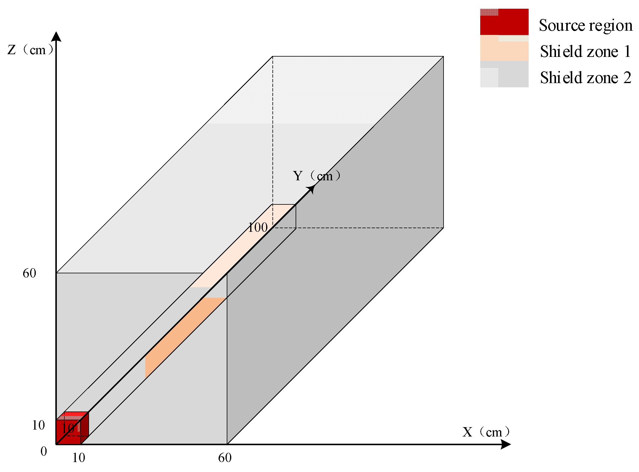
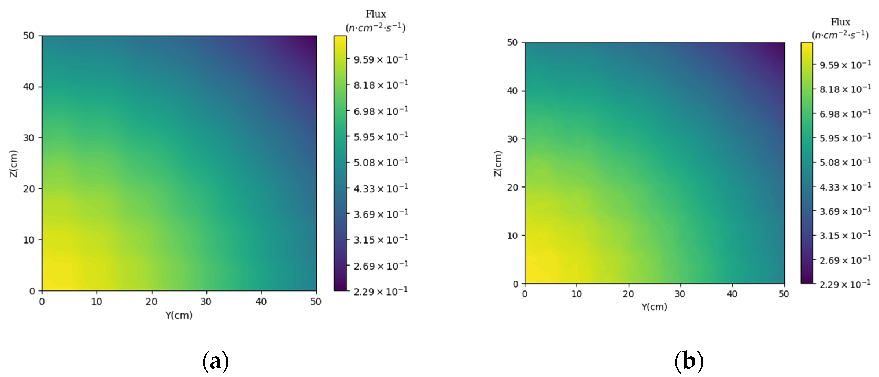
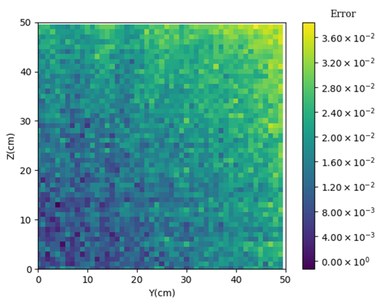
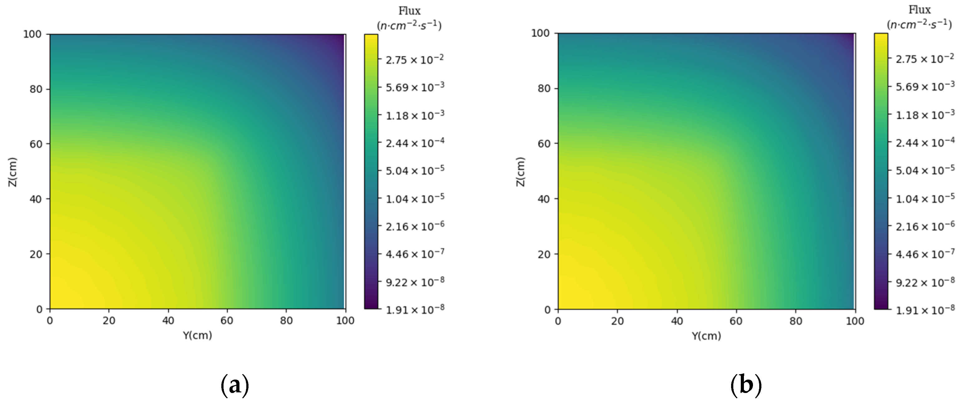
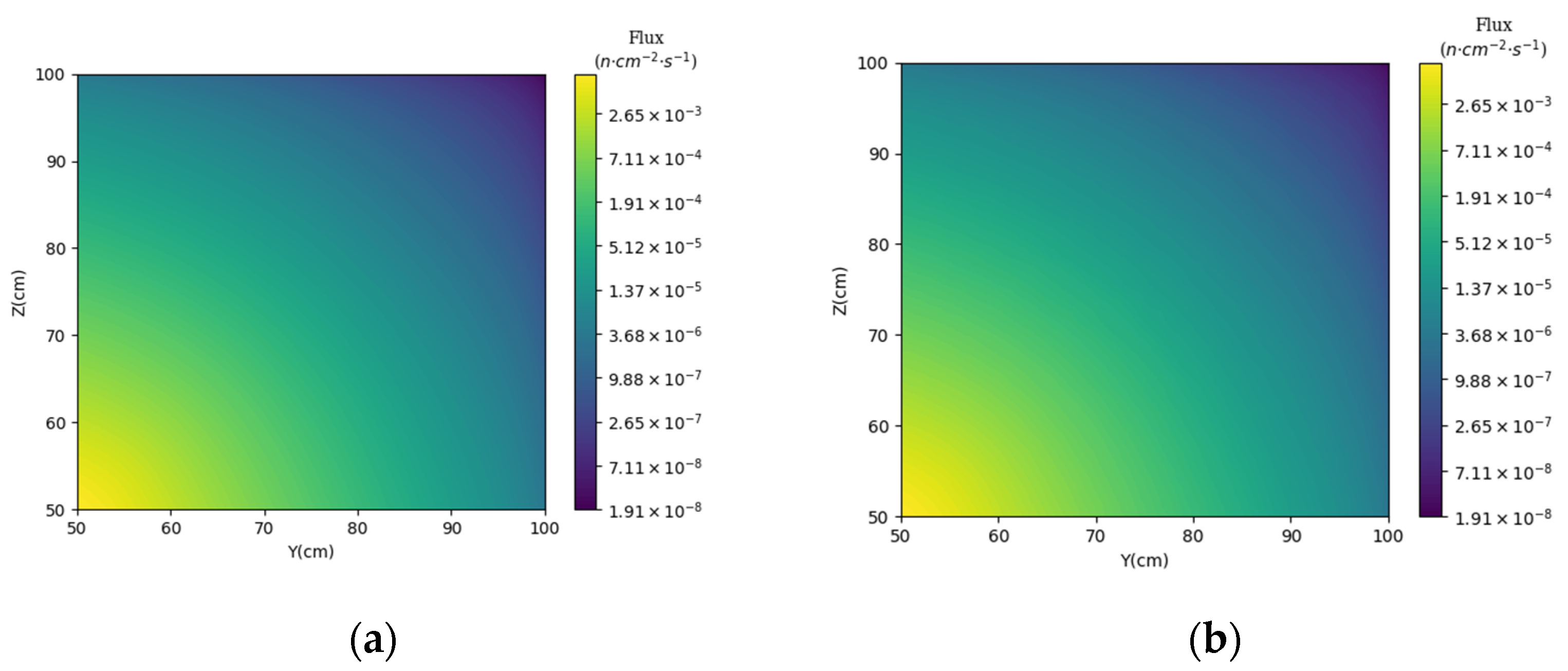
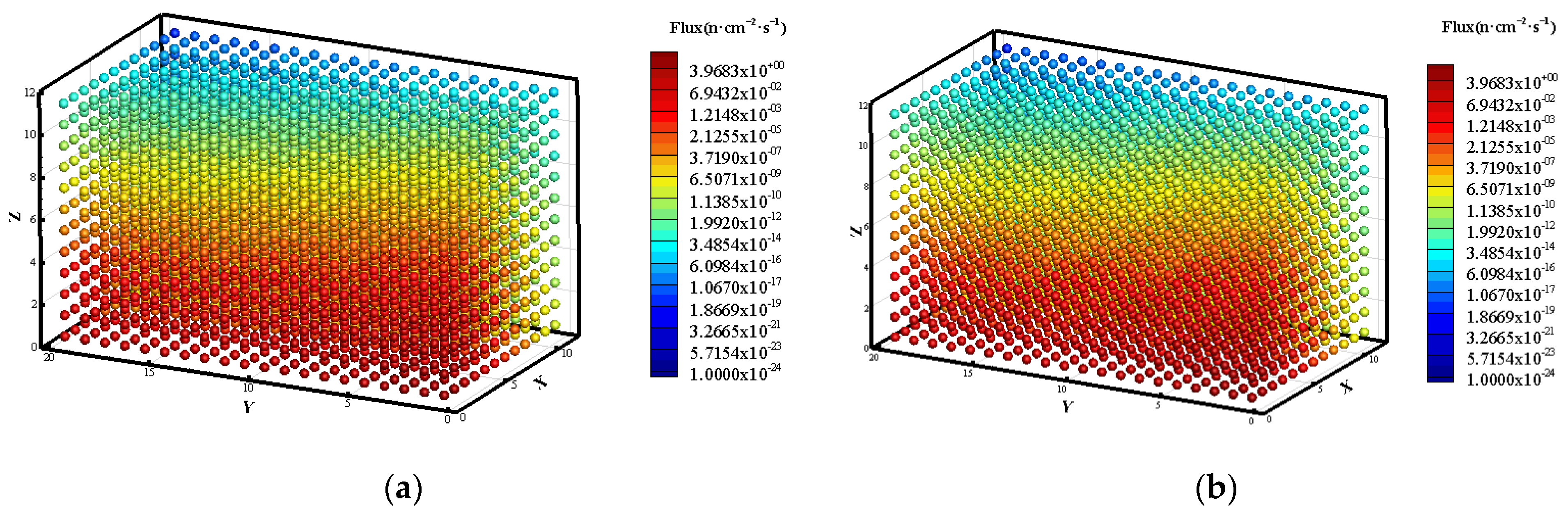
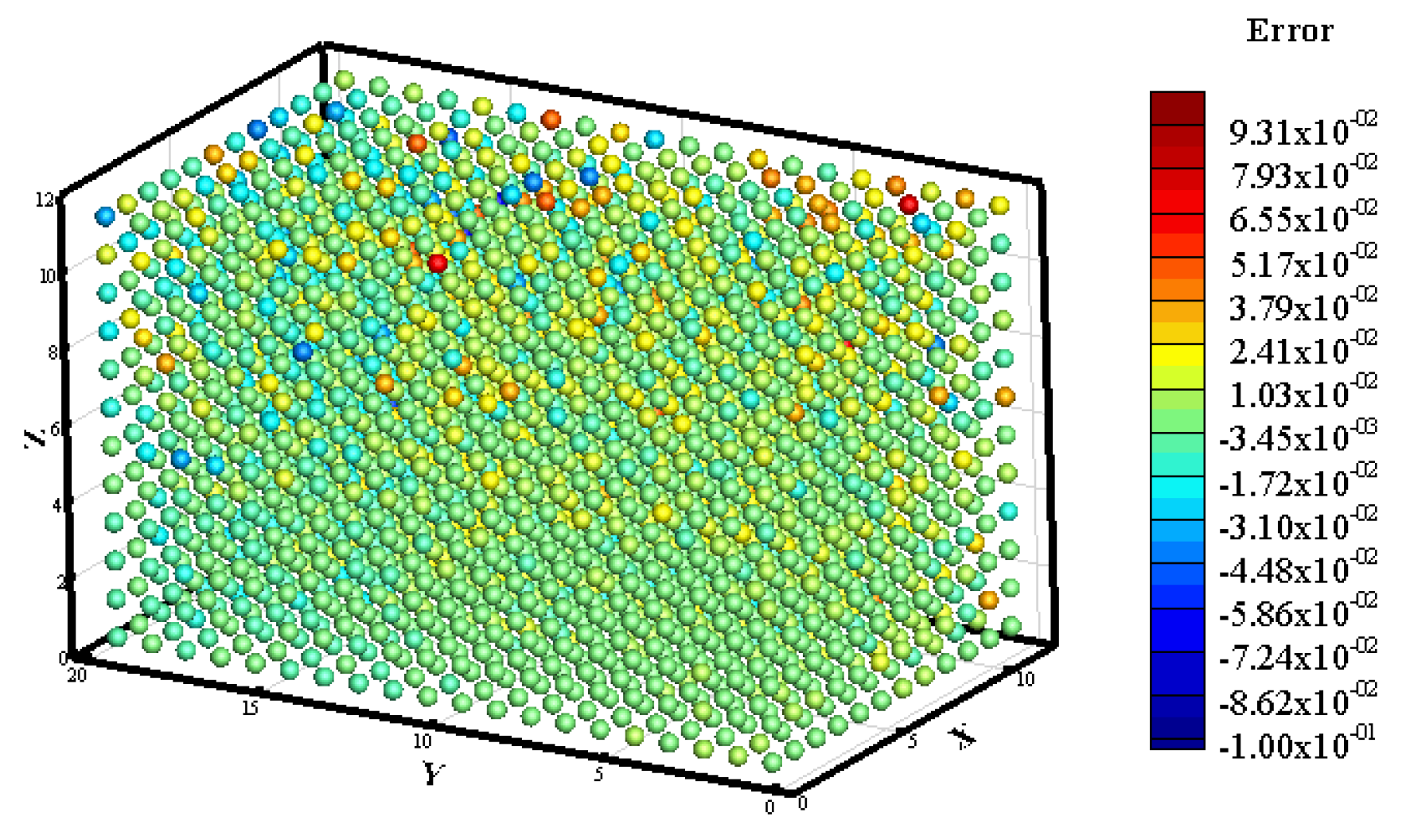
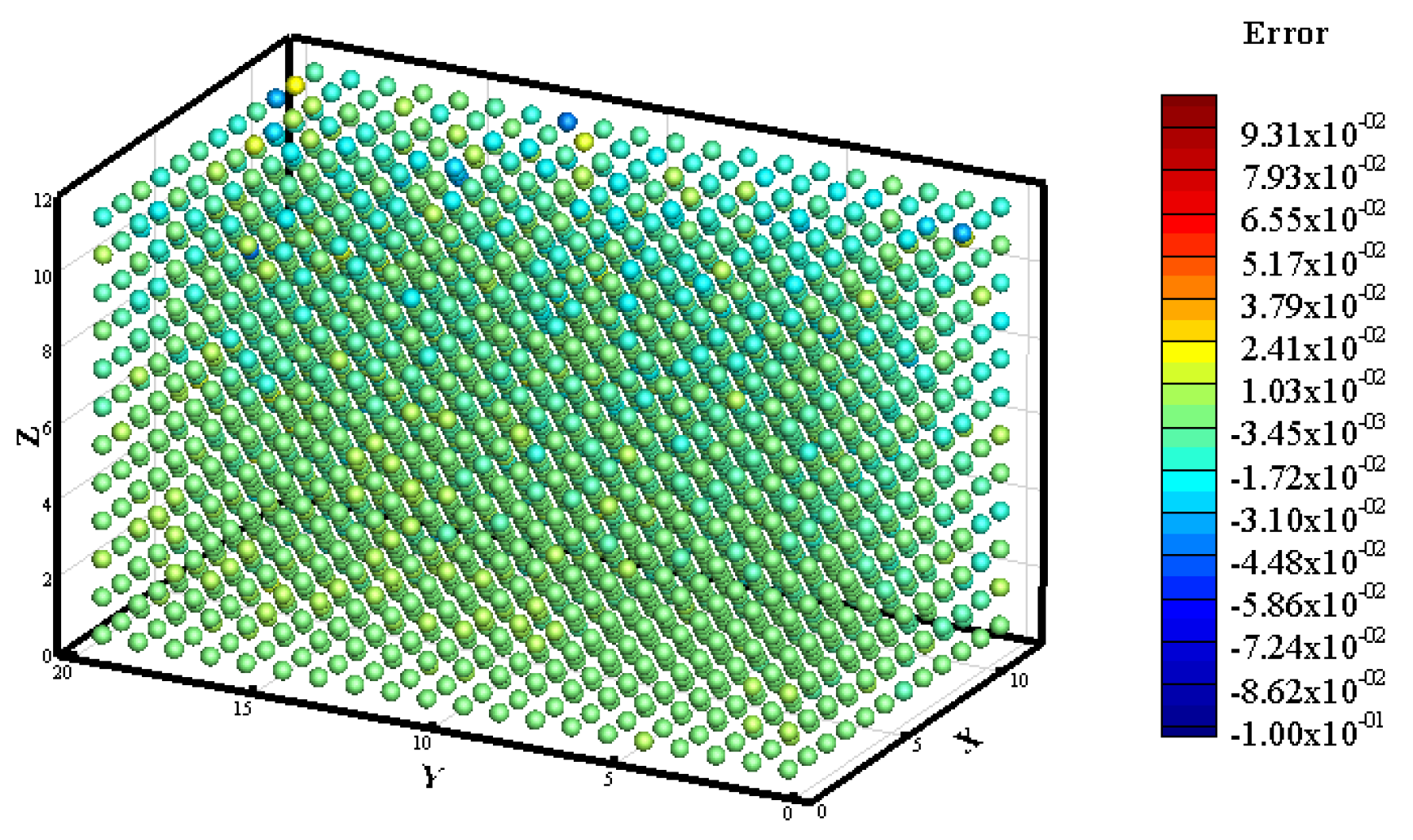
3.1. Prediction of Neutron Flux Distribution in Kobayashi-1 Geometric Shield Region 1

The input layer of Surrogate Model-1 consists of seven neurons, representing the key parameters source strength, total cross-sections and scattering cross-sections of the source region, total cross-sections and scattering cross-sections of Shielding Region 1, and total cross-sections and scattering cross-sections of Shielding Region 2. The output layer contains the neutron flux distribution of 2500 grids at specific coordinates (x = 45.5 cm, 0 cm < y < 50 cm, 0 cm < z < 50 cm), 2500 neurons in total.

The prediction performance of Surrogate Model-1 is verified using three validation use cases and the single prediction time of Surrogate Model-1 is less than 0.1 s. The settings in the transport process using the discrete ordinates method are as follows: the shielding model is divided according to a uniform grid of 1 cm × 1 cm × 1 cm, the EDW scheme is selected, the iterative convergence criterion is 1 × 10⁻³, and the calculation is performed using the quadrature size of order P_NT_N-S₂₄. By comparing the neutron flux distribution (see Figure 6, Figure 7 and Figure 8) and the error Figures (Figure 9, Figure 10 and Figure 11), it is found that the prediction results of the surrogate model are almost consistent with the S_N calculation results under the three validation examples, and the maximum error is 6.00 × 10⁻². In summary, when the flux changes little, the surrogate model can be calculated in 0.1 s while ensuring the accuracy of the discrete ordinates method.

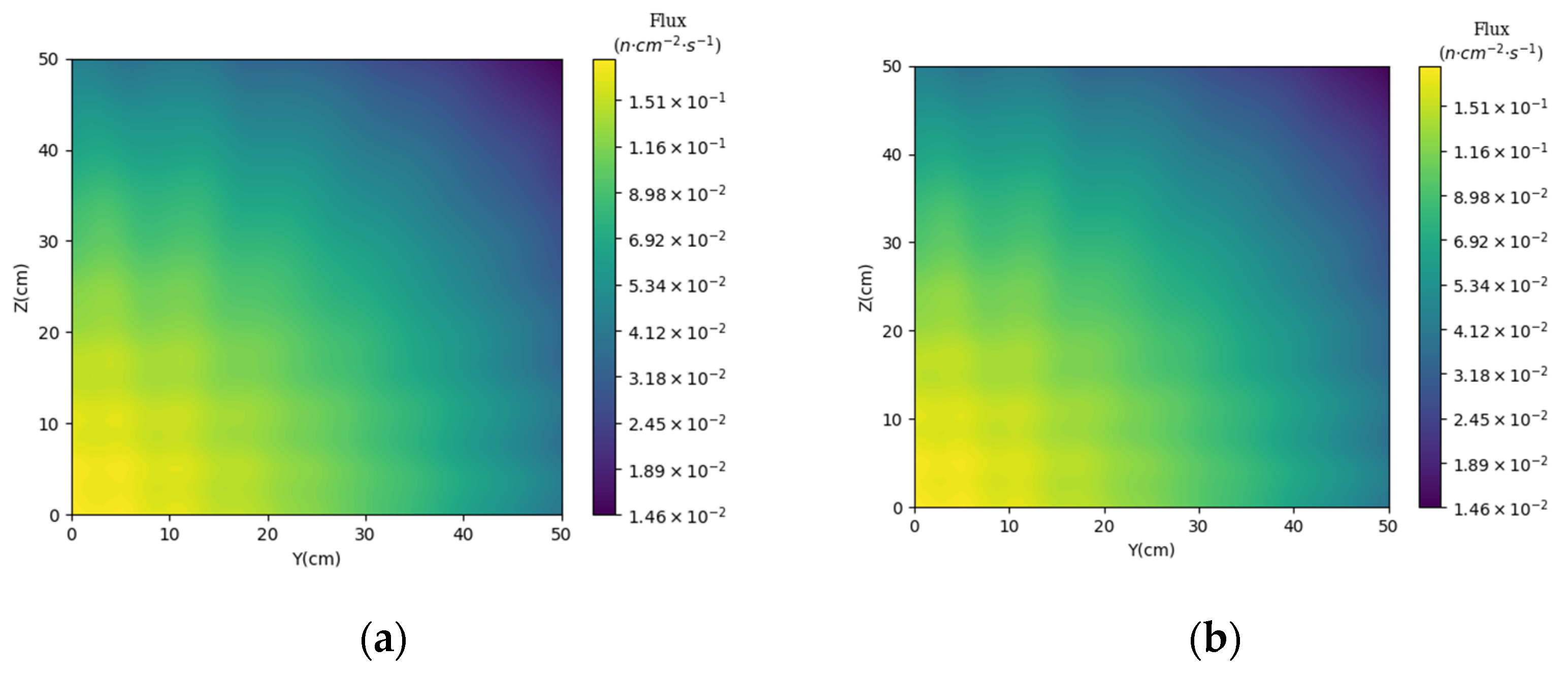
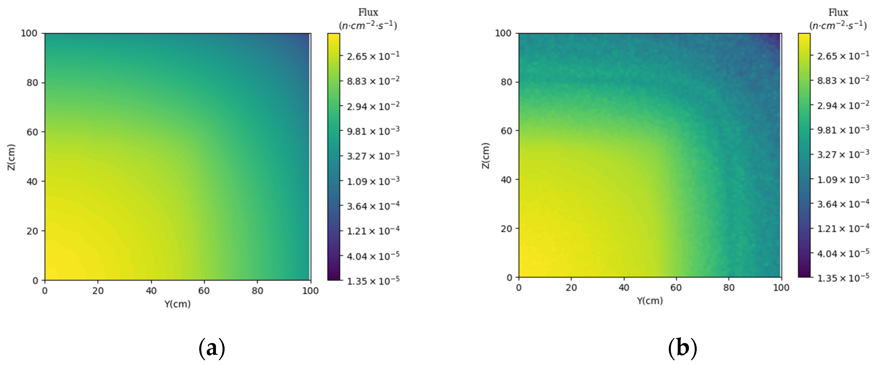
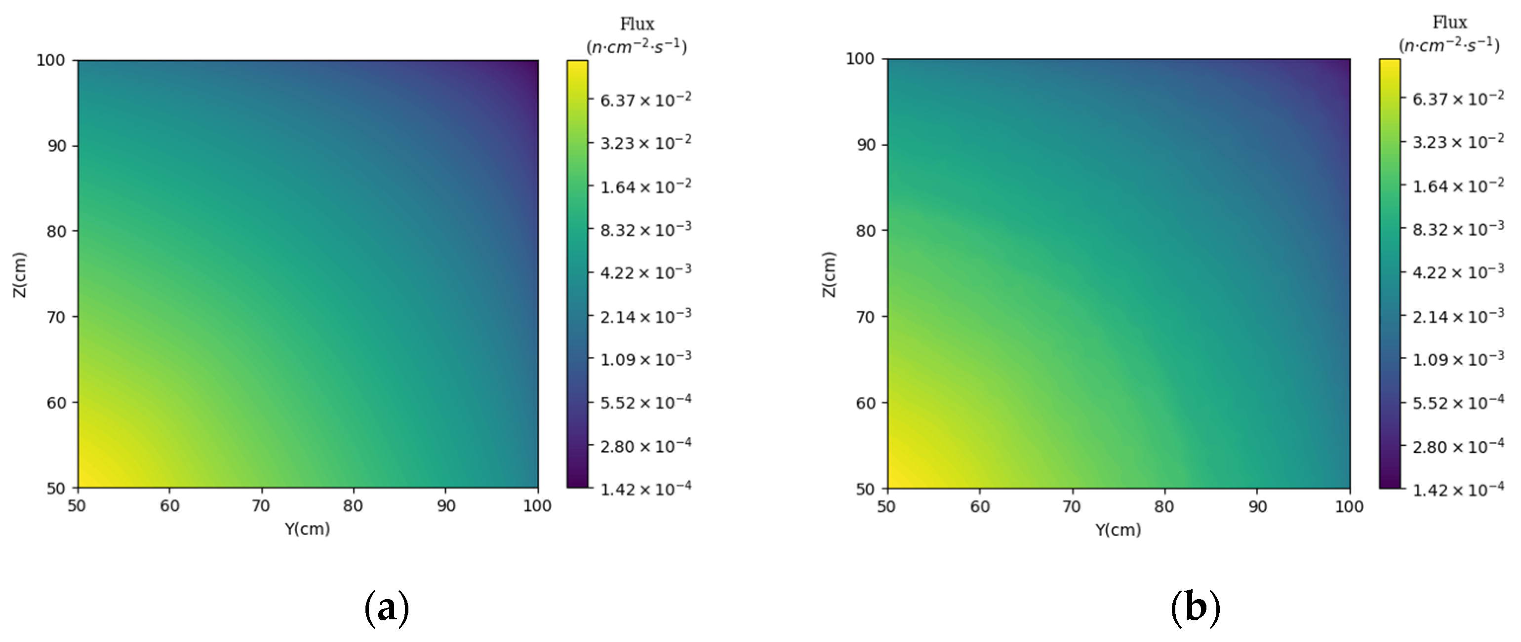
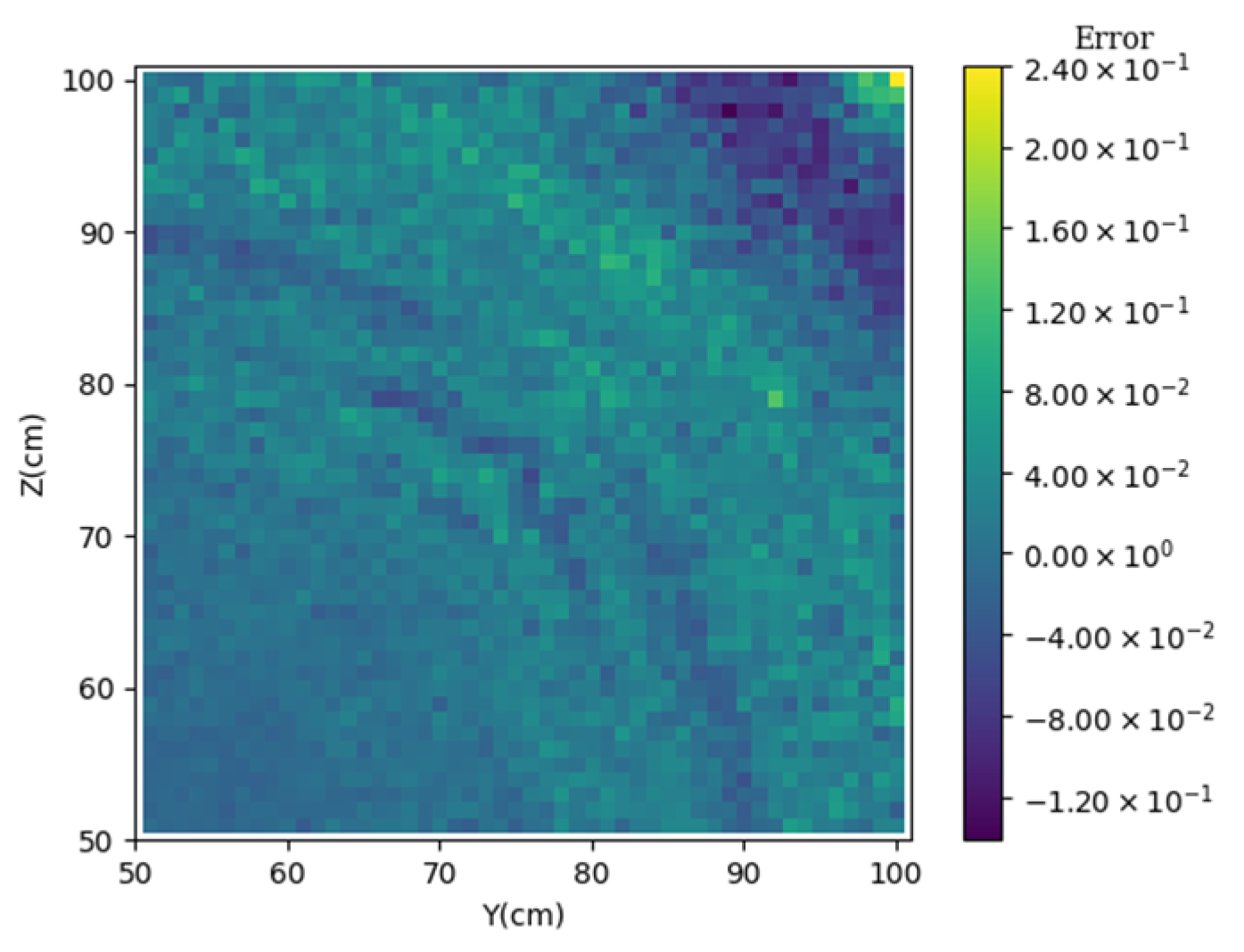
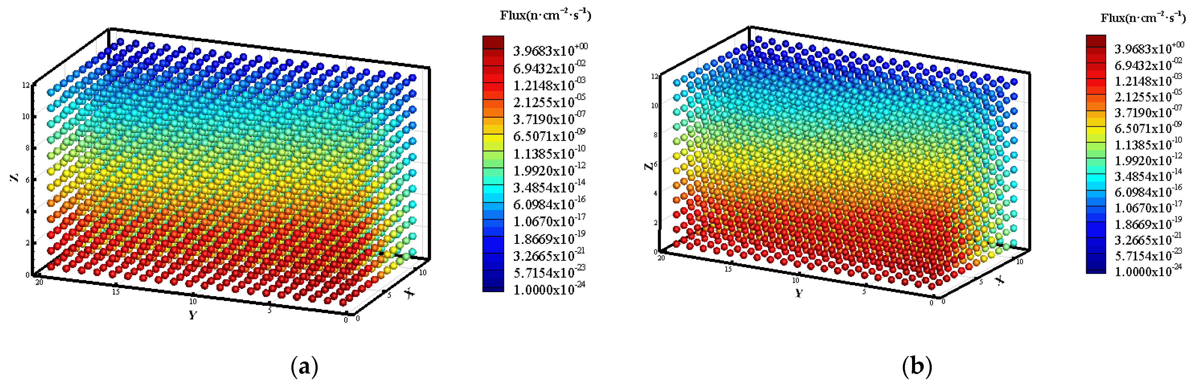
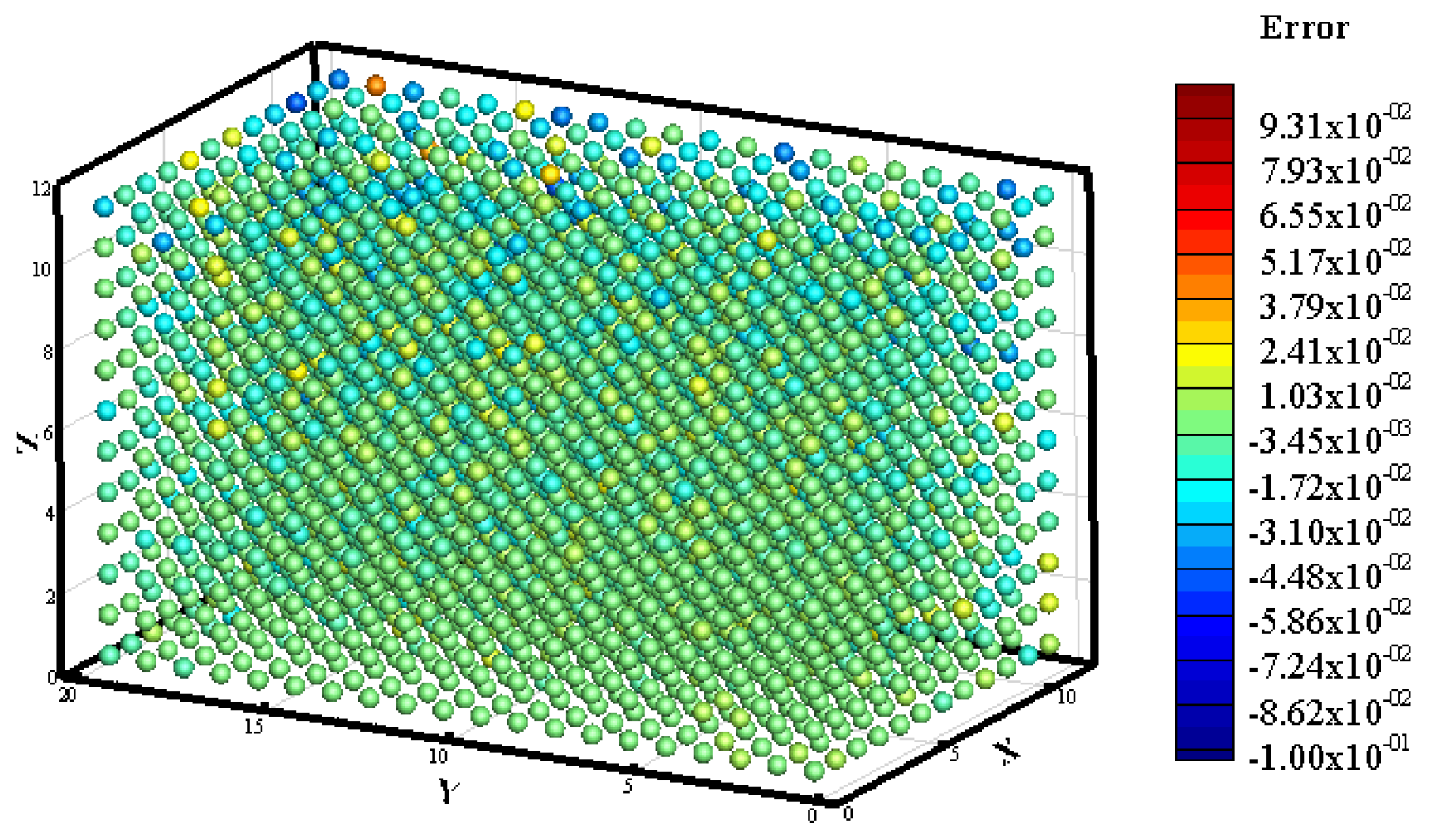
3.2. Prediction of Neutron Flux Distribution in Kobayashi-1 Geometric Shield Region 2

The input layer of the deep learning neural network for Surrogate Model-2 consists of seven neurons, which represent the key parameters source strength, total cross-sections and scattering cross-sections of the source region, total cross-sections and scattering cross-sections of Shielding Region 1, and total cross-sections and scattering cross-sections of Shielding Region 2. The output layer consists of the neutron flux distribution of 10,000 grids at x = 55.5 cm, 0 cm < y < 100 cm, and 0 cm < z < 100 cm.

Three validation use cases are used to verify the prediction performance of Surrogate Model-2. The single prediction time of Surrogate Model-2 was less than 0.1 s. The settings in the transport process using the discrete ordinates method are as follows: the shielding model is divided according to a uniform grid of 1 cm × 1 cm × 1 cm, the EDW scheme is selected, the iterative convergence criterion is 1 × 10⁻³, and the calculation is performed using the quadrature size of order P_NT_N-S₂₄. After comparing the prediction results (see Figure 12, Figure 13, Figure 14, Figure 15, Figure 16 and Figure 17), it is evident that the prediction error of the surrogate model is within ±50% across most of the grids, but the prediction error of the grid with low relative flux is larger in each example, and the prediction error exceeding than ±100%. The performance of the surrogate model becomes increasingly unstable as the flux magnitude and output dimension of the model increase. By comparing Table 10 and Table 12, it can also be found that the test loss of Surrogate Model-2 is significantly higher than that of Surrogate Model-1, which means that Surrogate Model-2 is more difficult to train than Surrogate Model-1. To investigate the cause of this increased prediction error, adjustments were made to align the output dimension of the surrogate model with Surrogate Model-1.

The input layer of Surrogate Model-3 is still composed of seven neurons, which are the source strength of the source region, the total cross-sections and scattering cross-sections of the source region, the total cross-sections and scattering cross-sections of Shield Region 1, and the total cross-sections and scattering cross-sections of Shield Region 2. The output layer consists of the neutron flux distribution of 2500 grids at x = 55.5 cm, 50 cm < y < 100 cm, and 50 cm < z < 100 cm.

Three validation use cases are used to verify the prediction performance of Surrogate Model-3. The single prediction time of Surrogate Model-3 was less than 0.1 s. The settings in the transport process using the discrete ordinates method are as follows: the shielding model is divided according to a uniform grid of 1 cm × 1 cm × 1 cm, the EDW scheme is selected, the iterative convergence criterion is 1 × 10⁻³, and the calculation is performed using the quadrature size of order P_NT_N-S₂₄. By comparing the neutron flux distribution and the error Figures (see Figure 18, Figure 19, Figure 20, Figure 21, Figure 22 and Figure 23), it can be found that the prediction error for most grids is within ±30%, and for grids with large relative flux, the prediction error is within ±45%, while the prediction error of the surrogate model is still large when the neutron flux value is around 1.0 × 10⁻¹⁶. Compared with Surrogate Model-2, Surrogate Model-3 has better prediction ability, and the method of reducing the output dimension effectively improves the prediction accuracy of the model.

The datasets used to build the three surrogate models mentioned above were trained using transport data in the EDW difference scheme. However, the ARES transport code does not take into account angular flux less than 1.0 × 10⁻¹² when using the EDW difference scheme for simulation calculation. As a result, the standard flux near 1.0 × 10⁻¹² is not precise enough for accurate calculation of the value. This is the main reason for the poor performance of the surrogate model on the low flux grid. Therefore, we should pay more attention to the prediction results of the surrogate model on other grids, and the low error of the surrogate model on other grids can also show that the surrogate model constructed by using the deep learning neural network algorithm is feasible and reliable in the neutron flux.

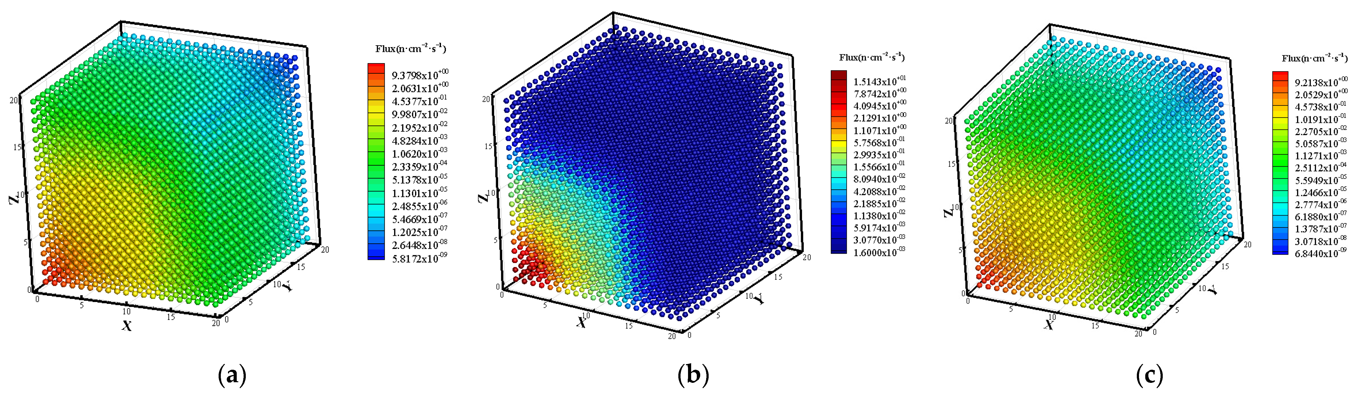
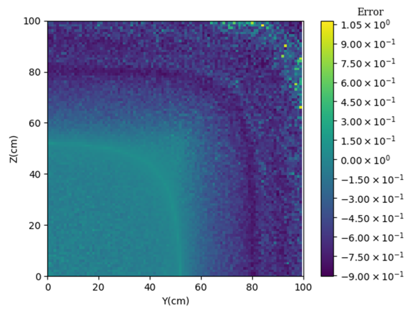
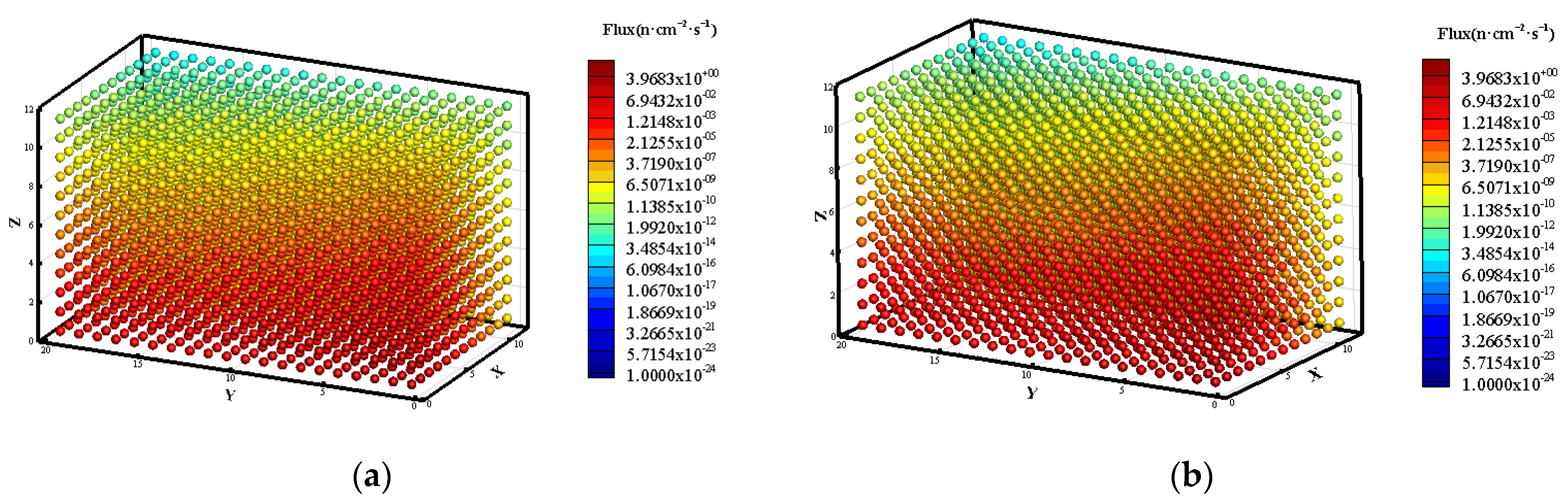
3.3. Prediction of Neutron Flux Distribution in Kobayashi-2 Geometry

The input layer of Surrogate Model-4 is still composed of 16 neurons, which are the source strength of the source region, the total cross-sections and scattering coefficient of the source region, the total cross-sections and scattering coefficient of Shielding Region 1, and the total cross-sections and scattering coefficient of Shielding Region 2. The output layer is the neutron flux of 2880 grids uniformly distributed in the shielded space.

Surrogate Model-4 extends the prediction range from 2D to 3D and is trained on SC transport Dataset-2. Three validation use cases were used to verify the prediction performance of Surrogate Model-4, and the prediction time of Surrogate Model-3 did not exceed 0.1 s. The settings in the transport process using the discrete ordinates method are as follows: the shielding model is divided according to a uniform grid of 1 cm × 1 cm × 1 cm, the SC scheme is selected, the iterative convergence criterion is 1 × 10⁻³, and the calculation is performed using the quadrature size of order P_NT_N-S₂₄. By comparing the calculated results of S_N with those of Surrogate Model-4 (see Figure 24, Figure 25, Figure 26, Figure 27, Figure 28 and Figure 29), it can be seen that the error of the prediction results of the surrogate model on all grids does not exceed 10% in the face of three validation use cases with different characteristics. This clearly indicates that the high prediction error of Surrogate Model-2 and Surrogate Model-3 in the previous section, on the grid with actual flux less than 1.0 × 10⁻¹², is not due to inadequate training of the surrogate model. In summary, the surrogate model can be calculated in 0.1 s while ensuring the accuracy of the discrete ordinates method.

The comparison of the training processes and calculation results of the four surrogate models reveals that Surrogate Model-1, Surrogate Model-3, and Surrogate Model-4 exhibit reduced train and test losses, as well as lower calculation errors. This indicates that when the output dimension of the surrogate model is below 2500, it is associated with higher calculation accuracy and a more straightforward training process. In a similar context, the prediction outcome of Surrogate Model-1 exhibited superior accuracy in comparison to the other surrogate models, suggesting that the surrogate model is capable of effective prediction in the presence of minor flux variations. In the context of significant flux variation, a larger output dimension (Surrogate Model-3) is likely to result in a reduction in the calculation accuracy of the surrogate model. Surrogate Model-4 extends the prediction position to three-dimensional space. The calculation results demonstrate that the calculation accuracy of Surrogate Model-4 is less than 10% for the strong anisotropy problem.

4. Summary

This paper explores a rapid method for obtaining neutron flux distribution using deep learning techniques. Geometric models based on Kobayashi-1 and Kobayshi-2 utilize the discrete ordinates method to generate comprehensive training data. A deep learning neural network is employed to train four surrogate models capable of predicting the neutron flux distribution at various locations. By constructing the dataset with information related to the discrete ordinates method, the interpretability between the input (transport parameters) and output (neutron flux) is enhanced, leading to improved reliability of the surrogate model. Experimental results demonstrate that each individual prediction time of the surrogate model is less than 0.1 s. In terms of prediction accuracy, transport parameters with varying characteristics were utilized to validate the predictive performance of each surrogate model, the reasons for the high grid errors in the prediction results were elucidated. The predicted grid position was expanded from two dimensions to three dimensions. The efficacy of the surrogate model in neutron flux calculations is demonstrated through a comparison of the prediction accuracy between the surrogate models trained with EDW and SC transport datasets. The surrogate model is capable of effectively maintaining prediction accuracy below 10%. Future research should consider more practical engineering problems, compare the results with those of other numerical calculation methods, and summarize and analyze the advantages and disadvantages of surrogate models and other numerical calculation methods.

References

1. Bell, G.I.; Glasstone, S. Nuclear Reactor Theory; US Atomic Energy Commission: Washington, DC, USA, 1970. [Google Scholar]
2. Larsen, E.W. An Overview of Neutron Transport Problems and Simulation Techniques. Comput. Methods Transp. 2004, 48, 513–533. [Google Scholar] [CrossRef]
3. Lewis, E.E.; Miller, W.F. Computational Methods of Neutron Transport; John Wiley and Sons, Inc.: New York, NY, USA, 1993. [Google Scholar]
4. Adams, M.L.; Larsen, E.W. Fast Iterative Methods for Discrete Ordinates Particle Transport Calculations. Prog. Nucl. Energy 2012, 40, 3–159. [Google Scholar] [CrossRef]
5. Gong, C.Y.; Liu, J.; Chi, L.H.; Huang, H.W.; Fang, J.Y.; Gong, Z.H. GPU Accelerated Simulations of 3D Deterministic Particle Transport Using Discrete Ordinates Method. J. Comput. Phys. 2011, 230, 6010–6022. [Google Scholar] [CrossRef]
6. Baker, R.S.; Koch, K.R. An SN Algorithm for the Massively Parallel CM-200 Computer. Nucl. Sci. Eng. 1998, 128, 312–320. [Google Scholar] [CrossRef]
7. Plimpton, S.; Hendrickson, B.; Burns, S.; McLendon, W. Parallel Algorithms for Radiation Transport on Unstructured Grids. In Proceedings of the SC ’00: Proceedings of the 2000 ACM/IEEE Conference on Supercomputing, Dallas, TX, USA, 4–10 November 2000; p. 25. [Google Scholar] [CrossRef]
8. Mo, Z.Y.; Zhang, A.Y.; Zhang, Y. A New Parallel Algorithm for Vertex Priorities of Data Flow Acyclic Digraphs. J. Supercomput. 2014, 68, 49–64. [Google Scholar] [CrossRef]
9. Baker, R.S. A Block Adaptive Mesh Refinement Algorithm for the Neutral Particle Transport Equation. Nucl. Sci. Eng. 2002, 141, 1–12. [Google Scholar] [CrossRef]
10. Zhang, H.; Lewis, E.E. Spatial Adaptivity Applied to the Variational Nodal PN Equations. Nucl. Sci. Eng. 2002, 142, 57–63. [Google Scholar] [CrossRef]
11. Wang, Y.Q.; Ragusa, J.C. Application of hp Adaptivity to the Multigroup Diffusion Equations. Nucl. Sci. Eng. 2009, 161, 22–48. [Google Scholar] [CrossRef]
12. Lathouwers, D. Goal-Oriented Spatial Adaptivity for the SN Equations on Unstructured Triangular Meshes. Ann. Nucl. Energy 2011, 38, 1373–1381. [Google Scholar] [CrossRef]
13. Zhang, B.; Zhang, L.; Liu, C.; Chen, Y.X. Goal-Oriented Regional Angular Adaptive Algorithm for the SN Equations. Nucl. Sci. Eng. 2018, 189, 120–134. [Google Scholar] [CrossRef]
14. Zhang, L.; Zhang, B.; Chen, Y.X. Spatial Adaptive Algorithm for Discrete Ordinates Shielding Calculation. At. Energy Sci. Technol. 2018, 52, 2233–2242. (In Chinese) [Google Scholar] [CrossRef]
15. Liu, C.; Zhang, B.; Zhang, L.; Chen, Y.X. Nonmatching Discontinuous Cartesian Grid Algorithm Based on the Multilevel Octree Architecture for Discrete Ordinates Transport Calculation. Nucl. Sci. Eng. 2020, 194, 1175–1201. [Google Scholar] [CrossRef]
16. Liu, C.; Zhang, B.; Wang, X.Y.; Zhang, L.; Chen, Y.X. Reformulation and Evaluation of Robust Characteristic-based Discretization for the Discrete Ordinates Equation on Structured Hexahedron Grids. Prog. Nucl. Energy 2020, 126, 103403. [Google Scholar] [CrossRef]
17. Allen, E.J. Stochastic Difference Equations and A Stochastic Partial Differential Equation for Neutron Transport. J. Differ. Equ. Appl. 2012, 18, 1267–1285. [Google Scholar] [CrossRef]
18. Hajas, T.Z.; Tolnai, G.; Margoczi, M.; Legrady, D. Noise Term Modeling of Dynamic Monte Carlo Using Stochastic Differential Equations. Ann. Nucl. Energy 2024, 195, 110061. [Google Scholar] [CrossRef]
19. Berry, J.J.; Gil-Delgado, G.G.; Osborne, A.G.S. Classification of Group Structures for a Multigroup Collision Probability Model Using Machine Learning. Ann. Nucl. Energy 2021, 160, 108367. [Google Scholar] [CrossRef]
20. Schmidhuber, J. Deep Learning in Neural Networks: An Overview. Neural Netw. 2015, 61, 85–117. [Google Scholar] [CrossRef] [PubMed]
21. Zhou, W.; Sun, G.M.; Yang, Z.H.; Wang, H.; Fang, L.; Wang, J.Y. BP Neural Network Based Reconstruction Method for Radiation Field Applications. Nucl. Eng. Des. 2021, 380, 111228. [Google Scholar] [CrossRef]
22. Li, Z.G.; Sun, J.; Wei, C.L.; Sui, Z.; Qian, X.Y. A New Cross-sections Calculation Method in HTGR Engineering Simulator System Based on Machine Learning Methods. Ann. Nucl. Energy 2020, 145, 107553. [Google Scholar] [CrossRef]
23. Zhu, Q.J.; Tian, L.C.; Yang, X.H.; Gan, L.F.; Zhao, N.; Ma, Y.Y. Advantages of artificial neural network in neutron spectra unfolding. Chin. Phys. Lett. 2014, 31, 69–72. [Google Scholar] [CrossRef]
24. Cao, C.L.; Gan, Q.; Song, J.; Long, P.C.; Wu, B.; Wu, Y.C. A Two-Step Neutron Spectrum Unfolding Method for Fission Reactors Based on Artificial Neural Network. Ann. Nucl. Energy 2019, 139, 107219. [Google Scholar] [CrossRef]
25. dos Santos, M.C.; Pinheiro VH, C.; do Desterro FS, M.; de Avellar, R.K.; Schirru, R.; dos Santos Nicolau, A.; de Lima, A.M.M. Deep Rectifier Neural Network Applied to the Accident Identification Problem in A PWR Nuclear Power Plant. Ann. Nucl. Energy 2019, 133, 400–408. [Google Scholar] [CrossRef]
26. Cao, C.L.; Gan, Q.; Song, J.; Long, P.C.; Wu, B.; Wu, Y.C. An Artificial Neural Network-based Neutron Field Reconstruction Method for Reactor. Ann. Nucl. Energy 2020, 138, 107195. [Google Scholar] [CrossRef]
27. Song, Y.M.; Zhao, Y.B.; Li, X.X.; Wang, K.; Zhang, Z.H.; Luo, W.; Zhu, Z.C. A Method for Optimizing the Shielding Structure of Marine Reactors. Nucl. Sci. Eng. 2017, 37, 355–361. (In Chinese) [Google Scholar]
28. Song, Y.M.; Zhang, Z.H.; Mao, J.; Lu, C.; Tang, S.Q.; Xiao, F.; Lyu, H.W. Research on Fast Intelligence Multi-objective Optimization Method of Nuclear Reactor Radiation Shielding. Ann. Nucl. Energy 2020, 149, 107771. [Google Scholar] [CrossRef]
29. Vasseur, A.; Makovicka, L.; Martin, É.; Sauget, M.; Contassot-Vivier, S.; Bahi, J. Dose Calculations Using Artificial Neural Networks: A Feasibility Study for Photon Beams. Nucl. Instrum. Methods Phys. Res. Sect. B Beam Interact. Mater. At. 2018, 266, 1085–1093. [Google Scholar] [CrossRef]
30. Wang, J.; Peng, X.; Chen, Z. Surrogate Modeling for Neutron Diffusion Problems Based on Conservative Physics-informed Neural Networks with Boundary Conditions Enforcement. Ann. Nucl. Energy 2022, 176, 109234. [Google Scholar] [CrossRef]
31. Yann, L.C.; Bengio, Y.; Hinton, G. Deep Learning. Nature 2015, 521, 436–444. [Google Scholar] [CrossRef]
32. Fowler, T.B.; Vondy, D.R. Nuclear Reactor Core Analysis Code; ORNL-TM-2496; Oak Ridge National Laboratory (ORNL): Oak Ridge, TN, USA, 1969. [Google Scholar]
33. Semenza, L.A.; Lewis, E.E.; Rossow, E.C. The Application of the Finite Element Method to the Multigroup Neutron Diffusion Equation. Nucl. Sci. Eng. 1972, 47, 302–310. [Google Scholar] [CrossRef]
34. Chen, Y.X.; Zhang, B.; Zhang, L.; Zheng, J.X.; Zheng, Y.; Liu, C. ARES: A Parallel Discrete Ordinates Transport Code for Radiation Shielding Applications and Reactor Physics Analysis. Sci. Technol. Nucl. Ins. 2017, 2017, 2596727. [Google Scholar] [CrossRef]
35. Kobayashi, K.; Sugimura, N.; Nagaya, Y. 3D Radiation Transport Benchmark Problems and Results for Simple Geometries with Void Region. Prog. Nucl. Energy 2001, 39, 119–144. [Google Scholar] [CrossRef]
36. Abadi, M.; Agarwal, A.; Barham, P.; Brevdo, E.; Chen, Z.; Citro, C.; Zheng, X. TensorFlow: Large Scale Machine Learning on Heterogeneous Distributed Systems. In Proceedings of the 12th USENIX Symposium on Operating Systems Design and Implementation (OSDI 16), Savannah, GA, USA, 2–4 November 2016; pp. 265–283. [Google Scholar]
37. Glorot, X.; Bengio, Y. Understanding the Difficulty of Training Deep Feedforward Neural Networks. In Proceedings of the Thirteenth International Conference on Artificial Intelligence and Statistics, Sardinia, Italy, 13–15 May 2010; pp. 249–256. [Google Scholar]
38. Clevert, D.A.; Unterthiner, T.; Hochreiter, S. Fast and Accurate Deep Network Learning by Exponential Linear Units (elus). arXiv 2015, arXiv:1511.07289. [Google Scholar]
39. Kingma, D.P.; Ba, J. Adam: A Method for Stochastic Optimization. arXiv 2014, arXiv:1412.6980. [Google Scholar]
40. Smith, L.N. A Disciplined Approach to Neural Network Hyperparameters: Part 1–Learning Rate, Batch Size, Momentum, and Weight Decay. arXiv 2018, arXiv:1803.09820. [Google Scholar]
Figure 1. Basic structure of the neural network.
Energies 17 03440 g001
Figure 2. Kobayashi-1 geometry model.
Energies 17 03440 g002
Figure 3. Kobayashi-2 geometry model.
Energies 17 03440 g003
Figure 4. The fitting results of the neural network. (a) SN calculation, (b) no standardization, (c) log standardization.
Energies 17 03440 g004
Figure 5. Prediction of neutron flux distributions by deep learning neural network.
Energies 17 03440 g005
Figure 6. Comparison of neutron flux for validation use case 1: (a) SN calculation, (b) Surrogate Model-1 prediction.
Energies 17 03440 g006
Figure 7. Comparison of neutron flux for validation use case 2: (a) SN calculation, (b) Surrogate Model-1 prediction.
Energies 17 03440 g007
Figure 8. Comparison of neutron flux for validation use case 3: (a) SN calculation, (b) Surrogate Model-1 prediction.
Energies 17 03440 g008
Figure 9. Validation use case 1: The error between SN calculation and Surrogate Model-1 prediction.
Energies 17 03440 g009
Figure 10. Validation use case 2: The error between SN calculation and Surrogate Model-1 prediction.
Energies 17 03440 g010
Figure 11. Validation use case 3: The error between SN calculation and Surrogate Model-1 prediction.
Energies 17 03440 g011
Figure 12. Comparison of neutron flux for validation use case 1: (a) SN calculation, (b) Surrogate Model-2 prediction.
Energies 17 03440 g012
Figure 13. Comparison of neutron flux for validation use case 2: (a) SN calculation, (b) Surrogate Model-2 prediction.
Energies 17 03440 g013
Figure 14. Comparison of neutron flux for validation use case 3: (a) SN calculation, (b) Surrogate Model-2 prediction.
Energies 17 03440 g014
Figure 15. Validation use case 1: The error between SN calculation and Surrogate Model-2 prediction.
Energies 17 03440 g015
Figure 16. Validation use case 2: The error between SN calculation and Surrogate Model-2 prediction.
Energies 17 03440 g016
Figure 17. Validation use case 3: The error between SN calculation and Surrogate Model-2 prediction.
Energies 17 03440 g017
Figure 18. Comparison of neutron flux for validation use case 1: (a) SN calculation, (b) Surrogate Model-3 prediction.
Energies 17 03440 g018
Figure 19. Comparison of neutron flux for validation use case 2: (a) SN calculation, (b) Surrogate Model-3 prediction.
Energies 17 03440 g019
Figure 20. Comparison of neutron flux for validation use case 3: (a) SN calculation, (b) Surrogate Model-3 prediction.
Energies 17 03440 g020
Figure 21. Validation use case 1: The error between SN calculation and Surrogate Model-3 prediction on 2500 grids at x = 55.5 cm, 50 cm < y < 100 cm, and 50 cm < z < 100 cm.
Energies 17 03440 g021
Figure 22. Validation use case 2: The error between SN calculation and Surrogate Model-3 prediction on 2500 grids at x = 55.5 cm, 50 cm < y < 100 cm, and 50 cm < z < 100 cm.
Energies 17 03440 g022
Figure 23. Validation use case 3: The error between SN calculation and Surrogate Model-3 prediction on 2500 grids at x = 55.5 cm, 50 cm < y < 100 cm, and 50 cm < z < 100 cm.
Energies 17 03440 g023
Figure 24. Comparison of neutron flux for validation use case 4: (a) SN calculation, (b) Surrogate Model-4 prediction.
Energies 17 03440 g024
Figure 25. Comparison of neutron flux for validation use case 5: (a) SN calculation, (b) Surrogate Model-4 prediction.
Energies 17 03440 g025
Figure 26. Comparison of neutron flux for validation use case 6: (a) SN calculation, (b) Surrogate Model-4 prediction.
Energies 17 03440 g026
Figure 27. Validation use case 4: The error between SN calculation and Surrogate Model-4 prediction.
Energies 17 03440 g027
Figure 28. Validation use case 5: The error between SN calculation and Surrogate Model-4 prediction.
Energies 17 03440 g028
Figure 29. Validation use case 6: The error between SN calculation and Surrogate Model-4 prediction.
Energies 17 03440 g029