Abstract
In this paper, the new non-integer-order state space model of heat processes in a one-dimensional metallic rod is addressed. The fractional orders of derivatives along space and time are not exactly known, and they are described by intervals. The proposed model is the interval expanding of the state space fractional model of heat conduction and dissipation in a one-dimensional metallic rod. It is expected to better describe reality because the interval order of each real process is difficult to estimate. Using intervals enables describing the uncertainty. The presented interval model can be applied to the modeling of many real thermal processes in the industry and building. For example, it can describe the thermal conductivity of building walls. The one-dimensional approach can be applied because only the direction from inside to outside is important, and the heat distribution along the remaining directions is uniform. The paper describes the basic properties of the proposed model and supports the theory via simulations in MATLAB R2020b and experiments executed with the use of a real experimental laboratory system equipped with miniature temperature sensors and supervised by PLC and SCADA systems. The main results from the paper point out that the uncertainty of both fractional orders impacts the crucial properties of the model. The uncertainty of the derivative along the time affects only the dynamics, but the disturbance of the derivative along the length disturbs both the static and dynamic properties of the model.
1. Introduction
The results of many authors have been indicating for years that the FO calculus serves as a very convenient tool to describe many physical, biological, and social processes.
Fundamental examples of such models were provided, e.g., in [1,2] (thermal processes in a one-dimensional beam), ref. [3] (FO models of chaotic systems and Ionic Polymer Metal Composites), and [4]. Non-integer-order models of diffusion processes were presented, for example, in [5,6,7]. The results of presenting the use of a new Atangana–Baleanu operator were provided in [8]. They covered among others the FO blood alcohol model, the Christov diffusion equation, and the fractional advection–dispersion equation for groundwater transport processes.
Recently, FO models have been applied to describe the spread of diseases, such as FO models of the dynamics of COVID-19 using the Caputo–Fabrizio operator presented by [9] or the model of the transmission of the Zika virus using the Atangana–Baleanu operator proposed by [10].
Models of temperature fields have been considered by many authors, e.g., [11,12]. New, dimensionless cost functions describing the exergy of a heat exchanger were proposed in [13]. The two-dimensional IO heat transfer equation was analytically solved in [14]. The numerical methods of the solution of PDEs were provided by various authors, e.g., in [15]. Fractional Fourier integral operators were analyzed in [16]. Most of the known results described only steady-state temperature fields while omitting their dynamics.
The recent results from the area of the modeling of the thermal processes in the industry cover, among others, the modeling of the thermal processes in gas distribution systems [17].
FO models of one-dimensional heat transfer in the state space have been proposed in many previous papers of authors from the years 2016–2018 and 2020 [18,19,20,21,22,23,24,25]. In the proposed models, different FO operators were employed. There were Grünwald–Letnikov, Caputo, Caputo–Fabrizio, and Atangana–Baleanu, as well as discrete operators CFE and FOBD. Each proposed model has been thoroughly justified theoretically and experimentally. The accuracy of each FO model regarding the square cost function was better than its IO analogue.
The sensitivity of the FO model to the uncertainty of the coefficients describing the heat conduction and heat exchange was considered in [26]. In this paper, the uncertainty of the fractional orders was not considered. Such an analysis is provided in this paper.
The papers [27,28] presented the two-dimensional generalization of the FO models proposed previously.
This article presents the generalization of the model provided in [22] to the case when both fractional orders are described by intervals. Such an approach should better describe reality because the fractional orders are difficult to estimate in contrast to the parameters describing heat transfer and heat conduction. Based on the knowledge of the author, such a model has not been proposed yet. The interval fractional-order system was considered, e.g., by [29], but this paper deals with the interval state operator and known interval order of the derivative in relation to time.
The organization of the paper is as follows. The preliminaries provide the basic ideas from fractional calculus that are necessary to explain the main results. Next, the experimental system and its FO model with interval orders are proposed and analyzed. Finally, the experimental validation of the theoretical results is shown.
2. Preliminaries
Preliminaries will start with defining of the non-integer-order integro-differential operator (see, e.g., [1,4,30,31]).
Definition 1
(The basic non-integer-order operator). The fractional-order integro-differential operator is defined as follows:
where a and t are time limits for operator computing and is the fractional order of the operation.
In (1), the positive value of denotes the derivation, and its negative value describes the integration. Simultaneously, for integer values of , this definition describes IO derivation or integration. The next significant difference is that a fractional derivative is computed on an interval and not at a point.
Next, recall an idea of complete Gamma Euler function (see, e.g., [31]):
Definition 2
(The complete Gamma function).
Function (2) is the generalization of factorial to real numbers.
Next, recall the two-parameter Mittag-Leffler function. It is a non-integer-order generalization of exponential function and plays a crucial role in the solution of an FO state equation. It is defined as follows:
Definition 3
(The two-parameter Mittag-Leffler function).
For , the two-parameter function reduces to the one-parameter Mittag-Leffler function:
Definition 4
(The one-parameter Mittag-Leffler function).
The FO operator (1) can be expressed by three fundamental definitions, formulated by Grünwald and Letnikov (GL definition), Riemann and Liouville (RL definition), and Caputo (C definition). Relationships between Caputo and Riemann–Liouville and between Riemann–Liouville and Grünwald–Letnikov operators are proven, for example, in [4,32]. Discrete versions of these operators are deeply analyzed by [33]. The C definition has intuitive interpretation of an initial condition as well as Laplace transform. Additionally, its value from a constant equals to zero, in contrast to, e.g., RL definition. That is why the C definition will be applied in this paper. It is provided below.
Definition 5
(The Caputo definition of the FO operator).
In (5), V describes a limiter of the non-integer order . For , the order of operation lies in the range , and the definition of (5) takes the form
Finally, a fractional linear state equation employing the C definition should be recalled. It is as follows:
where denotes the fractional order of the state equation, , , and denote the state, control, and output vectors, respectively, and are the state, control, and output matrices.
3. The Experimental System and Its Model with Fractional Interval Orders
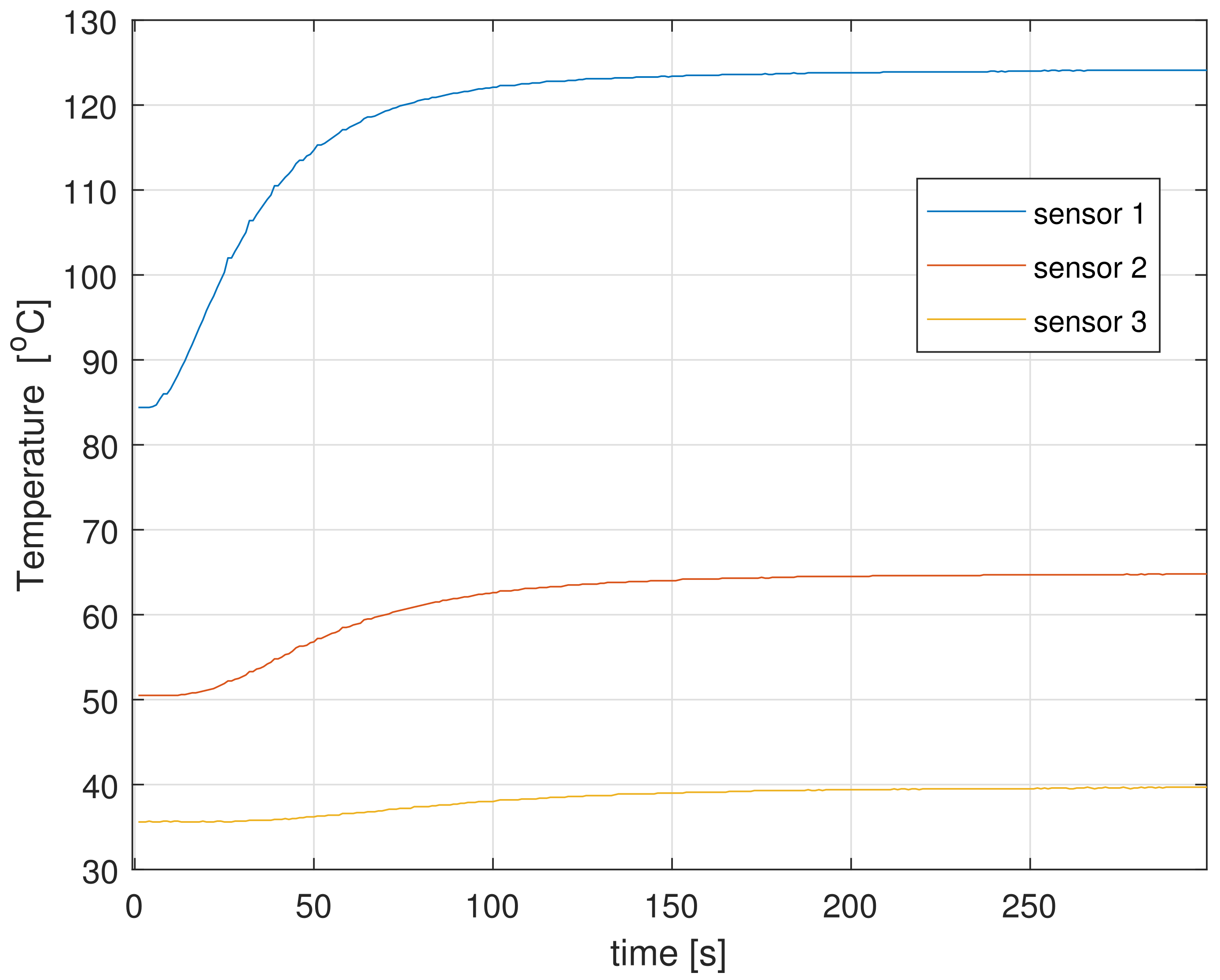
The experimental heat plant is illustrated in Figure 1. Its main part is the thin copper rod 260 [mm] long. To simplify, assume that its length equals to 1.0. Thanks to this, the location and length of the heater and RTD sensors can be described relative to 1.0. The rod is heated with the use of the electric heater long attached at the end of the rod. Temperature of rod (the output signal from the system) is measured by the miniature RTD sensors (Pt100) long attached in points 0.29, 0.50, and 0.73 of rod length. The control of the system is the standard current from range 0–20 [mA] amplified to the range 0–1.5 [A] and sent to the heater. Signals from the RTDs are read directly by analog input module in the PLC. Data from PLC are collected by SCADA application. The whole system is connected via industrial network PROFINET. The step responses measured by all sensors are presented in Figure 2.
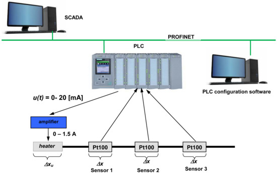
Figure 1.
The experimental system.
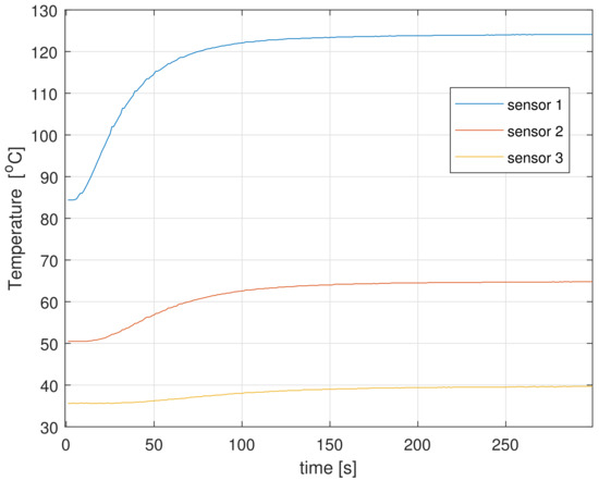
Figure 2.
The step responses from all sensors.
The fundamental time-continuous model describing the heat processes in the rod has the form of the PDE of the parabolic type with the homogeneous Neumann boundary conditions at the ends and the homogeneous initial condition. It must also take into account the heat exchange along the length of rod as well as distributed control and observation. Such an equation with integer orders of both differentiations has been discussed in many papers, such as in [34,35,36].
The FO expanding of this model is discussed with details in the papers [18,19]. In this paper, its version with interval fractional order along the length is proposed. It takes the following form:
In (8), and are known coefficients of heat conduction and heat exchange, and is a steady-state gain.
Non-integer orders and are not exactly known, and they are described by the following intervals:
where
where . This deviation can also be expressed in percents: .
where
where , or, equivalently, .
Intervals and build the vector of uncertain orders q:
All the vectors q build the space of uncertain orders Q:
Set Q can be interpreted as the rectangle in the plane stretched on the following vertices:
The center of the rectangle Q is defined by the nominal values of orders:
The dimensions of rectangle Q are determined by the size of uncertainties of and . Particularly, if one of orders is known, Q reduces to a sector, and, for both known orders, it reduces to a single point.
The interval form of orders and expands the heat transfer Equation (8) to the infinite set of equations, limited by vertices (15). Properties of each equation are determined by properties of vertex models.
In (18), is the field of state operator A, , are the first and second derivative with respect to length, and denotes the standard scalar product.
The basis of the state space is spanned by the folloiwng eigenvectors of state operator A:
3.1. The Decomposition of the Spectrum
The eigenvalues of state operator A depend only on interval order :
and, consequently, for interval , each eigenvalue expands to the interval too:
Consequently, the diagonal state operator has interval in diagonal form:
The set of all eigenvalues of state operator A build the spectrum of state operator :
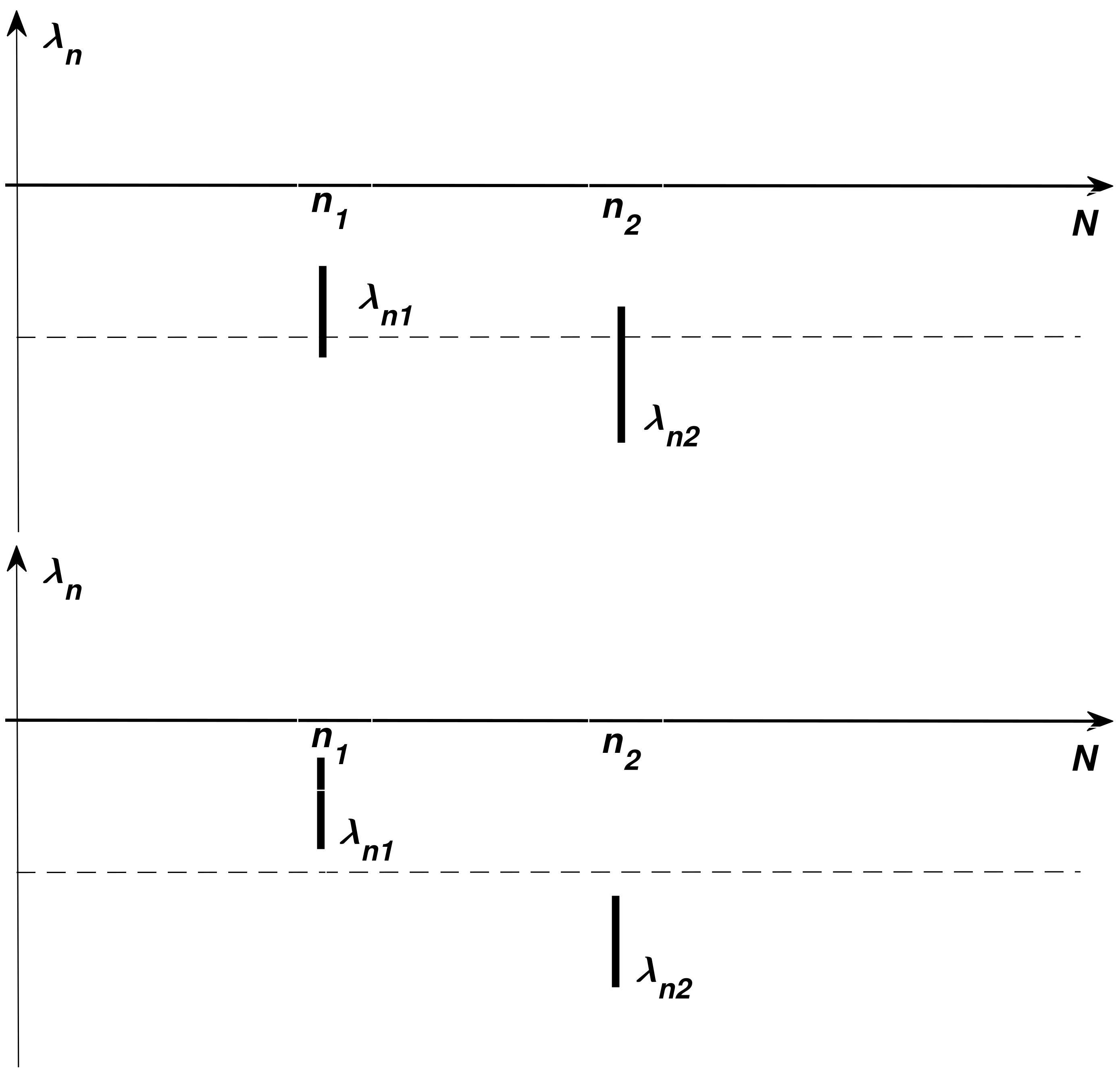
For exactly known , the spectrum contains negative, real, single, and separated eigenvalues ordered by indices n. The most poorly damped eigenvalue is called the dominant (leading) eigenvalue. This property enables easily decomposing a system into single scalar subsystems associated with particular eigenvalues. This is presented with details by [18,19]. However, for interval , the situation becomes more complicated due to particular eigenvalues expanding to intervals. This implies that eigenvalues associated with different modes can partially overlap. In such a situation, the spectrum decomposition is impossible because there exist two or more different indistinguishable eigenvalues. This situation is illustrated by Figure 3.
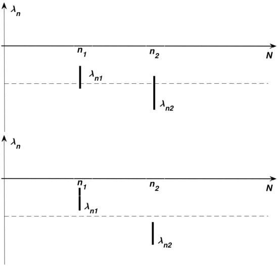
Figure 3.
The part of spectrum with eigenvalues and : overlapped in the top and non-overlapped in the bottom.
The above situation can occur if interval is too wide. Simultaneously, narrow range of uncertainty guarantees the distinguishability of the spectrum. The maximum values of and ensuring the distinguishability are described by the following propositions.
Proposition 1
(The maximum size of ensuring the distinguishability of any two eigenvalues). Consider interval spectrum (23) of the system (17). Assume that the relative uncertainty of the order β is equal to Δ.
The size ensuring the distinguishability of two eigenvalues and is expressed by the following inequality:
where
Proposition 2
(The maximum size of ensuring the distinguishability of two adjacent eigenvalues). Consider interval spectrum (23) of the system (17). Assume that the relative uncertainty of the order β is equal to Δ.
Size ensuring the distinguishability of the two adjacent eigenvalues n and is expressed by the following inequality:
where
The proof of both propositions is provided as follows:
Proof.
Consider two different interval eigenvalues and denote them by and . Assume that they are partially overlapped. This is expressed as follows:
Using logarithm function, we obtain
It is important to note that the maximum uncertainty permitted from point of view of spectrum decomposition does not depend on the value of and is determined only by location of eigenvalues, described by their indices.
Using condition (24), the maximum order N ensuring the distinguishability of all eigenvalues for given uncertainty can be obtained too. It is described by the following proposition.
Proposition 3
(The maximum dimension of the model N guaranteeing the distinguishability of the spectrum). Consider interval spectrum (23) of the system (17). Assume that the relative uncertainty of the order β is equal to Δ.
The maximum size N of the model ensuring the distinguishability of all eigenvalues meets the following inequality:
where
Proof.
Assuming and in (25) yields
Dependence (30) provides the implicit condition to estimate N. However, it can be easily applied numerically. This will be shown in the section “Simulations”.
3.2. The Input and Output Operators
Next, recall the form of input and output operators, presented, e.g., in [37]. They do not depend on interval orders of the system.
Control operator B describes the location and construction of heater. It is as follows:
where , is the shaping function of the heater:
Output operator C describes the location and size of RTDs. It is as follows:
In (36), , is the output sensor function:
Using (19) and (37) yields
It is important to note that operators B and C do not depend on uncertain orders and .
The shaping function and sensor function are piecevise constant functions.
3.3. The Step and Impulse Responses of the System with Interval Orders
If the control is the Heaviside function , then the analytical formula of step response is as follows:
where is the one-parameter Mittag-Leffler function, , , and are expressed by (20), (35), and (38), respectively. Analogically, we can compute the impulse response:
In (40), is two-parameter Mittag-Leffler function. The FO model expressed by (17)–(40) is infinitely dimensional. Of course, its practical use requires its reduction to finite dimensional form. This can be completed by truncating further modes in state Equation (17) and calculating solutions (39) or (40) as finite sums. Consequently, operators A, B, and C turn to matrices, and both time responses take the form of finite sums:
In (41) and (42), N is the dimension of finite approximation. Its value determines the accuracy of the model and can be estimated using numerical or analytical methods (see [19]).
Time responses (41) and (42) are functions of interval orders collected in the vectors (13): , . This expands them to sectors limited by the borders of intervals and :
In (43) and (44), is defined by (15). Analogically, the nominal time responses are expressed as follows:
where is the vector of nominal parameters (16).
The most obvious way to describe the sensitivity of the step response to uncertainty of the orders is to propose the sensitivity functions in the form and . However, such explicit functions are difficult to compute.
The sensitivity can also be tested using the following relative dynamic deviations :
where and
3.4. The Steady-State Response
The steady-state response of the system is as follows:
where is expressed as follows:
in (50), and are described by (35) and (38), respectively.
The responses do not depend on the order , but they are affected by the interval order only. From the point of view of the geometric interpretation of rectangle (14), (15) reduces to the section limited by the limits of the order . This is expressed as follows:
where nominal and limit values are described as follows:
and, consequently, the whole response (49) takes the form of the following interval:
The relative deviation of the steady-state response from its nominal value is the limit value of deviation expressed by (47)
4. Experiments and Simulations
The experiments were executed with the use of the laboratory stand presented in Section 1. The experimental step response was realized by changing the input signal from to of its maximum range. The step responses from all sensors are shown in Figure 2. The sample time in experiments was set to 1 s, the amount of samples was equal to , and the final time was equal to = 300 [s]. The size and location of heater and sensors are described by Table 1.

Table 1.
The size and the location of the heater and the sensors.
The analysis of sensitivity was completed using parameters of the model estimated numerically via minimization of the MSE cost function for all sensors together (see [19]—caption of Figure 6). These parameters are recalled in Table 2. The values of and are set as nominal values and .
Table 2.
The parameters of the model.
The impact of uncertainties and to model was examined numerically. The results are presented in the next subsections.
4.1. The Analysis of the Spectrum Decomposition
At the beginning, the impact of uncertainty on spectrum decomposition was tested using conditions (24), (26), and (30).
General condition (24) was examined for indices and , describing rather distant eigenvalues. The results are displayed in Table 3.
Table 3.
The maximum size allowing to distinguish between two different eigenvalues.
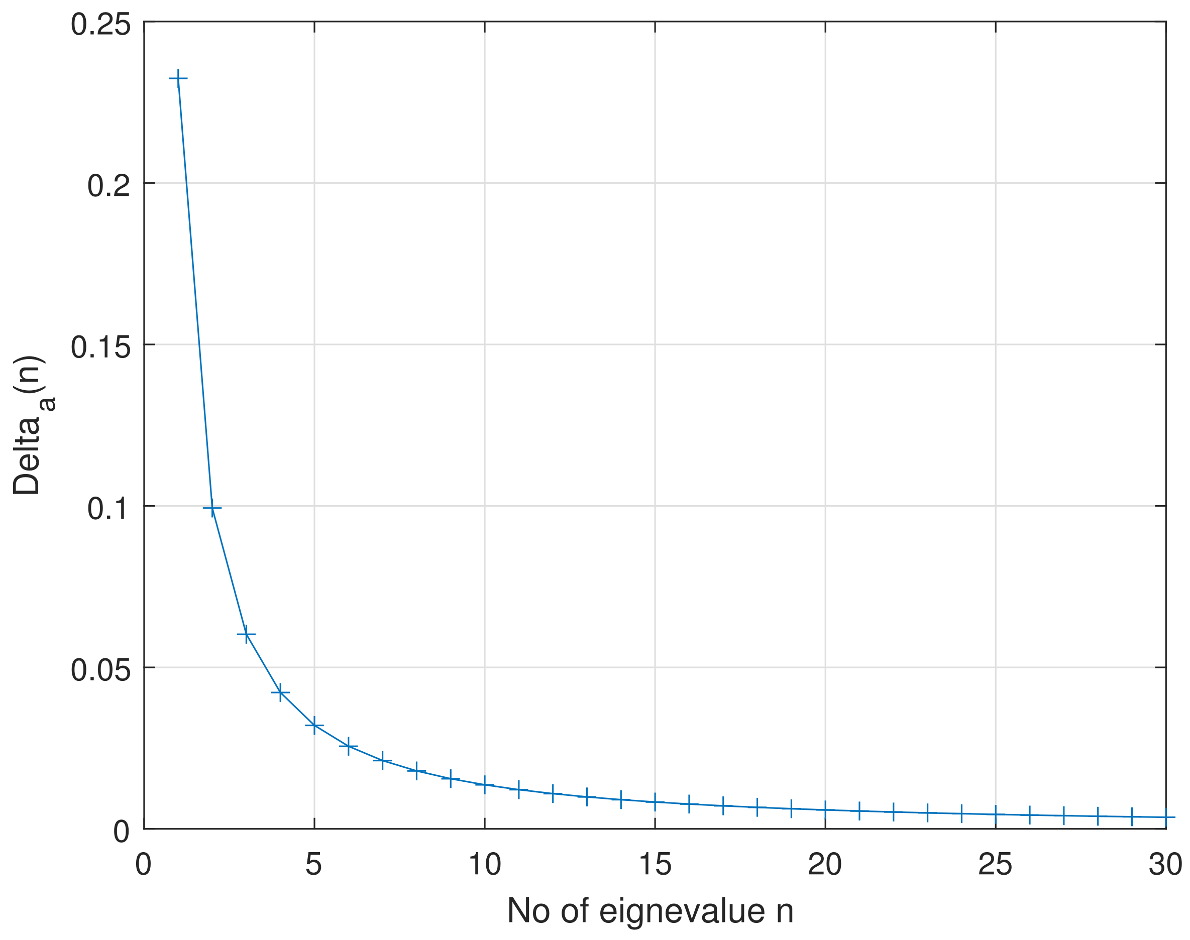
Next, the distinguishability of adjacent eigenvalues was tested using condition (26). Results are illustrated by Figure 4.
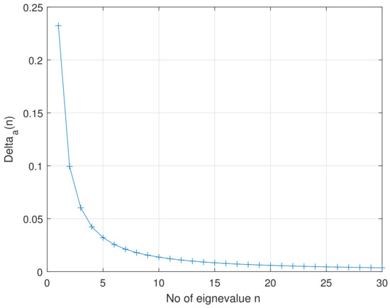
Figure 4.
The maximum uncertainty ensuring the distinguishability of two adjacent eigenvalues.
Table 3 and Figure 4 show that the distinguishability is harder to maintain for “further” eigenvalues with higher indices n.
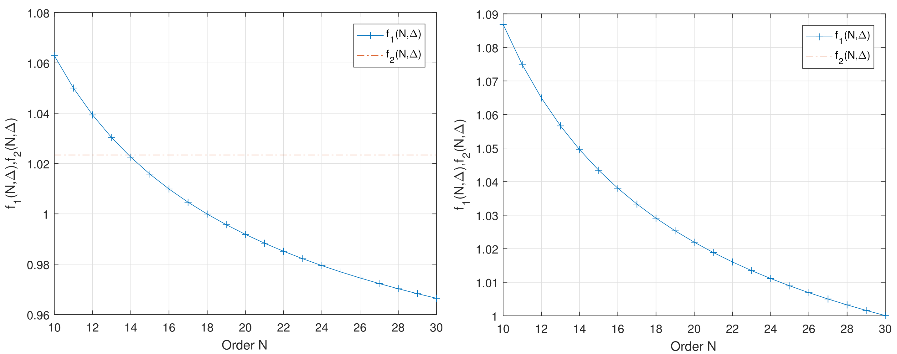
Finally, the maximum order N ensuring the distinguishability of the whole spectrum was computed using condition (30). To make it easier, denote the left and right sides of inequality (30) by and :
Using this notation, condition (30) turns to the following form:
Condition (57) was tested numerically for and . Numerical solution of inequality (57) is shown in Figure 5.
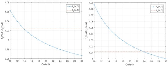
Figure 5.
The maximum N ensuring the distinguishability of all eigenvalues for (left) and (right).
The diagrams in Figure 5 show that, for , the maximum size of model is equal to 13 and, for , this maximum size is equal to 23. In general, the increase in uncertainty causes the decrease in the order of the model N, ensuring the distinguishability of the spectrum.
4.2. The Sensitivity of the Dynamics
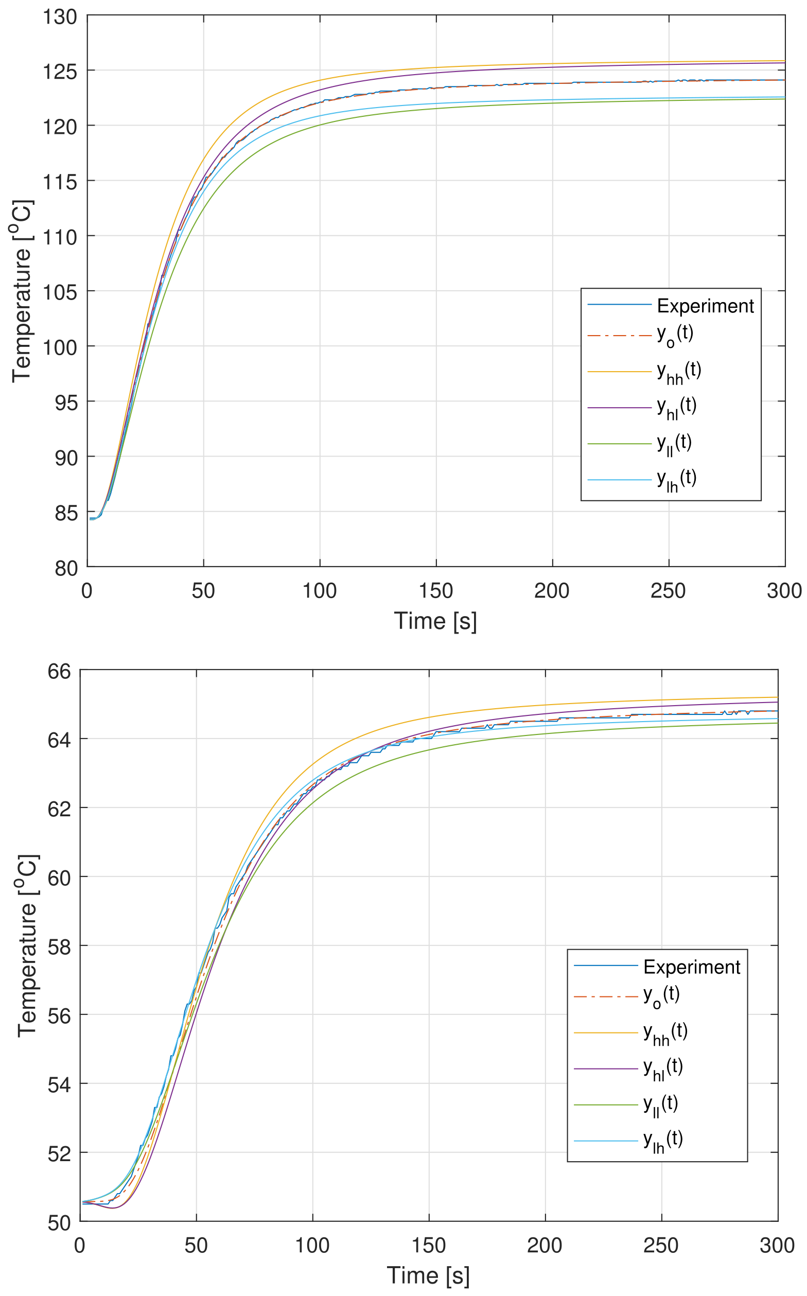
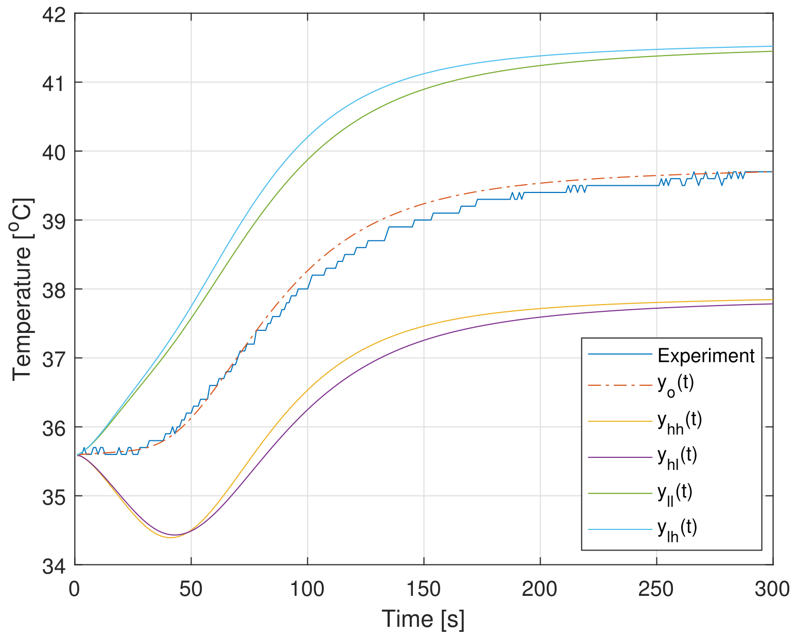
The sensitivity of the step response to uncertainties of both orders was tested using dynamic relative deviations (47) computed using data from Table 2. Both uncertainties were set to and . All vertex step responses for all outputs were compared to nominal one and experimental in Figure 6. Time trends of all deviations for all outputs of the system are shown in Figure 7.

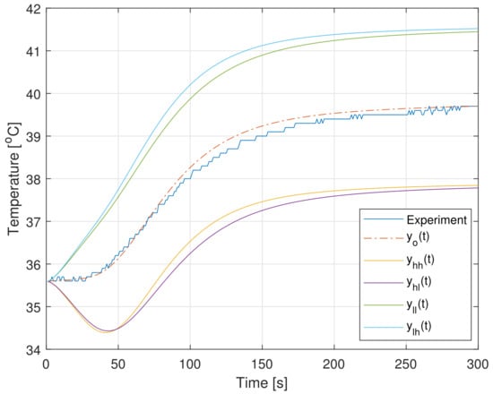
Figure 6.
The vertex step responses (43) of the model for and for outputs 1–3 (1—top; 3—bottom).
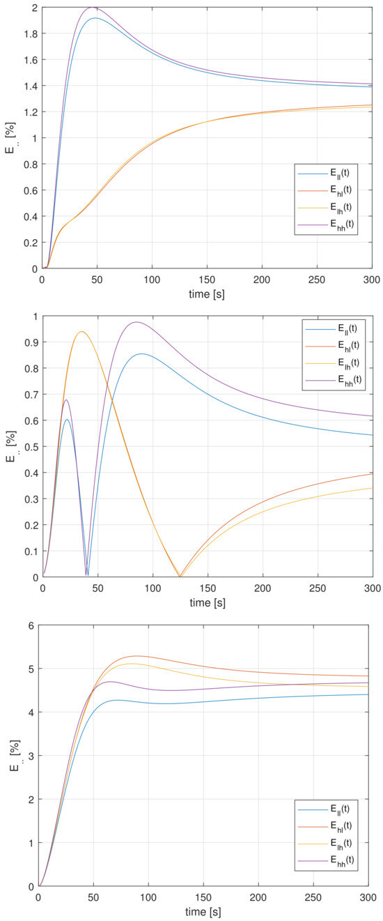
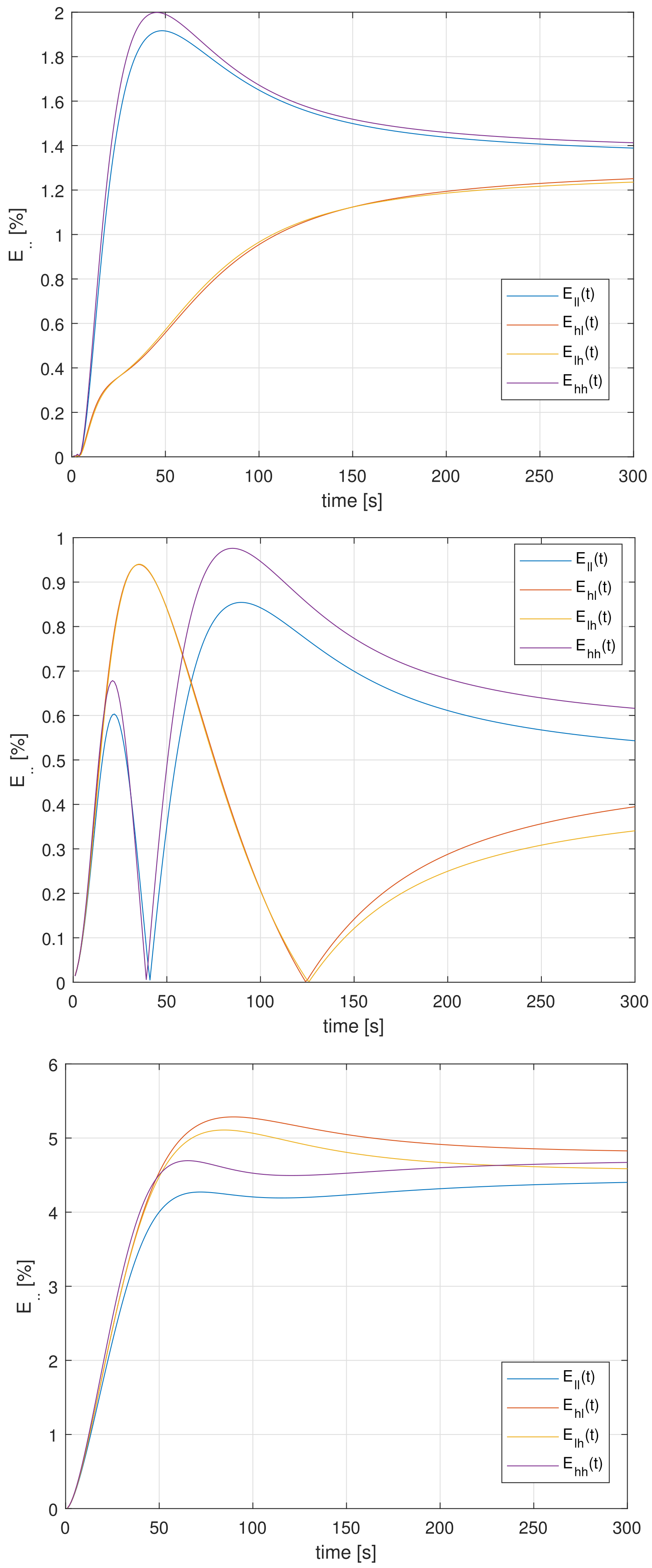
Figure 7.
The relative deviations (47) for and for outputs 1–3 (1—top; 3—bottom).
4.3. The Sensitivity of the Steady-State Response
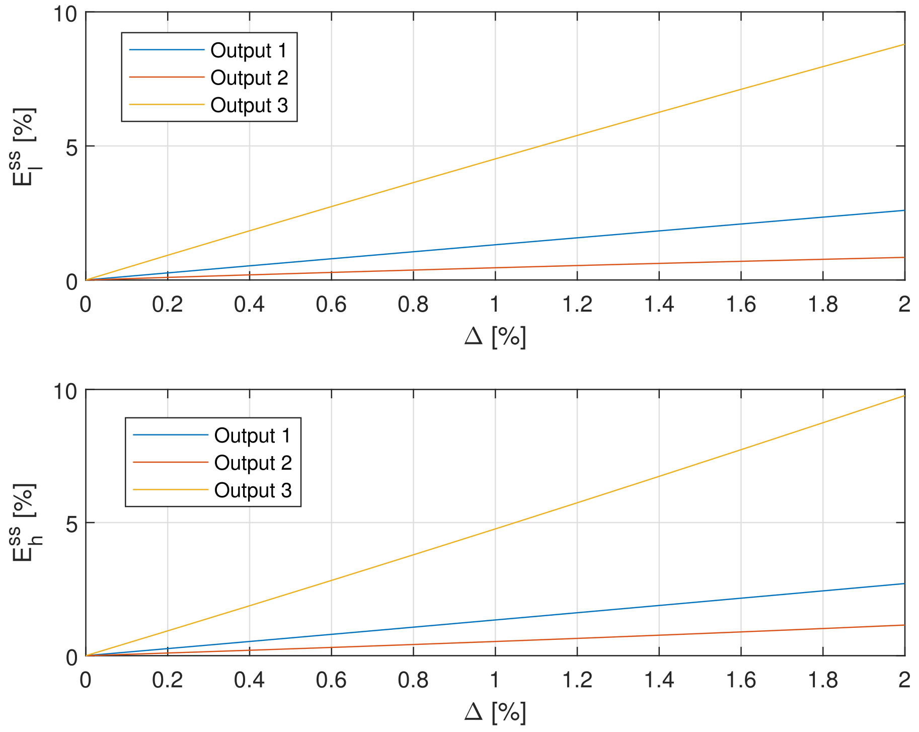
The relative steady-state error (55) was examined for small uncertainty included in the range and large uncertainty from range separately. Results are illustrated by Figure 8 and Figure 9.
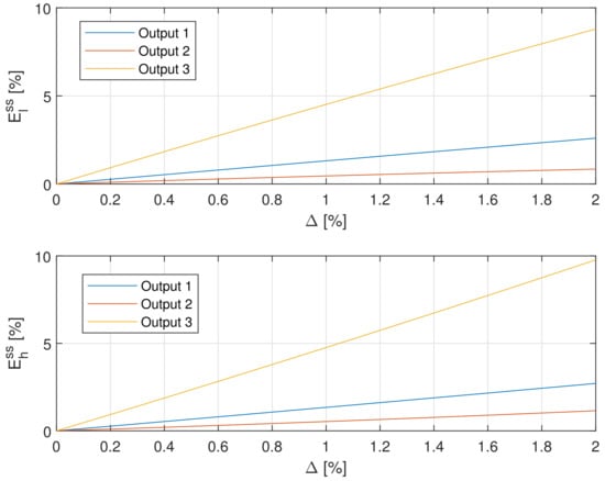
Figure 8.
The relative steady-state deviation (55) as a function of the small uncertainty for all outputs of the plant.
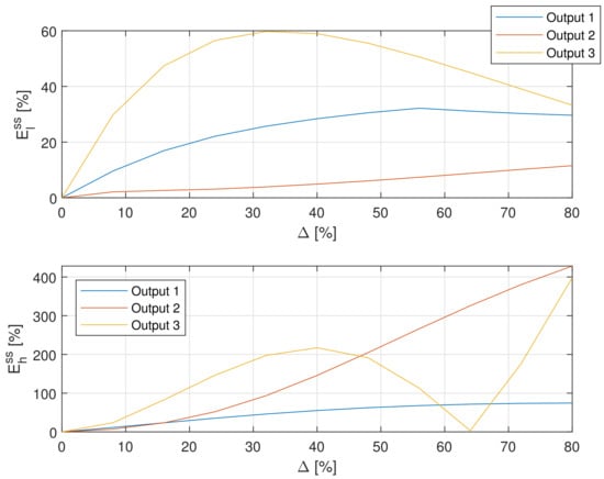
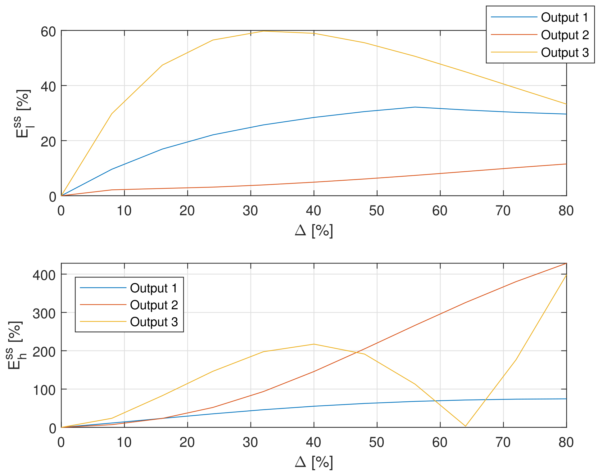
Figure 9.
The relative steady-state deviation (55) as a function of the large uncertainty for all outputs of the plant.
- The sensitivity of the steady-state response to uncertainty strongly depends on the localization of the RTD. Its is highest for the most distant sensor 3 and smaller for sensors 1 and 2.
- For small uncertainty, the deviation is approximately a linear function of , and both deviations are approximately the same.
- For larger uncertainty, the deviation is a nonlinear function of and nonlinearity is various for different outputs. Additionally, the upper deviation is much larger than lower .
5. Final Conclusions
The results presented in this paper can be summarized such that the uncertainty of both fractional orders impacts the crucial properties of the model: the distinguishability of the spectrum and the step and steady-state responses. The disturbance of order affects only the dynamics, but the disturbance of order expressed by disturbs all the considered properties of the model.
Next, the impact of disturbance is determined by its size and the place of measurement. A small disturbance (e.g., 1%) strongly disturbs output 3, furthest from the heater, and slightly interferes with the measurement at output 2, placed halfway along the length of the rod. In turn, a large disturbance (greater than 50%) disturbs output 1 the least.
Further research on the presented issues will include among others the theoretical justification of the numerical results and investigations of discrete approximated models using CFE and FOBD approximations.
Funding
This paper was supported by AGH project no 16.16.120.773.
Data Availability Statement
Data are contained within the article.
Conflicts of Interest
The author declares no conflicts of interest.
Abbreviations
| Acronym | Explanation |
| CF | Caputo–Fabrizio |
| CFE | Continuous Fraction Expansion |
| FO | Fractional Order |
| FOBD | Fractional-Order Backward Difference |
| IO | Integer Order |
| PDE | Partial Differential Equation |
| PLC | Programmable Logic Controller |
| RTD | Resistive Temperature Detector |
| SCADA | Supervisory Control and Data Acquisition |
References
- Podlubny, I. Fractional Differential Equations; Academic Press: San Diego, CA, USA, 1999. [Google Scholar]
- Dzieliński, A.; Sierociuk, D.; Sarwas, G. Some applications of fractional order calculus. Bull. Pol. Acad. Sci. Tech. Sci. 2010, 58, 583–592. [Google Scholar] [CrossRef]
- Caponetto, R.; Dongola, G.; Fortuna, L.; Petras, I. Fractional Order Systems: Modeling and Control Applications. In World Scientific Series on Nonlinear Science; Chua, L.O., Ed.; University of California: Berkeley, CA, USA, 2010; pp. 1–178. [Google Scholar]
- Das, S. Functional Fractional Calculus for System Identification and Controls; Springer: Berlin/Heilderberg, Germany, 2010. [Google Scholar]
- Gal, C.; Warma, M. Elliptic and parabolic equations with fractional diffusion and dynamic boundary conditions. Evol. Equ. Control Theory 2016, 5, 61–103. [Google Scholar]
- Popescu, E. On the fractional Cauchy problem associated with a Feller semigroup. Math. Rep. 2010, 12, 181–188. [Google Scholar]
- Sierociuk, D.; Skovranek, T.; Macias, M.; Podlubny, I.; Petras, I.; Dzielinski, A.; Ziubinski, P. Diffusion process modeling by using fractional-order models. Appl. Math. Comput. 2015, 257, 2–11. [Google Scholar] [CrossRef]
- Gómez, J.F.; Torres, L.; Escobar, R.F. Fractional Derivatives with Mittag-Leffler Kernel. Trends and Applications in Science and Engineering. In Studies in Systems, Decision and Control; Kacprzyk, J., Ed.; Springer: Cham, Switzerland, 2019; Volume 194, pp. 1–339. [Google Scholar]
- Boudaoui, A.; El hadj Moussa, Y.; Hammouch, Z.; Ullah, S. A fractional-order model describing the dynamics of the novel coronavirus (COVID-19) with nonsingular kernel. Chaos Solitons Fractals 2021, 146, 1–11. [Google Scholar] [CrossRef] [PubMed]
- Farman, M.; Akgül, A.; Askar, S.; Botmart, T.; Ahmad, A.; Ahmad, H. Modeling and analysis of fractional order Zika model. AIMS Math. 2022, 7, 3912–3938. [Google Scholar] [CrossRef]
- Dlugosz, M.; Skruch, P. The application of fractional-order models for thermal process modelling inside buildings. J. Build. Phys. 2015, 1, 1–13. [Google Scholar] [CrossRef]
- Ryms, M.; Tesch, K.; Lewandowski, W. The use of thermal imaging camera to estimate velocity profiles based on temperature distribution in a free convection boundary layer. Int. J. Heat Mass Transf. 2021, 165, 120686. [Google Scholar] [CrossRef]
- Wu, S.Y.; Yuan, X.F.; Li, Y.R. Two non-dimensional exergy transfer performance parameters of heat exchanger. Int. J. Exergy 2010, 7, 130–145. [Google Scholar] [CrossRef]
- Khan, H.; Shah, R.; Kumam, P.; Arif, M. Analytical Solutions of Fractional-Order Heat and Wave Equations by the Natural Transform Decomposition Method. Entropy 2019, 21, 597. [Google Scholar] [CrossRef] [PubMed]
- Olsen-Kettle, L. Numerical Solution of Partial Differential Equations; The University of Queensland: St. Lucia, QLD, Australia, 2011. [Google Scholar]
- Al-Omari, S.K. A fractional Fourier integral operator and its extension to classes of function spaces. Adv. Differ. Equ. 2018, 1, 1–9. [Google Scholar] [CrossRef]
- Xue, W.; Wang, Y.; Liang, Y.; Wang, T.; Ren, B. Efficient hydraulic and thermal simulation model of the multi-phase natural gas production system with variable speed compressors. Appl. Therm. Eng. 2024, 242, 122411. [Google Scholar] [CrossRef]
- Oprzędkiewicz, K.; Gawin, E.; Mitkowski, W. Modeling heat distribution with the use of a non-integer order, state space model. Int. J. Appl. Math. Comput. Sci. 2016, 26, 749–756. [Google Scholar] [CrossRef]
- Oprzędkiewicz, K.; Gawin, E.; Mitkowski, W. Parameter identification for non integer order, state space models of heat plant. In Proceedings of the MMAR 2016: 21th international conference on Methods and Models in Automation and Robotics, Międzyzdroje, Poland, 29 August–1 September 2016; pp. 184–188. [Google Scholar]
- Oprzedkiewicz, K.; Stanislawski, R.; Gawin, E.; Mitkowski, W. A new algorithm for a CFE approximated solution of a discrete-time non integer-order state equation. Bull. Pol. Acad. Sci. Tech. Sci. 2017, 65, 429–437. [Google Scholar]
- Oprzędkiewicz, K.; Mitkowski, W.; Gawin, E. An accuracy estimation for a non integer order, discrete, state space model of heat transfer process. In Proceedings of the Automation 2017: Innovations in Automation, Robotics and Measurment Techniques, Warsaw, Poland, 15–17 March 2017; pp. 86–98. [Google Scholar]
- Oprzędkiewicz, K.; Mitkowski, W.; Gawin, E.; Dziedzic, K. The Caputo vs. Caputo-Fabrizio operators in modeling of heat transfer process. Bull. Pol. Acad. Sci. Tech. Sci. 2018, 66, 501–507. [Google Scholar]
- Oprzędkiewicz, K.; Gawin, E. The practical stability of the discrete, fractional order, state space model of the heat transfer process. Arch. Control Sci. 2018, 28, 463–482. [Google Scholar] [CrossRef]
- Oprzędkiewicz, K.; Mitkowski, W. A memory efficient non integer order discrete time state space model of a heat transfer process. Int. J. Appl. Math. Comput. Sci. 2018, 28, 649–659. [Google Scholar] [CrossRef]
- Oprzędkiewicz, K. Non integer order, state space model of heat transfer process using Atangana-Baleanu operator. Bull. Pol. Acad. Sci. Tech. Sci. 2020, 68, 43–50. [Google Scholar] [CrossRef]
- Oprzędkiewicz, K. Fractional order, discrete model of heat transfer process using time and spatial Grünwald-Letnikov operator. Bull. Pol. Acad. Sci. Tech. Sci. 2021, 69, 1–10. [Google Scholar] [CrossRef]
- Oprzędkiewicz, K.; Mitkowski, W.; Rosol, M. Fractional order model of the two dimensional heat transfer process. Energies 2021, 14, 6371. [Google Scholar] [CrossRef]
- Oprzędkiewicz, K.; Mitkowski, W.; Rosol, M. Fractional order, state space model of the temperature field in the PCB plate. Acta Mech. Autom. 2023, 17, 180–187. [Google Scholar] [CrossRef]
- Kaczorek, T. Stability of interval positive fractional discrete-time systems. Int. J. Appl. Math. Comput. Sci. 2018, 28, 451–456. [Google Scholar] [CrossRef]
- Kaczorek, T. Singular fractional linear systems and electrical circuits. Int. J. Appl. Math. Comput. Sci. 2011, 21, 379–384. [Google Scholar] [CrossRef]
- Kaczorek, T.; Rogowski, K. Fractional Linear Systems and Electrical Circuits; Bialystok University of Technology: Bialystok, Poland, 2014. [Google Scholar]
- Bandyopadhyay, B.; Kamal, S. Solution, Stability and Realization of Fractional Order Differential Equation. In Stabilization and Control of Fractional Order Systems: A Sliding Mode Approach; Lecture Notes in Electrical Engineering; Springer: Cham, Switzerland, 2015; Volume 317, pp. 55–90. [Google Scholar]
- Mozyrska, D.; Girejko, E.; Wyrwas, M. Comparison of h-difference fractional operators. In Advances in the Theory and Applications of Non-integer Order Systems; Mitkowski, W., Kacprzyk, J., Baranowski, J., Eds.; Springer: Cham, Switzerland, 2013; pp. 1–178. [Google Scholar]
- Oprzędkiewicz, K. The interval parabolic system. Arch. Control Sci. 2003, 13, 415–430. [Google Scholar]
- Oprzędkiewicz, K. A controllability problem for a class of uncertain parameters linear dynamic systems. Arch. Control Sci. 2004, 14, 85–100. [Google Scholar]
- Oprzędkiewicz, K. An observability problem for a class of uncertain-parameter linear dynamic systems. Int. J. Appl. Math. Comput. Sci. 2005, 15, 331–338. [Google Scholar]
- Oprzędkiewicz, K. Positivity problem for the one dimensional heat transfer process. ISA Trans. 2021, 112, 281–291. [Google Scholar] [CrossRef] [PubMed]

Disclaimer/Publisher’s Note: The statements, opinions and data contained in all publications are solely those of the individual author(s) and contributor(s) and not of MDPI and/or the editor(s). MDPI and/or the editor(s) disclaim responsibility for any injury to people or property resulting from any ideas, methods, instructions or products referred to in the content. |
© 2024 by the author. Licensee MDPI, Basel, Switzerland. This article is an open access article distributed under the terms and conditions of the Creative Commons Attribution (CC BY) license (https://creativecommons.org/licenses/by/4.0/).