1. Introduction
The results of many authors have been indicating for years that the FO calculus serves as a very convenient tool to describe many physical, biological, and social processes.
Fundamental examples of such models were provided, e.g., in [
1,
2] (thermal processes in a one-dimensional beam), ref. [
3] (FO models of chaotic systems and Ionic Polymer Metal Composites), and [
4]. Non-integer-order models of diffusion processes were presented, for example, in [
5,
6,
7]. The results of presenting the use of a new Atangana–Baleanu operator were provided in [
8]. They covered among others the FO blood alcohol model, the Christov diffusion equation, and the fractional advection–dispersion equation for groundwater transport processes.
Recently, FO models have been applied to describe the spread of diseases, such as FO models of the dynamics of COVID-19 using the Caputo–Fabrizio operator presented by [
9] or the model of the transmission of the Zika virus using the Atangana–Baleanu operator proposed by [
10].
Models of temperature fields have been considered by many authors, e.g., [
11,
12]. New, dimensionless cost functions describing the exergy of a heat exchanger were proposed in [
13]. The two-dimensional IO heat transfer equation was analytically solved in [
14]. The numerical methods of the solution of PDEs were provided by various authors, e.g., in [
15]. Fractional Fourier integral operators were analyzed in [
16]. Most of the known results described only steady-state temperature fields while omitting their dynamics.
The recent results from the area of the modeling of the thermal processes in the industry cover, among others, the modeling of the thermal processes in gas distribution systems [
17].
FO models of one-dimensional heat transfer in the state space have been proposed in many previous papers of authors from the years 2016–2018 and 2020 [
18,
19,
20,
21,
22,
23,
24,
25]. In the proposed models, different FO operators were employed. There were Grünwald–Letnikov, Caputo, Caputo–Fabrizio, and Atangana–Baleanu, as well as discrete operators CFE and FOBD. Each proposed model has been thoroughly justified theoretically and experimentally. The accuracy of each FO model regarding the square cost function was better than its IO analogue.
The sensitivity of the FO model to the uncertainty of the coefficients describing the heat conduction and heat exchange was considered in [
26]. In this paper, the uncertainty of the fractional orders was not considered. Such an analysis is provided in this paper.
The papers [
27,
28] presented the two-dimensional generalization of the FO models proposed previously.
This article presents the generalization of the model provided in [
22] to the case when both fractional orders are described by intervals. Such an approach should better describe reality because the fractional orders are difficult to estimate in contrast to the parameters describing heat transfer and heat conduction. Based on the knowledge of the author, such a model has not been proposed yet. The interval fractional-order system was considered, e.g., by [
29], but this paper deals with the interval state operator and known interval order of the derivative in relation to time.
The organization of the paper is as follows. The preliminaries provide the basic ideas from fractional calculus that are necessary to explain the main results. Next, the experimental system and its FO model with interval orders are proposed and analyzed. Finally, the experimental validation of the theoretical results is shown.
2. Preliminaries
Preliminaries will start with defining of the non-integer-order integro-differential operator (see, e.g., [
1,
4,
30,
31]).
Definition 1 (The basic non-integer-order operator).
The fractional-order integro-differential operator is defined as follows:where a and t are time limits for operator computing and is the fractional order of the operation. In (
1), the positive value of
denotes the derivation, and its negative value describes the integration. Simultaneously, for integer values of
, this definition describes IO derivation or integration. The next significant difference is that a fractional derivative is computed on an interval
and not at a point.
Next, recall an idea of complete Gamma Euler function (see, e.g., [
31]):
Definition 2 (The complete Gamma function).
Function (2) is the generalization of factorial to real numbers.
Next, recall the two-parameter Mittag-Leffler function. It is a non-integer-order generalization of exponential function and plays a crucial role in the solution of an FO state equation. It is defined as follows:
Definition 3 (The two-parameter Mittag-Leffler function).
For , the two-parameter function reduces to the one-parameter Mittag-Leffler function:
Definition 4 (The one-parameter Mittag-Leffler function).
The FO operator (
1) can be expressed by three fundamental definitions, formulated by Grünwald and Letnikov (GL definition), Riemann and Liouville (RL definition), and Caputo (C definition). Relationships between Caputo and Riemann–Liouville and between Riemann–Liouville and Grünwald–Letnikov operators are proven, for example, in [
4,
32]. Discrete versions of these operators are deeply analyzed by [
33]. The C definition has intuitive interpretation of an initial condition as well as Laplace transform. Additionally, its value from a constant equals to zero, in contrast to, e.g., RL definition. That is why the C definition will be applied in this paper. It is provided below.
Definition 5 (The Caputo definition of the FO operator).
In (
5),
V describes a limiter of the non-integer order
. For
, the order of operation lies in the range
, and the definition of (
5) takes the form
Finally, a fractional linear state equation employing the C definition should be recalled. It is as follows:
where
denotes the fractional order of the state equation,
,
, and
denote the state, control, and output vectors, respectively, and
are the state, control, and output matrices.
3. The Experimental System and Its Model with Fractional Interval Orders
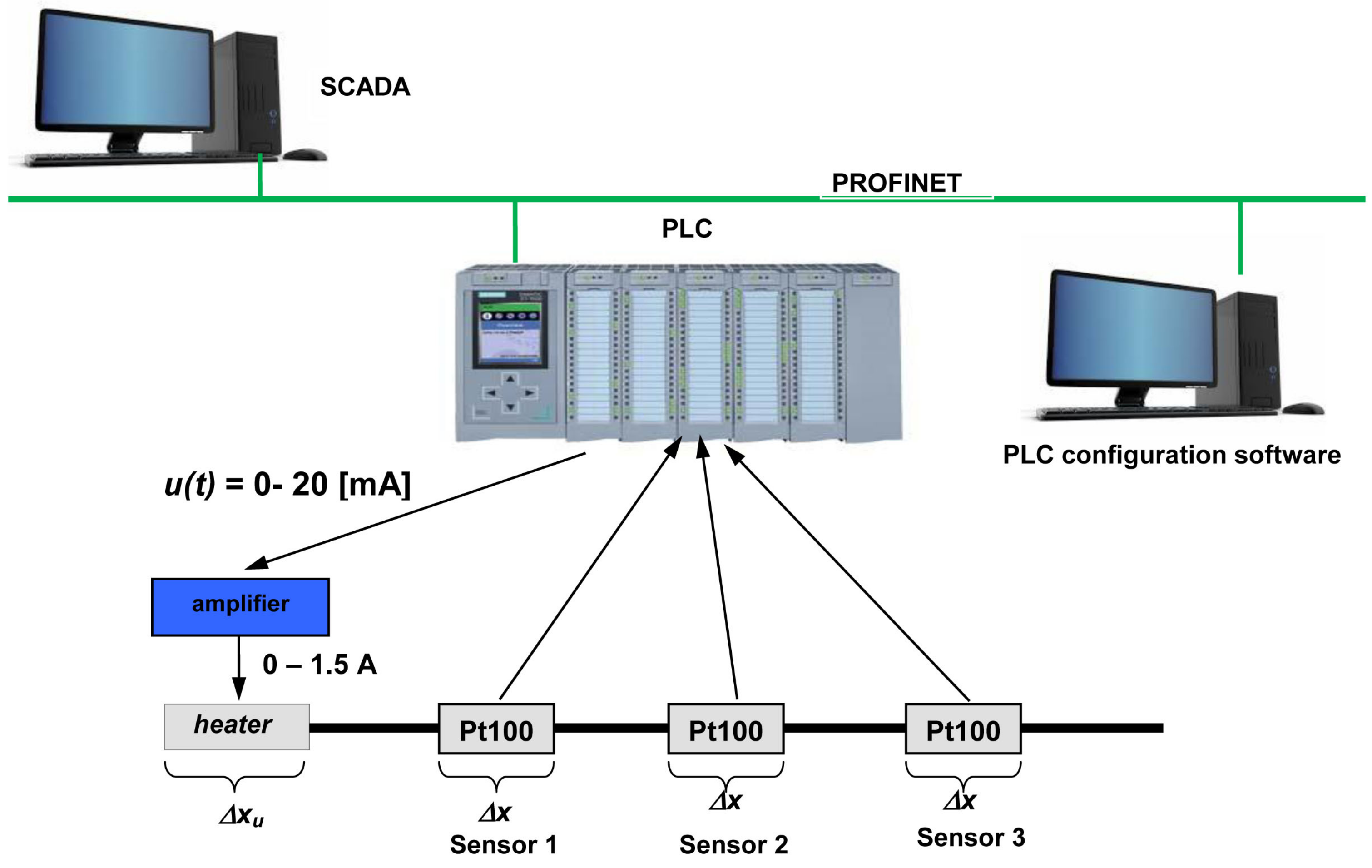
The experimental heat plant is illustrated in
Figure 1. Its main part is the thin copper rod 260 [mm] long. To simplify, assume that its length equals to 1.0. Thanks to this, the location and length of the heater and RTD sensors can be described relative to 1.0. The rod is heated with the use of the electric heater
long attached at the end of the rod. Temperature of rod (the output signal from the system) is measured by the miniature RTD sensors (Pt100) long
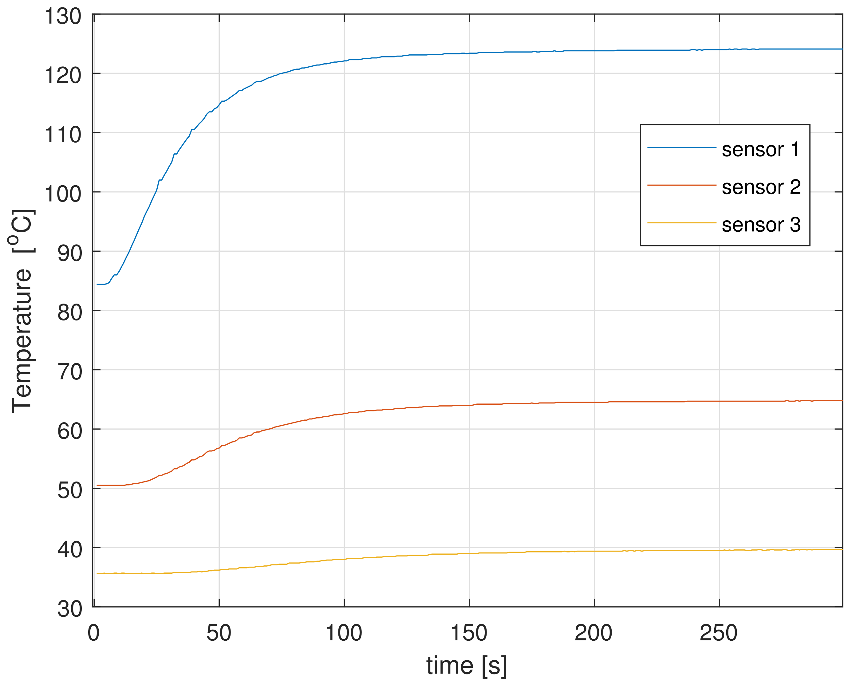
attached in points 0.29, 0.50, and 0.73 of rod length. The control of the system is the standard current from range 0–20 [mA] amplified to the range 0–1.5 [A] and sent to the heater. Signals from the RTDs are read directly by analog input module in the PLC. Data from PLC are collected by SCADA application. The whole system is connected via industrial network PROFINET. The step responses measured by all sensors are presented in
Figure 2.
The fundamental time-continuous model describing the heat processes in the rod has the form of the PDE of the parabolic type with the homogeneous Neumann boundary conditions at the ends and the homogeneous initial condition. It must also take into account the heat exchange along the length of rod as well as distributed control and observation. Such an equation with integer orders of both differentiations has been discussed in many papers, such as in [
34,
35,
36].
The FO expanding of this model is discussed with details in the papers [
18,
19]. In this paper, its version with interval fractional order along the length is proposed. It takes the following form:
In (
8),
and
are known coefficients of heat conduction and heat exchange, and
is a steady-state gain.
Non-integer orders
and
are not exactly known, and they are described by the following intervals:
where
where
. This deviation can also be expressed in percents:
.
where
where
, or, equivalently,
.
Intervals
and
build the vector of uncertain orders
q:
All the vectors
q build the space of uncertain orders
Q:
Set
Q can be interpreted as the rectangle in the
plane stretched on the following vertices:
The center of the rectangle
Q is defined by the nominal values of orders:
The dimensions of rectangle Q are determined by the size of uncertainties of and . Particularly, if one of orders is known, Q reduces to a sector, and, for both known orders, it reduces to a single point.
The interval form of orders
and
expands the heat transfer Equation (
8) to the infinite set of equations, limited by vertices (
15). Properties of each equation are determined by properties of vertex models.
Differential Equation (
8) can be expressed as follows:
where
In (
18),
is the field of state operator
A,
,
are the first and second derivative with respect to length, and
denotes the standard scalar product.
The basis of the state space is spanned by the folloiwng eigenvectors of state operator
A:
3.1. The Decomposition of the Spectrum
The eigenvalues of state operator
A depend only on interval order
:
and, consequently, for interval
, each eigenvalue expands to the interval too:
Consequently, the diagonal state operator has interval in diagonal form:
The set of all eigenvalues of state operator
A build the spectrum of state operator
:
For exactly known
, the spectrum contains negative, real, single, and separated eigenvalues ordered by indices
n. The most poorly damped eigenvalue
is called the dominant (leading) eigenvalue. This property enables easily decomposing a system into single scalar subsystems associated with particular eigenvalues. This is presented with details by [
18,
19]. However, for interval
, the situation becomes more complicated due to particular eigenvalues expanding to intervals. This implies that eigenvalues associated with different modes can partially overlap. In such a situation, the spectrum decomposition is impossible because there exist two or more different indistinguishable eigenvalues. This situation is illustrated by
Figure 3.
The above situation can occur if interval is too wide. Simultaneously, narrow range of uncertainty guarantees the distinguishability of the spectrum. The maximum values of and ensuring the distinguishability are described by the following propositions.
Proposition 1 (The maximum size of
ensuring the distinguishability of any two eigenvalues).
Consider interval spectrum (23) of the system (17). Assume that the relative uncertainty of the order β is equal to Δ.The size ensuring the distinguishability of two eigenvalues and is expressed by the following inequality:where Proposition 2 (The maximum size of
ensuring the distinguishability of two adjacent eigenvalues).
Consider interval spectrum (23) of the system (17). Assume that the relative uncertainty of the order β is equal to Δ.Size ensuring the distinguishability of the two adjacent eigenvalues n and is expressed by the following inequality:where The proof of both propositions is provided as follows:
Proof. Consider two different interval eigenvalues and denote them by
and
. Assume that they are partially overlapped. This is expressed as follows:
Using logarithm function, we obtain
After some elementary transformations, we obtain (
24) and the proof is completed. Assuming
and
directly provides condition (
26). □
It is important to note that the maximum uncertainty permitted from point of view of spectrum decomposition does not depend on the value of and is determined only by location of eigenvalues, described by their indices.
Using condition (
24), the maximum order
N ensuring the distinguishability of all eigenvalues for given uncertainty
can be obtained too. It is described by the following proposition.
Proposition 3 (The maximum dimension of the model
N guaranteeing the distinguishability of the spectrum).
Consider interval spectrum (23) of the system (17). Assume that the relative uncertainty of the order β is equal to Δ.The maximum size N of the model ensuring the distinguishability of all eigenvalues meets the following inequality:where Proof. Computing
L from (
24), we obtain
Assuming
and
in (
25) yields
From (
32), we obtain (
30), and the proof is completed. □
Dependence (
30) provides the implicit condition to estimate
N. However, it can be easily applied numerically. This will be shown in the section “Simulations”.
3.2. The Input and Output Operators
Next, recall the form of input and output operators, presented, e.g., in [
37]. They do not depend on interval orders of the system.
Control operator
B describes the location and construction of heater. It is as follows:
where
,
is the shaping function of the heater:
According to (
19) and (
34), each element
takes the following form:
Output operator
C describes the location and size of RTDs. It is as follows:
In (
36),
,
is the output sensor function:
Using (
19) and (
37) yields
It is important to note that operators
B and
C do not depend on uncertain orders
and
.
The shaping function and sensor function are piecevise constant functions.
3.3. The Step and Impulse Responses of the System with Interval Orders
If the control is the Heaviside function
, then the analytical formula of step response is as follows:
where
is the one-parameter Mittag-Leffler function,
,
, and
are expressed by (
20), (
35), and (
38), respectively. Analogically, we can compute the impulse response:
In (
40),
is two-parameter Mittag-Leffler function. The FO model expressed by (
17)–(
40) is infinitely dimensional. Of course, its practical use requires its reduction to finite dimensional form. This can be completed by truncating further modes in state Equation (
17) and calculating solutions (
39) or (
40) as finite sums. Consequently, operators
A,
B, and
C turn to matrices, and both time responses take the form of finite sums:
In (
41) and (
42),
N is the dimension of finite approximation. Its value determines the accuracy of the model and can be estimated using numerical or analytical methods (see [
19]).
Time responses (
41) and (
42) are functions of interval orders collected in the vectors (
13):
,
. This expands them to sectors limited by the borders of intervals
and
:
In (
43) and (
44),
is defined by (
15). Analogically, the nominal time responses are expressed as follows:
where
is the vector of nominal parameters (
16).
The most obvious way to describe the sensitivity of the step response to uncertainty of the orders is to propose the sensitivity functions in the form and . However, such explicit functions are difficult to compute.
The sensitivity can also be tested using the following relative dynamic deviations
:
where
and
3.4. The Steady-State Response
The steady-state response of the system is as follows:
where
is expressed as follows:
in (
50),
and
are described by (
35) and (
38), respectively.
The responses
do not depend on the order
, but they are affected by the interval order
only. From the point of view of the geometric interpretation of rectangle (
14), (
15) reduces to the section limited by the limits of the order
. This is expressed as follows:
where nominal and limit values are described as follows:
and, consequently, the whole response (
49) takes the form of the following interval:
The relative deviation
of the steady-state response from its nominal value is the limit value of deviation
expressed by (
47)
Using (
53), deviation (
54) is expressed as
4. Experiments and Simulations
The experiments were executed with the use of the laboratory stand presented in
Section 1. The experimental step response was realized by changing the input signal from
to
of its maximum range. The step responses from all sensors are shown in
Figure 2. The sample time in experiments was set to 1 s, the amount of samples was equal to
, and the final time was equal to
= 300 [s]. The size and location of heater and sensors are described by
Table 1.
The analysis of sensitivity was completed using parameters of the model estimated numerically via minimization of the MSE cost function for all sensors together (see [
19]—caption of Figure 6). These parameters are recalled in
Table 2. The values of
and
are set as nominal values
and
.
The impact of uncertainties and to model was examined numerically. The results are presented in the next subsections.
4.1. The Analysis of the Spectrum Decomposition
At the beginning, the impact of uncertainty
on spectrum decomposition was tested using conditions (
24), (
26), and (
30).
General condition (
24) was examined for indices
and
, describing rather distant eigenvalues. The results are displayed in
Table 3.
Next, the distinguishability of adjacent eigenvalues was tested using condition (
26). Results are illustrated by
Figure 4.
Table 3 and
Figure 4 show that the distinguishability is harder to maintain for “further” eigenvalues with higher indices
n.
Finally, the maximum order
N ensuring the distinguishability of the whole spectrum was computed using condition (
30). To make it easier, denote the left and right sides of inequality (
30) by
and
:
Using this notation, condition (
30) turns to the following form:
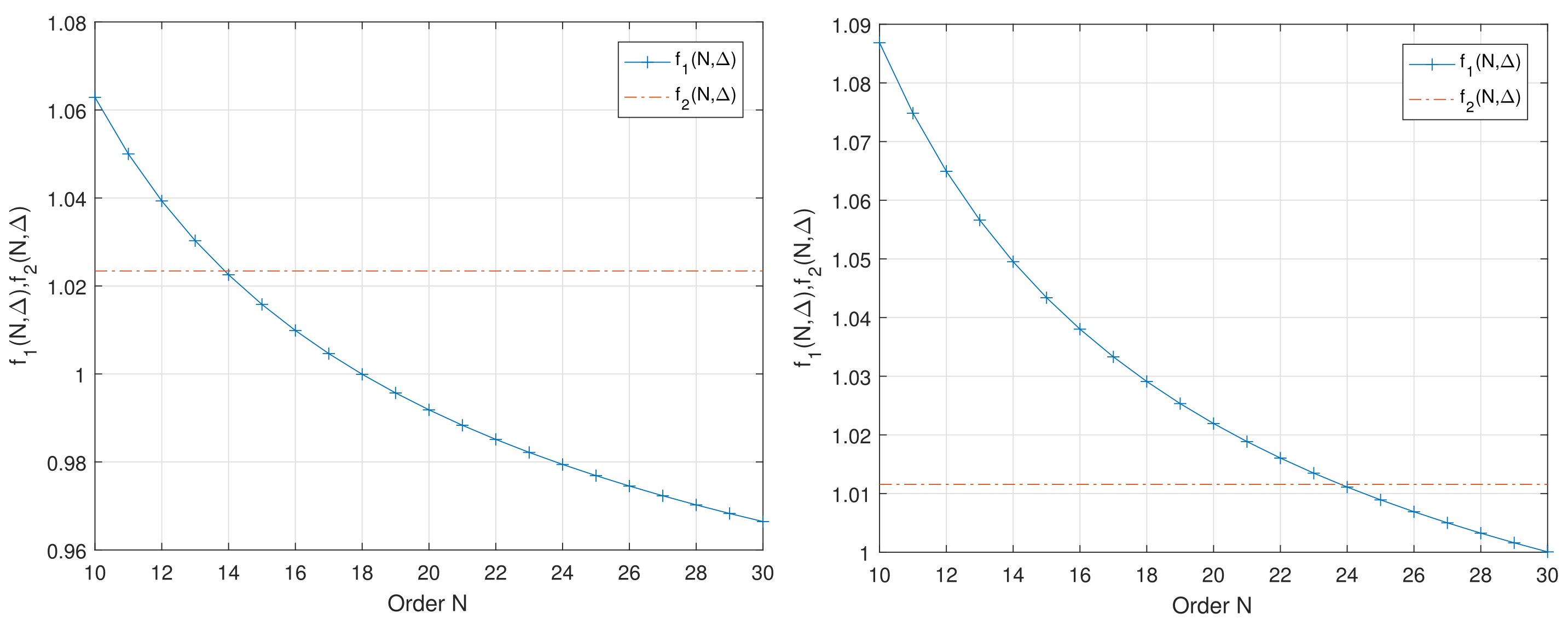
Condition (
57) was tested numerically for
and
. Numerical solution of inequality (
57) is shown in
Figure 5.
The diagrams in
Figure 5 show that, for
, the maximum size of model is equal to 13 and, for
, this maximum size is equal to 23. In general, the increase in uncertainty
causes the decrease in the order of the model
N, ensuring the distinguishability of the spectrum.
4.2. The Sensitivity of the Dynamics
The sensitivity of the step response to uncertainties of both orders was tested using dynamic relative deviations (
47) computed using data from
Table 2. Both uncertainties were set to
and
. All vertex step responses for all outputs were compared to nominal one and experimental in
Figure 6. Time trends of all deviations for all outputs of the system
are shown in
Figure 7.
In
Figure 6 and
Figure 7, it can be noted that the shape and maximum of deviation (
47) strongly depend on the observed output. It is smallest for sensor No. 2 and largest for sensor No. 3. Next, the impact of the uncertainty
goes to zero for
.
4.3. The Sensitivity of the Steady-State Response
The relative steady-state error (
55) was examined for small uncertainty included in the range
and large uncertainty from range
separately. Results are illustrated by
Figure 8 and
Figure 9.
The sensitivity of the steady-state response to uncertainty strongly depends on the localization of the RTD. Its is highest for the most distant sensor 3 and smaller for sensors 1 and 2.
For small uncertainty, the deviation is approximately a linear function of , and both deviations are approximately the same.
For larger uncertainty, the deviation is a nonlinear function of and nonlinearity is various for different outputs. Additionally, the upper deviation is much larger than lower .
5. Final Conclusions
The results presented in this paper can be summarized such that the uncertainty of both fractional orders impacts the crucial properties of the model: the distinguishability of the spectrum and the step and steady-state responses. The disturbance of order affects only the dynamics, but the disturbance of order expressed by disturbs all the considered properties of the model.
Next, the impact of disturbance is determined by its size and the place of measurement. A small disturbance (e.g., 1%) strongly disturbs output 3, furthest from the heater, and slightly interferes with the measurement at output 2, placed halfway along the length of the rod. In turn, a large disturbance (greater than 50%) disturbs output 1 the least.
Further research on the presented issues will include among others the theoretical justification of the numerical results and investigations of discrete approximated models using CFE and FOBD approximations.


