Article

Predictive Modeling of Conveyor Belt Deterioration in Coal Mines Using AI Techniques

1
Department of Laser Technologies, Automation and Production Organization, Faculty of Mechanical Engineering, Wroclaw University of Science and Technology, ul. Łukasiewicza 5, 50-371 Wrocław, Poland
2
Department of Mining, Faculty of Geoengineering, Mining and Geology, Wroclaw University of Science and Technology, ul. Na Grobli 15, 50-421 Wrocław, Poland
*
Author to whom correspondence should be addressed.
Energies 2024, 17(14), 3497; https://doi.org/10.3390/en17143497
Submission received: 3 June 2024 / Revised: 5 July 2024 / Accepted: 11 July 2024 / Published: 16 July 2024
(This article belongs to the Special Issue Advances in Optimization and Modelling of Coal Mining)

Abstract

:
Conveyor belts are vital for material transportation in coal mines due to their cost-effectiveness and versatility. These belts endure significant wear from harsh operating conditions, risking substantial financial losses if they fail. This study develops five artificial neural network (ANN) models to predict conveyor belt damage using 11 parameters from the Belchatow brown coal mine in Poland. The models target five outputs: number of repairs and cable cuts, cumulative number of repairs and cable cuts, and their ages. Various optimizers (Adam, Nadam, RMSprop, Adamax, and stochastic gradient descent or SGD) and activation functions (ReLU, Swish, sigmoid, tanh, Leaky ReLU, and softmax) were tested to find the optimal configurations. The predictive performance was evaluated using three error indicators against actual mine data. Superior models can forecast belt behavior under specific conditions, aiding proactive maintenance. The study also advocates for the Diagbelt+ system over human inspections for failure detection. This modeling approach enhances proactive maintenance, preventing total system breakdowns due to belt wear.

1. Introduction

Conveyor belt systems (CBSs) are integral components of conveying machinery used across various industries, including mining [1,2], agro-processing [3], airports [4], power plants [5], ports [6], and food processing [7,8,9,10] under diverse operating conditions [11,12,13]. The historical evolution of belt conveyors is comprehensively described in previous studies [14,15]. The novel concept of a hydro-kinetic belt (an energy conveyor belt) has also been developed [16], which proves that it is also a progressive field. At the Belchatow brown coal mine, the largest surface mine of its kind in Poland, CBSs are primarily utilized for transporting coal, a coal–sand mixture, or overburden (rock–sand) from one location to another. This system is crucial for moving large quantities of unearthed material, making the conveyor belt (CB) the central component of the operational machinery at coal production facilities.
Each belt loop (BL) within a CB consists of multiple medium-length or short rubber belt segments (BSs) that range from a dozen to several hundred meters in length. These segments facilitate the replacement or repair of specific damaged sections of the BL, thereby reducing maintenance costs. Adjacent belt segments are connected by splices to form a continuous loop, as illustrated in Figure 1. Drive units comprising drums, pulleys, gears, clutches, and engines move the belt, with the driving drum transferring force to the belt through frictional coupling and then through the belt core. Material—whether coal, overburden, or a mixture—falls from bucket wheel excavators onto the top cover of the belt at loading points and is subsequently transported to transfer points or other conveyors.
During the loading, delivery, and transporting processes, belt loops (and all their segments) endure destructive forces from sharp objects and heavy impacts [17,18]. Similar statistical analyses of failures caused by falling materials and belt wear, done with different materials (e.g., iron ore), are described in [19] and for textile belts in [20]. The angle of impact (and belt inclination) from falling material is also crucial for CB wear [20]. Damage to the conveyor belts due to impacts has been studied by [21]. Belt position—inclined or not inclined–plays a decisive role, and it has been discussed in [22] by Hrabovsky et al. Discrete element modeling (DEM modeling) was used by Doroszuk et al. [23] to model the operating conditions and their impacts on conveyor belt operations. Conveyor belts are the most valuable and pivotal elements for the entire CBS, and they undergo various loads during operation, resulting in wear and damage [24,25]. A study indicates that CBSs have the highest likelihood of failure under these operating conditions [26].
Abrasion of belt covers can generate fine rubber particles, impacting the environment. While this type of research has not yet been conducted for belts, similar studies on tires have been performed [27]. Changes in the volume of worn covers can be examined by measuring the degree of abrasion over the entire belt surface using the Beltsonic system [28]. The formation of belt punctures on the feed may accelerate this process because the uneven edges of the holes in the belt break off more easily during operation. To counter this, belt repair is analyzed in this work, which can eliminate the mentioned acceleration by restoring the belt surface to its previous state through vulcanization of the repaired patches. The frequency of failures and repairs by patch vulcanization is the subject of this paper.
Fedorko et al. mention that damage expansion on the belt starts by penetrating through the top covers of the CB and then gradually reaches the carcass and underlying layers in the structure [29]. Cerny et al. highlight the influence of regular intense loads on the wearing process [30]. Thus, identifying damage through regular monitoring can contribute to early detection of concerned areas, allowing for proactive measures to reduce damage. Over time, damage can also lead to repairs and sometimes the removal of short damaged patches of the belt from the parent BS, thereby reducing the BS length. Szrek et al. [31] have mentioned use of novel technologies for inspections of conveyor belts used in underground mines.
Operating conditions and CB parameters (belt loop length, number of BSs, inclination, age at installation, and new or refurbished belts) play a decisive role in the performance and service life of CBs. Bajda et al. indicated that belt reliability decreases with a higher number of belt segments and splices within the loop [32]. An increased number of splices and segments raises the risk of breakdowns, with each added splice lowering the belt’s durability [33]. Importance of spliced and un-spliced belt sections and their strength aspects related to the conveyor belts is mentioned in [34] by Wozniak et al. Monitoring operating conditions and their impact on the damage done to the rubber belt can reveal the inter-dependencies between variables involved in the material transportation system. Therefore, regular inspections are advisable. Proactive maintenance of identified areas requiring repair can prevent emergency halts and breakdowns.
Wearing and damage to conveyor belts determine the service life and functional properties of CBs. Continuous damage or occasional fatal damage can lead to unplanned machinery halts, resulting in significant monetary losses for operating companies [32,35,36,37]. Losses can range from a few hundred to several thousand dollars per minute [38]. Halting mining operations due to CBS failure necessitates ordering new CB elements and results in mining production halts during such events. It has been mentioned by Bajda et al. [39] that use of mobile robots to detect defects in the conveyor components makes the conveyor operation longer by limiting unplanned halts due to damage. Hence, scheduled maintenance and repairs are critical for maximizing the output from spent resources during mining operations. Monitoring machinery conditions and the impact of operating conditions becomes inevitable.
The operational costs of mines can be minimized by running the mines in optimal conditions and implementing effective solutions [12,33,40,41]. Certain materials perform better under specific operating conditions, and the decision regarding this combination is made by human resources at the mining site. Thus human involvement is crucial, as belt deterioration depends on product quality and correct selection [42,43,44]. The combination of belt material, transported material, and operating conditions plays a major role in rubber belt damage [45]. Zimroz et al. mentioned that ambient working and environmental conditions are crucial at mining sites during operations [46].
After considering the correlations between operating conditions and their impact on the performance of a CBS, it is clear that understanding the established association between them is crucial. To achieve this, artificial intelligence (AI) models are developed in the present study to model belt wear (including the number of repairs and cables cut, along with the cumulative number of repairs and cable cuts, and instances of their occurrence) under selected operating conditions. Traditional statistical multi-regression models are unsuitable for quantifying the numerous factors influencing belt wear. Therefore, AI models were proposed, tested, and validated. Once the best-performing AI models are identified, they can be used to predict damage and changes in belt conditions in CBS under specific working conditions at the mine. This will facilitate repairs and maintenance procedures and indicate the optimal time for belt replacement and reconditioning.
Previous studies have identified several factors (such as the type of transported material, conveyor length, and belt speed) that differentiate belt operating time until replacement or refurbishment. However, factors not yet demonstrated in previous research include the inclination of the conveyor belt and a stable or movable conveyor route. The present work provides valuable insights into these factors and their impact on belt wear and damage development while in use at the mine. The present study was conducted in collaboration with the mine located in Belchatow, Poland, operated by PGE GiEK S.A. Data about operating conditions and their impacts on CB damage were received from mine operators.
Steel cord CBs were used at the Belchatow mine; thus, the number of cables cut and the number of repairs were part of the database. Yearly, about 38 million tons of brown coal were excavated and transported to the power plant, and close to 120 million cubic meters of overburden were removed from the mine and spread to the inner dump [47]. Such production sites demand a large network of CBSs. Maintenance of a large CBS network is a significant challenge for the belt service team, requiring the application of digital databases and the development of new tools and methods of data analysis (application of AI) for rational management and maintenance of all belt segments and splices operated within the mine.
As shown in Figure 2 and Figure 3, CB deterioration at the mining site under specific operating conditions was studied in this work. The basic concept of the presented approach is to use the failure records of past events to develop the artificial neural network (ANN) model, which learns about the impact of different operating conditions on CB damage during operational times. Thereafter, the concept is to use the trained ANN model to predict the damage done to belt segments and their age under certain operating conditions of the future. The goal of this work is to predict the number of repairs and cable cuts in the future age of the BSs for the chosen operating conditions during material transportation at the coal mine. Machine learning algorithms learn about the hidden inter-dependencies between the influential (operating conditions) and influenced parameters (number of repairs and cable cuts in the future) of the chosen CB system based on the database created from past event records. This can contribute to selecting appropriate repairs and maintenance activities. To investigate the association of the wear occurring in the CB based on the influential parameters during the material transportation process, data about repairs of CB failures (found during visual inspections) were obtained from the mining company (discussed in Section 2.1).
Such introspection will provide more insights into the feasibility of using a machine learning approach where AI tools are used for modeling CB damage under specific operating conditions. Successful modeling of CB damage under certain operating conditions can open up possibilities for CBS, where optimization of maintenance costs can be achieved by selecting appropriate times for proactively scheduled maintenance [48]. The discussed results and findings in regard to the modeling approach will be used in future studies to improve the modeling approach by better adapting tools and techniques used in the current research work (refer to Section 4).

2. Materials and Methods

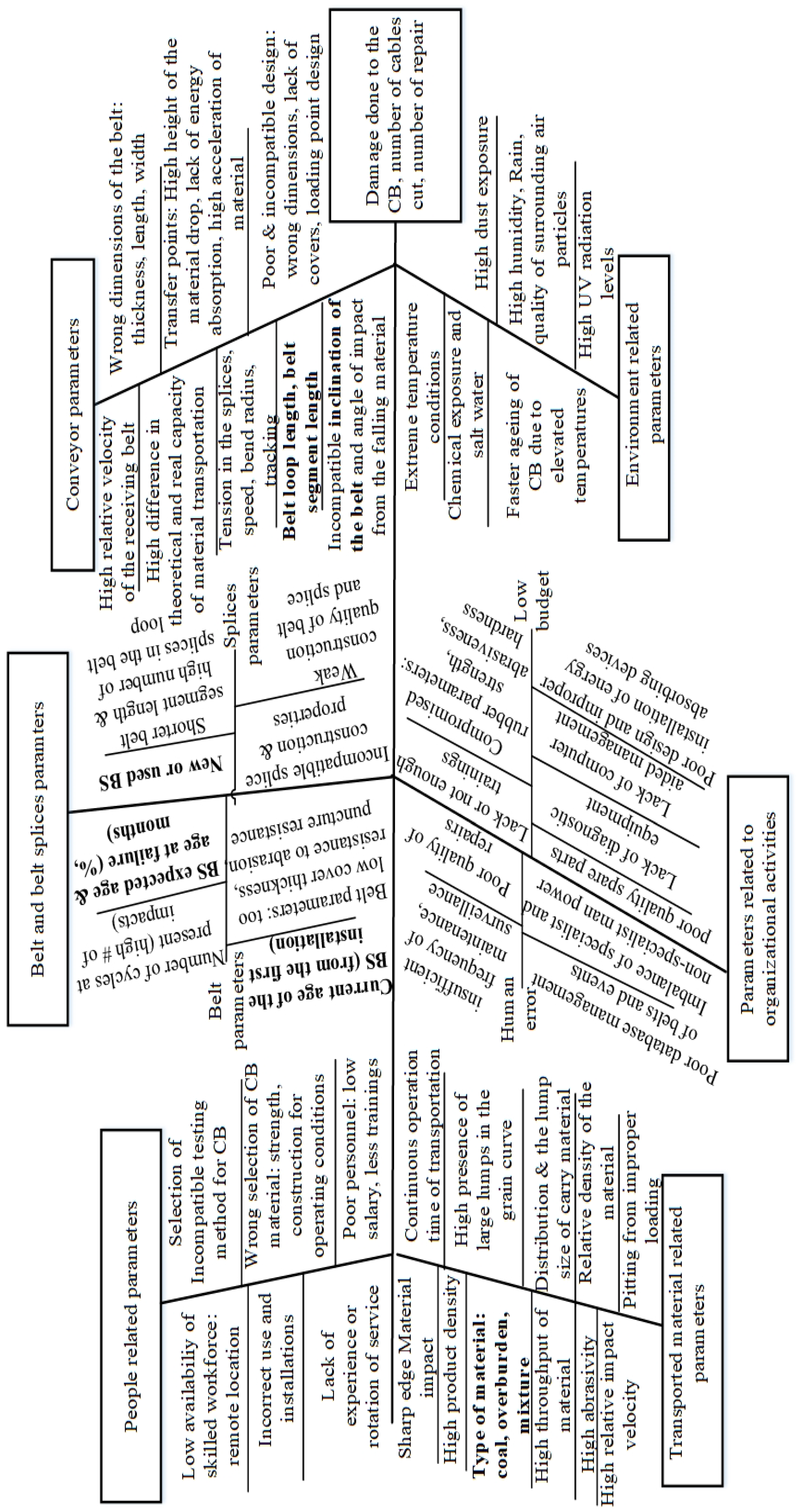
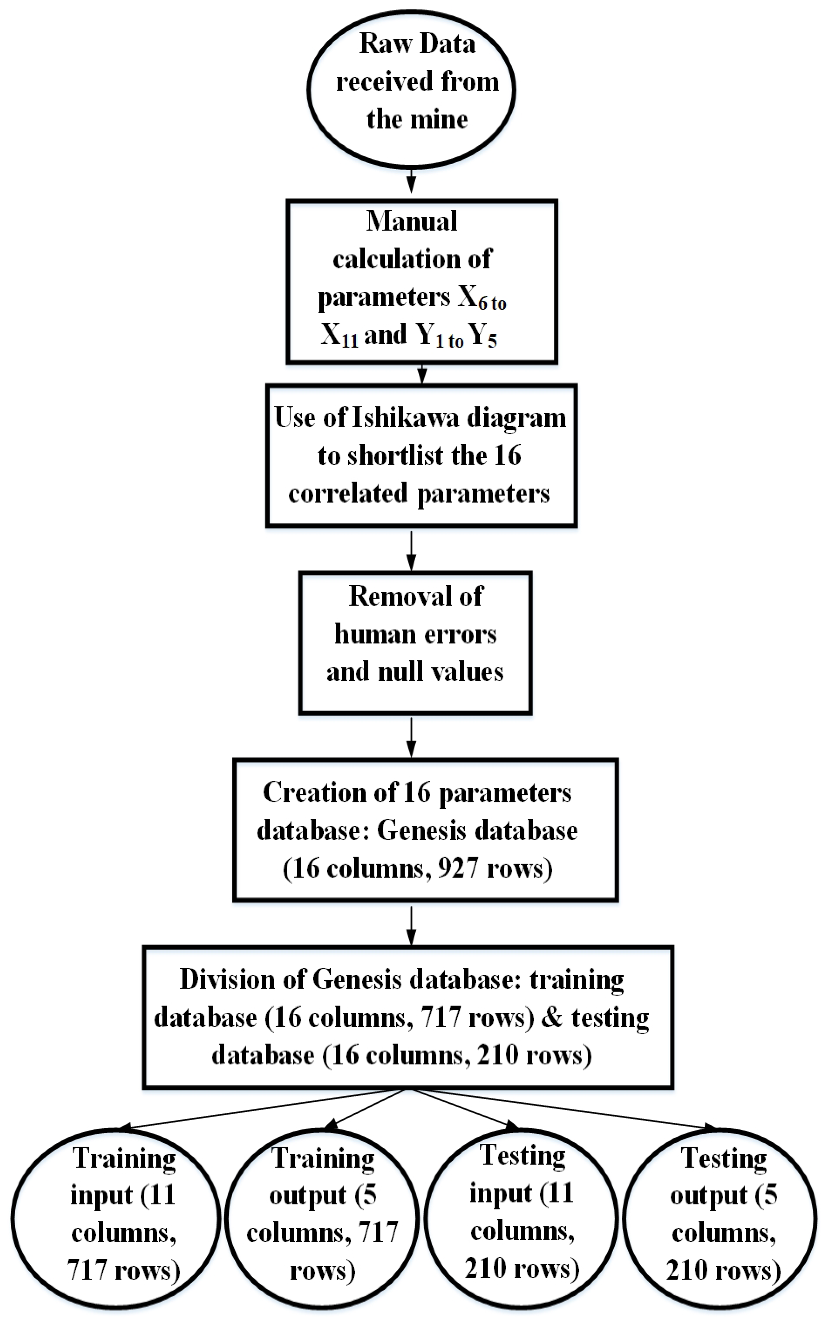
2.1. Datasets with Factors Influencing CB Damage and Operational Flowchart of the Study

The dataset, comprising 1112 rows in a spreadsheet detailing belt loops’ operating conditions, failures, and repairs, was obtained from the coal mine operated by PGE GiEK S.A., located in Belchatow, Poland. A total of 11 belt loops, incorporating 119 belt segments (BSs), were included in this study. Comprehensive information regarding belt segments, including purchase details, unique identification numbers (BS names), installation dates, splice activities during insertion, lengths, parameters, conveyor belt specifications, inclination, transported material, dismantling dates with reasons, and the fate of removed belt segments (disposed as waste or sent to the refurbishment plant), constituted the received data package. Data concerning failures (dates and locations) and repairs on conveyor belts (dates, dimensions, and locations) were sourced from routine visual monitoring by the maintenance crew, meticulously recorded in the repair and failure spreadsheet database.
The raw data provided insights into operational realities, particularly the impact of operating conditions on conveyor belt damage and service life. Variable selection for the study was guided by an Ishikawa diagram, as described in Figure 4. The Ishikawa diagram, developed through literature review, aided in identifying 16 correlated influential parameters (input variables: operating conditions) and influenced parameters (output variables: deterioration of the conveyor belt) from the quantitative databases received from the mine. The finalized dataset comprised the variables listed in Table 1 and Table 2.
The database encompassed parameters representing operating conditions, including parameters X 1 through X 5 . The degradation of the conveyor belt (CB) was documented in terms of the number of repairs and cable cuts, along with the age at each specific failure instance. Additional details, such as mounting dates, repair dates, and estimated damage areas to the rubber cover (determined via visual inspections), were also included in the databases obtained from the mine. Parameters X 6 through X 11 and Y 1 through Y 5 were manually computed based on individual instances of repairs or mounting. These instances were identified by repair dates or printing dates, indicating the mounting and removal of a belt segment on a specific belt loop. The manual calculations were conducted outside the mining facility, within the research group at the research institute presenting the current research findings.
After eliminating null values and human errors, the genesis database comprised 927 rows of records in a spreadsheet, with 16 columns representing parameters (11 for input parameters and 5 for output parameters). Subsequently, the genesis database was partitioned into a training database consisting of 717 rows (77.3% of the genesis database size) and a testing database comprising 210 rows (22.7% of the genesis database size). Both the training and testing databases were randomly sampled from the genesis database. Each training and testing database was further divided into two divisions: a database of input parameters ( X 1 to X 11 ) and a database of output parameters ( Y 1 to Y 5 ). This division resulted in four databases: two for training the neural network model (one containing input parameters and the other containing output parameters) and two for testing the trained neural network model (one for input parameters and the other for output parameters). The process of creating these four databases is illustrated in Figure 5. To investigate the impact of selected input parameters on output parameters, five distinct models were developed using five different combinations of output parameters with the same set of input parameters ( X 1 to X 11 ), as detailed in Table 3.
To further assess the performance of each of the five models (referred to as Model 1 to Model 5), three unique variations ( V 1 , V 2 , and V 3 ) of the training–testing datasets were generated. The division of records, totaling 11 belt loops (BLs) and 119 belt segments (BSs), was conducted as outlined in Table 4 and Table 5. Each variation of the training–testing datasets was created using different sets of belt segments. Consequently, in each variation ( V 1 , V 2 , and V 3 ), both the input and output database rows featured different combinations, owing to the division between the training and testing datasets derived solely from the genesis database.
This will contribute towards the investigation of the prediction performance of the models under different operating conditions and, thus, the trained model could be recognized as reliable way of predicting the deterioration of CB for future use at the mining site. The creation of three variations resulted in 15 different models, as illustrated in Table 6.
The flow chart of operations performed during this study is given in Figure 6, where we illustrate the collection of data through predictions of CBS failure and repair.
Step 1: Obtain the data files from the Belchatow coal mine, Poland. Identify and then rectify or remove the mistakes in the dataset (null values, typing errors, wrong records).
Steps 2 and 3: A total of 927 records were finalized after the execution of Step 1. Each training and prediction dataset was divided into the input (independent) and output (dependent) variables dataset.
Steps 4, 5, & 6: Choose the combination for the number of neurons and the number of layers in the hidden layers, the batch size based on the size of the training dataset, and the achieved training accuracy. Choose the limit for the number of epochs for training in order to avoid the issue of over-fitting (continuation of the training after achieving the maximum possible training accuracy) and under-fitting (stopping the training before the model reaches its maximum learning capacity) of the LSTM model.
Steps 7, 7.1, and 7.2: If the training accuracy with the chosen parameters for the neural network is not up to the expectations due to a lower or higher number of neurons, layers, batch size, and epochs, then their values have to be modified until the highest training accuracy results are achieved for the specific training dataset.
Steps 8, 9, and 10: Store the trained neural network model in the .h5 file format and then use the trained model to make predictions for the chosen values of the input variables dataset.
It is advisable to investigate the discrete pool of various operating conditions and properties of belt segments (BSs) within each belt loop (BL), as each mix of BSs in a BL necessitates specific optimal working conditions for the BL to operate as initially expected by the miners. These properties include:
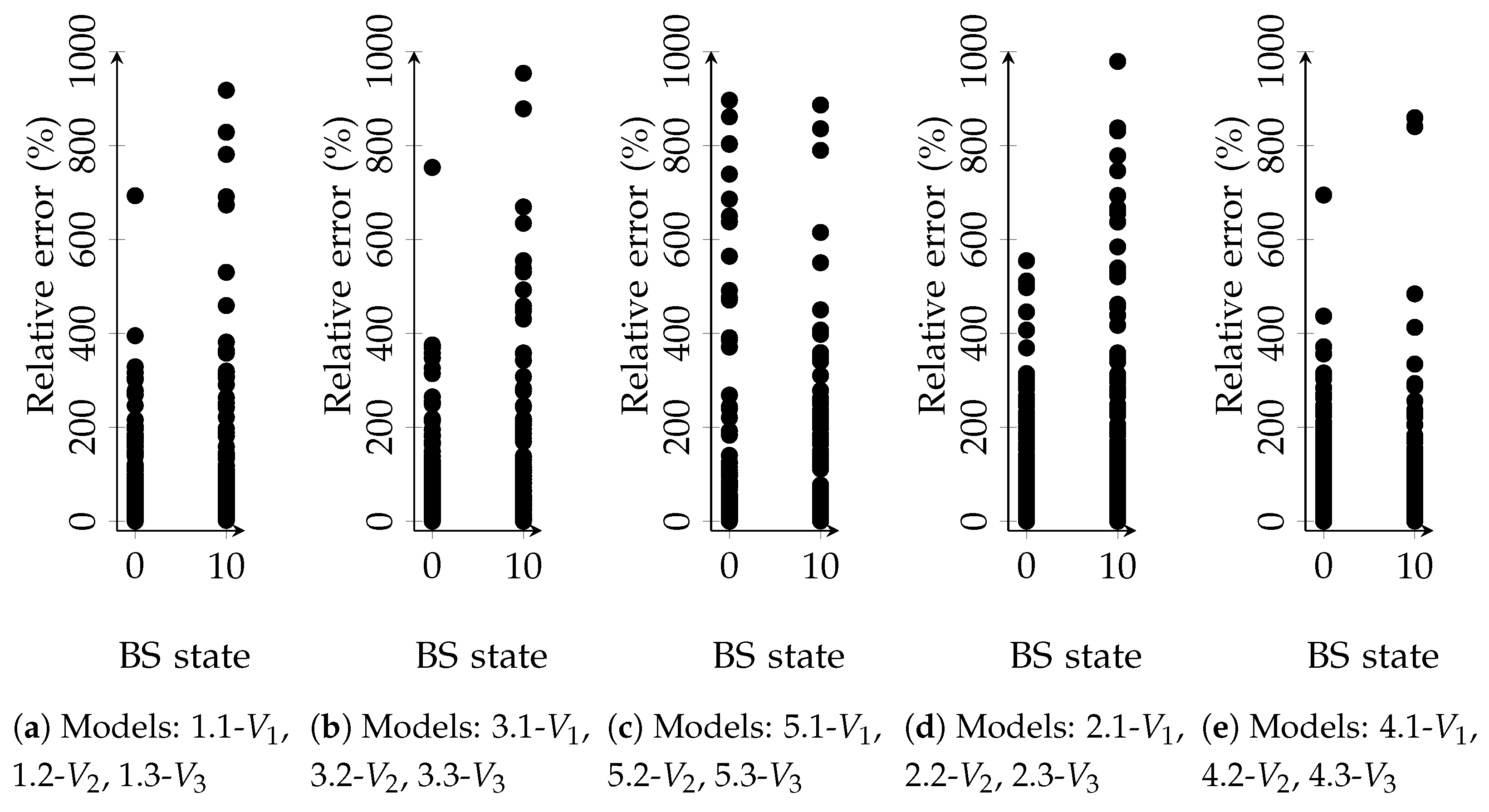
  • Whether the BS is new or moved.
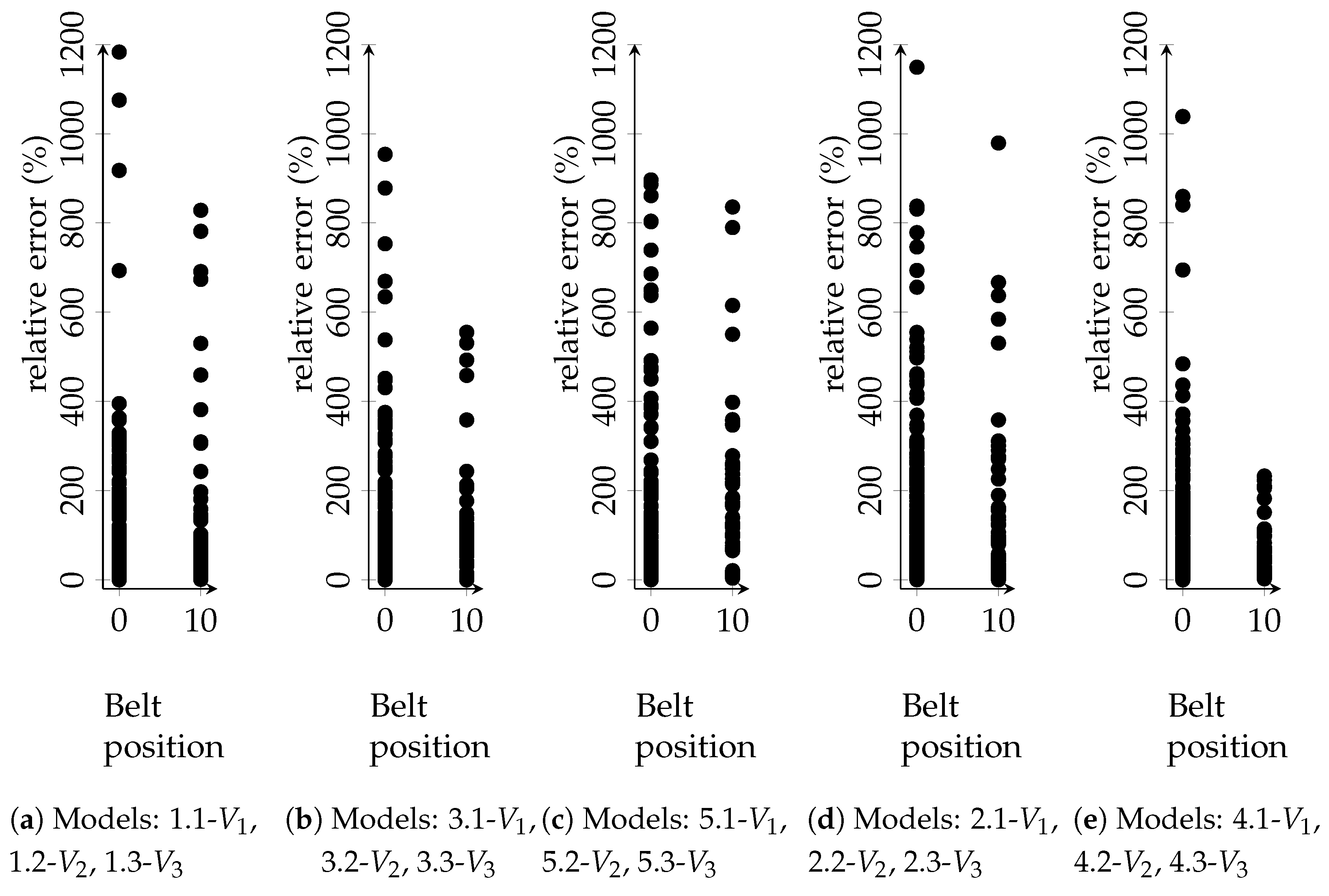
  • Belt position: whether it is flat or inclined.
  • Material being carried: coal, overburden, or a mixture of coal and overburden.
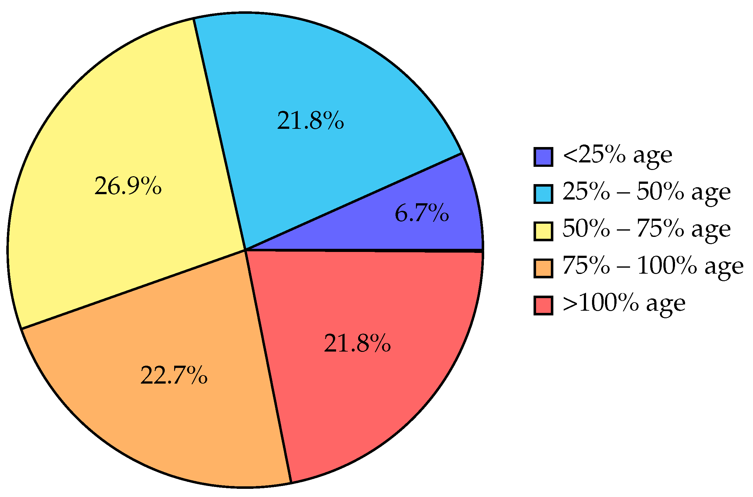
  • Age of the BS compared to its initial expectancy.
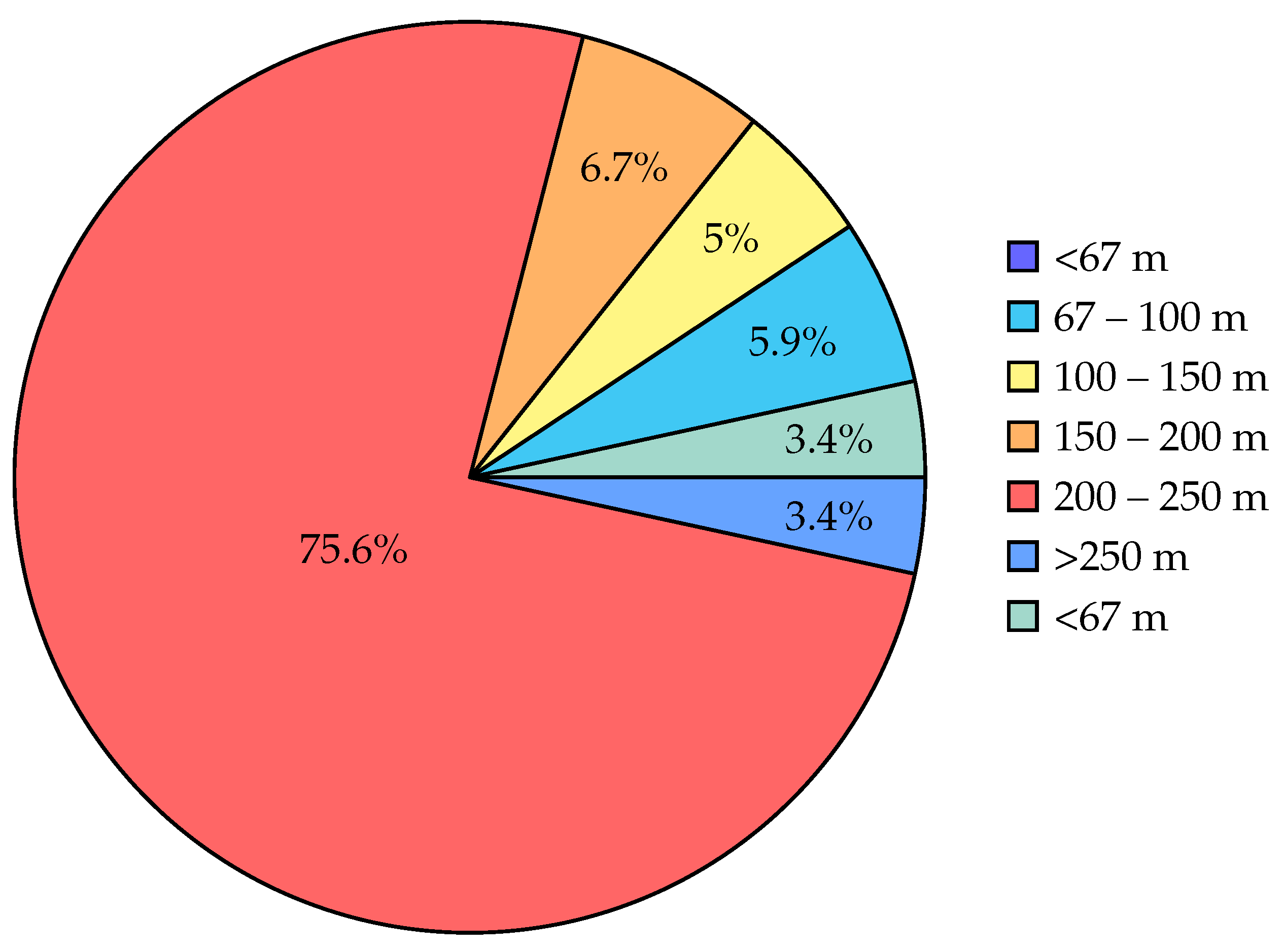
  • Total length of the BL and the total number of BSs within it.
As depicted in Figure 7, 75.6% of the records in the genesis database contained BSs with lengths ranging from 200 to 250 m. This is crucial for predictions, particularly for BSs with lengths less than 200 m. Shorter BSs are often older due to the removal of damaged belt fragments, which is less likely to occur when the belt is new.
Out of the total number of 119 BSs, 107 (90%) were used for the first time after purchase or moved from another BL, while 11 (9.2%) were refurbished once, and only 1 (0.8%) was refurbished twice. Notably, in the genesis database comprising 927 rows, BSs used for the first time (installed after purchase) accounted for 51.6% of the rows (478 rows), while moved BSs (new BSs that had been used on at least 2 conveyors, indicating a hidden history of damage) accounted for 48.4% of the rows (449 rows). When considering the number of BSs, 78 (65.5%) were previously used and moved from another BL, while 41 (34.5%) were new installations.
Coal represented only 13.4% of the data in the genesis database, while a mixture of coal, sand, and rock accounted for 62.2%, and overburden for 24.4%. If relative errors in predictions are lower for coal compared to other materials, it indicates that coal, as a carried material, exhibits uniformity in material handling during transportation and during the loading–unloading processes. Consequently, damage to the conveyor belt during material transportation becomes more predictable under specific operating conditions. On the other hand, predictions may encounter greater oddities with overburden and the mixture of coal-overburden due to the wide variety in rock and sand grain sizes and their sharpness/roughness compared to the relatively uniform qualities of coal, which is softer in comparison.
We consider another staggering fact, namely, that more than 85% of the records in the genesis database represent a flat belt inclination position and 14.3% inclined. The bias in the predictions for inclined belt loops ought to be specifically investigated. Inclined and flat conveyor loop positions have entirely different mechanism for the falling-carrying material and for the impact damage to the CB during material loading–unloading and transportation operations. Every BS has a life expectancy expected by operators (based on the average of past service lives) at the mine according to their experience and belt quality at the time of installation. The percentage of life completion for each BS at the time of dismantling from the loop as shown in Figure 8 is also decisive for the number of repairs and cable cuts, as older belts are more prone to critical damage, which leads to removal from the belt loop. Moreover, BL length and total number of BSs used in each BL to complete the loop, as shown in Figure 9, also constitute an important facet for any BL while investigating the operating conditions and their impact on the damage done to the BSs during operations. BLs having all BS lengths equivalent to one other indicates that BLs and BSs are newly in operation because, as the operational time continues, critically damaged small parts from the BSs are being removed and reintroduced after refurbishment. This working approach reduces the maintenance cost for the entire BS and also facilitates the repair work on a small damaged patch in a bigger BS.
The refined datasets served as the basis for training the artificial neural network (ANN). Databases comprising input and output parameters were utilized to develop ANN models aimed at understanding the deterioration of belt segments under specific operating conditions. During the training phase of the ANN model, it discerns hidden correlations between the input and output parameters of the system and stores this knowledge in the form of a hierarchical file format (.h5). Subsequently, the trained model was employed to forecast the behavior of the conveyor belt (CB) under potential future operating conditions and assess their impact on the output variables, including the service life of the belt and the associated number of repairs and cable cuts.

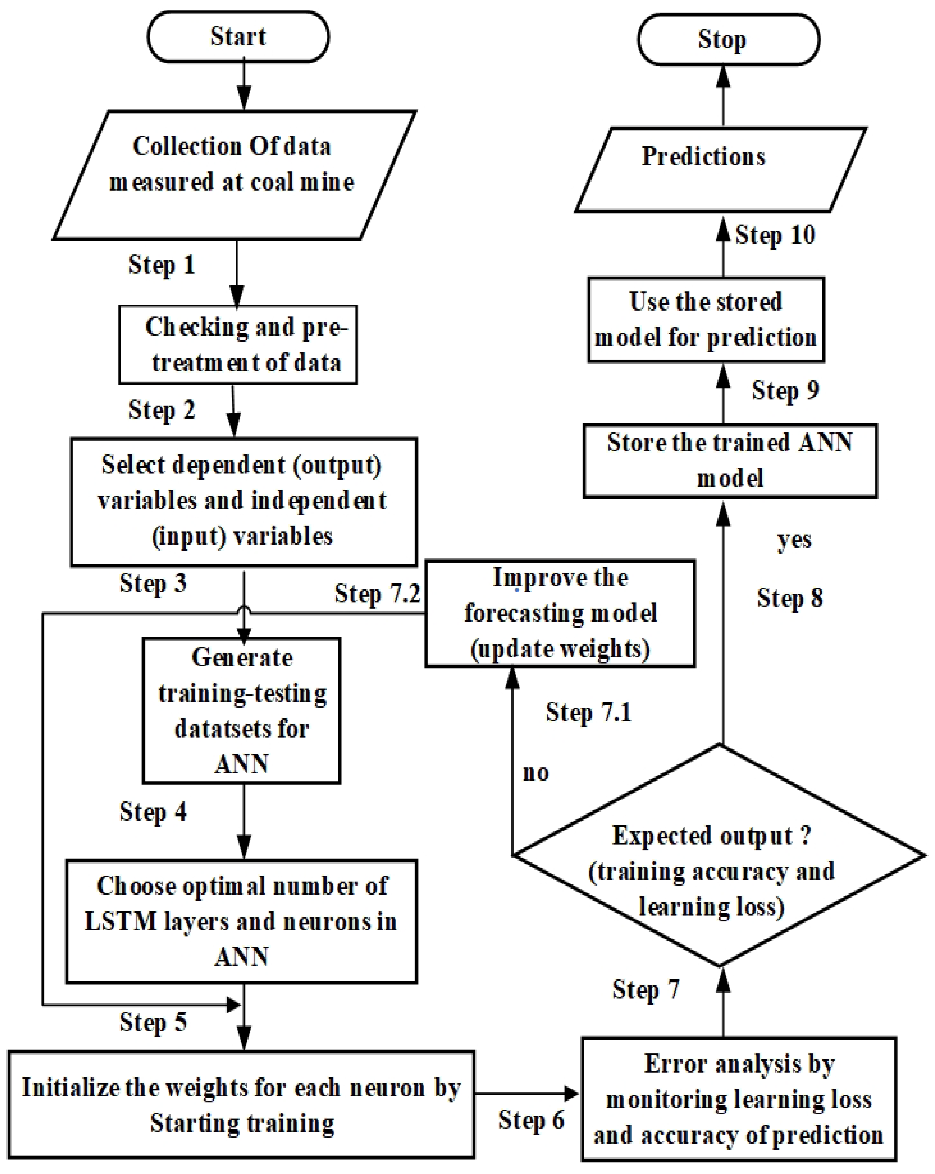
2.2. Artificial Neural Network

An artificial neural network (ANN) is a computational framework designed to emulate the information processing capabilities of the human brain. As a cornerstone of artificial intelligence and machine learning, ANNs are engineered to recognize patterns, make decisions, and predict outcomes based on input data. Below is a detailed description of its various components, functioning, and applications:
  • Structure of Artificial Neural Networks
    (a)
    Neurons (Nodes):
    • Neurons are the fundamental processing units of an ANN. Each neuron receives inputs, processes them, and generates an output.
    • A neuron combines the input data with a set of weights, adds a bias, and passes the result through an activation function to produce the final output.
    (b)
    Layers:
    • Input Layer: This is the first layer of the network, where the input data are fed into the system. Each node in this layer represents a distinct feature of the input data.
    • Hidden Layers: Situated between the input and output layers, these layers perform the main computations. Each hidden layer contains multiple neurons, and the network’s depth is determined by the number of hidden layers.
    • Output Layer: This is the layer that generates the final output of the network. The number of nodes in this layer corresponds to the number of desired output classes or values.
    (c)
    Weights and Biases:
    • Weights: Parameters within the network that transform input data within neurons. Each connection between neurons has an associated weight, determining the strength and direction of the input signal.
    • Biases: Values added to the weighted sum of inputs before passing through the activation function. Biases enable the activation function to shift left or right, which is crucial for learning complex patterns.
    (d)
    Activation Functions:
    • Activation functions determine whether a neuron should be activated, introducing non-linearity into the network and enabling it to learn more complex patterns.
    • Common activation functions include:
      Sigmoid: Produces outputs between 0 and 1, useful for probability-based outputs.
      Tanh (Hyperbolic Tangent): Outputs range from —1 to 1, centered around zero, making it beneficial for zero-centered data.
      ReLU (Rectified Linear Unit): Outputs the input directly if it is positive; otherwise, it outputs zero. It helps mitigate the vanishing gradient problem.
  • How ANNs Work
    (a)
    Forward Propagation:
    • This involves passing the input data through the network to obtain the output.
    • In each layer, a neuron computes a weighted sum of its inputs, adds a bias, and applies an activation function to generate an output.
    • This process continues from the input layer, through the hidden layers, to the output layer, where the final prediction or classification is generated.
    (b)
    Learning (Training):
    • Training an ANN involves adjusting its weights and biases to minimize the error between its predictions and the actual target values.
    • A common approach to training involves supervised learning, where the network is trained on a labeled dataset. Each example in the dataset consists of an input and its corresponding correct output.
    (c)
    Back-propagation:
    • Back-propagation is a fundamental algorithm for training ANNs. It functions by propagating the error backward from the output layer to the input layer, adjusting the weights and biases to minimize the error.
    • The process involves:
      Calculating the error at the output layer.
      Using the derivative of the activation function to determine the gradient of the error with respect to each weight.
      Adjusting the weights and biases in the direction that reduces the error, typically using an optimization algorithm like gradient descent.
  • Types of Neural Networks
    (a)
    Feedforward Neural Networks:
    • The simplest type of ANN where connections between nodes do not form cycles.
    • Information moves in one direction—from input nodes, through hidden nodes (if any), to output nodes.
    (b)
    Convolutional Neural Networks (CNNs):
    • Primarily used for image and video recognition.
    • They use convolutional layers to automatically and adaptively learn spatial hierarchies of features from input images.
    (c)
    Recurrent Neural Networks (RNNs):
    • Designed to recognize sequences and patterns in sequential data.
    • They have connections that form directed cycles, allowing information to persist across steps.
    (d)
    Generative Adversarial Networks (GANs):
    • Consist of two neural networks, a generator and a discriminator, that compete against each other.
    • Used for generating new, synthetic instances of data that can pass for real data.
Artificial neural networks (ANNs) are powerful computational tools modeled after the neural structure of the human brain. Comprising interconnected neurons organized into layers, ANNs adjust the weights of these connections during training to minimize prediction errors. They are widely applied in fields such as image and speech recognition, natural language processing, and autonomous vehicles. Despite their successes, ANNs present challenges related to data requirements, computational demands, and interpretability. As research and technology progress, ANNs continue to evolve, providing increasingly sophisticated and efficient solutions for complex problems.

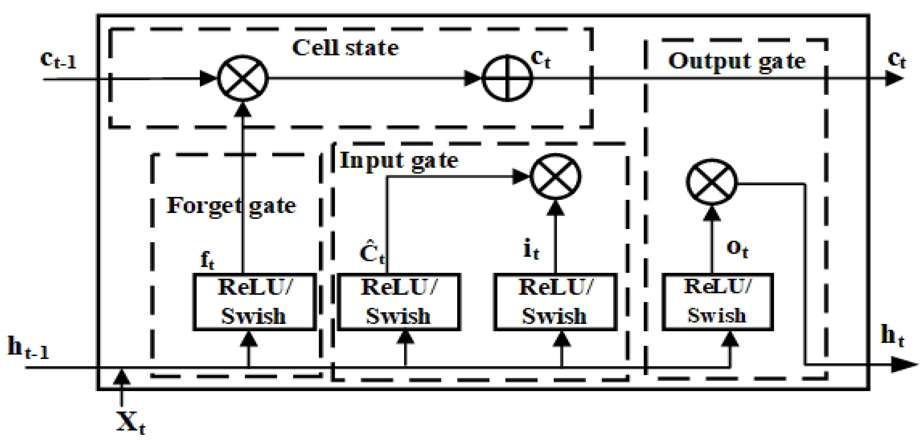
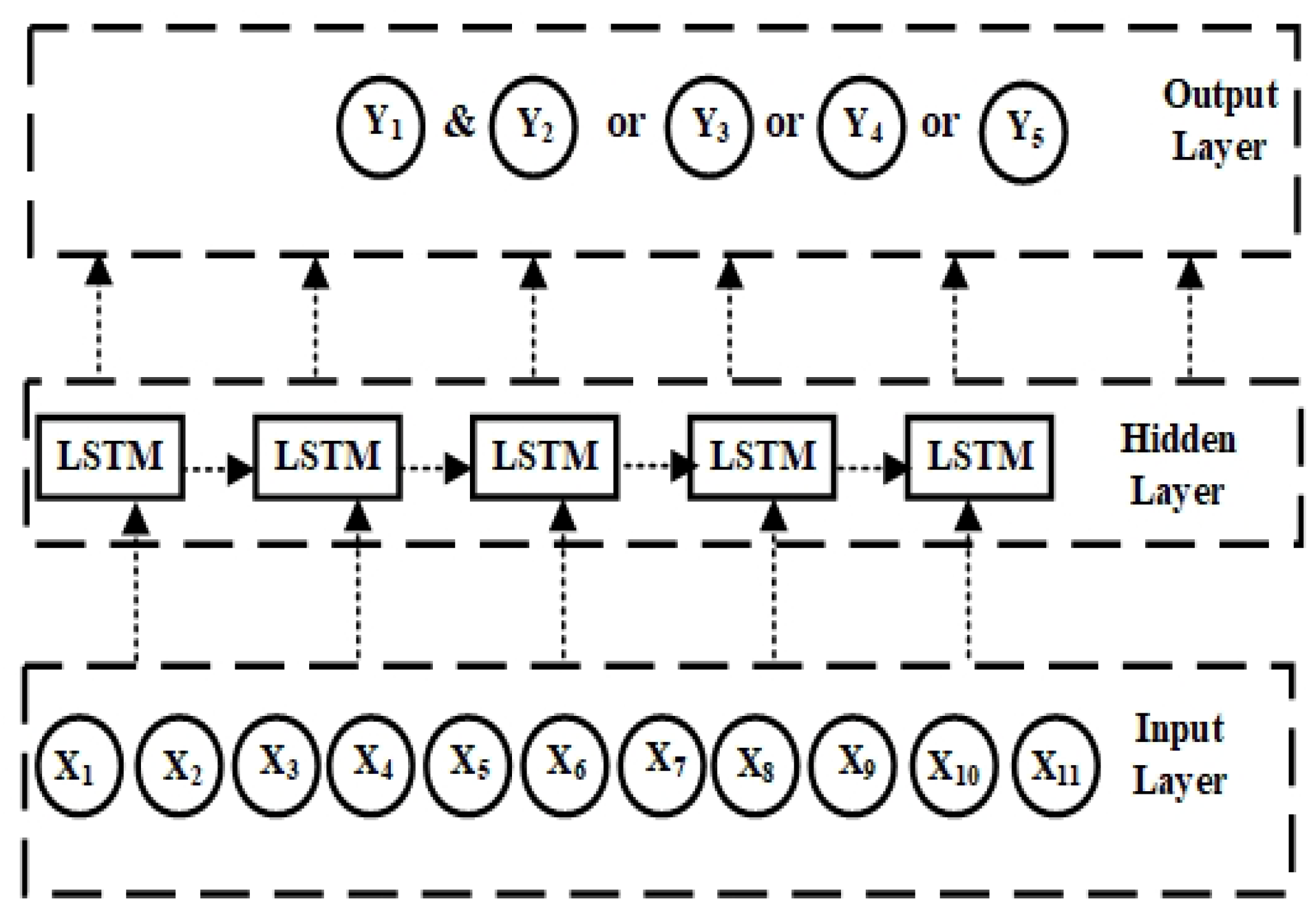
2.3. Long Short-Term Memory (LSTM) Model

The LSTM model, a type of recurrent neural network (RNN), was introduced by Hochreiter and Schmidhuber [50,51]. While RNNs enable multivariate time series prediction, they struggle to learn long-term dependencies among variables due to the vanishing gradient problem [52]. This limitation is addressed in the LSTM model through the incorporation of three gates: the input gate, output gate, and the forget gate, as illustrated in Figure 10. These memory units enable the LSTM network to forget outdated information and incorporate new information. The effectiveness of updating old and new memories depends on the chosen time delay (in this study, a time delay of 1 (repair and cable cut instance) was selected) of the data used for training the LSTM neural network. For example, in a time series consisting of five time steps ( t 1 to t 5 ), if the chosen time delay is three time steps, the information in the LSTM network progresses as follows: ( t 1 , t 2 , t 3 ) ( t 2 , t 3 , t 4 ) ( t 3 , t 4 , t 5 ) . The LSTM model was implemented using the Google Colab platform, with the Python programming language utilized for code execution. Python libraries such as TensorFlow, NumPy, Keras, pandas, Matplotlib, and scikit-learn were employed for programming tasks.
Referring to the architecture of the LSTM shown in Figure 10, t = time step, c t = cell state information, f t = forget gate at t, i t = input gate at t, c t 1 = previous time step, C ^ t = value generated by the tanh function, h t = hidden state, h t 1 = previous hidden state, o t = output gate state, and X t = input at the particular time.
During the study, different numbers of hidden layers and neurons were explored and compared. Combination 2, as listed in Table 7, was selected for the neural network parameters, as it yielded the highest validation accuracy during the training of the LSTM network (with the highest achievable accuracy being 100). The mean squared error (MSE) loss function, where the value of MSE decreases with increasing training accuracy, was employed. Various batch sizes (2, 4, 8, and 16) were tested for each model, with a batch size of 16 ultimately chosen, as other tested batch sizes did not significantly impact the training accuracy.
A range of optimizers, including Adam, Nadam, Adamax, RMSprop, and stochastic gradient descent (SGD), were employed along with back-propagation to update the weights within the neural network. Additionally, six different activation functions—ReLU, Swish, sigmoid, tanh, Leaky ReLU, and softmax—were experimented with. Based on achieved training accuracy and learning loss during the training of the neural network across different instances, the optimizers Adam, Nadam, and RMSprop, along with the activation functions ReLU and Swish, were finalized due to their comparatively superior results.
The ReLU activation function employed in this study offers several advantages: (1) computational simplicity, as the rectifier function is straightforward to implement compared to tanh and sigmoid activation functions, which require exponential calculations; (2) representational sparsity, as it outputs true zero values for negative inputs, allowing hidden layers in neural networks to contain one or more true zero values; (3) linear behavior, making it easier to optimize the neural network when its behavior is linear or close to linear, thereby avoiding vanishing gradients; and (4) suitability for training deep neural networks. Additionally, the Swish activation function facilitates data normalization, leading to faster convergence and learning of the neural network. It is also suitable for deep neural networks and facilitates small gradient updates during training, which is essential for efficient back-propagation in deep networks.
Referring to the present study, the flow of data during training of the LSTM network is shown in Figure 11, where a total of 11 input variables were introduced to IL, one or two variables were assigned to the OL, and inter-dependencies between IL and OL variables were established in HL.

3. Results and Discussion

The discussion of the varying record shares of different operating conditions and belt segment (BS) properties/conditions in the genesis database was presented in Section 2.1. Now, referring to Table 8 and Table 9, the distribution between the three versions of training and testing variations ( V 1 , V 2 , and V 3 ) with different combinations of BSs for training and testing is explained. The shares presented in Table 8 and Table 9 can serve to justify the specific behavior of the models during predictions. Observing the variations V 1 , V 2 , and V 3 , it is evident that different numbers of used BSs were employed. This depiction can be utilized to establish a correlation between the share of specific categories in the genesis database and their representation in variations V 1 , V 2 , and V 3 . Such analysis can lead to the conclusion that the trained models are applicable for future operating conditions that are not confined to any specific range of operating conditions or BS conditions.
The following indicators were used to evaluate the performance of different models mentioned in Table 10, Table 11, Table 12, Table 13 and Table 14:
A: Percent of 210 prediction instances having a relative error < 50% compared to mine records.
B: Percent of 210 prediction instances having a relative error between 50–100% compared to mine records.
C: Percent of 210 prediction instances having a relative error > 100% compared to the records.
Green color: models with comparatively best prediction results based on indicators and median value.
Table 10 and Table 11 illustrate that, for both Models 1 and 2, variation V 2 exhibited comparatively superior values for indicator A. However, in the case of Model 2, the prediction results for variations V 1 and V 3 indicated a significant deterioration in indicator A values. Notably, BL2 and BL3 were not included in the testing database for variation V 2 . It is conceivable that BL2 and BL3 experienced significant issues as noted by the mine operator(s) during specific instances, potentially impacting the recorded number of repairs.
Furthermore, as detailed in Table 4 and Table 5, version V 2 comprised the highest number of BSs for training and the comparatively lowest number of BSs for testing.
In contrast to the results observed for Models 1 and 2 as depicted in Table 10 and Table 11, the results for Model 3, presented in Table 12, indicate that variation V 3 exhibits comparatively better values for indicator A than variations V 1 and V 2 . Furthermore, the results for Model 4, outlined in Table 13, reveal that variation V 2 has the lowest value (2.8% for cumulative number of cable cuts) for indicator C. However, the values for indicator A are the highest for variation V 1 .
All variations— V 1 , V 2 , and V 3 —exhibit indicator A values of more than 55% for Model 5, as shown in Table 14, indicating that the generated Model 5 can be utilized for all future operating conditions, rendering it reliable. Furthermore, Table 14 also illustrates that employing only one variable as an output improves predictions compared to models where two variables need to be correlated to the set of inputs.
In summary, considering the gap between the highest and lowest values for indicator A within the prediction results for Models 1 to 5, as detailed in Table 10, Table 11, Table 12, Table 13 and Table 14, it becomes evident that no specific variation of the testing–training dataset (from V 1 , V 2 , or V 3 ) consistently outperforms or underperforms others. Hence, the best-performing models highlighted in green in Table 10, Table 11, Table 12, Table 13 and Table 14 can be employed for specific targeted variables to assess the performance of the conveyor belt in future operating conditions.
Figure 12, Figure 13, Figure 14, Figure 15 and Figure 16 depict the results for all models mentioned in Table 10, Table 11, Table 12, Table 13 and Table 14, indicating that trends were predicted in the majority of cases, while seasonalities were also analogous to records from the mine for most of the belt segments. Instances numbered from 0 to 210 represent comparisons for variation V 1 , whereas instances 211 to 420 represent comparisons for variation V 1 , and instances 421 to 630 account for comparisons for variation V 3 .
Belt segments (BSs) moved from another belt loop (BL) have high relative errors in predictions across all models, as shown in Figure 17. All repaired and reintroduced BSs (which are then counted as new BSs) have already completed a certain portion of their expected service life at the time of installation. This implies that these BSs have hidden histories of repair and damage, which were not conveyed to the AI model. Therefore, high relative errors for this specific category are expected, making it difficult for the AI model to estimate the total number of repairs and cable cuts accurately. Consequently, estimating the age of new BSs is also challenging. Furthermore, there is no standard rule for dismantling a specific BS from the BL, as this decision is mostly based on human judgment, experience, and the current availability of resources for maintenance and replacement.
As mentioned in the earlier sections, another factor responsible for the high relative error and outstanding number of errors could be the disproportionate record share in the genesis database. Specifically, we note the following: (i) 90% of BSs (107 BSs by number) belong to the first use after purchase or BSs moved from another BL, while only 10% of BSs (12 BSs by number) are refurbished; (ii) in the genesis database, 65.5% of BSs (78 BSs) belonged to moved BSs (moved from another BL), whereas 34.5% of BSs (41 BSs) were new; and (iii) 478 rows (51.6% of the total 927 rows) in the genesis database accounted for new BS data, while 449 rows (48.4% of the total 927 rows) accounted for moved BS data.
Regarding carry material, a mixture of coal and overburden on the conveyor belt (CB) accounted for the highest numbers in relative error prediction, as shown in Figure 18. Coal had the lowest numbers for relative error, whereas overburden was second in terms of relative error numbers. This suggests that coal poses uniformity in material handling during transportation. In contrast, a mixture of coal and overburden consists of varying proportions between coal and overburden, with the grain size and wear capacity of overburden also differing chronologically. Hence, it is evident that relative errors are high for this specific category.
Relative errors in predictions for belt positions (flat or inclined) are shown in Figure 19. All illustrated models demonstrate similarities, with the total number of prediction points having relative errors higher than 100% being greater for flat belts. A noteworthy concurrent fact is that the inclined belt record share in the genesis database is less than 15%. The angle of impact plays a decisive role during material transportation, contributing to the damage done to the conveyor belt (CB) due to the impact of the carry material. Simultaneously, despite the significant gap in the percentage record share for both categories, inclined belt segments recorded lower relative error numbers for all models. The possible reason could be that inclined conveyor positions minimize the uncertainty regarding the angle of impact, leading to more uniform damage patterns from material handling processes.
Belt loop (BL) length showed relative errors according to postulations, as shown in Figure 20. A few individual instances exhibited the highest relative errors in predictions for BLs having lengths greater than 2.4 Km. However, considering the overall total number of instances with relative errors higher than 100%, these were more frequent for BLs with lengths less than 2.4 km. Specifically, Model 5, where age is modeled, showed high relative error numbers for BL lengths less than 1.2 km. This behavior is attributed to the fact that all three versions ( V 1 , V 2 , and V 3 ) of testing and training datasets had 75% of the records for ages less than 60 months. BLs with short ages and short loop lengths imply frequent changes of the BS during operation, as they have to repeat more cycles compared to longer BLs. This indicates that the main influences (number of repairs and cable cuts) deciding the service life of the belt (modeled in Model 5) accounted for high relative errors during training, which is reflected in the prediction results. This is due to human decision-making regarding recording specific damages and shifting the BS for repairs based solely on visual inspection at regular intervals.
Furthermore, CB3, CB7, CB8, and CB10 were the BLs with lengths less than 1045 m. CB10 and CB8 had outstanding numbers for relative errors in predictions. BS67 in CB8 and BS88 in CB10 are new BSs in their respective belt loops. This indicates that BSs with no past failure history data are more susceptible to higher relative error numbers in predictions. The main reason could be human intervention, which decides the removal of a specific BS from a specific BL, involving human expertise and experience only, without any standard rule defining a certain threshold for removing BSs from the loop. Furthermore, cyclical visual inspections at regular intervals are conducted at mine facilities, and minor damages to the CB are mostly ignored unless the damage becomes significant enough to be included in the next batch of repairs and maintenance. Moreover, BS88 comprises one-third of the total length of the CB10 belt loop, thus offering more area for material carry, which increases the potential for damage compared to shorter BSs.
The length of the belt segments (BSs) also played a decisive role in the relative errors, as shown in Figure 21. BSs with lengths greater than 225 m exhibited the highest number of relative errors overall. Notably, the percentage record share mentioned in Table 8 and Table 9 indicates that all versions of the testing and training datasets had more than 75% of the total records for BSs longer than 200 m. Damaged patches from the BS are removed from the healthy parts of the BS, which reduces the total length of the BS. Additionally, a BS length greater than 200 m suggests that the BS is new and indicates that the damaged BS patch may not been removed from the parent BS for repairs and maintenance even once. The decision to remove the BSs from a belt loop (BL) is entirely up to the mining operators, as mentioned earlier. The lower number of relative errors for shorter BSs indicates that the models were better able to estimate the number of repairs and the number of cable cuts, closely aligning with the records from the mine, compared to predictions for longer BSs. This suggests that longer damaged areas involve more uncertainties for the models.
Therefore, it can be concluded that a more thorough approach to recording failures is needed, and relying solely on human visual inspection is not sufficient.

4. Conclusions

This research models conveyor belt (CB) damage using machine learning, focusing on the number of repairs and cable cuts during service life under specific operating conditions. Key parameters for neural network optimization (e.g., optimizers, activation functions, batch size, number of epochs) are identified, and the significance of data collection techniques in capturing failure and repair events at a coal mine is highlighted. Traditional regression models are hindered by multi-collinearity, human errors, and limited reliability in data. They suffer from issues like small sample sizes, data point eccentricities, and overfitting. AI models, however, can retrain with new datasets, reestablishing input–output relationships within neural network weights.
Data from the Belchatow coal mine (1112 rows initially, 927 post-preprocessing) were used to train and test an LSTM neural network, with a training–testing split of 77.3% and 22.7%, respectively. Five different output variables (number of repairs and cable cuts, cumulative repairs and cuts, instantaneous age) were correlated with 11 input parameters (belt length and inclination, BS conditions, previous BS history, completed percentage service life, transported material). Models (1 to 5) were tested with various optimizers (RMSprop, Adam, Adamax, Nadam, and SGD) and activation functions (ReLU, Swish, sigmoid, tanh, Leaky ReLU, and softmax) with different batch sizes (2, 4, 8, and 16) and epochs (15 to 150). Adam, Nadam, and RMSprop optimizers as well as ReLU and Swish activation functions showed superior performance with 60 epochs and a batch size of 16. Model reliability was established by training and testing on three dataset variations ( V 1 , V 2 , and V 3 ), with performance evaluated using three indicators (A, B, and C). Indicators accounted for different ranges of the percentage of the total of 210 prediction instances having relative error compared to mine records (A: <50%, B: >50% and <100%, and C: >100%). Selected models had high indicator A values and low indicator C values, with median relative error predictions ranging from 26% to 55%.
Moved BSs exhibited high relative errors due to unknown histories affecting prediction accuracy. Flat belt positions had higher relative errors due to a disproportionate record share between flat (85.7%) and inclined (14.3%) conveyors. Diverse datasets on different angles of impact could improve correlation mapping. Coal as a material had the lowest relative error, while coal and sand–rock mixtures had the highest due to uncertain proportions and large lumps. Short belt loops (<2.4 km) had high relative errors, likely due to frequent BS changes and increased loading cycles. BSs with lengths greater than 225 m experienced stochastic failures, leading to high prediction errors. No dataset variant ( V 1 , V 2 , or V 3 ) consistently outperformed others across all models.
Current data collection, based on visual inspections, is insufficient due to subjective decision-making and recording only significant visible failures. Smaller undetected failures are often ignored, impacting the condition assessment of conveyor belt segments. AI application is limited by these insufficient data. While AI can predict failure events based on historical data, comprehensive predictions require more reliable data. Implementing diagnostic devices like magnetic or X-ray scanners for detailed core damage detection can enhance database reliability and AI prediction accuracy. Future work involves integrating data from the DiagBelt+ steel cord diagnostic system in the Belchatow mine for improved model performance [32,53,54,55,56].

Author Contributions

Conceptualization, P.P., L.J., A.R. and A.B.; methodology, P.P. and A.R.; software, P.P.; validation, A.R., A.B. and L.J.; formal analysis, P.P., L.J. and A.R.; investigation, P.P., L.J. and A.R.; resources, L.J. and A.R.; data curation, P.P., L.J. and A.R.; writing—original draft preparation, P.P.; writing—review and editing, P.P., L.J. and A.B.; visualization, P.P., L.J., A.R. and A.B.; supervision, L.J. and A.B.; project administration, L.J. and A.B.; funding acquisition, A.B. All authors have read and agreed to the published version of the manuscript.

Funding

This research received no external funding.

Data Availability Statement

The datasets presented in this article are not readily available because authors do not have permission from the mine operators to share them publicly.

Conflicts of Interest

The authors declare no conflicts of interest.

Abbreviations

The following abbreviations are used in this manuscript:
AIArtificial intelligence
ANNArtificial neural network
BLBelt loop
BSBelt segment
CBConveyor belt
CBSConveyor belt system
c t 1 Previous time step
C ^ t Value generated by the tanh function
c t Cell state information
f t Forget gate at t
h t Hidden state
h t 1 Previous hidden state
HLHidden layer
i t Input gate at t
ILInput layer
KmKilometer
LSTMLong short-term memory
mmeters
MSEMean squared error
OLOutput layer
o t Output gate state
ReLURectified linear unit
RNNRecurrent neural network
SGDStochastic gradient descent
tTime step
V 1 Variation 1
V 2 Variation 2
V 3 Variation 3
X t Input at the particular time

References

  1. Koivisto, K. Conveyor Engineering; BoD-Books on Demand: Helsinki, Finland, 2018. [Google Scholar]
  2. Skocir, T. Mechanical Conveyors: Selection and Operation; Routledge: London, UK, 2018. [Google Scholar]
  3. Song, X.; Yu, X.; Zhou, C.; Xu, B.; Chen, L.; Yagoub, A.E.A.; Emeka, O.C.; Wahia, H. Conveyor belt catalytic infrared as a novel apparatus for blanching processing applied to sweet potatoes in the industrial scale. LWT 2021, 149, 111827. [Google Scholar] [CrossRef]
  4. Thapa, K.N.K.; Kalaivani, S.; Vanaja, S.; Sheela, J.J.J.; Deepika, Y. Differential Amplifier Based Speed Monitoring Circuit for Airport and Production Industry. In Proceedings of the 2021 Fifth International Conference on I-SMAC (IoT in Social, Mobile, Analytics and Cloud)(I-SMAC), Palladam, India, 11–13 November 2021; pp. 1–4. [Google Scholar]
  5. Wijaya, E.O.; Setyadi, A.; Rimawan, E. Minimize Conveyor Belt Damage in Coal-Fired Power Plants Using SEM-PLS and FMEA Methods. Nveo-Nat. Volatiles Essent. Oils J. NVEO 2021, 8, 1283–1289. [Google Scholar]
  6. Rosita, N.D. Coal Transport Through The Conveyor Belt: Literature Study Of Process And Supporting Factors. J. Sains Teknol. Transp. Marit. 2023, 5, 44–49. [Google Scholar] [CrossRef]
  7. Kold, J.; Silverman, C. Conveyors used in the food industry. In Handbook of Hygiene Control in the Food Industry; Elsevier: Amsterdam, The Netherlands, 2016; pp. 367–382. [Google Scholar]
  8. Chen, J.; Lau, S.K.; Chen, L.; Wang, S.; Subbiah, J. Modeling radio frequency heating of food moving on a conveyor belt. Food Bioprod. Process. 2017, 102, 307–319. [Google Scholar] [CrossRef]
  9. Rashid, S.; Bashir, O.; Majid, I. Different mechanical conveyors in food processing. In Transporting Operations of Food Materials within Food Factories; Elsevier: Amsterdam, The Netherlands, 2023; pp. 253–263. [Google Scholar]
  10. Kumar, N. Fundamentals of conveyors. In Transporting Operations of Food Materials within Food Factories; Elsevier: Amsterdam, The Netherlands, 2023; pp. 221–251. [Google Scholar]
  11. Żur, T.; Hardygóra, M. Belt Conveyors in Mining; Śląsk Publishers: Katowice, Poland, 1979. [Google Scholar]
  12. Jurdziak, L.; Blazej, R.; Bajda, M. Conveyor Belt 4.0. In Intelligent Systems in Production Engineering and Maintenance; Springer: Cham, Switzerland, 2019; pp. 645–654. [Google Scholar]
  13. Rao, D.S. The Belt Conveyor: A Concise Basic Course; CRC Press: Boca Raton, FL, USA, 2020. [Google Scholar]
  14. Zrnić, N.; Đorđević, M.; Gašić, V. Historical background and evolution of belt conveyors. Found. Sci. 2022, 29, 225–255. [Google Scholar] [CrossRef]
  15. Zrnić, N.; Đorđević, M.; Gašić, V. History of belt conveyors until the end of the 19th century. In International Symposium on History of Machines and Mechanisms; Springer: Cham, Switzerland, 2022; pp. 210–223. [Google Scholar]
  16. Solomon, M.D.; Heineken, W.; Scheffler, M.; Birth, T. Energy Conveyor Belt—A Detailed Analysis of a New Type of Hydrokinetic Device. Energies 2023, 16, 2188. [Google Scholar] [CrossRef]
  17. Chen, X.; Kong, Y.; Wang, M.; Huang, X.; Huang, Y.; Lv, Y.; Li, G. Wear and aging behavior of vulcanized natural rubber nanocomposites under high-speed and high-load sliding wear conditions. Wear 2022, 498–499, 204341. [Google Scholar] [CrossRef]
  18. Andrejiova, M.; Grincova, A.; Marasova, D. Measurement and simulation of impact wear damage to industrial conveyor belts. Wear 2016, 368–369, 400–407. [Google Scholar] [CrossRef]
  19. Nins, B.; Penagos, J.J.; Moreira, L.; Münch, D.; Falqueto, P.; Viáfara, C.C.; da Costa, A.R. Abrasiveness of iron ores: Analysis of service-worn conveyor belts and laboratory Dry Sand/Rubber Wheel tests. Wear 2022, 506, 204439. [Google Scholar] [CrossRef]
  20. Andrejiova, M.; Grincova, A. Classification of impact damage on a rubber-textile conveyor belt using Naïve-Bayes methodology. Wear 2018, 414, 59–67. [Google Scholar] [CrossRef]
  21. Marasova, D.; Andrejiova, M.; Grincova, A. Dynamic Model of Impact Energy Absorption by a Conveyor Belt in Interaction with the Support System. Energies 2022, 15, 64. [Google Scholar] [CrossRef]
  22. Hrabovsky, L.; Fries, J. Transport Performance of a Steeply Situated Belt Conveyor. Energies 2021, 14, 7984. [Google Scholar] [CrossRef]
  23. Doroszuk, B.; Krol, R.; Wajs, J. Simple Design Solution for Harsh Operating Conditions: Redesign of Conveyor Transfer Station with Reverse Engineering and DEM Simulations. Energies 2021, 14, 4008. [Google Scholar] [CrossRef]
  24. Bindzár, P. Impact cradle–the most critical place regarding to failure of conveyors belt. In Proceedings of the Development of New Technologies and Equipment for Mine Haulage and Hoisting, 5th International Symposium on Mine Haulage and Hoisting, Beograd–Vrdnik, Belgrade, Serbia, 25–27 September 2002; Volume 25, p. 27. [Google Scholar]
  25. Marasová, D. Mathematical and Experimental Support for Belt Conveyors. In Ostrava: Vysoká Škola Báňská—Technická Univerzita Ostrava, Czech Republic 76 s. : il.; 2013. Available online: https://katalog.vsb.cz/records/4f0ad9dc-312e-487c-b3c6-ec743f33d980 (accessed on 19 January 2023).
  26. Gharahasanlou, A.N.; Mokhtarei, A.; Khodayarei, A.; Ataei, M. Fault tree analysis of failure cause of crushing plant and mixing bed hall at Khoy cement factory in Iran. Case Stud. Eng. Fail. Anal. 2014, 2, 33–38. [Google Scholar] [CrossRef] [PubMed]
  27. Cao, J.; Huang, H.; Jiao, R.; Pei, J.; Xu, Y.; Wang, Y. The study of wear particle emissions of soft rubber on rolling contact under braking conditions. Wear 2022, 506, 204431. [Google Scholar] [CrossRef]
  28. Kirjanów-Błażej, A.; Jurdziak, L.; Błażej, R.; Rzeszowska, A. Calibration procedure for ultrasonic sensors for precise thickness measurement. Measurement 2023, 214, 112744. [Google Scholar] [CrossRef]
  29. Fedorko, G.; Molnar, V.; Marasova, D.; Grincova, A.; Dovica, M.; Zivcak, J.; Toth, T.; Husakova, N. Failure analysis of belt conveyor damage caused by the falling material. Part I: Experimental measurements and regression models. Eng. Fail. Anal. 2014, 36, 30–38. [Google Scholar] [CrossRef]
  30. Cerny, J.; Kyas, K.; Krumal, M.; Manas, D.; Manas, M.; Stanek, M. WEAR PROCESS OF TIRES. In Annals of DAAAM & Proceedings; DAAAM International: Vienna, Austria, 2010; pp. 1189–1190. [Google Scholar]
  31. Szrek, J.; Jakubiak, J.; Zimroz, R. A Mobile Robot-Based System for Automatic Inspection of Belt Conveyors in Mining Industry. Energies 2022, 15, 327. [Google Scholar] [CrossRef]
  32. Bajda, M.; Błażej, R.; Jurdziak, L. Analysis of changes in the length of belt sections and the number of splices in the belt loops on conveyors in an underground mine. Eng. Fail. Anal. 2019, 101, 436–446. [Google Scholar] [CrossRef]
  33. Bajda, M.; Błażej, R.; Jurdziak, L.; Hardygóra, M. Impact of differences in durability of vulcanized and adhesive joints on the operating costs of conveyor belts in underground mines. In Zeszyty Naukowe Instytutu Gospodarki Surowcami Mineralnymi Polskiej Akademii Nauk; Instytut Gospodarki Surowcami Mineralnymi i Energią PAN: Krakow, Poland, 2017; pp. 71–88. [Google Scholar]
  34. Wozniak, D.; Hardygóra, M. Aspects of Selecting Appropriate Conveyor Belt Strength. Energies 2021, 14, 6018. [Google Scholar] [CrossRef]
  35. Jurdziak, L.; Bajda, M.; Blazej, R. Estimation of Purchase and Replacement Costs of Conveyor Belts and their Splices in an Underground Mine Based on their Durability. Iop Conf. Ser. Earth Environ. Sci. 2019, 221, 012099. [Google Scholar] [CrossRef]
  36. Bugaric, U.; Tanasijevic, M.; Polovina, D.; Ignjatovic, D.; Jovancic, P. Lost production costs of the overburden excavation system caused by rubber belt failure; [Koszty utraconej produkcji wywołane uszkodzeniem gumowej taśmy transportowej w układzie maszynowym do zdejmowania nadkładu]. Eksploat. Niezawodn. 2012, 14, 333–341. [Google Scholar]
  37. Ilic, D. Development of design criteria for reducing wear in iron ore transfer chutes. Wear 2019, 434-435, 202986. [Google Scholar] [CrossRef]
  38. Maintenance of Belt Conveyor Systems in Poland—An Overview. Available online: https://www.wipro.com/natural-resources/predictive-failure-model-for-conveyor-belt-systems/ (accessed on 19 January 2023).
  39. Bajda, M.; Hardygóra, M.; Marasová, D. Energy Efficiency of Conveyor Belts in Raw Materials Industry. Energies 2022, 15, 3080. [Google Scholar] [CrossRef]
  40. Kawalec, W.; Król, R. Generating of electric energy by a declined overburden conveyor in a continuous surface mine. Energies 2021, 14, 4030. [Google Scholar] [CrossRef]
  41. Blazej, R.; Jurdziak, L. Condition-based conveyor belt replacement strategy in lignite mines with random belt deterioration. IOP Conf. Ser. Earth Environ. Sci. 2017, 95, 042051. [Google Scholar] [CrossRef]
  42. van der Laan, B.Z. System reliability analysis of belt conveyor. In Transportation Engineering; Delft University of Technology: Delft, The Netherlands, 2016. [Google Scholar]
  43. Fedorko, G.; Molnár, V.; Michalik, P.; Dovica, M.; Kelemenová, T.; Tóth, T. Failure analysis of conveyor belt samples under tensile load. J. Ind. Text. 2019, 48, 1364–1383. [Google Scholar] [CrossRef]
  44. Zimroz, R.; Król, R. Failure analysis of belt conveyor systems for condition monitoring purposes. Min. Sci. 2009, 128, 255. [Google Scholar]
  45. Bajda, M.; Hardygóra, M. Laboratory tests of operational durability and energy-efficiency of conveyor belts. IOP Conf. Ser. Earth Environ. Sci. 2019, 261, 012002. [Google Scholar] [CrossRef]
  46. Zimroz, R.; Hardygóra, M.; Blazej, R. Maintenance of Belt Conveyor Systems in Poland—An Overview. In Proceedings of the 12th International Symposium Continuous Surface Mining-Aachen 2014; Springer International Publishing: Cham, Switzerland, 2015; pp. 21–30. [Google Scholar]
  47. Belchatów Mine, Poland. Available online: https://euracoal.eu/info/country-profiles/poland (accessed on 19 January 2023).
  48. Jurdziak, L.; Błażej, R.; Burduk, A.; Bajda, M.; Kirjanów-Błażej, A.; Kozłowski, T.; Olchówka, D. Optimization of the operating costs of conveyor belts in a mine in various strategies of their replacement and diagnostics. Transp. Przem. Masz. Rob. 2020, 4, 50. [Google Scholar]
  49. Parmar, P.; Burduk, A.; Jurdziak, L. Ishikawa Diagram Indicating Potential Causes for Damage Occurring to the Rubber Conveyor Belt Operating at Coal Mining Site. In Proceedings of the International Conference on Intelligent Systems in Production Engineering and Maintenance, Wrocław, Poland, 13–15 September 2023; Springer: Berlin/Heidelberg, Germany, 2023; pp. 704–713. [Google Scholar]
  50. Hochreiter, S.; Schmidhuber, J. Long Short-Term Memory. Neural Comput. 1997, 9, 1735–1780. [Google Scholar] [CrossRef] [PubMed]
  51. Medsker, L.; Jain, L.C. Recurrent Neural Networks: Design and Applications; CRC Press: Boca Raton, FL, USA, 1999. [Google Scholar]
  52. Hochreiter, S. The Vanishing Gradient Problem During Learning Recurrent Neural Nets and Problem Solutions. Int. J. Uncertain. Fuzziness-Knowl.-Based Syst. 1998, 06, 107–116. [Google Scholar] [CrossRef]
  53. Olchówka, D.; Blażej, R.; Jurdziak, L. Selection of measurement parameters using the DiagBelt magnetic system on the test conveyor. J. Phys. Conf. Ser. 2022, 2198, 012042. [Google Scholar] [CrossRef]
  54. Kirjanów-Błażej, A.; Jurdziak, L.; Burduk, R.; Błażej, R. Forecast of the remaining lifetime of steel cord conveyor belts based on regression methods in damage analysis identified by subsequent DiagBelt scans. Eng. Fail. Anal. 2019, 100, 119–126. [Google Scholar] [CrossRef]
  55. Błażej, R.; Jurdziak, L.; Kozłowski, T.; Kirjanów, A. The use of magnetic sensors in monitoring the condition of the core in steel cord conveyor belts–Tests of the measuring probe and the design of the DiagBelt system. Measurement 2018, 123, 48–53. [Google Scholar] [CrossRef]
  56. Rzeszowska, A.; Jurdziak, L.; Błażej, R.; Kirjanów-Błażej, A. Application of Clustering and SOM Analysis for Identification of Conveyor Belt Damage Based on Data from the Diagbelt + Magnetic System. In Advances in Production; Springer: Cham, Switzerland, 2023; pp. 461–475. [Google Scholar]
Figure 1. Schematic diagram of conveyor belt.
Energies 17 03497 g001
Figure 2. Damaged conveyor.
Energies 17 03497 g002
Figure 3. Damaged patch in conveyor belt.
Energies 17 03497 g003
Figure 4. Ishikawa diagram listing parameters affecting conveyor belt damage at the coal mine [49].
Energies 17 03497 g004
Figure 5. Flow chart: testing and training database creation.
Energies 17 03497 g005
Figure 6. Flow chart of operations followed in the presented study.
Energies 17 03497 g006
Figure 7. Belt segment length comparison in the genesis database.
Energies 17 03497 g007
Figure 8. Percent share in the genesis database for age at present compared to expected age by miners at the time of installation.
Energies 17 03497 g008
Figure 9. BL length and total BSs in each BL.
Energies 17 03497 g009
Figure 10. Architecture of a long short-term memory (LSTM) recurrent neural network (RNN).
Energies 17 03497 g010
Figure 11. An example of data flow in the LSTM network.
Energies 17 03497 g011
Figure 12. Predicted number of repairs vs. repairs recorded at mine (models: 1.1— V 1 , 1.2— V 2 , 1.3— V 3 ).
Energies 17 03497 g012
Figure 13. Predicted numbers of cable cuts vs. cable cuts recorded at mine (models: 3.1- V 1 , 3.2- V 2 , 3.3- V 3 ).
Energies 17 03497 g013
Figure 14. Predicted age vs. age recorded at mine at specific instance of standstill (models: 5.1- V 1 , 5.2- V 2 , 5.3- V 3 ).
Energies 17 03497 g014
Figure 15. Predicted number of cumulative repairs vs. cumulative repair numbers calculated from mine data (models: 2.1- V 1 , 2.2- V 2 , 2.3- V 3 ).
Energies 17 03497 g015
Figure 16. Predicted number of cumulative cable cuts vs. cumulative number of cable cuts calculated from mine data (models: 4.1- V 1 , 4.2- V 2 , 4.3- V 3 ).
Energies 17 03497 g016
Figure 17. Belt segment (BS) state’s (new: 0, moved from another BL: 10) impact on predictions for different models.
Energies 17 03497 g017
Figure 18. Transported materials’ (0: coal, 5: mixture of coal, rock, and sand, 10: overburden) impact on predictions for different models.
Energies 17 03497 g018
Figure 19. Conveyor positions’ (0: flat, 10: inclined) impact on predictions made by different models.
Energies 17 03497 g019
Figure 20. Belt loop (BL) length’s impact on predictions made by different models.
Energies 17 03497 g020
Figure 21. Belt segment (BS) length’s impact on predictions made by different models.
Energies 17 03497 g021
Table 1. List of dependent variables.
Y 1 Age at current
srepair: standstill
Y 2 Number of small repairs
at current standstill
Y 3 Cumulative number of small
repairs at current standstill
ine Y 4 Number of cable/s cut
at current standstill
Y 5 Cumulative number of
cuts at current standstill
Table 2. List of independent variables.
X 1 Belt loop length
X 2 Belt segment length
X 3 Transported material
X 4 Inclination of the
conveyor belt
X 5 New or moved
belt segment
X 6 Completed percentage life
compared to human estimation
ine X 7 Age at previous
repair: standstill
X 8 Number of small repairs
during previous standstill
ine X 9 Previous cumulative
number of small repairs
ine X 10 Previous number
of cables cut
X 11 Previous cumulative
number of cuts
Table 3. Five main models designed in the present study.
ModelInput ParametersOutput Parameters
Model 1 X 1 to X 11 Y 1 and Y 2
Model 2 X 1 to X 11 Y 1 and Y 3
Model 3 X 1 to X 11 Y 1 and Y 4
Model 4 X 1 to X 11 Y 1 and Y 5
Model 5 X 1 to X 11 Y 1
Table 4. Total number of belt loop (BL) and belt segment (BS) distribution in genesis database and in different testing databases.
V 1 Database V 2 Database V 3 Database
BL & BS used for training11 & 9211 & 9811 & 79
BL & BS used for testing11 & 279 & 2111 & 40
Table 5. Number of belt loop (BL) and belt segment (BS) distribution in genesis database and in different testing databases.
Genesis Database V 1 Database for Testing V 2 Database for Testing V 3 Database for Testing
BL1: BS1 to BS8BL1: BS1, BS8BL1: BS2BL1: BS3 to BS7
BL2: BS9 to BS13BL2: BS9 to BS11 BL2: BS12, BS13
BL3: BS14 to BS16BL3: BS16 BL3: BS14, BS15
BL4: BS17 to BS33BL4: BS27 to BS29, BS32, BS33BL4: BS17BL4: BS19 to BS26, BS28
BL5: BS35 to BS47BL5: BS47BL5: BS46BL5: BS34 to BS42, BS43
BL6: BS48 to BS59BL6: BS57BL6: BS48BL6: BS50 to BS56
BL7: BS60 to BS64BL7: BS62BL7: BS63, BS64BL7: BS60, BS61
BL8: BS65 to BS74BL8: BS71 to BS73BL8: BS65, BS66BL8: BS67, BS68
BL9: BS75 to BS83BL9: BS81to BS83BL9: BS75, BS80BL9: BS77 to BS78
BL10: BS84 to BS92BL10: BS84 to BS86 BS92BL10: BS87BL10: BS88
BL11: BS93 to BS119BL11: BS102, BS103, BS112, BS115, BS116BL11: BS93 to BS101, BS119BL11: BS107, BS109, BS111, BS113, BS114, BS117,
Table 6. All models designed in the present study.
ModelInput ParametersOutput Parameters
Model 1.1- V 1 X 1 to X 11 Y 1 and Y 2
Model 1.2- V 2 X 1 to X 11 Y 1 and Y 2
Model 1.3- V 3 X 1 to X 11 Y 1 and Y 2
Model 2.1- V 1 X 1 to X 11 Y 1 and Y 3
Model 2.2- V 2 X 1 to X 11 Y 1 and Y 3
Model 2.3- V 3 X 1 to X 11 Y 1 and Y 3
Model 3.1- V 1 X 1 to X 11 Y 1 and Y 4
Model 3.2- V 2 X 1 to X 11 Y 1 and Y 4
Model 3.3- V 3 X 1 to X 11 Y 1 and Y 4
Model 4.1- V 1 X 1 to X 11 Y 1 and Y 5
Model 4.2- V 2 X 1 to X 11 Y 1 and Y 5
Model 4.3- V 3 X 1 to X 11 Y 1 and Y 5
Model 5.1- V 1 X 1 to X 11 Y 1
Model 5.2- V 2 X 1 to X 11 Y 1
Model 5.3- V 3 X 1 to X 11 Y 1
Table 7. Selection of neuron and layer combinations.
Combi-nationInput Layer (IL) NeuronsNeurons × Hidden Layer (HL)Output Layer (OL) NeuronsBatch SizeEpochsAccuracy % for Training/
Validation
111 36 × 4 2166097/75
211 36 × 3 2166097/83
311 36 × 7 2166098/71
411 36 × 3 2169098/77
Table 8. Share of the different parameters’ status condition in different testing datasets.
Parameters’ Status Condition V 1 V 2 V 3 |Maximum —  Minimum|
≤200 m BS length24.8%15.2%10.9%13.9%
>200 m BS length75.2%84.8%89.1%13.9%
Transported
material: coal
10.9%9.6%8.5%2.4%
Transported material:
mixture of coal and sand, rock
51.9%49.5%52.8%3.3%
Transported material:
overburden
37.2%40.9%38.7%3.7%
Belt position: flat84.2%86.2%84.8%2%
Belt position: inclined15.8%13.8%15.2%2%
Belt condition: new47.2%84.8%62.4%37.6%
Belt condition:
moved from another BL
52.8%15.2%37.6%37.6%
Age at current
repair 60 months
77.6%87.1%79%9.5%
Age at previous repair > 60 months22.4%12.9%21%9.5%
Table 9. Share of the different parameters’ status condition in different training datasets.
Parameters’ Status Condition V 1 V 2 V 3 |Maximum —  Minimum|
≤200 m BS length10.3%13.2%14.4%4.1%
>200 m BS length89.7%86.8%85.6%4.1%
Transported
material: coal
6.8%7.3%7.5%0.7%
Transported material:
mixture of coal and sand, rock
52.8%53.6%52.6%1%
Transported material:
overburden
40.4%39.1%39.9%1.3%
Belt position: flat85.6%85.0%85.6%0.6%
Belt position: inclined14.4%15%14.4%0.6%
Belt condition: new52.8%41.9%48.4%10.9%
Belt condition:
moved from another BL
47.2%58.1%51.6%10.9%
Age at current
repair 60 months
82.5%79.6%82%2.9%
Age at previous repair > 60 months17.5%20.4%18%2.9%
Table 10. Prediction results (in %) for Model 1, indicating share for indicators A, B, and C.
ParametersActivation FunctionTesting Dataset VersionOptimizerMedian Value of Relative ErrorABC
AgeReLU V 1 Nadam60471140
Repairs45533411
AgeReLU V 2 Nadam2765925
Repairs2971217
AgeReLU V 3 Nadam47511830
Repairs46501931
Table 11. Prediction results (in %) for Model 2, indicating share for indicators A, B, and C.
ParametersActivation FunctionTesting Dataset VersionOptimizerMedian Value of Relative ErrorABC
AgeSwish V 1 Adam40531531
Cumulative repairs111242351
AgeSwish V 2 Adam33621521
Cumulative repairs3180153
AgeSwish V 3 Adam55481734
Cumulative repairs131221957
Table 12. Prediction results (in %) for Model 3, indicating share for indicators A, B, and C.
ParametersActivation FunctionTesting Dataset VersionOptimizerMedian Value of Relative ErrorABC
AgeSwish V 1 Adam49502919
Cable cuts52462626
AgeSwish V 2 Adam28591129
Cable cuts56492822
AgeSwish V 3 Adam36621422
Cable cuts34621621
Table 13. Prediction results (in %) for Model 4, indicating share for indicators A, B, and C.
ParametersActivation FunctionTesting Dataset VersionOptimizerMedian Value of Relative ErrorABC
AgeReLU V 1 RMSprop26709.520
Cumulative number
of cable cuts
55433125
AgeReLU V 2 RMSprop33581228
Cumulative number
of cable cuts
5243542.8
AgeReLU V 3 RMSprop42541827
Cumulative number
of cable cuts
107232255
Table 14. Prediction results (in %) for Model 5, indicating share for indicators A, B, and C.
Activation FunctionTesting Dataset VersionOptimizerMedian Value of Relative ErrorABC
ReLU V 1 Nadam36651221
ReLU V 2 Nadam27581624
ReLU V 3 Nadam22666.228.2
Disclaimer/Publisher’s Note: The statements, opinions and data contained in all publications are solely those of the individual author(s) and contributor(s) and not of MDPI and/or the editor(s). MDPI and/or the editor(s) disclaim responsibility for any injury to people or property resulting from any ideas, methods, instructions or products referred to in the content.

