Systematic Design of Cathode Air Supply Systems for PEM Fuel Cells

Abstract

To increase system efficiency and power density, the cathode air path of Polymer Electrolyte Membrane Fuel Cells (PEM FCs) is supercharged using electrically driven air bearing centrifugal compressors. To maximize system efficiency, the cathode air supply system must be designed to optimally fulfill the requirements of the PEM FC system while obeying the design constraints imposed by the electric compressor drive and the air bearing system. This article proposes a dedicated design process for PEM FC cathode air compressors. Using physically based component models, the impact of varying cathode stoichiometry and operating pressure on PEM FC system performance is assessed to derive the system efficiency optimal compressor operating strategy. The centrifugal compressor stage is subsequently designed to achieve optimum efficiency on this operating line using meanline performance models and three-dimensional computational fluid dynamics simulations. Novel test procedures and measurement equipment are employed to validate the compressor design. The design process is demonstrated using a PEM FC passenger car application as an example. It is shown that significant performance and efficiency gains are achievable when tailoring the cathode air supply system to the application at hand. In the given example, effective compressor efficiency is increased by Δη_eff = 12%. Along with an optimized compressor operating strategy, an overall PEM FC system efficiency gain of Δη_sys = 2.7% is achieved.

1. Introduction

Mobile powertrains based on polymer electrolyte membrane fuel cells (PEM FCs) offer the potential of high energy and power density as well as short refueling times. This makes the PEM FC technology particularly suited for the transportation sector [1].

Currently, great efforts are made to increase the system efficiency and power density of PEM FC systems. The cathode air path is supercharged to increase oxygen partial pressure. Reaction losses are reduced and maximum current density is increased, consequently improving stack efficiency and power density [2].

Electrically driven centrifugal compressors are predominantly used for supercharging, as they offer unmatched efficiency and power density for the flow and pressure ratio requirements at hand [3]. The cathode air supply system must be optimally matched to the overall PEM FC system to achieve maximum system efficiency. For exhaust gas turbochargers of internal combustion engines, this matching process is state-of-the-art [4,5]: The interaction between the internal combustion engine and exhaust gas turbocharger is well understood and can be simulated with a high degree of accuracy [6,7]. The turbomachine geometry optimization process has been proven over multiple generations of successive design iterations for various engine types [8,9,10].

For PEM FC systems, this maturity level is not achieved yet, requiring a more profound design approach [2]. Oftentimes, the exact compressor performance targets are unknown and must be derived using system simulation and analysis. The electric compressor drive and air bearing system (required for oil-free operation) impose additional design constraints compared to exhaust gas turbochargers [11]: The electric machine exhibits a trade-off between rated speed and rated power impacting impeller sizing [12]. The air bearing system limits the allowable impeller thrust load [13]. Accordingly, established design tools and workflows cannot be used directly [14].

In this article, a novel design process for PEM FC cathode air supply systems based on electrically driven centrifugal compressors is introduced.

Physically based component models for the PEM FC stack and the membrane humidifier are utilized to understand the influence of cathode air mass flow rate (stoichiometry) and operating pressure on PEM FC system performance (cf. Section 2.1 and Section 2.2). The component models are integrated into a model of the PEM FC powertrain to derive the cathode air compressor operating strategy yielding maximum system efficiency (optimum operating line, cf. Section 2.3).

The design constraints imposed by the electric machine and the air bearing system are discussed and a preliminary compressor design process is derived to yield a suitable centrifugal compressor geometry for the PEM FC application at hand (cf. Section 4). Centrifugal compressor operating behavior is assessed using meanline performance models and three-dimensional computational fluid dynamics simulations. Optimization techniques are subsequently used to maximize compressor efficiency on the optimum operating line (cf. Section 5).

Finally, reliable test procedures and associated measurement equipment are developed to validate the cathode air compressor design and to refine the performance models and simulations, where necessary (cf. Section 6).

Due to small expected production numbers, development budgets for PEM FC systems will be limited in the foreseeable future. This yields the requirement for a streamlined, highly automated and generalized design workflow. The approach proposed in the following shall not only allow the designer to find the optimum cathode air compressor for a given PEM FC system. It shall also foster the profound communication between OEM system designers and component suppliers by allowing both sides to clearly define boundary conditions and performance targets in a quantitative manner. This way, unnecessary design iterations are eliminated, and development time and associated costs are significantly reduced.

2. Fuel Cell System Simulation

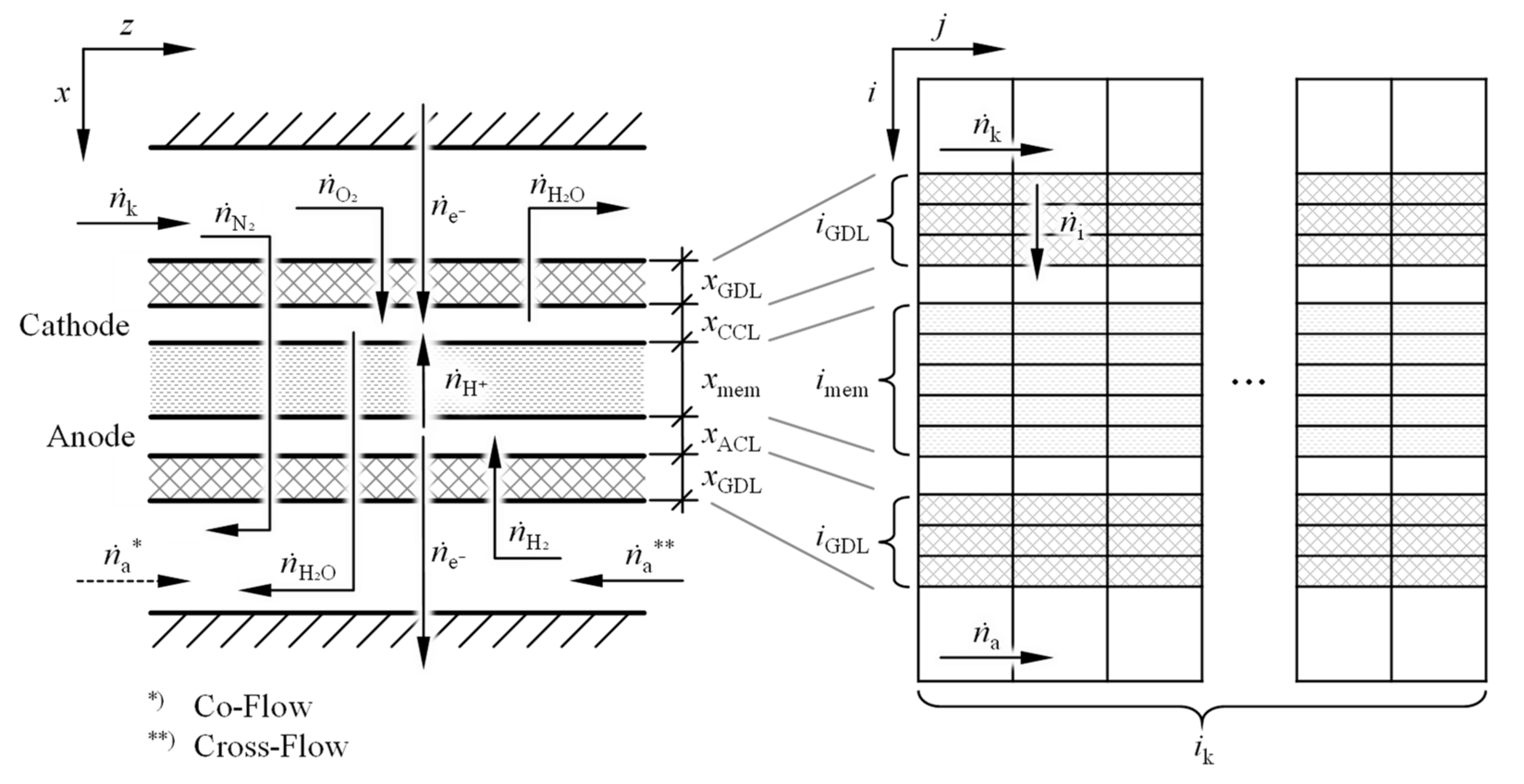
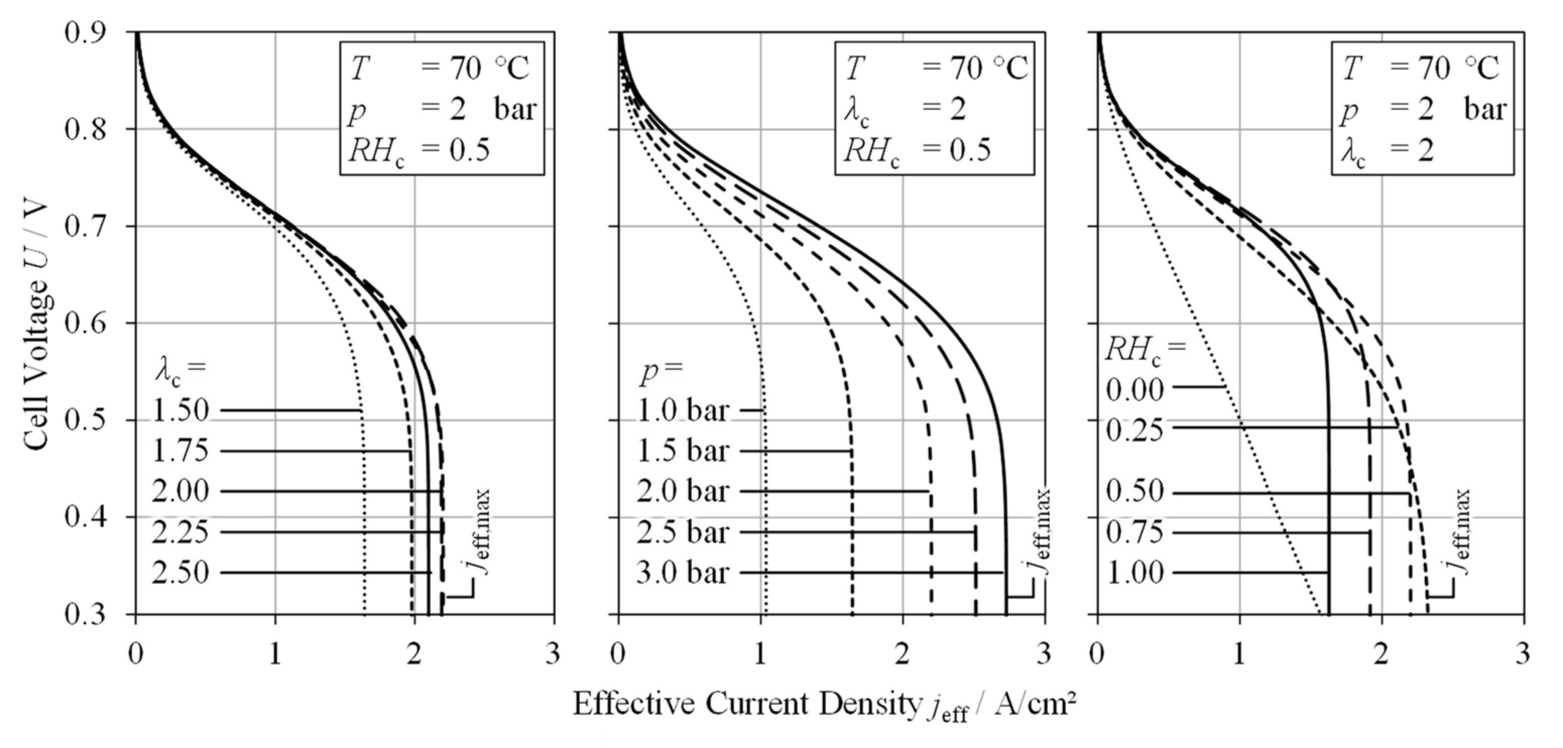
Multiple approaches to PEM FC powertrain component modeling have been presented in the literature, ranging from simple empirical models (e.g., [2,15]) to three-dimensional computational fluid dynamics simulations (3D CFD, e.g., [16,17]). For the following investigation, semi-empirical models are used. Basic relationships are described by physical equations while the exact component operating behavior is tuned using empirical data.

2.1. PEM FC Model

The efficiency of a PEM FC highly depends on the concentrations of hydrogen, oxygen and water in the reaction zones (cathode and anode catalyst layers CCL and ACL) as well as on the conductivity of the polymer electrolyte membrane. In order to resolve these parameters along the gas channels (defined by the bipolar plates) and in the thickness direction of the membrane electrode assembly (MEA), the two-dimensional finite volume model shown in Figure 1 is introduced.

The gas channels are discretized into i_k elements. The thickness of the gas diffusion layers (GDL) and the PEM are divided into i_GDL and i_mem elements, respectively. i_k = 20 and i_GDL = i_mem = 5 are reasonable starting points.

The time derivative d/dt for the amount of substance n in one gas channel element with volume V can be written as follows:

$${\displaystyle \frac{dn}{dt}}={\displaystyle \frac{V}{RT}}{\displaystyle \frac{dp}{dt}}-T^2{\displaystyle \frac{pV}{ R}}{\displaystyle \frac{dT}{dt}}\hspace{1em}\mathrm{w}\mathrm{i}\mathrm{t}\mathrm{h}\hspace{1em}V,R=\mathrm{c}\mathrm{o}\mathrm{n}\mathrm{s}\mathrm{t}.$$

(1)

R = 8.341 J/mol·K is the ideal gas constant, p is the pressure and T is the temperature in the gas channel element [18]. Conservation of mass yields the following relations for the molar flow rates entering and exiting the gas channel element ṅ_in and ṅ_out:

$$\begin{array}{c}{\displaystyle \frac{dn}{dt}}={\dot{n}}_{\mathrm{i}\mathrm{n}}-{\dot{n}}_{\mathrm{o}\mathrm{u}\mathrm{t}}\\ \mathrm{w}\mathrm{i}\mathrm{t}\mathrm{h}\hspace{1em}{\sum }_{\mathrm{i}}{\dot{n}}_{\mathrm{o}\mathrm{u}\mathrm{t},\mathrm{i}}={\dot{n}}_{\mathrm{o}\mathrm{u}\mathrm{t}},\hspace{1em}{\dot{n}}_{\mathrm{o}\mathrm{u}\mathrm{t},\mathrm{i}}=x_{\mathrm{i}}{\dot{n}}_{\mathrm{o}\mathrm{u}\mathrm{t}},\hspace{1em}{x}_{\mathrm{i}}={\displaystyle \frac{n_{\mathrm{i}}}{n}}\hspace{1em}\mathrm{i}={\mathrm{H}}_2, {\mathrm{O}}_2, {\mathrm{H}}_2\mathrm{O}, {\mathrm{N}}_2\end{array}$$

(2)

An ideal mixing of all substances (Hydrogen H₂, Oxygen O₂, Water H₂O and Nitrogen N₂) is assumed in the channel elements. This way, the exiting molar flow rates of the different substances ṅ_out,i are linked to their respective molar fractions x_i. Pressure loss in the gas channels is estimated using the Darcy–Weisbach equation [19]:

$${\displaystyle \frac{dp}{dz}}={\displaystyle \frac{\Lambda }{\rho d_{\mathrm{h}}}}{c}^2={\displaystyle \frac{\Lambda }{\rho d_{\mathrm{h}}}}{\left({\displaystyle \frac{4\dot{n}RT}{p{d}_{\mathrm{h}}^2\pi }}\right)}^2\hspace{1em}\mathrm{w}\mathrm{i}\mathrm{t}\mathrm{h}\hspace{1em}{d}_h={\displaystyle \frac{4A}{\chi }}$$

(3)

Λ is the experimentally determined friction coefficient, ρ is the gas density and d_h is the hydraulic diameter of the gas channel derived from its cross section A and wetted perimeter χ.

Diffusion within the GDL and the PEM is governed by Fick’s diffusion law [20]. Assuming diffusion to predominantly occur in the x-direction (dur to a high aspect ratio of discretization elements and dominant concentration gradient in x-direction dc^/dx >> dc^/dz), the general representation of the molar flux density ṅ” is converted to the following simplified representation [21]:

$${\dot{n}}^{″}=-D\nabla c\hspace{1em}\to \hspace{1em}{\dot{n}}_{\mathrm{x}}^{″}=-D{\displaystyle \frac{d\mathrm{c}}{dx}}\hspace{1em},\hspace{1em}{\dot{n}}_{\mathrm{z}}^{″}=0$$

(4)

D is the diffusion coefficient. Diffusion is assumed to occur in the x-direction only. Substance transport in the z-direction is achieved via the gas channels.

If liquid water is formed in the GDL, oxygen diffusion is impeded. Building on [22,23,24,25], the effective oxygen diffusion coefficient in the GDL D_O2,eff is written as a function of wet GDL porosity ϕ_w:

$$\begin{array}{c}{\displaystyle \frac{1}{D_{{\mathrm{O}}_2,\mathrm{e}\mathrm{f}\mathrm{f}}}}=\left({\displaystyle \frac{1-{\varphi }_{\mathrm{w}}}{D_{{\mathrm{O}}_2}}}+{\displaystyle \frac{{\varphi }_{\mathrm{w}}}{D_{{\mathrm{O}}_2,\mathrm{w}}}}\right){\varphi }_{\mathrm{G}\mathrm{D}\mathrm{L}}^{-1.5}\\ \mathrm{w}\mathrm{i}\mathrm{t}\mathrm{h}\hspace{1em}{\varphi }_{\mathrm{w}}={\displaystyle \frac{V_{\mathrm{w}}}{V_{\mathrm{G}\mathrm{D}\mathrm{L}}}}={\varphi }_{\mathrm{G}\mathrm{D}\mathrm{L}}{\displaystyle \frac{p_{\mathrm{w}}{M}_{{\mathrm{H}}_2\mathrm{O}}}{{\rho }_{\mathrm{w}}RT}}\hspace{1em},\hspace{1em}{p}_{\mathrm{w}}=p_{{\mathrm{H}}_2\mathrm{O}}-p_{\mathrm{s}}\hspace{1em},\hspace{1em}{\varphi }_{\mathrm{G}\mathrm{D}\mathrm{L}}={\displaystyle \frac{V_{\mathrm{p}\mathrm{o}\mathrm{r}}}{V_{\mathrm{G}\mathrm{D}\mathrm{L}}}}\end{array}$$

(5)

D_O₂ and D_O₂,w are the diffusion coefficients of oxygen in air and liquid water. p_w is the difference between the partial pressure p_H₂O and the saturation pressure p_s of water. ϕ_GDL is the porosity of the dry GDL (ratio of pore volume V_por and GDL bulk volume V_GDL). ρ_w is the density of liquid water.

The water content λ_mem is a measure for the water absorbed per sulfonic acid end group within the PEM:

$${\lambda }_{\mathrm{m}\mathrm{e}\mathrm{m}}={\displaystyle \frac{n_{{\mathrm{H}}_2\mathrm{O}}}{n_{\mathrm{S}{\mathrm{O}}_3^{-}}}}=c_{{\mathrm{H}}_2\mathrm{O}}{\displaystyle \frac{M_{\mathrm{m}\mathrm{e}\mathrm{m}}}{{\rho }_{\mathrm{m}\mathrm{e}\mathrm{m}}}}$$

(6)

M_mem and ρ_mem are the average molecular weight and density of the PEM. For Nafion, M_mem = 544 g/mol and ρ_mem = 1.6 kg/m³ can be assumed (cf. [26,27]). Water absorption on the PEM surfaces is described as a function of relative humidity RH by the experimentally determined sorption isotherms introduced in [28]:

$$\begin{array}{c}{\lambda }_{\mathrm{m}\mathrm{e}\mathrm{m}}=0.3+6RH\left[1-\tanh \left(RH-0.5\right)\right]+3.9\sqrt{RH}\left[1-\tanh \left({\displaystyle \frac{RH-0.89}{0.23}}\right)\right]\\ \mathrm{w}\mathrm{i}\mathrm{t}\mathrm{h}\hspace{1em}\mathrm{}RH={\displaystyle \frac{x_{{\mathrm{H}}_2\mathrm{O}}p}{p_{\mathrm{s}}}}=0\dots 3\end{array}$$

(7)

The relation derived in [28] (based on data from [29]) is used to describe the water diffusion coefficient in the PEM D_H₂O,mem:

$$D_{{\mathrm{H}}_2\mathrm{O},\mathrm{m}\mathrm{e}\mathrm{m}}=4.1·{10}^{-10}{\left({\displaystyle \frac{{\lambda }_{\mathrm{m}\mathrm{e}\mathrm{m}}}{25}}\right)}^{0.15}\left[1+\tanh \left({\displaystyle \frac{{\lambda }_{\mathrm{m}\mathrm{e}\mathrm{m}}-2.5}{1.4}}\right)\right]{\displaystyle \frac{{\mathrm{m}}^2}{\mathrm{s}}}$$

(8)

The area-specific PEM resistance r_mem is calculated by integrating the empiric correlation for PEM conductivity σ_mem taken from [28] over the PEM thickness x_mem:

$$r_{\mathrm{m}\mathrm{e}\mathrm{m}}={\int }_0^{x_{\mathrm{m}\mathrm{e}\mathrm{m}}}{\sigma }_{\mathrm{m}\mathrm{e}\mathrm{m}}^{-1}dx\hspace{1em}\mathrm{w}\mathrm{i}\mathrm{t}\mathrm{h}\hspace{1em}{\sigma }_{\mathrm{m}\mathrm{e}\mathrm{m}}=\left\{\begin{array}{cc}0& {\lambda }_{\mathrm{m}\mathrm{e}\mathrm{m}}<1.25\\ \left(0.574{\lambda }_{\mathrm{m}\mathrm{e}\mathrm{m}}-0.72\right){\displaystyle \frac{1}{\mathsf{\Omega }\mathrm{c}\mathrm{m}}}\mathrm{}& {\mathsf{\lambda }}_{\mathrm{m}\mathrm{e}\mathrm{m}}\ge 1.25\end{array}\right.$$

(9)

According to [21], the cell voltage U can be written as a function of the local current density j (the ratio of the local cell current I and cell area A_z):

$$\begin{array}{c}U=U_{\mathrm{r}\mathrm{e}\mathrm{v}}-\left(r_{\mathrm{B}\mathrm{P}}+r_{\mathrm{m}\mathrm{e}\mathrm{m}}\right)j-b\left[\mathsf{\Psi }\left({\displaystyle \frac{j}{j^{*}}}\right)\ln \left({\displaystyle \frac{j}{j^{*}}}\right)-\ln \left({\displaystyle \frac{c_{{\mathrm{O}}_2}}{c_{{\mathrm{O}}_2,\mathrm{r}\mathrm{e}\mathrm{f}}}}{\displaystyle \frac{x_{\mathrm{C}\mathrm{C}\mathrm{L}}{j}_0}{j^{*}}}\mathrm{}\right)-\ln \left(1-{\displaystyle \frac{j}{j_{\mathrm{m}\mathrm{a}\mathrm{x}}\mathrm{}}}\right)\right]\\ \mathrm{w}\mathrm{i}\mathrm{t}\mathrm{h}\hspace{1em}j={\displaystyle \frac{dI}{d{A}_{\mathrm{z}}}}\hspace{1em},\hspace{1em}{U}_{\mathrm{r}\mathrm{e}\mathrm{v}}=-{\displaystyle \frac{\Delta g_{\mathrm{f}}}{2F}}=1.23 \mathrm{V}\hspace{1em},\hspace{1em}b={\displaystyle \frac{RT}{{\alpha }_{0}F}}\mathrm{}\mathrm{},\hspace{1em}{j}^{*}={\displaystyle \frac{2{\sigma }_{\mathrm{C}\mathrm{C}\mathrm{L}}b}{x_{\mathrm{C}\mathrm{C}\mathrm{L}}}}\\ \Psi \left({\displaystyle \frac{j}{j^{*}}}\right)=1+{\displaystyle \frac{{\left(\frac{j}{j^{*}}\right)}^2}{1+{\left(\frac{j}{j^{*}}\right)}^2}},\hspace{1em}{j}_{\mathrm{m}\mathrm{a}\mathrm{x}}={\displaystyle \frac{4F{D}_{{\mathrm{O}}_2,\mathrm{e}\mathrm{f}\mathrm{f}}{c}_{{\mathrm{O}}_2}}{x_{\mathrm{G}\mathrm{D}\mathrm{L}}}}\end{array}$$

(10)

U_ref is the reversible cell voltage (Nernst voltage) derived from Gibb´s free enthalpy of the hydrogen reaction Δg_f and the Faraday constant F. r_BP is the lumped area-specific (ohmic) resistance of the bipolar plates and the GDL (incl. contact resistances). b is the Tafel slope of the hydrogen reaction (dependent on the reaction symmetry factor α₀ = 0.5) and j* is the characteristic current density depending on CCL conductivity σ_CCL and thickness x_CCL. j₀ is the exchange current density and c_O₂ is the reference oxygen concentration for which j₀ is determined. The limiting current density j_max is a function of the cathode gas channel oxygen concentration c_O₂ and GDL thickness x_GDL. The blending function Ψ is used to switch between the solution regimes for low and high current density.

Within the FC stack, all i_c cells are considered equal. Accordingly, stack voltage U_stack, power P_stack and efficiency η_stack can be calculated as follows:

$$U_{\mathrm{s}\mathrm{t}\mathrm{a}\mathrm{c}\mathrm{k}}=i_{\mathrm{c}}U,\hspace{1em}{P}_{\mathrm{s}\mathrm{t}\mathrm{a}\mathrm{c}\mathrm{k}}=i_{\mathrm{c}}UI,\hspace{1em}{\eta }_{\mathrm{s}\mathrm{t}\mathrm{a}\mathrm{c}\mathrm{k}}={\eta }_{\mathrm{u}}={\displaystyle \frac{U}{U_{\Delta h_{\mathrm{f},\mathrm{u}}}}}\hspace{1em}\mathrm{w}\mathrm{i}\mathrm{t}\mathrm{h}\hspace{1em}{U}_{\Delta h_{\mathrm{f},\mathrm{u}}}={\displaystyle \frac{-\Delta h_{\mathrm{f},\mathrm{u}}}{2F}}=1.25 \mathrm{V}$$

(11)

Cell efficiency η_u is the quotient of cell voltage U and lower heating voltage U_Δhf,u (derived from the lower formation enthalpy of the hydrogen reaction Δh_f,u). The values given for U_rev and U_Δhf,u are calculated at standard temperature and pressure T_ref = 25 °C and p_ref = 1 bar [2].

The molar reaction rates for oxygen ṅ_reac,O₂, water ṅ_reac,H₂O and hydrogen ṅ_reac,H₂ are calculated as

$$2d{\dot{n}}_{\mathrm{r}\mathrm{e}\mathrm{a}\mathrm{c},{\mathrm{O}}_2}=d{\dot{n}}_{\mathrm{r}\mathrm{e}\mathrm{a}\mathrm{c},{\mathrm{H}}_2\mathrm{O}}=-d{\dot{n}}_{\mathrm{r}\mathrm{e}\mathrm{a}\mathrm{c},{\mathrm{H}}_2}={\displaystyle \frac{jd{A}_{\mathrm{z}}}{2F}}$$

(12)

and superimposed on the diffusion equations as sink- and source-terms. Based on the oxygen and hydrogen molar flow rates entering the cathode and anode ṅ_c,O₂ and ṅ_a,H₂, the respective stoichiometries λ_c and λ_a are defined as follows [2]:

$${\lambda }_{\mathrm{c}}={\dot{n}}_{\mathrm{c},{\mathrm{O}}_2}{\displaystyle \frac{4F}{I}} ,\hspace{1em}{\lambda }_{\mathrm{a}}={\dot{n}}_{\mathrm{a},{\mathrm{H}}_2}{\displaystyle \frac{2F}{I}}\hspace{1em}\mathrm{w}\mathrm{i}\mathrm{t}\mathrm{h}\hspace{1em}I=\int j{dA}_{\mathrm{z}}\hspace{1em},\hspace{1em}{j}_{\mathrm{e}\mathrm{f}\mathrm{f}}={\displaystyle \frac{I}{A_{\mathrm{z}}}}$$

(13)

The time-dependent (transient) solution of the differential equation system is determined using the Euler–Cauchy method. For a co-flow arrangement of the cathode and anode gas channels, the stationary solution can be determined in a direct-marching approach. For a cross-flow arrangement, a relaxation approach must be used.

Figure 2 shows the stationary results of the introduced PEM FC model for a variation of cathode stoichiometry λ_c, relative humidity at cathode inlet RH_c and operating pressure p. Cathode and anode side humidity and pressure are set equal, and a co-flow arrangement is assumed. The model (i.e., the calibration parameters of Equation (10)) is validated against stack test bench and vehicle measurements performed in [30,31].

The exemplary model results of Figure 2 can be used to assess the influence of operating boundary conditions on PEM FC performance.

The effective current density j_eff is determined by integrating j along the gas channel direction (inlet: z = 0, outlet: z = z_max). The effective limiting current density j_eff,max is derived accordingly:

$$\begin{array}{c}{j}_{\mathrm{e}\mathrm{f}\mathrm{f}}={\displaystyle \frac{1}{z_{\mathrm{m}\mathrm{a}\mathrm{x}} }}{\int }_{z=0}^{z_{\mathrm{m}\mathrm{a}\mathrm{x}}}jdz\hspace{1em},\hspace{1em}{j}_{\mathrm{e}\mathrm{f}\mathrm{f},\mathrm{m}\mathrm{a}\mathrm{x}}={\displaystyle \frac{1}{z_{\mathrm{m}\mathrm{a}\mathrm{x}}}}{\int }_{z=0}^{z_{\mathrm{m}\mathrm{a}\mathrm{x}}}{j}_{\mathrm{m}\mathrm{a}\mathrm{x}}dz\\ \mathrm{w}\mathrm{i}\mathrm{t}\mathrm{h}\hspace{1em}{j}_{\mathrm{m}\mathrm{a}\mathrm{x}}={\displaystyle \frac{4F{D}_{{\mathrm{O}}_2,\mathrm{e}\mathrm{f}\mathrm{f}}{c}_{{\mathrm{O}}_2}}{x_{\mathrm{G}\mathrm{D}\mathrm{L}}}}\end{array}$$

(14)

Increasing λ_c yields higher c_O₂, especially in downstream gas channel elements. This results in increasing limiting current densities and decreasing overpotential (higher cell voltage). For excessive λ_c (dependent on the model calibration; here, λ_c ≥ 2.25), product water is transported out of the cell too quickly by the high gas flow rates. The PEM cannot be sufficiently humidified, σ_mem decreases and cell voltage is reduced. This effect (known as cell dry-out) should be avoided to maximize cell performance and lifetime.

To ensure good proton conductivity, a sufficiently high and homogeneous humidification of the PEM by means of cathode inlet air humidification is vital. For RH_c = 0, the PEM is only humidified by the product water; i.e., for co-flow arrangements, this yields a low j_eff in upstream cell areas (due to low PEM conductivity, r_mem → ∞) and a high j_eff in downstream cell areas which compensate for the insufficiently humidified sections (while exhibiting high overpotential). For the example given in Figure 2, reasonable proton conductivity is achieved for RH_c > 25%. In general, the required humidity level at cathode air inlet highly depends on stack and cell design as well as on the operating strategy (cf. Section 3.1) [2,32].

For RH_c ↑, the current density distribution is smoothed out (a more uniform PEM conductivity over the entire gas channel length → a reduction of cell areas with elevated local current density and high overpotential), and cell performance is improved. If RH_c is too high, gas channel oxygen is displaced by water vapor and liquid water hinders oxygen diffusion within the GDL (cf. Equation (5)), resulting in decreased cell performance, an effect known as cell flooding. Figure 2 clearly shows a decreasing cell voltage for RH_c > 50% at a medium and high effective current density j_eff ≥ 1.2 A/cm², highlighting this effect.

Gas channel oxygen concentration is directly proportional to operating pressure. Furthermore, relative humidity increases with p for constant water molar fraction x_H₂O:

$$c_{{\mathrm{O}}_2}={\displaystyle \frac{x_{{\mathrm{O}}_2}p}{RT}}\hspace{1em},\hspace{1em}RH={\displaystyle \frac{x_{{\mathrm{H}}_2\mathrm{O}}p}{p_{\mathrm{s}}}}$$

(15)

For c_O₂ ↑, cell overpotential is reduced and limiting current density is increased. RH ↑ promotes proton conductivity which further reduces cell overpotential. Overall, p ↑ significantly increases cell efficiency and power density.

The presented model accurately predicts PEM FC performance over a wide range of operating boundary conditions. The physically based modeling approach allows for reliable measurement data extrapolation.

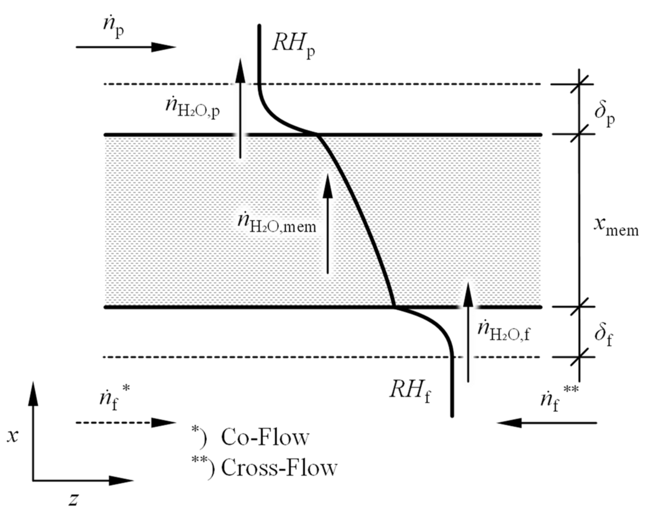
2.2. Membrane Humidifier Model

The membrane humidifier model uses the same principles as the PEM FC model. The permeate (dry side, index _p) and feed (wet side, index _f) gas channels are discretized into i_k elements. The humidifier membrane is discretized into i_mem elements. i_k = 20 and i_mem = 10 are usually sufficient to correctly resolve humidifier behavior within the expected operating range.

Figure 3 shows the molar flow rates in the permeate and feed side gas channels ṅ_p and ṅ_f as well as the water transport across the humidifier membrane ṅ_H₂O,mem and the respective boundary layers δ_p and δ_f.

According to [33], water molar flux density across the boundary layers on permeate and feed side ṅ”_H₂O,i can be written as follows:

$${\dot{n}}_{{\mathrm{H}}_2\mathrm{O},\mathrm{i}}^{\prime \prime }={\displaystyle \frac{d{\dot{n}}_{{\mathrm{H}}_2\mathrm{O},\mathrm{i}}}{dA}}=-h_{\mathrm{m}}^{*}\Delta c_{{\mathrm{H}}_2\mathrm{O},\mathrm{i}}\hspace{1em}\mathrm{w}\mathrm{i}\mathrm{t}\mathrm{h}\hspace{1em}\mathrm{i}=\mathrm{p},\mathrm{f}$$

(16)

Δc_H₂O is the concentration gradient across the respective boundary layer. To determine the mass transfer coefficient h^*_m, the correlation from [34] h_m must be corrected for evaporation and condensation on the membrane surfaces [33]:

$$\begin{array}{c}\mathrm{E}\mathrm{v}\mathrm{a}\mathrm{p}\mathrm{o}\mathrm{r}\mathrm{a}\mathrm{t}\mathrm{i}\mathrm{o}\mathrm{n}:\hspace{1em}{h}_{\mathrm{m}}^{*}={\displaystyle \frac{1}{\exp \left(\frac{{\dot{n}}_{{\mathrm{H}}_2\mathrm{O}}^{\prime \prime }}{h_{\mathrm{m}}}\right)-1}}\hspace{1em},\hspace{1em}\mathrm{C}\mathrm{o}\mathrm{n}\mathrm{d}\mathrm{e}\mathrm{n}\mathrm{s}\mathrm{a}\mathrm{t}\mathrm{i}\mathrm{o}\mathrm{n}:\hspace{1em}{h}_{\mathrm{m}}^{*}={\displaystyle \frac{1}{1-\exp \left(\frac{{\dot{n}}_{{\mathrm{H}}_2\mathrm{O}}^{\prime \prime }}{h_{\mathrm{m}}}\right)}}\\ \mathrm{w}\mathrm{i}\mathrm{t}\mathrm{h}\hspace{1em}{h}_{\mathrm{m}}=\mathrm{}0.023R{e}^{0.8}S{c}^{0.4}{\displaystyle \frac{D_{{\mathrm{H}}_2\mathrm{O},\mathrm{a}\mathrm{i}\mathrm{r}}}{d_{\mathrm{h}}}}\mathrm{}[34]\hspace{1em},\hspace{1em}Re={\displaystyle \frac{c{d}_{\mathrm{h}}}{\nu }}\hspace{1em},\hspace{1em}Sc={\displaystyle \frac{\nu }{D_{{\mathrm{H}}_2\mathrm{O},\mathrm{a}\mathrm{i}\mathrm{r}}}}\hspace{1em},\hspace{1em}\nu ={\displaystyle \frac{\eta }{\rho }}\end{array}$$

(17)

Re and Sc are the Reynolds and Schmidt number, d_h is the hydraulic diameter of the humidifier gas channel, D_H₂O,air is the self-diffusion coefficient of water vapor in air and ν and η are the kinematic and dynamic viscosities, respectively. The correlations from [33,35] are used for D_H₂O,air and η:

$$D_{{\mathrm{H}}_2\mathrm{O},\mathrm{a}\mathrm{i}\mathrm{r}}=22.5·{10}^6{\left({\displaystyle \frac{T}{273.15 \mathrm{K}}}\right)}^{1.8}\left({\displaystyle \frac{1 \mathrm{b}\mathrm{a}\mathrm{r}}{p}} \right)\hspace{1em},\hspace{1em}\eta =17.16{\displaystyle \frac{384 \mathrm{K}}{T+111 \mathrm{K}}}{\left({\displaystyle \frac{T}{111 \mathrm{K}}}\right)}^{1.5}\mathsf{\mu }\mathrm{P}\mathrm{a}\mathrm{s}$$

(18)

Equivalent to the PEM FC model, the transient solution of the differential equation system is determined numerically on the discretization grid. To determine the stationary solution, the integral water diffusion coefficient of the humidifier membrane D_H₂O,eff is found by integrating Equation (8) over the membrane thickness x_mem:

$$\begin{array}{c}{\dot{n}}_{{\mathrm{H}}_2\mathrm{O},\mathrm{m}\mathrm{e}\mathrm{m}}^{\mathrm{″}}=D_{{\mathrm{H}}_2\mathrm{O},\mathrm{e}\mathrm{f}\mathrm{f}}\frac{c_{{\mathrm{H}}_2\mathrm{O},\mathrm{f}}-c_{{\mathrm{H}}_2\mathrm{O},\mathrm{p}}}{x_{\mathrm{m}\mathrm{e}\mathrm{m}}} \mathrm{w}\mathrm{i}\mathrm{t}\mathrm{h} c_{{\mathrm{H}}_2\mathrm{O},\mathrm{i}}={\lambda }_{\mathrm{m}\mathrm{e}\mathrm{m},\mathrm{i}}\frac{{\rho }_{\mathrm{m}\mathrm{e}\mathrm{m}}}{M_{\mathrm{m}\mathrm{e}\mathrm{m}}} \mathrm{f}\mathrm{r}\mathrm{o}\mathrm{m} \mathrm{E}\mathrm{q}\mathrm{u}\mathrm{a}\mathrm{t}\mathrm{i}\mathrm{o}\mathrm{n} (6)\\ D_{{\mathrm{H}}_2\mathrm{O},\mathrm{e}\mathrm{f}\mathrm{f}}=\frac{1}{x_{\mathrm{m}\mathrm{e}\mathrm{m}}}{\int }_{x=0}^{x_{\mathrm{m}\mathrm{e}\mathrm{m}}}{D}_{{\mathrm{H}}_2\mathrm{O},\mathrm{m}\mathrm{e}\mathrm{m}}dx, D_{{\mathrm{H}}_2\mathrm{O},\mathrm{m}\mathrm{e}\mathrm{m}}\left({\lambda }_{\mathrm{m}\mathrm{e}\mathrm{m}}\right) \mathrm{f}\mathrm{r}\mathrm{o}\mathrm{m} \mathrm{E}\mathrm{q}\mathrm{u}\mathrm{a}\mathrm{t}\mathrm{i}\mathrm{o}\mathrm{n} (8) , {\lambda }_{\mathrm{m}\mathrm{e}\mathrm{m}} \mathrm{f}\mathrm{r}\mathrm{o}\mathrm{m} \mathrm{E}\mathrm{q}\mathrm{u}\mathrm{a}\mathrm{t}\mathrm{i}\mathrm{o}\mathrm{n} (7)\end{array}$$

(19)

The membrane humidifier model is calibrated using experimental data acquired on a component test bench by [32]. Within a statistical design of experiments approach, mass flow rates, pressures, temperatures and inlet relative humidities were varied on the permeate and feed side (in a cross-flow arrangement). Water transfer across the membrane ṁ_H₂O was calculated based on the humidifier outlet states. The model tuning parameters (membrane thickness, surface area and density) are selected to minimize the average quadratic error between the model and measurement results.

Figure 4 exemplarily shows the stationary solution of the membrane humidifier model. Here, permeate and feed side relative humidities are investigated for varying mass flow rates ṁ_p = ṁ_f = ṁ in a cross-flow arrangement. Figure 4 also shows a comparison between the measurement and model results for a mass flow rate and operating pressure variation (ṁ_p = ṁ_f = ṁ, p_p = p_f = p). For this, a cross-section of the eight-dimensional experimental design space was determined using radial basis function interpolation (cf. [36]).

For lower ṁ (longer gas residence time in the humidifier), the specific water mass transfer increases. The permeate side outlet relative humidity RH_p,out increases and the feed side outlet relative humidity RH_f,out decreases accordingly. For ṁ ↑, the specific water mass transfer is reduced (shorter gas residence time in humidifier), and RH_p,out drops accordingly. With p ↑, the relative humidity increases for x_H₂O = const. (cf. Equation (15)). This yields a higher RH_p,out even for operating points with lower water mass transfer, underlining the importance of operating pressure for PEM FC system water management.

For ṁ → 0, RH_p,out = RH_f,in holds for the cross-flow arrangement, whereas for a co-flow arrangement, only RH_p,out = RH_f,out ≤ RH_f,in can be reached. In general, significantly higher specific water mass transfer rates are achieved for the cross-flow arrangement due to higher average values for the concentration gradient and diffusion coefficient.

Overall, the measurement and model show good agreement over the entire operating range. Deviations towards high ṁ and low p can be partially explained by measurement inaccuracies and interpolation errors originating from low measurement point density in this region (cf. [32]).

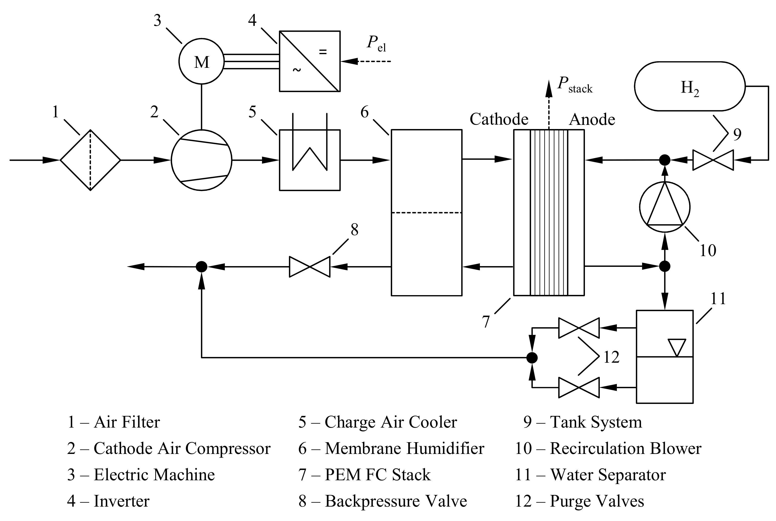
2.3. PEM FC System Model

In the following section, the presented component models are merged into a simulation of the PEM FC system as laid out in Figure 5. The system model is used to determine the optimum operating strategy of the cathode air compressor. Finally, the influence of PEM FC stack and membrane humidifier sizing on the optimum compressor operating strategy as well as the provisions required to compensate for cell ageing are investigated.

The operating behavior of the cathode air compressor is described by a performance map. The charge air cooler ensures that the maximum allowable inlet temperature of the membrane humidifier and PEM FC stack is not exceeded. The anode loop (tank system, recirculation blower, water separator and purge valves) is controlled to ensure a sufficient stoichiometry and satisfactory PEM water content. Cathode stoichiometry and operating pressure are determined by the air compressor operating speed and backpressure valve position.

To determine the stationary solution of the system model, a relaxation approach is used. Starting from an initialization with ambient conditions, component outlet states are repeatedly imposed as inlet states of downstream components until convergence is achieved. System model performance is validated against vehicle measurements performed in [30] (stationary and transient chassis dynamometer tests). A good agreement between model results and measurement data is achieved for the pressures, temperatures and relative humidities over the entire operating range.

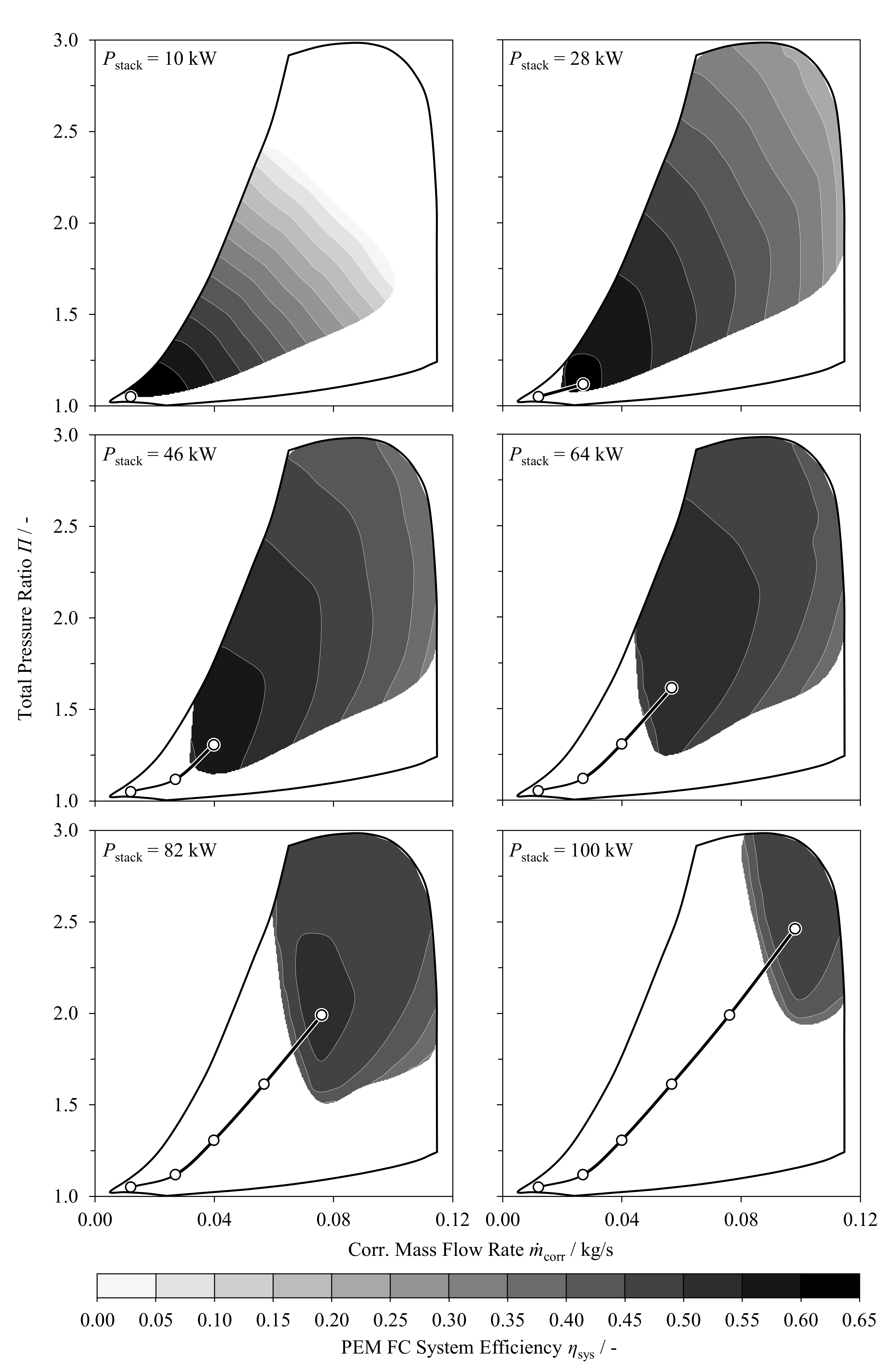
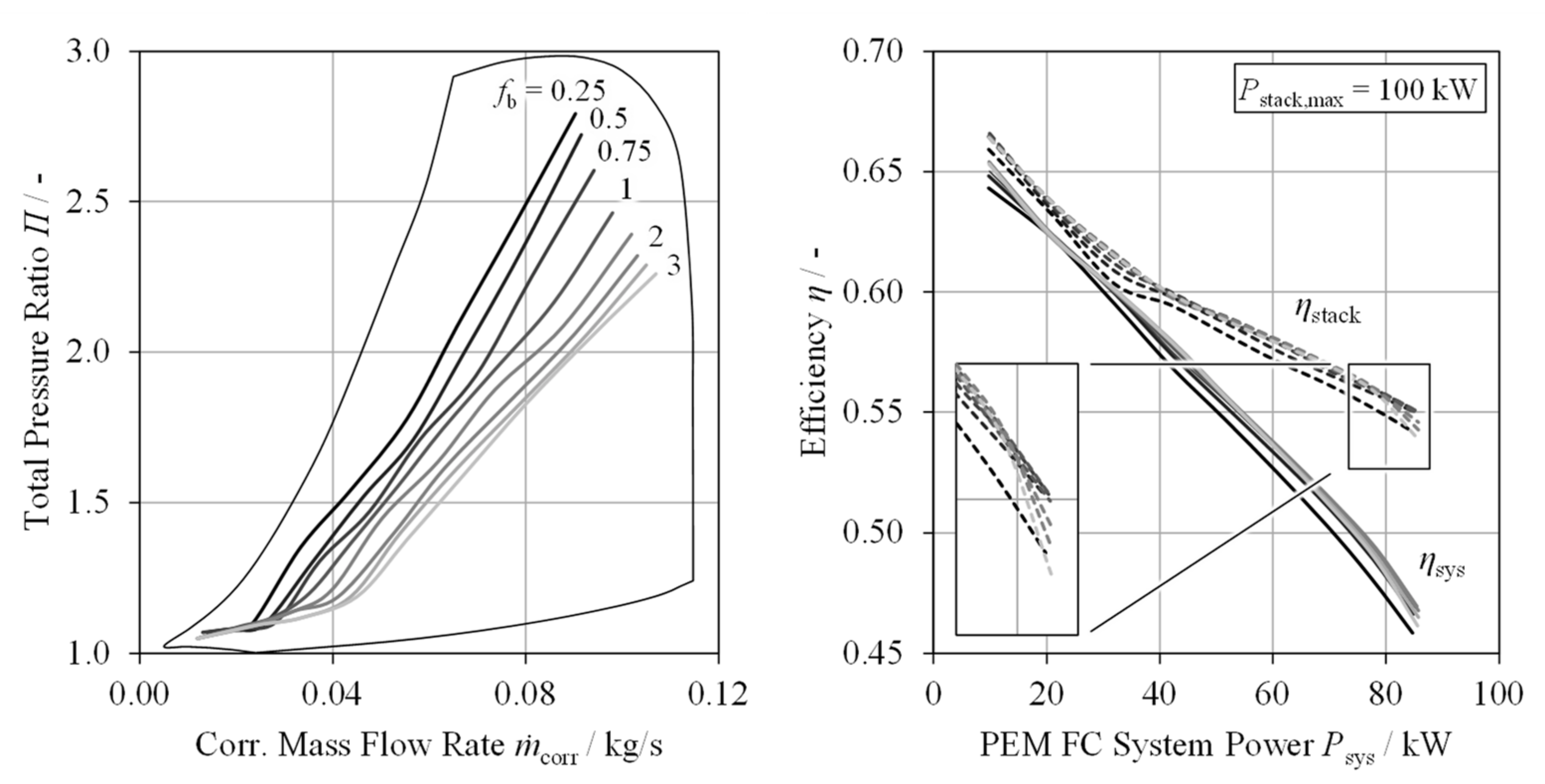
3. Operating Strategy Optimization

For the given stage inlet thermodynamic conditions (total temperature and pressure T_t0 and p_t0), the compressor operating point is defined by the corrected mass flow rate ṁ_corr and total pressure ratio Π (total pressure at stage outlet p_t6). The compressor performance map (determined from numerical estimates or measurements) yields the corresponding corrected and physical compressor speed n_corr and n as well as the isentropic compressor efficiency η_s:

$${\dot{m}}_{\mathrm{c}\mathrm{o}\mathrm{r}\mathrm{r}}=\dot{m}{\displaystyle \frac{p_{\mathrm{r}\mathrm{e}\mathrm{f}}}{p_{\mathrm{t}0}}}\sqrt{{\displaystyle \frac{T_{\mathrm{t}0}}{T_{\mathrm{r}\mathrm{e}\mathrm{f}}}}}\hspace{1em},\hspace{1em}\Pi ={\displaystyle \frac{p_{\mathrm{t}6}}{p_{\mathrm{t}0}}}\hspace{1em}\stackrel{\begin{array}{c}\mathrm{Perf}.\\ \mathrm{Map}\end{array}}{\to }\hspace{1em}{n}_{\mathrm{c}\mathrm{o}\mathrm{r}\mathrm{r}}=n\sqrt{{\displaystyle \frac{T_{\mathrm{r}\mathrm{e}\mathrm{f}}}{T_{\mathrm{t}0}}}}\hspace{1em},\hspace{1em}{\eta }_{\mathrm{s}}={\displaystyle \frac{T_{\mathrm{t}0}\left( {\Pi }^{\frac{\kappa -1}{\kappa }}-1\right)}{T_{\mathrm{t}6}-T_{\mathrm{t}0}}}$$

(20)

For each stack power level, the compressor operating point (ṁ_corr, Π) maximizing the PEM FC system efficiency η_sys shall be found:

$${\underset{{\dot{m}}_{\mathrm{corr}},\Pi }{\max }}_{|P_{\mathrm{stack}}}{\eta }_{\mathrm{s}\mathrm{y}\mathrm{s}}\hspace{1em}\mathrm{w}\mathrm{i}\mathrm{t}\mathrm{h}\hspace{1em}{\eta }_{\mathrm{s}\mathrm{y}\mathrm{s}}={\displaystyle \frac{P_{\mathrm{s}\mathrm{t}\mathrm{a}\mathrm{c}\mathrm{k}}-P_{\mathrm{e}\mathrm{l}}}{\frac{P_{\mathrm{s}\mathrm{t}\mathrm{a}\mathrm{c}\mathrm{k}}}{{\eta }_{\mathrm{s}\mathrm{t}\mathrm{a}\mathrm{c}\mathrm{k}}}}}\hspace{1em},\hspace{1em}{P}_{\mathrm{e}\mathrm{l}}={\displaystyle \frac{1}{{\eta }_{\mathrm{e}\mathrm{f}\mathrm{f}}}}\underset{{=P}_{\mathrm{s}}}{\underbrace{\dot{m}{c}_{\mathrm{p}}{T}_{\mathrm{t}0}\left({\Pi }^{{\displaystyle \frac{\kappa -1}{\kappa }}}-1\right)}}$$

(21)

η_sys considers the stack power P_stack and efficiency η_stack as well as the electric power consumption of the cathode air compressor P_el. P_el is a function of the isentropic compressor power P_s. The isentropic compressor efficiency η_s, the mechanical efficiency of the air bearing system and the efficiency of the electric machine (incl. the inverter) are summarized in the effective compressor efficiency η_eff. The power consumption of the additional balance of plant components (recirculation blower, coolant pumps, etc.) is neglected here for reasons of simplicity but can be easily incorporated, if required.

Connecting the optimum compressor operating points determined according to Equation (21) for all P_stack yields the system efficiency optimal compressor operating strategy (optimum operating line) shown in Figure 6.

For low P_stack (low j_eff), the influence of the cathode stoichiometry and operating pressure on stack efficiency is marginal (cf. cell voltage in Figure 2). For optimum η_sys, the compressor operating point should therefore be selected in the lower left-hand map range. The minimum compressor power is limited by the minimum operating speed (sufficient distance to air bearing lift-off speed) and the minimum pressure ratio required to overcome the pressure losses of the cathode air path. With ṁ_corr ↑ and Π ↑, P_el increases, and η_sys decreases until P_stack = P_el and P_sys = 0. Beyond this point, η_sys = 0 is set by definition.

Each stack target power P_stack,target requires a combination of the minimum corrected mass flow rate ṁ_corr,min and total pressure ratio Π_min (cf. also Section 3.2). Below this limit curve, the stack target power cannot be reached; P_stack,max < P_stack,target. Here, η_sys = 0 is set. The feasible compressor map range is limited by cell dry-out towards the bottom right, cell flooding towards the top and insufficient CCL oxygen concentration towards the bottom. With P_stack,target ↑, the feasible map range is shifted to higher ṁ_corr and Π.

For ṁ_corr ↑ and Π ↑, stack efficiency is improved (cf. Figure 2) and P_el increases. Consequently, compressor power, PEM/GDL water content and CCL oxygen concentration determine the position of the optimum operating point within the feasible map range. For P_stack = 46 kW, maximum system efficiency is reached for ṁ_corr = 0.04 kg/s and Π = 1.3. For higher boost pressure levels, the gain in stack efficiency is overcompensated by the additional compressor power requirement. In the rated power operating point (P_stack = 100 kW), maximum system efficiency is reached for ṁ_corr = 0.102 kg/s and Π = 2.41. In the following, this operating point is referred to as the compressor design point.

3.1. Component Sizing

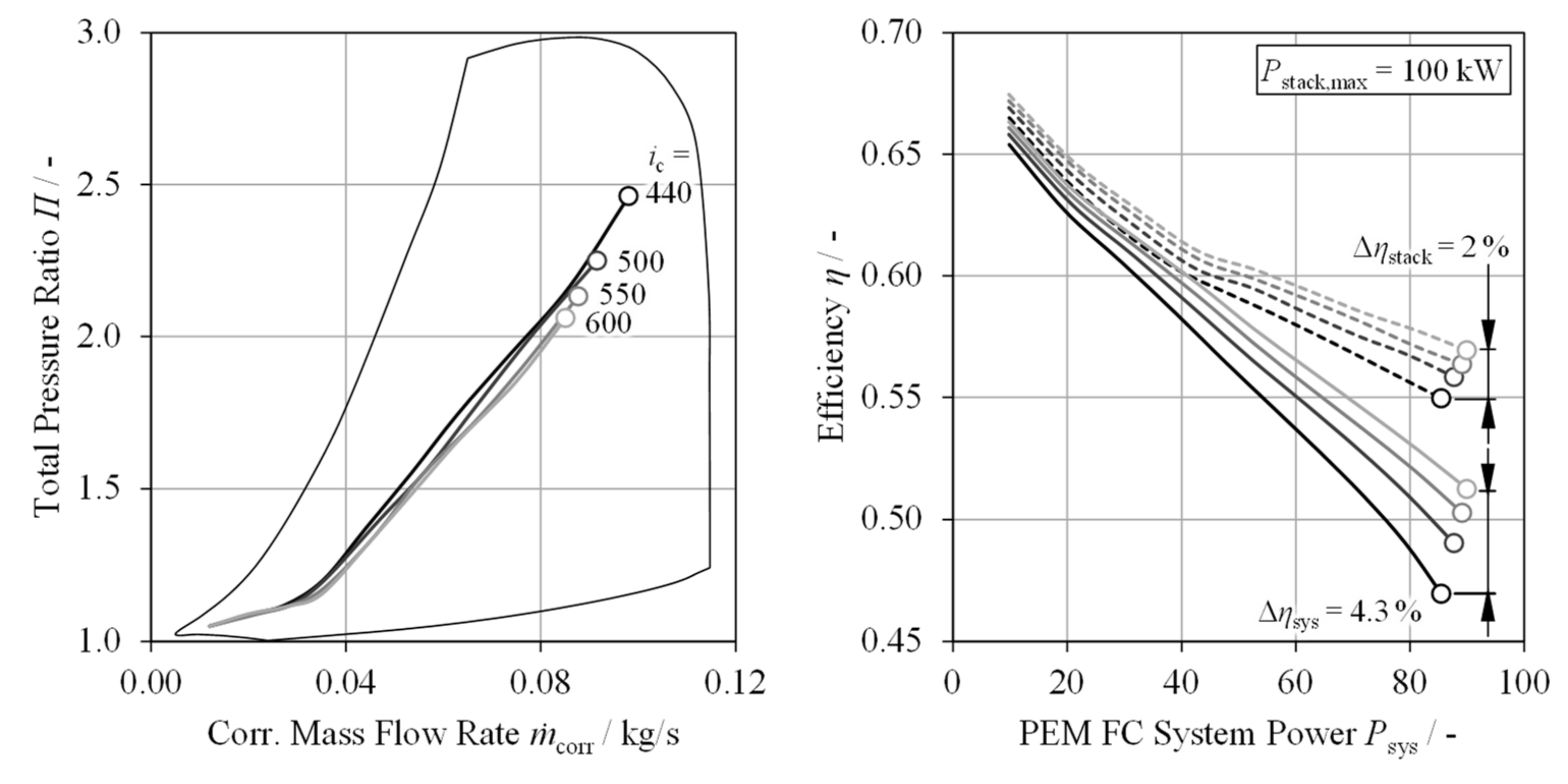
To assess the impact of component sizing on the optimum operating line and the associated PEM FC system efficiency, size variations of stack (cell number) and humidifier (membrane surface area) are investigated. The optimum operating lines shown in the subsequent figures are found analogous to Figure 6 by maximizing system efficiency for all relevant stack power levels.

Starting from the base value of i_c = 440 cells (assumed for Figure 6), stack size is increased to i_c = 600 cells. The associated optimum operating lines and the corresponding stack and system efficiencies are shown in Figure 7.

The stoichiometric oxygen molar flow rate required by the stack ṅ_{O₂,st,stack} is calculated as follows:

$${\dot{n}}_{{\mathrm{O}}_2,\mathrm{s}\mathrm{t},\mathrm{s}\mathrm{t}\mathrm{a}\mathrm{c}\mathrm{k}}=i_{\mathrm{c}}{\displaystyle \frac{I}{4F}}=i_{\mathrm{c}}{\displaystyle \frac{P_{\mathrm{s}\mathrm{t}\mathrm{a}\mathrm{c}\mathrm{k}}}{4F{i}_{\mathrm{c}}U}}\hspace{1em}\to \hspace{1em}{\displaystyle \frac{d{\dot{n}}_{{\mathrm{O}}_2,\mathrm{s}\mathrm{t},\mathrm{s}\mathrm{t}\mathrm{a}\mathrm{c}\mathrm{k}}}{d{i}_{\mathrm{c}}}}<0\hspace{1em}\mathrm{w}\mathrm{i}\mathrm{t}\mathrm{h}\hspace{1em}{\displaystyle \frac{dU}{dI}}<0\hspace{1em},\hspace{1em}{\displaystyle \frac{dI}{d{i}_{\mathrm{c}}}}<0$$

(22)

For increasing i_c, the individual cell operating point is shifted to lower effective current densities and higher cell efficiencies (I ↓ → j_eff ↓ → U ↑), and the required cathode air mass flow rate and the corresponding corrected compressor mass flow rate are reduced. At the same time, the sensitivity dU/dp is reduced for j_eff ↓ (cf. Figure 2), increasing boost pressure levels yield diminishing returns. Consequently, the optimum compressor pressure ratio is reduced.

Overall, the optimum compressor operating points are shifted to lower ṁ_corr and Π. The overall location of the optimum operating line within the compressor map remains approximately constant. Increasing the stack size by 36% (i_c = 440 → 600) yields a stack efficiency gain of Δη_stack = 2% in the rated operating point. Here, compressor power is reduced by 32%, resulting in a system efficiency increase of Δη_sys = 4.3%.

Increasing the stack size is an effective measure to improve PEM FC system efficiency both by increasing stack efficiency as well as by reducing the required compressor power. This is offset by higher system cost and weight. The decision on optimum stack size must therefore always take economic criteria into account (i.e., the total cost of ownership calculation, cf. [37]).

Apart from the cell number, the membrane humidifier size has a significant impact on PEM FC system performance and compressor operating strategy. To assess this impact, a humidifier membrane variation is carried out. Starting from the initial value of A = 3.6 m² (used in Figure 6), the humidifier membrane surface area is scaled (A → A′) according to the following equation:

$$A^{\prime }=f_{\mathrm{b}}A\hspace{1em}\mathrm{w}\mathrm{i}\mathrm{t}\mathrm{h}\hspace{1em}{f}_{\mathrm{b}}=0.25\dots 3$$

(23)

The associated optimum operating lines and the corresponding stack and PEM FC system efficiencies are shown in Figure 8.

For small humidifier membrane surface areas, RH_p,out is insufficient, even in operating points with RH_f,in ≥ 1. The relative humidity levels required for satisfactory PEM conductivity can only be achieved if the operating pressure (Π) is increased. At the same time, cathode stoichiometry (ṁ_corr) must be reduced to lower the amount of reaction product water transported out of the cell.

In contrast, cell humidity levels can become too high for large humidifier membrane surface areas. Here, cathode stoichiometry must be increased to reduce the specific water transfer in the humidifier (cf. Figure 4) and to transport excess product water out of the cell to avoid cell flooding. The operating pressure must be reduced to lower the relative humidity for constant water mass fraction. Overall, ṁ_corr is substituted for Π with f_b ↑. P_el remains approximately constant within the respective operating points, and changes in η_stack are directly translated to η_sys.

For the investigated example, f_b = 1 yields the highest system efficiency at the rated power. For larger humidifier membrane surface areas, cell flooding can be observed above P_sys ≈ 75 kW, resulting in decreased stack and PEM FC system efficiency (cf. detailed view in Figure 8).

3.2. Cell Ageing

Over the course of its useful life, the PEM FC stack experiences various aging effects which negatively impact cell performance (cf. e.g., [38,39,40]). The majority of these effects can be modeled by a decrease in active cell area.

In [41], the United States Department of Energy (US DoE) defines two different end-of-life criteria for PEM FC systems:

• A 10% reduction of the maximum stack power compared to the new system;
• A 5% reduction of the cell voltage at the nominal current density j_nom = 1.2 A/cm² compared to the new system.

To assess the first criterion, the rated power operating point derived in Figure 6 is considered. The active cell area is scaled (A_z → A′_z) according to

$$A_{\mathrm{z}}^{\prime }=f_{\mathrm{A}}{A}_{\mathrm{z}}\hspace{1em}\mathrm{w}\mathrm{i}\mathrm{t}\mathrm{h}\hspace{1em}{f}_{\mathrm{A}}<1$$

(24)

while ṁ_corr = 0.102 kg/s and Π = 2.41 are kept constant. Under these boundary conditions, the new system can reach a maximum stack power of P_stack,lim = 112 kW. As shown in Figure 9, f_A = 0.813 yields a 10% reduction of P_stack,lim (ṁ_corr, Π = const.)

For the second criterion, the nominal current density j_nom is introduced. j_nom relates the cell current to the geometric cell area (equivalent to the active cell area in new condition) whereas j_eff references the actual active cell area.

$$j_{\mathrm{e}\mathrm{f}\mathrm{f}}={\displaystyle \frac{I}{A_z^{\prime }}}=\mathrm{c}\mathrm{o}\mathrm{n}\mathrm{s}\mathrm{t}.\hspace{1em}\to \hspace{1em}{j}_{\mathrm{n}\mathrm{o}\mathrm{m}}={\displaystyle \frac{I}{A_{\mathrm{z}}}}\propto {\displaystyle \frac{1}{f_{\mathrm{A}}}}$$

(25)

j_nom = 1.2 A/cm² is reached at P_stack = 90 kW with the optimum operating strategy determined in Figure 6. Keeping the corresponding operating boundary conditions constant (ṁ_corr = 0.085 kg/s, Π = 2.17), f_A = 0.812 yields a 5% reduction of U (j_nom = 1.2 A/cm²).

Aging effects can be compensated for if the cathode stoichiometry and operating pressure are increased. Figure 9 shows the minimum ṁ_corr, Π parameter combination required to reach stack rated power P_stack,lim = 100 kW in dependence of f_A.

As explained for Figure 6, a limit curve Π_min = f (ṁ_corr) exists for each stack target power P_stack,target, below which P_stack,lim < P_stack,target occurs. As Figure 9 shows, this limit curve is shifted to higher ṁ_corr and Π for f_A ↓ (A_z ↓ → j_eff ↑ → sensitivity for λ_c, p ↑).

A decreasing stack performance (f_A ↓) must be compensated for by increasing ṁ_corr and Π (while accepting system efficiency losses). Any compressor operating point above the limit curve Π_min = f (ṁ_corr, f_A) is suitable for this purpose. However, analogous to Figure 6, it is preferred to select the compressor operating point which maximizes η_sys.

For f_A = 0.8, this yields the rated operating point highlighted in Figure 9 (ṁ_max, Π_max). If the PEM FC system shall provide constant rated power until the end of its service life, the rated operating point must lie within the compressor map limits and the electric machine must provide the compressor drive power required to reach the rated operating point (cf. Section 4.2).

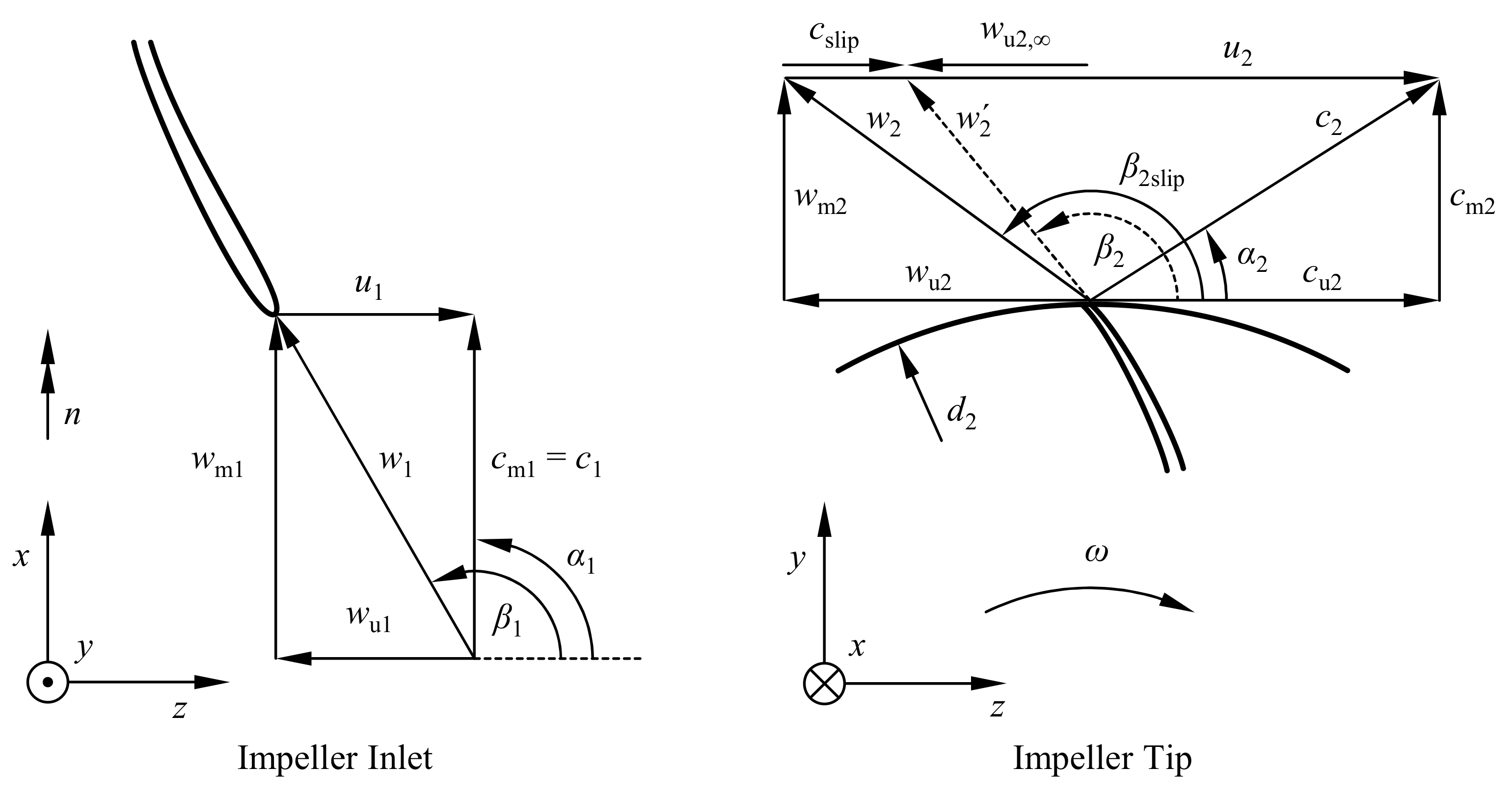
4. Compressor Preliminary Design

The centrifugal compressor preliminary design process is centered around the machine design flow parameter φ_M,des. φ_M,des relates design mass flow rate ṁ_des, design speed n_des, impeller tip diameter d₂ and compressor inlet conditions (stage inlet total density ρ_t0) [3,42]:

$${\phi }_{\mathrm{M},\mathrm{d}\mathrm{e}\mathrm{s}}={\displaystyle \frac{4{\dot{m}}_{\mathrm{d}\mathrm{e}\mathrm{s}}}{{\rho }_{\mathrm{t}0}{d}_2^3{\pi }^2{n}_{\mathrm{d}\mathrm{e}\mathrm{s}}}}$$

(26)

The compressor design mass flow rate ṁ_des = 0.102 kg/s and design pressure ratio Π_des = 2.41 have been determined within system simulation (cf. Figure 6). For these values, the design point compressor power P_c,des can be calculated as follows [3]:

$$P_{\mathrm{c},\mathrm{d}\mathrm{e}\mathrm{s}}={\displaystyle \frac{1}{{\eta }_{\mathrm{s}}}}{\dot{m}}_{\mathrm{d}\mathrm{e}\mathrm{s}}{c}_{\mathrm{p}}{T}_{\mathrm{t}0}\left({\Pi }_{\mathrm{d}\mathrm{e}\mathrm{s}}^{{\displaystyle \frac{\kappa -1}{\kappa }}}-1\right)={\dot{m}}_{\mathrm{d}\mathrm{e}\mathrm{s}}{\lambda }_{\mathrm{h}}{u}_{2,\mathrm{d}\mathrm{e}\mathrm{s}}^2$$

(27)

T_t0 denotes the total temperature at the compressor stage inlet, c_p is the working fluid´s heat capacity at a constant pressure and κ is the isentropic exponent.

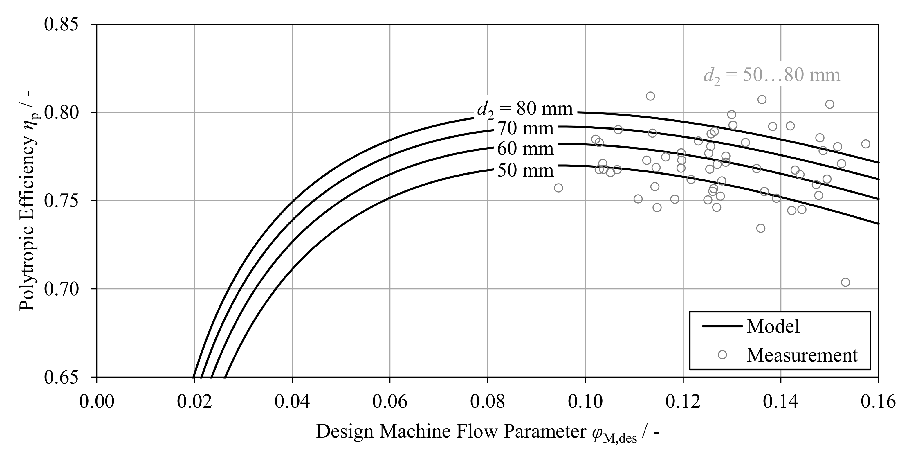
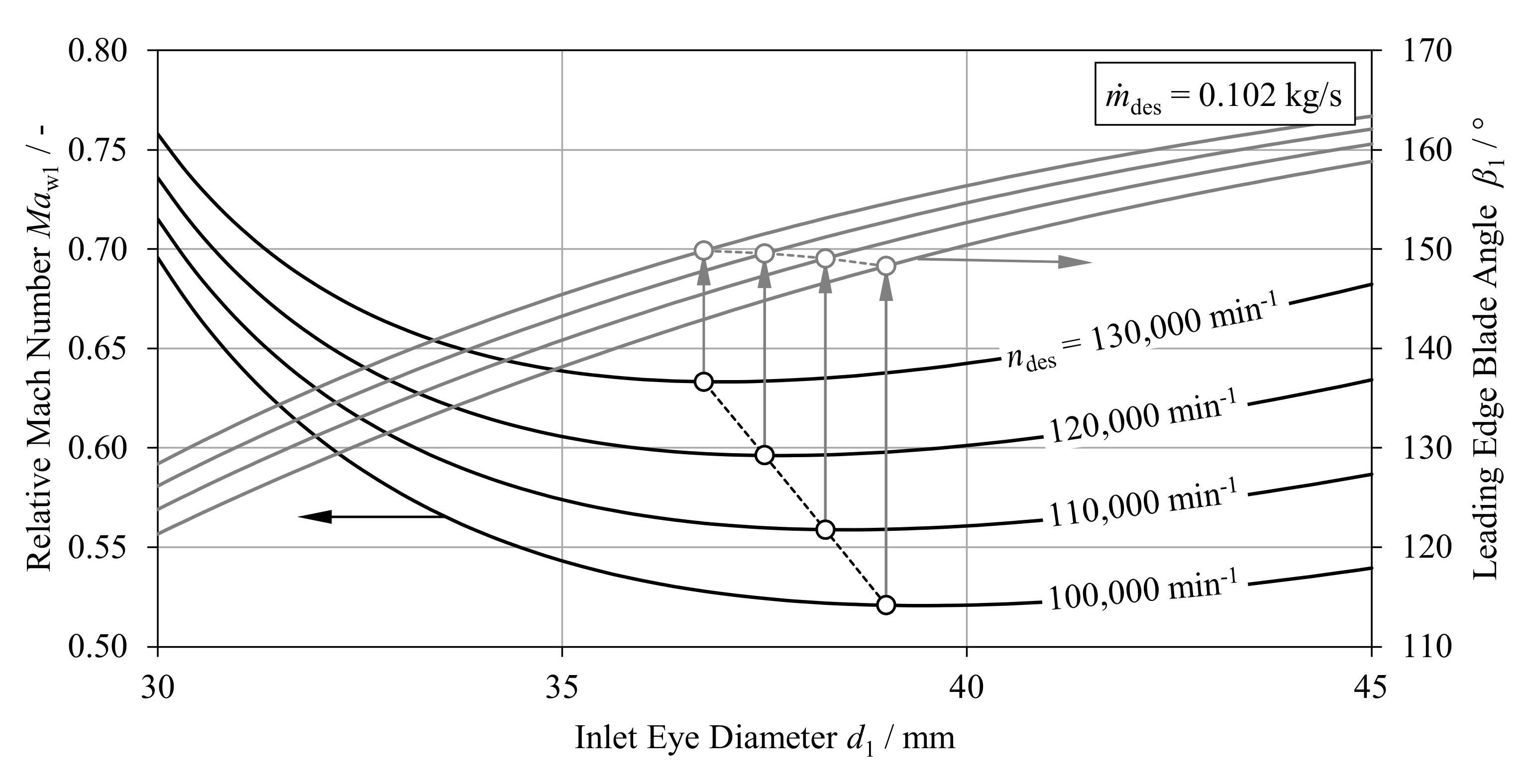
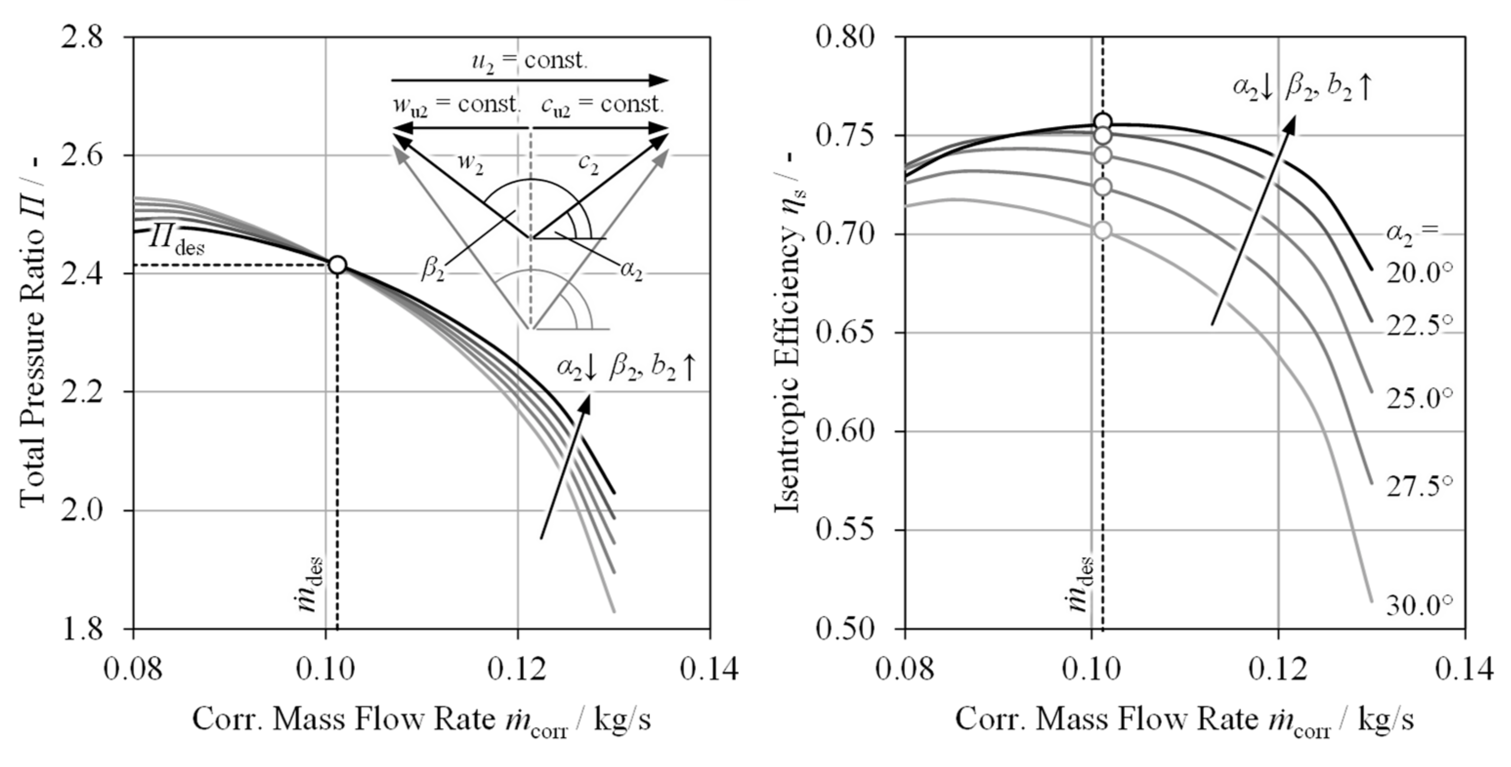
4.1. Compressor Stage Sizing

Introducing the circumferential design speed u_2,des, Equation (26) can be reformulated to yield the impeller tip diameter d₂:

$$d_2^3={\displaystyle \frac{4{\dot{m}}_{\mathrm{d}\mathrm{e}\mathrm{s}}}{{\rho }_{\mathrm{t}0}{\pi }^2{\phi }_{\mathrm{M},\mathrm{d}\mathrm{e}\mathrm{s}}{n}_{\mathrm{d}\mathrm{e}\mathrm{s}}}}\hspace{1em},\hspace{1em}{n}_{des}={\displaystyle \frac{u_{2,\mathrm{d}\mathrm{e}\mathrm{s}}}{d_2\pi }}\hspace{1em}\to \hspace{1em}{d}_2=\sqrt{{\displaystyle \frac{4{\dot{m}}_{\mathrm{d}\mathrm{e}\mathrm{s}}}{{\rho }_{\mathrm{t}0}\pi {\phi }_{\mathrm{M},\mathrm{d}\mathrm{e}\mathrm{s}}{u}_{2,\mathrm{d}\mathrm{e}\mathrm{s}}}}}$$

(28)

To solve Equation (27) or Equation (28), estimates for the isentropic compressor efficiency η_s and work input coefficient λ_h must be found. η_s is derived from the polytropic compressor efficiency η_p in dependence of the pressure ratio Π [18]:

$${\eta }_{\mathrm{s}}={\displaystyle \frac{{\Pi }^{\frac{\kappa -1}{\kappa }}-1}{{\Pi }^{\frac{\kappa -1}{{\eta }_{\mathrm{p}}\kappa }}-1}}$$

(29)

Based on the work of [8] and evaluations of automotive exhaust gas turbocharger performance data, the following empirical relation for the polytropic compressor efficiency is introduced:

$${\eta }_{\mathrm{p}}=1-\left[{\left({\displaystyle \frac{175 \mathrm{m}\mathrm{m}}{d_2}}\right)}^{0.35}\left(1-{\eta }_{\mathrm{p},\mathrm{r}\mathrm{e}\mathrm{f}}\right)\right]$$

(30)

For the reference polytropic compressor efficiency η_p,ref, the relation suggested in [42] is used:

$$\begin{array}{c}{\eta }_{\mathrm{p},\mathrm{r}\mathrm{e}\mathrm{f}}={\eta }_{\mathrm{p},0}-{\displaystyle \frac{0.017}{0.04+5{\phi }_{\mathrm{M},\mathrm{d}\mathrm{e}\mathrm{s}}+{\eta }_{\mathrm{p},0}}}\\ \mathrm{w}\mathrm{i}\mathrm{t}\mathrm{h}\hspace{1em}{\eta }_{\mathrm{p},0}={\displaystyle \frac{1}{{\lambda }_{\mathrm{h}}}}\left(0.59+0.7{\phi }_{\mathrm{M},\mathrm{d}\mathrm{e}\mathrm{s}}-7.5{\phi }_{\mathrm{M},\mathrm{d}\mathrm{e}\mathrm{s}}-{\displaystyle \frac{0.00025}{{\phi }_{\mathrm{M},\mathrm{d}\mathrm{e}\mathrm{s}}}}\right)\end{array}$$

(31)

Figure 10 shows Equation (30) for varying design machine flow parameters and impeller tip diameters.

Ref. [42] also provides an estimate for the work input coefficient λ_h:

$${\lambda }_{\mathrm{h}}=0.68-{\left({\displaystyle \frac{{\phi }_{\mathrm{M},\mathrm{d}\mathrm{e}\mathrm{s}}}{0.37}}\right)}^3+{\displaystyle \frac{0.002}{{\phi }_{\mathrm{M},\mathrm{d}\mathrm{e}\mathrm{s}}}}$$

(32)

With Equation (32), the design isentropic work input coefficient λ_y,des follows:

$${\lambda }_{\mathrm{y},\mathrm{d}\mathrm{e}\mathrm{s}}={\displaystyle \frac{y_{\mathrm{d}\mathrm{e}\mathrm{s}}}{u_{2,\mathrm{d}\mathrm{e}\mathrm{s}}^2}}={\eta }_{\mathrm{s}}{\lambda }_{\mathrm{h}}\hspace{1em}\mathrm{w}\mathrm{i}\mathrm{t}\mathrm{h}\hspace{1em}{y}_{\mathrm{d}\mathrm{e}\mathrm{s}}=c_{\mathrm{p}}{T}_{\mathrm{t}0}\left({\Pi }_{\mathrm{d}\mathrm{e}\mathrm{s}}^{{\displaystyle \frac{\kappa -1}{\kappa }}}-1\right)$$

(33)

y_des denotes the specific isentropic compressor work at design point operation. u_2,des can subsequently be expressed as follows:

$$u_{2,\mathrm{d}\mathrm{e}\mathrm{s}}=\sqrt{{\displaystyle \frac{c_{\mathrm{p}}{T}_{\mathrm{t}0}\left({\mathsf{\Pi }}_{\mathrm{d}\mathrm{e}\mathrm{s}}^{\frac{\kappa -1}{\kappa }}-1\right)}{{\lambda }_{\mathrm{y},\mathrm{d}\mathrm{e}\mathrm{s}}}}}$$

(34)

This yields the impeller tip diameter d₂ and the design speed n_des, as follows:

$$d_2=2\sqrt{{\displaystyle \frac{{\dot{m}}_{\mathrm{d}\mathrm{e}\mathrm{s}}}{{\rho }_{\mathrm{t}0}\pi u_{2,\mathrm{d}\mathrm{e}\mathrm{s}}{\phi }_{\mathrm{M},\mathrm{d}\mathrm{e}\mathrm{s}}}}}\hspace{1em},\hspace{1em}{n}_{\mathrm{d}\mathrm{e}\mathrm{s}}={\displaystyle \frac{u_{2,\mathrm{d}\mathrm{e}\mathrm{s}}}{d_2\pi }}$$

(35)

Using this set of equations, d₂ and n_des can be estimated for a given design point (ṁ_des, Π_des) at a specified design flow parameter φ_M,des.

At this point, the main compressor design parameters are defined. The next preliminary design step includes the selection of blade angles β and blade heights b at the impeller inlet (index ₁) and the impeller tip (index ₂). Figure 11 shows the meridional (Index _m) and circumferential (Index _u) flow velocities in the inertial and moving reference frame (absolute velocities c and relative velocities w).

The impeller inlet blade angle β₁ (evaluated at the blade tip) is selected to yield an incidence-free leading-edge flow in the design point (flow angle matches blade angle). The inlet eye diameter d₁ is then selected to minimize the relative flow velocity w₁ (and associated losses). To achieve this, the following must hold (assuming swirl-free inlet eye flow, c_u1 = 0):

$$c_{\mathrm{m}1}=w_{\mathrm{m}1}={\displaystyle \frac{4{\dot{m}}_{\mathrm{d}\mathrm{e}\mathrm{s}}}{{\rho }_1{d}_1^2\pi }}\hspace{1em},\hspace{1em}{w}_{\mathrm{u}1}=-u_1=d_1\pi n_{\mathrm{d}\mathrm{e}\mathrm{s}} \to \hspace{1em}{\beta }_1=\arctan \left({\displaystyle \frac{w_{\mathrm{m}1}}{w_{\mathrm{u}1}}}\right)+\pi$$

(36)

Figure 12 shows the relative impeller inlet Mach number Ma_w1 and corresponding inlet blade angle β₁ as functions of the inlet eye diameter d₁ for the exemplary design mass flow rate. The impeller inlet density ρ₁ is calculated from stagnation conditions at the stage inlet assuming isentropic flow in the inlet cone.

Increasing n_des requires a reduction of d₁. β₁ is only marginally affected by n_des and remains around β_1,opt ≈ 150°. This is in line with the recommendations given in [42,43].

The impeller tip geometry is selected to achieve target blade work input in the design point. Pressure losses are minimized while maintaining a sufficiently large surge margin.

For swirl-free inlet conditions (c_u1 = 0), the Euler work coefficient λ_EULER is given by the following equation:

$${\lambda }_{\mathrm{E}\mathrm{U}\mathrm{L}\mathrm{E}\mathrm{R}}={\displaystyle \frac{c_{\mathrm{u}2}}{u_2}}={\lambda }_{\mathrm{h}}-{\lambda }_{\mathrm{p}\mathrm{a}\mathrm{r}}\hspace{1em}\mathrm{w}\mathrm{i}\mathrm{t}\mathrm{h}\hspace{1em}{\lambda }_{\mathrm{p}\mathrm{a}\mathrm{r}}={\displaystyle \frac{0.002\dots 0.004}{{\phi }_{\mathrm{M},\mathrm{d}\mathrm{e}\mathrm{s}}}}$$

(37)

The parasitic work input coefficient λ_par is estimated according to [42,44]. λ_par accounts for impeller work that does not contribute to tangential flow acceleration (i.e., tip gap loss, recirculation work and disk friction, cf. [42]). Absolute tangential velocity c_u2 can be written as follows:

$$c_{\mathrm{u}2}=w_{\mathrm{u}2}+u_2={\lambda }_{\mathrm{E}\mathrm{U}\mathrm{L}\mathrm{E}\mathrm{R}}{u}_2$$

(38)

As φ_M,des and u₂ are considered constant for a given preliminary design candidate (cf. Equations (26) and (28)), the following holds:

$${\lambda }_{\mathrm{h}},{\lambda }_{\mathrm{p}\mathrm{a}\mathrm{r}}=f\left({\phi }_{\mathrm{M},\mathrm{d}\mathrm{e}\mathrm{s}}\right)=\mathrm{c}\mathrm{o}\mathrm{n}\mathrm{s}\mathrm{t}. \to \hspace{1em}{\lambda }_{\mathrm{E}\mathrm{U}\mathrm{L}\mathrm{E}\mathrm{R}}=\mathrm{c}\mathrm{o}\mathrm{n}\mathrm{s}\mathrm{t}. \to \hspace{1em}{c}_{\mathrm{u}2}=\mathrm{c}\mathrm{o}\mathrm{n}\mathrm{s}\mathrm{t}.$$

(39)

The remaining velocity components can subsequently be written as follows:

$$c_{\mathrm{m}2}=c_{\mathrm{u}2}\tan \left({\alpha }_2\right)\hspace{1em},\hspace{1em}{c}_2=\sqrt{c_{\mathrm{m}2}^2+c_{\mathrm{u}2}^2}\hspace{1em},\hspace{1em}{w}_2=\sqrt{c_{\mathrm{m}2}^2+w_{\mathrm{u}2}^2}$$

(40)

α₂ is the design flow angle in the inertial reference system.

Due to three-dimensional blade passage flow, the relative flow angle does not follow the tip blade angle for finite blade numbers (cf. [42,45,46]). The slip velocity c_slip describes the tangential velocity difference between the (theoretical) case of the infinite blade number w_u2,∞ (perfect flow guidance) and the actual relative tangential velocity w_u2. c_slip is estimated using the empirical relation for the slip factor σ_WIESNER defined in [45]:

$$\begin{array}{c}{c}_{\mathrm{s}\mathrm{l}\mathrm{i}\mathrm{p}}=w_{\mathrm{u}2,\mathrm{\infty }}-w_{\mathrm{u}2}=\left(1-{\sigma }_{\mathrm{W}\mathrm{I}\mathrm{E}\mathrm{S}\mathrm{N}\mathrm{E}\mathrm{R}}\right)u_2\\ \mathrm{w}\mathrm{i}\mathrm{t}\mathrm{h}\hspace{1em}{\sigma }_{\mathrm{W}\mathrm{I}\mathrm{E}\mathrm{S}\mathrm{N}\mathrm{E}\mathrm{R}}=1-{\displaystyle \frac{\sqrt{\sin \left({\beta }_2\right)}}{z_{\mathrm{e}\mathrm{f}\mathrm{f}}^{0.7}}}\sin \left({\alpha }_{\mathrm{c}2}\right)\hspace{1em},\hspace{1em}{z}_{\mathrm{e}\mathrm{f}\mathrm{f}}=z\left(1-x_{\mathrm{s}\mathrm{p}\mathrm{l}\mathrm{i}\mathrm{t}}\right)\end{array}$$

(41)

z_eff is the effective blade number calculated from the main blade number z and the splitter blade extension ratio x_split. α_c2 is the meridional passage angle at the impeller tip. Evaluating Figure 11, the tip blade angle β₂ is found:

$${\beta }_2=\pi -\arctan \left({\displaystyle \frac{c_{\mathrm{m}2}}{w_{\mathrm{u}2}+c_{\mathrm{s}\mathrm{l}\mathrm{i}\mathrm{p}}}}\right)$$

(42)

The tip blade height b₂ is selected to yield the desired meridional flow velocity c_m2:

$$c_{\mathrm{m}2}={\displaystyle \frac{{\dot{m}}_{\mathrm{d}\mathrm{e}\mathrm{s}}}{{\rho }_2{b}_2{d}_2\pi \left(1-B_2\right)}}=c_{\mathrm{u}2}\tan \left({\alpha }_2\right);\hspace{1em}\mathrm{as}\mathrm{in}\mathrm{E}\mathrm{q}\mathrm{u}\mathrm{a}\mathrm{t}\mathrm{i}\mathrm{o}\mathrm{n} (40)$$

(43)

The blade passage blockage factor B₂ accounts for uneven flow velocity around the circumference and along the blade passage height. B₂ is estimated according to [42].

To determine the thermodynamic impeller tip state (i.e., ρ₂ = p₂/(R_m T₂)), the impeller isentropic efficiency η_s,12 is required. For this purpose, the estimate provided in [42] is corrected for impeller size analogous to Equation (30). The specific isentropic impeller work y₁₂ is calculated according to the following equation:

$$\begin{array}{c}{y}_{12}={\eta }_{\mathrm{s},12}{\lambda }_{\mathrm{E}\mathrm{U}\mathrm{L}\mathrm{E}\mathrm{R}}{u}_2^2=c_{\mathrm{p}}{T}_{\mathrm{t}1}\left({{\displaystyle \frac{p_{\mathrm{t}2}}{p_{\mathrm{t}1}}}}^{{\displaystyle \frac{\kappa -1}{\kappa }}}-1\right)\\ \mathrm{w}\mathrm{i}\mathrm{t}\mathrm{h} {\eta }_{\mathrm{s},12}=1-{\left({\displaystyle \frac{175 \mathrm{m}\mathrm{m}}{d_2}}\right)}^{0.35}\left(1-{\eta }_{\mathrm{s},12,\mathrm{r}\mathrm{e}\mathrm{f}}\right)\\ {\eta }_{\mathrm{s},12,\mathrm{r}\mathrm{e}\mathrm{f}}=f\left({\eta }_{\mathrm{p},12,\mathrm{r}\mathrm{e}\mathrm{f}}, {\displaystyle \frac{p_{\mathrm{t}2}}{p_{\mathrm{t}1}}}\right) [\mathrm{E}\mathrm{q}\mathrm{u}\mathrm{a}\mathrm{t}\mathrm{i}\mathrm{o}\mathrm{n} \left(29\right)]\hspace{1em},\hspace{1em}{\eta }_{\mathrm{p},12,\mathrm{r}\mathrm{e}\mathrm{f}}=0.95-{\displaystyle \frac{0.0005}{{\phi }_{\mathrm{M},\mathrm{d}\mathrm{e}\mathrm{s}}}} [42]\end{array}$$

(44)

Equation (32) (for T_t2), Equation (44) (for p_t2) and Equation (43) (for c₂, T₂ and p₂) are iteratively solved to determine ρ₂.

The impeller tip geometry can now be fully defined in dependence of α₂. Figure 13 shows exemplary design speed lines for varying α₂.

The tip flow coefficient φ₂ relates the meridional tip velocity c_m2 to the circumferential speed u₂. In the design point its derivative is given as follows:

$${\phi }_2={\displaystyle \frac{c_{\mathrm{m}2}}{u_2}} \to \hspace{1em}{{\displaystyle \frac{d{\phi }_2}{d\dot{m}}}}_{|\mathrm{d}\mathrm{e}\mathrm{s}}=\underset{=\mathrm{c}\mathrm{o}\mathrm{n}\mathrm{s}\mathrm{t}.}{\underbrace{{\displaystyle \frac{1}{u_{2,\mathrm{d}\mathrm{e}\mathrm{s}}{d}_2\left(1-B_2\right)}}}}{\displaystyle \frac{1}{{\rho }_2{b}_2}}$$

(45)

η_s = f(φ_M,des) = const. yields λ_y ∝ λ_h. With λ_par = const., the total pressure ratio derivative dΠ^/dṁ can be estimated based on the derivative dλ_EULER^/dṁ:

$$\begin{array}{c}{\lambda }_{\mathrm{E}\mathrm{U}\mathrm{L}\mathrm{E}\mathrm{R}}={\displaystyle \frac{c_{u2}}{u_2}}={\sigma }_{\mathrm{W}\mathrm{I}\mathrm{E}\mathrm{S}\mathrm{N}\mathrm{E}\mathrm{R}}+{\displaystyle \frac{{\phi }_2}{\tan \left({\beta }_2\right)}}\\ {{\displaystyle \frac{d{\lambda }_{\mathrm{E}\mathrm{U}\mathrm{L}\mathrm{E}\mathrm{R}}}{d\dot{m}}}}_{|\mathrm{d}\mathrm{e}\mathrm{s}}=\underset{={\displaystyle \frac{1}{\tan \left({\beta }_2\right)}}}{\underbrace{{\displaystyle \frac{d{\lambda }_{\mathrm{E}\mathrm{U}\mathrm{L}\mathrm{E}\mathrm{R}}}{d{\phi }_2}}}}{{\displaystyle \frac{d{\phi }_2}{d\dot{m}}}}_{|\mathrm{d}\mathrm{e}\mathrm{s}}\propto \left(-1\right)\underset{\begin{array}{c}\left(1\right)\\ \uparrow \mathrm{f}\mathrm{o}\mathrm{r} {\beta }_2\uparrow \end{array}}{\underbrace{{\displaystyle \frac{1}{\left|\tan \left({\beta }_2\right)\right|}}} }\underset{\begin{array}{c}\left(2\right)\\ \downarrow \mathrm{f}\mathrm{o}\mathrm{r} {\beta }_2\uparrow \end{array}}{\underbrace{ {\displaystyle \frac{1}{{\rho }_2{b}_2}}} }\end{array}$$

(46)

β₂ ↑ (α₂ ↓) results in a higher (negative) gradient of the λ_EULER, φ₂ line (term 1 in Equation (46)). At the same time, the influence of dṁ on dφ₂ is reduced for b₂ ↑ (term 2 in Equation (46)). The latter dominant effect is magnified due to ρ₂ ↑ (ρ₂ ↑ with c₂ ↓ for p_t2, T_t2, ρ_t2 ≈ const.). The sum of both effects results in a decreasing absolute speed line gradient for β₂ ↑.

For α₂ ↑, c_m2 must be increased to keep c_u2 = const. (cf. Figure 11). w₂ and c₂ increase accordingly, resulting in higher impeller and diffuser losses. From an efficiency standpoint, α₂ should therefore be minimized. Low α₂, however, may result in diffuser stall:

$${\alpha }_{2,\mathrm{m}\mathrm{i}\mathrm{n}}=0.24\left[1-\exp \left(-36.4{\displaystyle \frac{b_2}{d_2}}\right)\right]$$

(47)

α_2,min is the minimum stall-free diffuser inlet flow angle. Equation (47) is derived graphically from the relations given in [42,47].

Based on φ_M,des, ref. [42] suggests a design impeller tip flow angle α_2,des to assure a sufficient surge margin relative to the design point. Transient PEM FC system simulations show that the deviation from the stationary operating line derived in Figure 6 remains small, even for high stack power gradients (using a suitable control strategy, cf. [11]). Against this background, the required surge margin and α_2,des can be reduced below the value recommended in [42]:

$${\alpha }_{2,\mathrm{d}\mathrm{e}\mathrm{s}}=\arctan \left(a+3{\phi }_{\mathrm{M},\mathrm{d}\mathrm{e}\mathrm{s}}\right)\hspace{1em}\mathrm{w}\mathrm{i}\mathrm{t}\mathrm{h}\hspace{1em}a=\left\{\begin{array}{cc}0.26& \mathrm{i}\mathrm{n} [42]\\ 0.20& \mathrm{h}\mathrm{e}\mathrm{r}\mathrm{e}\end{array}\right.$$

(48)

Diffuser performance is estimated using the one-dimensional model described in [48]. To reduce the parameter set size in the preliminary design step, a parallel-walled diffuser is used. A diffuser diameter ratio (outlet to inlet) around x_diff = d₄^/d₂ ≈ 1.75 is found to provide good efficiency for the considered design tip flow angles.

The volute cross section is selected to conserve angular momentum by complying to the well-known sizing rules presented in [8,42,49]:

$$r_{\mathrm{v}\mathrm{o}\mathrm{l}}{c}_{\mathrm{m}}=r_4{c}_{\mathrm{u}4}\hspace{1em}\mathrm{w}\mathrm{i}\mathrm{t}\mathrm{h}\hspace{1em}{r}_4={\displaystyle \frac{d_4}{2}}\hspace{1em},\hspace{1em}\rho c_{\mathrm{m}}{A}_{\mathrm{v}\mathrm{o}\mathrm{l}}={\rho }_4{d}_4{b}_4{c}_{\mathrm{m}4}\theta$$

(49)

r_vol is the radial coordinate of the volute cross section´s center of gravity. Index ₄ marks the diffuser outlet. Re-arranging Equation (49) yields A_vol in dependence of the design flow angle at the diffuser outlet α_4,des and the angular coordinate θ:

$$A_{\mathrm{v}\mathrm{o}\mathrm{l}}=\theta r_{\mathrm{v}\mathrm{o}\mathrm{l}}{b}_4{{\displaystyle \frac{c_{\mathrm{m}4}}{c_{\mathrm{u}4}}}}_{|\mathrm{d}\mathrm{e}\mathrm{s}} \to \hspace{1em}{\displaystyle \frac{A_{\mathrm{v}\mathrm{o}\mathrm{l}}}{r_{\mathrm{v}\mathrm{o}\mathrm{l}}}}=\theta b_4\tan \left({\alpha }_{4,\mathrm{d}\mathrm{e}\mathrm{s}}\right)$$

(50)

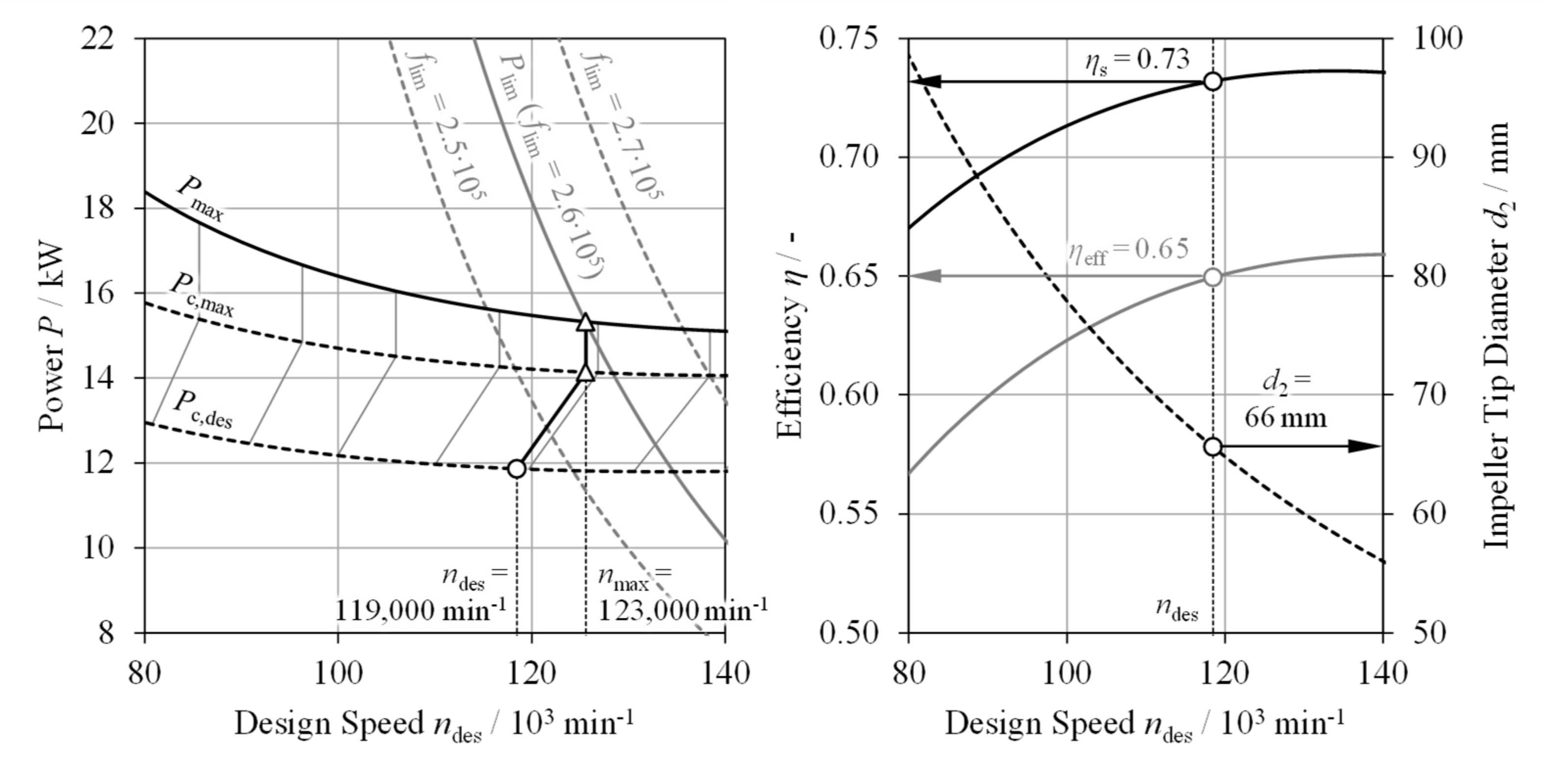
4.2. Electric Machine and Air Bearing Sizing

As described in Section 3.2, PEM FC stack efficiency decreases over the course of the operating life. If the nominal stack power shall be kept constant, the operating pressure and/or cathode stoichiometry must be increased. When designing the electric machine and air bearing system, a power reserve f_res must be considered. f_res links the design pressure ratio used for preliminary compressor sizing (index _des) to the rated operating point pressure ratio of the aged PEM FC system (index _max):

$${\Pi }_{\mathrm{m}\mathrm{a}\mathrm{x}}={\Pi }_{\mathrm{d}\mathrm{e}\mathrm{s}}\left(1+f_{\mathrm{r}\mathrm{e}\mathrm{s}}\right)$$

(51)

Aging simulations show that the machine flow parameter can be considered constant between the design point and the rated operating point (cf. Figure 9). For sufficiently small f_res, constant isentropic efficiency can be assumed, leading to the following:

$${\phi }_{\mathrm{M},\mathrm{d}\mathrm{e}\mathrm{s}}={\phi }_{\mathrm{M},\mathrm{m}\mathrm{a}\mathrm{x}}\hspace{1em},\hspace{1em}{\eta }_{\mathrm{s},\mathrm{d}\mathrm{e}\mathrm{s}}={\eta }_{\mathrm{s},\mathrm{m}\mathrm{a}\mathrm{x}} \to \hspace{1em}{\lambda }_{\mathrm{h},\mathrm{d}\mathrm{e}\mathrm{s}}={\lambda }_{\mathrm{h},\mathrm{m}\mathrm{a}\mathrm{x}}\hspace{1em},\hspace{1em}{\lambda }_{\mathrm{y},\mathrm{d}\mathrm{e}\mathrm{s}}={\lambda }_{\mathrm{y},\mathrm{m}\mathrm{a}\mathrm{x}}$$

(52)

Compressor rated speed n_max, mass flow rate ṁ_max, and power P_c,max can now be calculated:

$$\begin{array}{c}{\displaystyle \frac{y_{\mathrm{m}\mathrm{a}\mathrm{x}}}{u_{2,\mathrm{m}\mathrm{a}\mathrm{x}}^2}}={\displaystyle \frac{y_{\mathrm{d}\mathrm{e}\mathrm{s}}}{u_{2,\mathrm{d}\mathrm{e}\mathrm{s}}^2}} \to \hspace{1em}{u}_{2,\mathrm{m}\mathrm{a}\mathrm{x}}=u_{2,\mathrm{d}\mathrm{e}\mathrm{s}}\sqrt{{\left({\displaystyle \frac{{\Pi }_{\mathrm{m}\mathrm{a}\mathrm{x}}}{{\Pi }_{\mathrm{d}\mathrm{e}\mathrm{s}}}}\right)}^{{\displaystyle \frac{\kappa }{\kappa -1}}}} \to \hspace{1em}{n}_{\mathrm{m}\mathrm{a}\mathrm{x}}={\displaystyle \frac{u_{2,\mathrm{m}\mathrm{a}\mathrm{x}}}{\pi d_2}}\\ {\dot{m}}_{\mathrm{m}\mathrm{a}\mathrm{x}}={\dot{m}}_{\mathrm{d}\mathrm{e}\mathrm{s}}{\displaystyle \frac{u_{2,\mathrm{m}\mathrm{a}\mathrm{x}}}{u_{2,\mathrm{d}\mathrm{e}\mathrm{s}}}}\hspace{1em},\hspace{1em}{P}_{\mathrm{c},\mathrm{m}\mathrm{a}\mathrm{x}}={\dot{m}}_{\mathrm{m}\mathrm{a}\mathrm{x}}{c}_{\mathrm{p}}{T}_{\mathrm{t}0}{\displaystyle \frac{y_{\mathrm{m}\mathrm{a}\mathrm{x}}}{{\eta }_{\mathrm{s},\mathrm{d}\mathrm{e}\mathrm{s}}}}\end{array}$$

(53)

The electric machine must provide the power P_max to drive the compressor at P_c,max and to overcome bearing friction P_f,max:

$$P_{\mathrm{m}\mathrm{a}\mathrm{x}}=P_{\mathrm{c},\mathrm{m}\mathrm{a}\mathrm{x}}+P_{\mathrm{f},\mathrm{m}\mathrm{a}\mathrm{x}}$$

(54)

Limited by mechanical, thermal and electric boundary conditions, electric machines exhibit a trade-off between the rated power P_max and rated speed n_max. As outlined in previous work (cf. [11,12,14,37,50]), for permanent magnet synchronous machines (PMSM) this trade-off can be written as follows:

$${\displaystyle \frac{P_{\mathrm{m}\mathrm{a}\mathrm{x}}}{\mathrm{k}\mathrm{W}}}\le {\left[{\displaystyle \frac{\left(2.6\pm 0.1\right){10}^5}{\frac{n_{\mathrm{m}\mathrm{a}\mathrm{x}}}{{\mathrm{m}\mathrm{i}\mathrm{n}}^{-1}}}}\right]}^{3.75}$$

(55)

According to [51,52], the maximum PMSM torque M_max can be estimated:

$$M_{\mathrm{m}\mathrm{a}\mathrm{x}}={\displaystyle \frac{1}{2}}{f}_{\mathrm{r}}{\tau }_{\mathrm{m}\mathrm{a}\mathrm{x}}\pi \varsigma d_{\mathrm{r}}^3\hspace{1em}\mathrm{w}\mathrm{i}\mathrm{t}\mathrm{h}\hspace{1em}{f}_{\mathrm{r}}=0.7\hspace{1em},\hspace{1em}{\tau }_{\mathrm{m}\mathrm{a}\mathrm{x}}=3.3{\displaystyle \frac{\mathrm{N}}{\mathrm{c}{\mathrm{m}}^2}}\hspace{1em},\hspace{1em}\varsigma ={\displaystyle \frac{l_{\mathrm{r}}}{d_{\mathrm{r}}}}\le 2$$

(56)

The pole coverage factor f_r accounts for decreasing field strength at the stator ends, and the maximum tangential stress τ_max is estimated based on the literature data provided in [52]. The rotor length-to-diameter ratio ς is limited by rotor dynamics. Due to mechanical and thermal stress, the rotor circumferential speed is usually limited to u_r,max ≈ 200 m/s [53]. Accordingly, the rotor diameter d_r is given by the following equation:

$$d_{\mathrm{r}}=\min \left(\sqrt[3]{{\displaystyle \frac{2M_{\mathrm{m}\mathrm{a}\mathrm{x}}}{f_{\mathrm{r}}{\tau }_{\mathrm{m}\mathrm{a}\mathrm{x}}\pi \varsigma }}} ,{\displaystyle \frac{u_{\mathrm{r},\mathrm{m}\mathrm{a}\mathrm{x}}}{\pi n_{\mathrm{m}\mathrm{a}\mathrm{x}}}}\right)\hspace{1em}\mathrm{w}\mathrm{i}\mathrm{t}\mathrm{h}\hspace{1em}{u}_{\mathrm{r},\mathrm{m}\mathrm{a}\mathrm{x}}=200{\displaystyle \frac{\mathrm{m}}{\mathrm{s}}}$$

(57)

Radial air foil bearings and electric machine rotors are assumed to have equal diameters. The radial bearing width w_r is selected according to the literature guideline value of w_r^/d_r = 1 [13]. The load carrying capacity F_x,max of axial air foil bearings is proportional to the bearing surface area A_x and average circumferential speed $\stackrel{\mathrm{-}}{u}$ [54]:

$$F_{\mathrm{x},\mathrm{m}\mathrm{a}\mathrm{x}}={\mathcal{D}}_{\mathrm{x}}\underset{=A_{\mathrm{x}}}{\underbrace{\overline{d}\pi b}}\underset{={\overline{u}}_{\mathrm{m}\mathrm{a}\mathrm{x}} }{\underbrace{\overline{d} \pi n_{\mathrm{m}\mathrm{a}\mathrm{x}}}}\hspace{1em}\mathrm{w}\mathrm{i}\mathrm{t}\mathrm{h}\hspace{1em}\overline{d}={\displaystyle \frac{d_{\mathrm{a}}+d_{\mathrm{i}}}{2}}\hspace{1em},\hspace{1em}b={\displaystyle \frac{d_{\mathrm{a}}-d_{\mathrm{i}}}{2}}\hspace{1em},\hspace{1em}{\mathcal{D}}_{\mathrm{x}}=1{\displaystyle \frac{\mathrm{k}\mathrm{N}\mathrm{s}}{{\mathrm{m}}^3}}$$

(58)

d_a and d_i are the outer and inner bearing diameters, and the load capacity factor $\mathcal{D}$_x is derived from the literature data to represent current state-of-the-art air foil bearings (cf. [13,54,55,56]).

Among others, refs. [57,58] provide suitable approaches to estimate impeller thrust load based on basic geometry data and the operating point. The bearing friction loss P_f is estimated by assuming laminar flow in the lubrication film while calibrating the film thicknesses of the axial and radial bearings to match experimental data from [30]. The electric machine and air bearing system can now be sized iteratively. Effective compressor efficiency η_eff is calculated according to the following equation:

$${\eta }_{\mathrm{e}\mathrm{f}\mathrm{f}}={\eta }_{\mathrm{s}} {\eta }_{\mathrm{f}} {\eta }_{\mathrm{P}\mathrm{M}\mathrm{S}\mathrm{M}} {\eta }_{\mathrm{V}\mathrm{F}\mathrm{D}}\hspace{1em}\mathrm{w}\mathrm{i}\mathrm{t}\mathrm{h}\hspace{1em}{\eta }_{\mathrm{f}}={\displaystyle \frac{P_{\mathrm{c}}}{P_{\mathrm{c}}+P_{\mathrm{f}}}}$$

(59)

The electric machine efficiency η_PMSM is estimated in dependence of the speed and torque from empirically derived dimensionless performance charts. The inverter efficiency is assumed constant at η_VFD = 0.98.

Figure 14 shows the results of the preliminary compressor design process for the exemplary design point (ṁ_des = 0.102 kg/s, Π_des = 2.41).

Referring to Figure 10, φ_M,des (or the corresponding design speed n_des) should be selected as high as possible to achieve optimum compressor efficiency. Accordingly, the intersection between the electric machine trade-off curve and the compressor maximum power curve is selected to represent the rated operating point at n_max = 123,000 min⁻¹. Evaluating Equation (53), the compressor design speed is found at n_des = 119,000 min⁻¹. The impeller tip diameter is set to d₂ = 66 mm, and the isentropic and effective compressor efficiencies are estimated at η_s = 0.73 and η_eff = 0.65, respectively.

The newly introduced preliminary compressor design process allows the user to quickly generate feasible design candidates with satisfactory performance within the constraints imposed by the electric machine and the air bearing system. By executing the process for varying design pressure ratios and mass flow rates, the selection chart shown in Figure 15 is generated.

The selection chart shows the PMSM scatter band data and the corresponding trade-off line introduced in Equation (55). Coordinate grids for the relevant design flow parameter range φ_M,des = 0.05…0.10 are overlaid. To assess the feasibility of a compressor design, the intersection of the relevant design mass flow rate and pressure ratio lines is found. For design points above the trade-off line, no suitable electric machine can be found to provide the required rated power P_max at the desired rated speed n_max. In these cases, φ_M,des must be reduced to shift the intersection below the trade-off line.

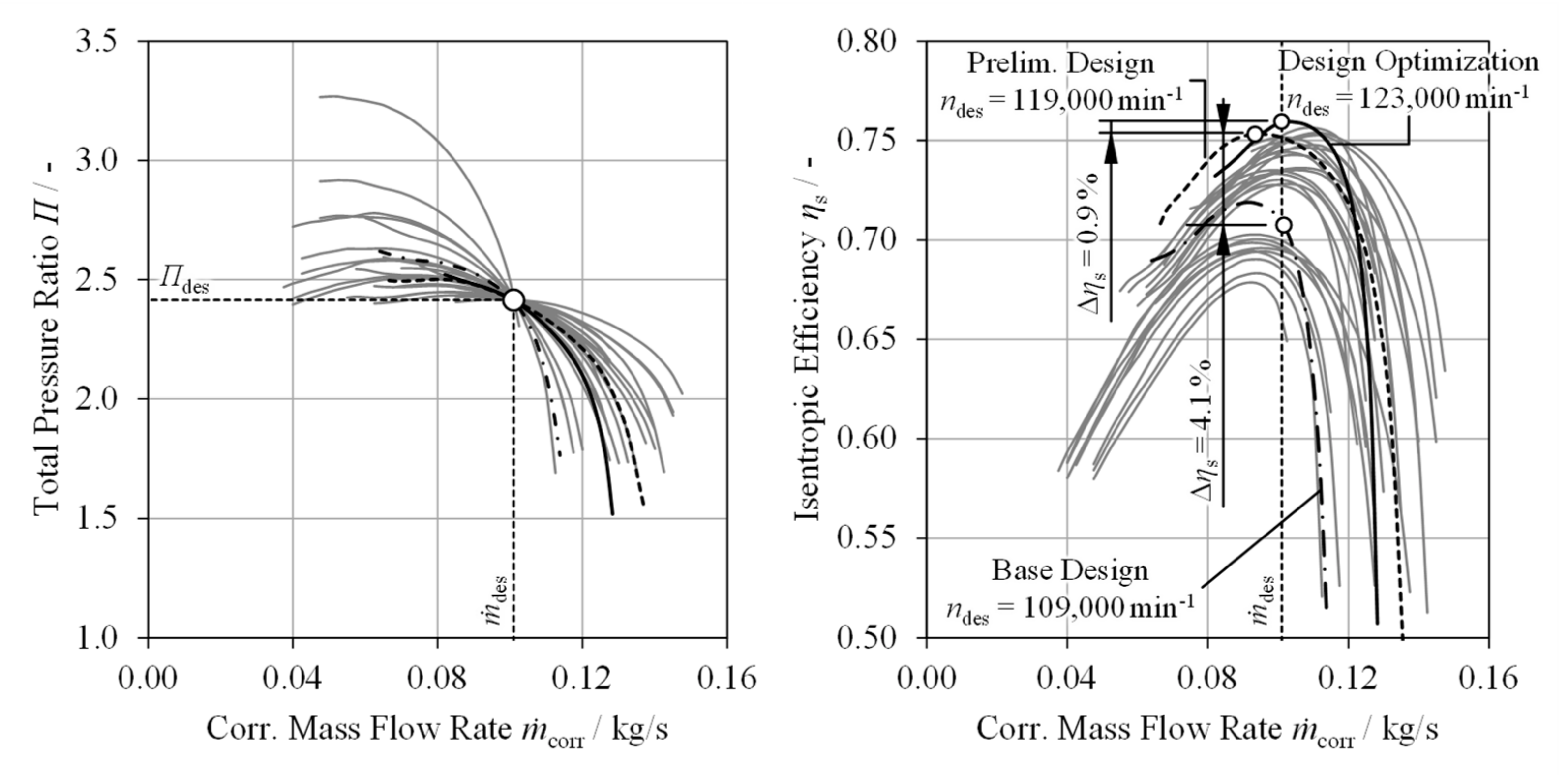
5. Compressor Design Optimization

The preliminary design process provides an initial compressor geometry with satisfactory performance. To further improve design point efficiency, a two-step optimization is performed: A meanline performance model is used to explore a large-scale design space. The design found in this initial optimization step is refined further using three-dimensional computational fluid dynamics simulations (3D CFDs).

The meanline performance model is partially based on the work of [42,48,49]. Adaptions and additions are made to the model to better reflect the operating behavior of low-design machine flow parameter centrifugal compressors. A detailed description of the meanline performance model will be presented in a future publication.

Geometry parameters are varied around the preliminary design (index ₀). Exemplarily, a variation of impeller tip diameter d₂, tip blade angle β₂ and height b₂ as well as diffuser outlet diameter d₄ and height b₄ is performed:

$$\left(\begin{array}{c}\begin{array}{c}{d}_2\\ {\beta }_2\end{array}\\ \begin{array}{c}{b}_2\\ d_4\\ b_4\end{array}\end{array}\right)=\left(\begin{array}{c}\begin{array}{c}{f}_{{\mathrm{d}}_2}\\ f_{{\mathsf{\beta }}_2}\end{array}\\ \begin{array}{c}{f}_{\mathrm{b}}\\ f_{{\mathrm{d}}_4}\\ f_{\mathrm{b}}\end{array}\end{array}\right)\left(\begin{array}{c}\begin{array}{c}{d}_{\mathrm{2,0}}\\ {\beta }_{\mathrm{2,0}}\end{array}\\ \begin{array}{c}{b}_{\mathrm{2,0}}\\ d_{\mathrm{4,0}}\\ b_{\mathrm{4,0}}\end{array}\end{array}\right)\hspace{1em}\mathrm{w}\mathrm{i}\mathrm{t}\mathrm{h}\hspace{1em}\begin{array}{c}\begin{array}{c}{f}_{{\mathrm{d}}_2}=0.8\dots 1.2\\ f_{{\mathsf{\beta }}_2}=0.8\dots 1.2\end{array}\\ \begin{array}{c}{f}_{{\mathrm{d}}_4}=0.7\dots 1.3\\ f_{\mathrm{b}}=0.7\dots 1.3\end{array}\end{array}$$

(60)

In the resulting four-dimensional design space, 6561 parameter combinations are evaluated. Among those, the optimum design candidate achieving maximum isentropic efficiency in the design point while complying to the design constraints of the electric machine and air bearing system is found.

The variation ranges specified in Equation (60) have proven to be sufficiently large (starting from the preliminary geometry). Figure 16 shows the design speed lines of 100 randomly selected design candidates.

As required, all speed lines pass through the design point. Compared to the preliminary design candidate, the impeller tip diameter is reduced. The outlet blade angle and height are increased. This results in a design speed increase to n_des = 123,000 min⁻¹. This still complies with the upper limit of the electric machine power-to-speed trade-off. The design point isentropic efficiency is increased by Δη_s,des = 0.9%.

In the considered example, the limited number of design variables and the low computing time of the meanline performance model allow for a full factorial parameter variation. For larger design spaces, computing time can be reduced using alternative optimization or interpolation methods (i.e., meta-models, cf. [59,60]).

The meanline performance model can only approximately resolve three-dimensional blade passage flow and the associated pressure losses. For a detailed design optimization, 3D CFDs simulations of the compressor geometry are imperative. Equivalent to the initial optimization step, a design exploration space is spanned around the optimum design candidate. The impeller inlet, impeller tip, diffuser and volute geometry as well as the blade angle distribution are released for optimization. A fully automated toolchain for geometry variation, 3D model creation, meshing, 3D CFDs simulation and post-processing was set up using the commercially available simulation environment Siemens Simcenter STAR-CCM+ [61]. Steady-state frozen rotor Reynolds averaged Navier Stokes simulations were performed using a k-ε Lag Elliptic Blending turbulence model with full boundary layer resolution (dimensionless wall distance y⁺ < 1 for all operating points). The initial optimization was carried out based on a rotationally symmetric blade passage model (approx. 1.5∙10⁶ cells). The final optimization was performed based on a full-stage model including the volute and flange geometries (approx. 12∙10⁶ cells). A mesh independence study was carried out to ensure a good compromise between simulation speed and accuracy.

Figure 17 shows a comparison between the design candidate found during meanline performance model optimization and the result of final 3D CFD optimization. To assure comparability, the 3D CFDs simulation results acquired for the full-stage model are shown.

The maximum isentropic efficiency is increased by Δη_s,max = 1.1% compared to the meanline performance model optimization result. In the design point, Δη_s(ṁ_des, Π_des) = 1.4% is achieved.

The prediction of the impeller tip velocity components with the preliminary design rules or the meanline performance model is subject to uncertainty. Consequently, the design candidate found in the initial optimization step reaches ṁ_des and Π_des at n_des = 125,000 min⁻¹ (compared to n_des = 123,000 min⁻¹ predicted by the meanline performance model). By reducing β₂ and increasing b₂ in the 3D CFDs optimization step, the design speed is reduced to n_des = 120,000 min⁻¹.

6. Experimental Validation

In the final development step, the optimum compressor design derived in Section 5 is validated experimentally. For this purpose, novel test procedures and measurement equipment are introduced.

6.1. Test Setup and Measurement Equipment

The purpose-designed electrically driven centrifugal compressor test stand shown in Figure 18 is used for compressor performance map measurement.

The compressor stage is driven by an electric machine with P_max = 30 kW. A belt drive and a planetary roller set (modified Rotrex A/S C30-64 centrifugal compressor [62]) with an overall transmission ratio i_G = 41 increase the shaft speed to n_max = 120,000 min⁻¹. The compressor shaft is supported by an automotive turbocharger ball bearing cartridge.

The isentropic compressor efficiency definition used in SAE J1826 [63]

$${\eta }_{\mathrm{s}}={\displaystyle \frac{T_{\mathrm{t}0}\left({\Pi }^{\frac{\kappa -1}{\kappa }}-1 \right)}{T_{\mathrm{t}6}-T_{\mathrm{t}0}}}$$

(61)

only provides a meaningful indication of compressor performance under adiabatic operating conditions. In practice, heat transfer out of the working fluid leads to an overestimation of η_s (a compressor total outlet temperature T_t6 lower compared to the adiabatic case) and heat input to an underestimation (a T_t6 higher compared to the adiabatic case).

For the PEM FC cathode air compressors considered here, low-design machine flow parameters result in machine geometries with high surface-to-volume ratios. These geometries exhibit excessive specific heat transfer over the entire operating range. The established approaches to compressor heat transfer correction (e.g., [64,65]) are not sufficiently accurate for 3D CFDs result validation. The isentropic compressor efficiency can only be estimated approximately.

For a more reliable validation, the isentropic compressor efficiency must be calculated based on compressor drive torque M_c according to the following equation:

$${\eta }_{\mathrm{s}}={\displaystyle \frac{\dot{m}{c}_{\mathrm{p}}{T}_{\mathrm{t}0}\left({\Pi }^{\frac{\kappa -1}{\kappa }}-1\right)}{2\pi n{M}_{\mathrm{c}}}}\hspace{1em}\mathrm{w}\mathrm{i}\mathrm{t}\mathrm{h}\hspace{1em}{M}_{\mathrm{c}}=M_{\mathrm{m}}-M_{\mathrm{f}}\hspace{1em},\hspace{1em}{M}_{\mathrm{f}}=f\left(n, F_{\mathrm{x}},T_{\mathrm{o}\mathrm{i}\mathrm{l}}\right)$$

(62)

Torque M_m is measured on the output shaft of the planetary roller set (cf. Figure 18). M_c is calculated by deducing bearing friction torque M_f. M_f is measured in dependence of shaft speed n, thrust load F_x and oil temperature T_oil on a dedicated turbocharger bearing test stand (cf. [6]). The ball bearing cartridge is equipped with strain gauges to measure F_x during operation.

The challenges in determining η_s from to Equation (62) are the measurement accuracy required for M_m and the maximum operating speed. Commercially available measurement systems are generally limited to lower operating speeds [66] or exhibit an impermissibly high measurement uncertainty [67]. Therefore, a dedicated torque sensor telemetry system with an inductive power supply, digital wireless communication and on-board temperature compensation was developed and used successfully.

The torque sensor features a rated shaft speed of n_max = 120,000 min⁻¹ and a measurement accuracy of ±0.12% (full scale error in relation to the measurement range M_m,max = 1.5 Nm). For the investigated compressor, η_s can be determined with an accuracy of Δη_s = ±1.8% on the lowest speedline (n = 50,000 min⁻¹). For speedlines above n = 80,000 min⁻¹, the accuracy is better than Δη_s = ±0.5%.

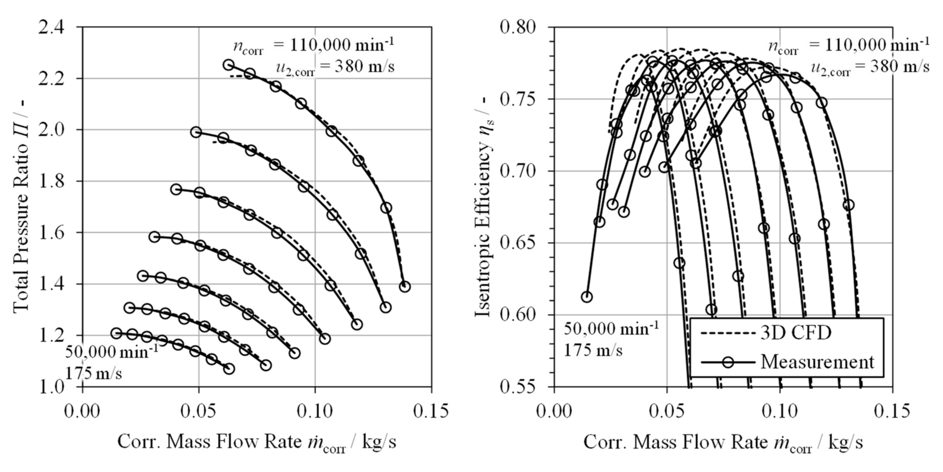
6.2. Experimental Results

Figure 19 compares the performance map measurements to the 3D CFDs simulation results determined for a model of the detailed compressor stage geometry (including test bench interfaces, measurement pipes and the as-machined impeller and housing geometry).

Very good agreement between simulation and measurement is achieved over the entire operating range:

$${\displaystyle \frac{\left|{\Pi }_{\mathrm{C}\mathrm{F}\mathrm{D}}-{\Pi }_{\mathrm{m}\mathrm{e}\mathrm{a}\mathrm{s}}\right|}{{\Pi }_{\mathrm{m}\mathrm{e}\mathrm{a}\mathrm{s}}}}\le 1.2\%\hspace{1em},\hspace{1em}\left|{\eta }_{\mathrm{s},\mathrm{C}\mathrm{F}\mathrm{D}}-{\eta }_{\mathrm{s},\mathrm{m}\mathrm{e}\mathrm{a}\mathrm{s}}\right|\le 2.5\%$$

(63)

The experimental results confirm the validity of the presented compressor design process. The optimization results can be assessed based on the measurement or simulation data. Figure 20 shows a comparison between the reference compressor used for the operating strategy optimization in Section 3 (base design) and the optimized compressor prototype.

Compared to the base design, the maximum isentropic compressor efficiency is increased by Δη_s,max = 7%. In the design point, Δη_s,des = 9.4% is achieved. The impeller diameter is reduced from d_2,base = 73 mm to d_2,prototype = 64 mm. Due to the lower impeller thrust load and higher design speed, the axial bearing diameter and associated friction losses can be reduced. This yields an effective compressor efficiency increase of Δη_eff,des = 12% in the design point.

On the PEM FC system level, this results in an efficiency increase of Δη_sys = 1.4% compared to the optimized operating strategy derived in Figure 6. Compared to the base system without operating strategy optimization, Δη_sys = 2.7% is achieved.

7. Summary and Conclusions

Based on the current state of research, this article provides a guideline for the design of cathode air compressors for PEM FC systems in mobile applications.

The efficiency optimal operating strategy of the PEM FC system and the resulting optimum operating line of the cathode air compressor ṁ_corr, Π = f (P_stack) are determined by means of a PEM FC system simulation. For this purpose, physically based models for the PEM FC stack and the membrane humidifier are introduced. These models accurately predict the operating behavior for varying operating boundary conditions (cathode stoichiometry, pressure, relative humidity). Based on the simulation results, the following qualitative statements can be made:

The influence of cathode stoichiometry and operating pressure on PEM FC efficiency increases with the current density. PEM FC systems operated at a high specific power have a correspondingly high boost pressure requirement. The boost pressure requirement and associated compressor power can be significantly reduced by increasing the number of cells in the PEM FC stack.

Proper PEM and GDL water balance is a prerequisite for good cell efficiency. By increasing the operating pressure, the relative humidity of the cathode air can be increased to ensure sufficient PEM conductivity and to offset the inadequate humidification performance of small membrane humidifiers.

To compensate for cell aging effects, the cathode air mass flow rate and stack operating pressure must be increased. For this purpose, the cathode air compressor must provide a sufficient map and power reserve.

Based on the design point determined in the system simulation, a preliminary design process for the cathode air compressor is developed, integrating the constraints of the electric machine and air bearing system (the power-to-speed trade-off and thrust load limit).

Starting from the preliminary design, a meanline performance model is used for automated compressor geometry optimization. The low computing time of the meanline performance model allows for an exploration of large design spaces. Flow phenomena that are only empirically approximated by the meanline performance model are resolved by 3D CFDs simulations during the detailed design phase.

To verify the operating behavior predicted by simulation, the optimized compressor geometry is implemented as a prototype and tested on a centrifugal compressor test stand. A sensor telemetry system is developed to measure the torque on the compressor drive shaft. This way, the isentropic compressor efficiency can be determined independent of the heat transfer between the working fluid and compressor housing. Compressor performance and efficiency predicted by the 3D CFDs simulations are subsequently confirmed with a high degree of accuracy (|η_s,CFD − η_s,meas ≤ 2.5%|).

To prove its validity, the proposed design process is carried out for an exemplary passenger car application. By means of operating strategy optimization alone, PEM FC system efficiency can be increased by Δη_sys = 1.3% without the need for hardware changes. The effective compressor efficiency of the optimized cathode air compressor is Δη_eff = 12% higher compared to the baseline compressor, yielding an overall PEM FC system efficiency gain of Δη_sys = 2.7%.

The requirements specified in Section 1 are fulfilled:

The detailed system simulation and the physically based component models foster a comprehensive understanding for the interaction of the individual components in the PEM FC system. Cathode air compressor design targets can be substantiated based on the system efficiency optimal operating strategy.

The preliminary design process provides a compressor geometry with close-to-optimum efficiency for a given PEM FC system while taking the design constraints of the electric compressor drive and air bearing system into account.

The high degree of integration and automation throughout the design process supports a rapid response to changing design requirements. The time and resources required for iteration loops are significantly reduced.

References

1. Thomas, C.E. Fuel cell and battery electric vehicles compared. Int. J. Hydrog. Energy 2009, 34, 6005–6020. [Google Scholar] [CrossRef]
2. Dicks, L.; Rand, D.A.J. Fuel Cell Systems Explained, 3rd ed.; Wiley: Hoboken, NJ, USA, 2018. [Google Scholar]
3. Dixon, S.L.; Hall, C.A. Fluid Mechanics and Thermodynamics of Turbomachinery; Elsevier: Amsterdam, The Netherlands, 2010. [Google Scholar]
4. Schloßhauer. Erweiterung der Kennfeldbasierten Verdichtermodellierung für Sequentielle Aufladesysteme. Ph.D. Dissertation, RWTH Aachen University, Aachen, Germany, 2021. [Google Scholar]
5. Luczynski, P.; Hohenberg, K.; Freytag, C.; Martinez-Botas, R. Integrated Design Optimisation and Engine Matching of a Turbocharger Radial Turbine. In Proceedings of the 14th International Conference on Turbochargers and Turbocharging; CRC Press: London, UK, 2021. [Google Scholar]
6. Uhlmann, T. Vermessung und Modellierung von Abgasturboladern für Die Motorprozessrechnung. Ph.D. Thesis, RWTH Aachen University, Aachen, Germany, 2013. [Google Scholar]
7. Lückmann, D. Interaktion Zweiflutiger Turbinen Mit Dem Verbrennungsmotor. Ph.D. Thesis, RWTH Aachen University, Aachen, Germany, 2016. [Google Scholar]
8. Pfleiderer. Die Kreiselpumpen für Flüssigkeiten und Gase—Wasserpumpen, Ventilatoren, Turbogebläse—5. Neubearbeitete Auflage; Springer: Berlin/Göttingen/Heidelberg, Germany, 1961. [Google Scholar]
9. Allard. Turbocharging & Supercharging; Cornell University: Ithaca, NY, USA, 1986. [Google Scholar]
10. Giakoumis, E.G. Turbochargers and Turbocharging—Advancements, Applications and Research; Nova Science Publishers: Hauppauge, NY, USA, 2017. [Google Scholar]
11. Klütsch, J.; Pischinger, S.; Lückmann, D.; Schloßhauer, A. Simulation-Driven Fuel Cell Compressor Design. MTZ Mot. Z. 2021, 82, 28–37. [Google Scholar] [CrossRef]
12. Gerada, D.; Mebarki, A.; Brown, N.L.; Gerada, C.; Cavagnino, A.; Boglietti, A. High-Speed Electrical Machines: Technologies, Trends, and Developments. IEEE Trans. Ind. Electron. 2014, 61, 2946–2959. [Google Scholar] [CrossRef]
13. Dellacorte, C.; Valco, M.J. Load Capacity Estimation of Foil Air Journal Bearings for Oil-Free Turbomachinery Applications. Tribol. Trans. 2000, 43, 795–801. [Google Scholar] [CrossRef]
14. Klütsch, J.; Stadermann, M.; Lückmann, D.; Schloßhauer, A.; Walters, M. Fuel Cell Air Compressor Design for Mobile Applications. In Proceedings of the 26th Supercharging Conference, Dresden, Germany, 20–21 September 2022. [Google Scholar]
15. Kim, J.; Lee, S.-M.; Srinivasan, S.; Chamberlin, C.E. Modeling of Proton Exchange Membrane Fuel Cell Performance with an Empirical Equation. J. Electrochem. Soc. 1995, 142, 2670. [Google Scholar] [CrossRef]
16. Haslinger, M.; Lauer, T. Unsteady 3D-CFD Simulation of a Large Active Area PEM Fuel Cell under Automotive Operation Conditions—Efficient Parameterization and Simulation Using Numerically Reduced Models. Processes 2022, 10, 1605. [Google Scholar] [CrossRef]
17. Houreh, N.B.; Afshari, E. Three-dimensional CFD modeling of a planar membrane humidifier for PEM fuel cell systems. Int. J. Hydrog. Energy 2014, 39, 14969–14979. [Google Scholar] [CrossRef]
18. Oertel, H. Prandtl’s Essentials of Fluid Mechanics, 2nd ed.; Springer: New York, NY, USA; Berlin/Heidelberg, Germany, 2004. [Google Scholar]
19. Moody, L.F. Friction Factors for Pipe Flow. Trans. ASME 1944, 66, 671–684. [Google Scholar] [CrossRef]
20. Fick. Über Diffusion. Poggendorff’s Ann. Der Phys. 1855, 94, 59–86. [Google Scholar]
21. Kulikovsky, A. Analytical Modelling of Fuel Cells; Elsevier: Amsterdam, The Netherlands, 2010. [Google Scholar]
22. Jamekhorshid, A.; Karimi, G.; Noshadi, I. Current Distribution and Cathode Flooding Prediction in a PEM Fuel Cell. Int. J. Chem. Mol. Energy 2010, 4, 157–165. [Google Scholar] [CrossRef]
23. Liu, Z.; Mao, Z.; Wang, C. A two dimensional partial flooding model for PEMFC. J. Power Sources 2006, 158, 1229–1239. [Google Scholar] [CrossRef]
24. Bakhtiar, A.; Kim, Y.-B.; You, J.-K.; Yoon, J.-I.; Choi, K.-H. A model and simulation of cathode flooding and drying on unsteady proton exchange membrane fuel cell. J. Cent. South Univ. 2012, 19, 2572–2577. [Google Scholar] [CrossRef]
25. Springer, T.E.; Zawodzinski, T.A.; Gottesfeld, S. Polymer Electrolyte Fuel Cell Model. J. Electrochem. Soc. 1991, 138, 2334–2342. [Google Scholar] [CrossRef]
26. Lee, J.S.; Quan, N.D.; Hwang, J.M.; Lee, S.D.; Kim, H.; Lee, H.; Kim, H.S. Polymer Electrolyte Membranes for Fuel Cells. J. Ind. Eng. Chem. 2006, 12, 175–183. [Google Scholar] [CrossRef]
27. Zook, L.A.; Leddy, J. Density and Solubility of Nafion: Recast, Annealed, and Commercial Films. Anal. Chem. 1996, 68, 3793–3796. [Google Scholar] [CrossRef] [PubMed]
28. Kulikovsky, A. Quasi-3D Modeling of Water Transport in Polymer Electrolyte Fuel Cells. J. Electrochem. Soc. 2003, 150, A1432–A1439. [Google Scholar] [CrossRef]
29. Van Bussel, H.P.; Koene, F.G.; Mallant, R.K. Dynamic model of solid polymer fuel cell water management. J. Power Sources 1998, 71, 218–222. [Google Scholar] [CrossRef]
30. FEV Europe GmbH. Vehicle Benchmark Hyundai Nexo, Final Report; FEV Europe GmbH: Aachen, Germany, 2020. [Google Scholar]
31. FEV Europe GmbH. Vehicle Benchmark Toyota Mirai 2, Final Report; FEV Europe GmbH: Aachen, Germany, 2021. [Google Scholar]
32. Tinz, S.N. Befeuchtungskonzepte für Brennstoffzellensysteme in Mobilen Anwendungen. Ph.D. Thesis, RWTH Aachen University, Aachen, Germany, 2022. [Google Scholar]
33. Bird, R.B.; Steward, W.E.; Lightfoot, E.N. Transport Phenomena, 2nd ed.; Wiley: Hoboken, NJ, USA, 2007. [Google Scholar]
34. Colburn, P. A Method of Correlating Forced Convection Heat Transfer Data and A Comparison with Fluid Friction. Int. J. Heat Mass Transf. 1933, 6, 1359–1384. [Google Scholar] [CrossRef]
35. White, M. Viscous Fluid Flow, 2nd ed.; McGraw-Hill, Inc.: New York, NY, USA, 1991. [Google Scholar]
36. Buhmann, M.D. Radial Basis Functions—Theory and Implementations; Cambridge University Press: Cambridge, UK, 2003. [Google Scholar]
37. Wick, M.; Klütsch, J.; Walters, M.; Zubel, M.; Jesser, M.; Ogrzewalla, J.; Schloßhauer, A.; Lückmann, D.; Uhlmann, T.; van der Put, D.; et al. 300+ kW Brennstoffzellensysteme für den Fernverkehr—Welche Verbesserungen sind mit dieser nächsten Generation von Brennstoffzellensystemen zu erwarten? In 44. Internationales Wiener Motorensymposium; Foreign Trade Center Budapest: Wien, NY, USA, 2023. [Google Scholar]
38. Mayur, M.; Gerard, M.; Schott, P.; Bessler, W.G. Lifetime Prediction of a Polymer Electrolyte Membrane Fuel Cell under Automotive Load Cycling Using a Physically-Based Catalyst Degradation Model. Energies 2018, 11, 2054. [Google Scholar] [CrossRef]
39. Wu, J.; Yuan, X.Z.; Martin, J.J.; Wang, H.; Zhang, J. A review of PEM fuel cell durability: Degradation mechanisms and mitigation strategies. J. Power Sources 2008, 184, 104–119. [Google Scholar] [CrossRef]
40. Yousfi-Steiner, N.; Mocotéguy, P.; Candusso, D.; Hissel, D. A review on polymer electrolyte membrane fuel cell catalyst degradation and starvation issues: Causes, consequences and diagnostic for mitigation. J. Power Sources 2009, 194, 130–145. [Google Scholar] [CrossRef]
41. US Department of Energy—Hydrogen and Fuel Cell Technologies Office. DOE Technical Targets for Polymer Electrolyte Membrane Fuel Cell Components. Available online: https://www.energy.gov/eere/fuelcells/doe-technical-targets-polymer-electrolyte-membrane-fuel-cell-components (accessed on 22 August 2022).
42. Aungier, R.H. Centrifugal Compressors—A Strategy for Aerodynamic Design and Analysis; The American Society of Mechanical Engineers: New York, NY, USA, 2000. [Google Scholar]
43. Rusch, D.; Casey, M. The Design Space Boundaries for High Flow Capacity Centrifugal Compressors. J. Turbomach. 2013, 135, 031035. [Google Scholar] [CrossRef]
44. Casey, M.V.; Schlegel, M. Estimation of the performance of turbocharger compressors at extremely low pressure ratios. Proc. Inst. Mech. Eng. Part A J. Power Energy 2010, 224, 239–250. [Google Scholar] [CrossRef]
45. Wiesner, J. A Review of Slip Factors for Centrifugal Impellers. J. Eng. Power 1967, 89, 558–566. [Google Scholar] [CrossRef]
46. Stodola, A. Steam and Gas Turbines; McGraw-Hill: New York, NY, USA, 1927. [Google Scholar]
47. Senoo, Y.; Kinoshita, Y. Limits of Rotating Stall and Stall in Vaneless Diffuser of Centrifugal Compressors. In ASME 1978 International Gas Turbine Conference and Products Show; American Society of Mechanical Engineers: London, UK, 1978. [Google Scholar]
48. Wu, C.-H. A General Theory of Two- and Three-Dimensional Rotational Flow in Subsonic and Transonic Turbomachines, NASA Contractor Report 4496. In Nasa Scientific and Technical Information Program; NTRS—NASA Technical Reports Server: Cleveland, OH, USA, 1993. [Google Scholar]
49. Japikse, D. Centrifugal Compressor Design and Performance, White River Junction; Concepts ETI: Wilder, TN, USA, 1996. [Google Scholar]
50. Klütsch, J.; Wick, M.; Schloßhauer, A.; Lückmann, D.; Walters, M. Simulation-Driven PEM Fuel Cell Compressor Design. In Proceedings of the 30th Aachen Colloquium Sustainable Mobility 2021, Aachen, Germany, 4–6 October 2021. [Google Scholar]
51. Müller, K.V.; Ponick, B. Berechnung Elektrischer Maschinen, 6. Auflage; Wiley-VCH: Berlin, Germany, 2007. [Google Scholar]
52. Pyrhönen, J.; Jokinen, T.; Hrabovcova, V. Design of Rotating Electrical Machines, 2nd ed.; John Wiley & Sons, Inc.: Hoboken, NJ, USA, 2013. [Google Scholar]
53. Binder, A. Motor Development for Electrical Drive Systems—High Speed PM Machines; Institut für Elektrische Energiewandlung: Darmstadt, Germany, 2017. [Google Scholar]
54. Dykas, B.; Bruckner, R.; DellaCorte, C.; Edmonds, B.; Prahl, J. Design, Fabrication, and Performance of Foil Gas Thrust Bearings for Microturbomachinery Applications; Nasa Technical Memo: Cleveland, OH, USA, 2008. [Google Scholar]
55. DellaCorte, C.; Radil, K.C.; Bruckner, R.J.; Howard, S.A. Design, Fabrication, and Performance of Open Source Generation I and II Compliant Hydrodynamic Gas Foil Bearings. Tribol. Trans. 2008, 51, 254–264. [Google Scholar] [CrossRef]
56. Kim, T.H.; Park, M.; Lee, T.W. Design Optimization of Gas Foil Thrust Bearings for Maximum Load Capacity. J. Tribol. 2017, 139, 031705. [Google Scholar] [CrossRef]
57. Zhang, J.; Sun, H.; Hu, L.; He, H. Fault Diagnosis and Failure Prediction by Thrust Load Analysis for a Turbocharger Thrust Bearing. In ASME Turbo Expo 2010: Power for Land, Sea and Air; ASME: Glasgow, UK, 2010. [Google Scholar]
58. Bahm, F.U. Das Axialschubverhalten von Einstufigen Kreiselpumpen mit Spiralgehäuse. Ph.D. Thesis, Universität Hannover, Hannover, Germany, 2000. [Google Scholar]
59. Honda, H.; Kanzaka, T.; Oka, N.; Verstraete, T.; Châtel, A.; Müller, L. Performance improvement of centrifugal compressors for automotive turbochargers using adjoint method. In 16th Asian International Conference on Fluid Machinery; IOP Publishing: Bristol, UK, 2021. [Google Scholar]
60. Wang, X.-F.; Wang, G.; Wang, Z.H. Aerodynamic optimization design of centrifugal compressor’s impeller with Kriging model. Proc. Inst. Mech. Eng. Part A J. Power Energy 2006, 220, 589–597. [Google Scholar] [CrossRef]
61. Siemens Digital Industries Software. Simcenter STAR-CCM+ Software. Available online: https://plm.sw.siemens.com/de-DE/simcenter/fluids-thermal-simulation/star-ccm/ (accessed on 29 June 2024).
62. Rotrex A/S. C30 Technical Data Sheet, Rev. 6.0. 01 2022. Available online: https://www.rotrex.com/wp-content/uploads/2022/01/Rotrex-Technical-Datasheet-C30-Rev6.0.pdf (accessed on 8 May 2023).
63. SAE Engine Power Test Code Committee, J1826-202204—Turbocharger Gas Stand Test Code; SAE International: Warrendale PA, USA, 2022.
64. Björn, H. Analyse und Modellierung des thermischen Verhaltens von Pkw-Abgasturboladern. Ph.D. Thesis, RWTH Aachen University, Aachen, Germany, 2017. [Google Scholar]
65. Klütsch, J.P.; Brodbeck, P.; Winkler, H. Bedatung von Modellen zur Beschreibung des Betriebsverhaltens von Abgasturboladern; FVV1314, Final Report; Forschungsvereinigung Verbrennungskraftmaschinen e. V.: Frankfurt am Main, Germany, 2020. [Google Scholar]
66. Kistler Instrumente, A.G. Torque Sensor with Dual-Range-Option Type 4503B. Available online: https://kistler.cdn.celum.cloud/SAPCommerce_Download_original/000-767e.pdf (accessed on 3 May 2023).
67. Manner Sensortelemetrie GmbH. Sensor Signal Amplifier Type RMC Samy-Flex—Technical Datasheet. Available online: https://www.sensortelemetrie.de/wp-content/uploads/technical_datasheet_signalverstrker_samy-flex.pdf (accessed on 3 May 2023).
Figure 1. PEM FC finite volume model with substance transport and discretization grid.
Energies 17 03534 g001
Figure 2. Stationary PEM FC model results for variations of operating boundary conditions.
Energies 17 03534 g002
Figure 3. Gas and water transport in the membrane humidifier.
Energies 17 03534 g003
Figure 4. Exemplary membrane humidifier model results (left) and comparison between measurement and model results for mass flow rate and pressure variation (right). All results are for cross-flow arrangement.
Energies 17 03534 g004
Figure 5. PEM FC system model schematic.
Energies 17 03534 g005
Figure 6. PEM FC system efficiency optimal cathode air compressor operating points for varying stack power levels (optimum operating line) determined with the stationary PEM FC system model.
Energies 17 03534 g006
Figure 7. PEM FC stack size variation study results.
Energies 17 03534 g007
Figure 8. Membrane humidifier size variation study results.
Energies 17 03534 g008
Figure 9. US DoE aging criteria in dependence of active cell area (left) and feasible compressor map range for aged PEM FC system (right).
Energies 17 03534 g009
Figure 10. Polytropic compressor efficiency estimate according to Equation (30) for varying design flow parameters and impeller tip diameters.
Energies 17 03534 g010
Figure 11. Absolute and relative flow velocity components in meridional coordinate system at impeller inlet and impeller tip.
Energies 17 03534 g011
Figure 12. Relative Mach number and blade angle at impeller inlet for incidence-free flow at varying inlet eye diameters and design speeds.
Energies 17 03534 g012
Figure 13. Design speed lines for varying impeller tip blade angles and blade heights (β2, b2 = f(α2), cu2 = const.).
Energies 17 03534 g013
Figure 14. Preliminary compressor design results: required and achievable electric machine power (left) and estimates for compressor efficiency and impeller tip diameter (right).
Energies 17 03534 g014
Figure 15. Selection chart for electrically driven PEM FC cathode air compressors.
Energies 17 03534 g015
Figure 16. Meanline performance model results for selected design candidates with highlighted optimum design candidate compared to base reference design and preliminary design candidate.
Energies 17 03534 g016
Figure 17. Compressor performance map comparison between the optimum design candidate found by the initial meanline performance model optimization and the result of 3D CFDs optimization.
Energies 17 03534 g017
Figure 18. Electrically driven centrifugal compressor test stand.
Energies 17 03534 g018
Figure 19. Comparison of performance map measurement (centrifugal compressor test stand with torque sensor) to 3D CFDs simulation results (full-stage model including test bench interfaces).
Energies 17 03534 g019
Figure 20. Base design and optimized compressor prototype: performance map comparison (left) and PEM FC system level performance for operating strategy and compressor geometry optimization (right).
Energies 17 03534 g020
Disclaimer/Publisher’s Note: The statements, opinions and data contained in all publications are solely those of the individual author(s) and contributor(s) and not of MDPI and/or the editor(s). MDPI and/or the editor(s) disclaim responsibility for any injury to people or property resulting from any ideas, methods, instructions or products referred to in the content.