
Analysis of Wind Resource Characteristics in the Ulanqab Wind Power Base (Wind Farm): Mesoscale Modeling Approach

Abstract
:1. Introduction
2. Overview of the Ulanqab Wind Power Base and Experimental Design
2.1. Basic Information about the Wind Power Base
2.2. Selection of Parameterization Schemes
2.3. Experimental Design
3. Grid Horizontal Resolution Selection
4. Results and Discussion
5. Conclusions
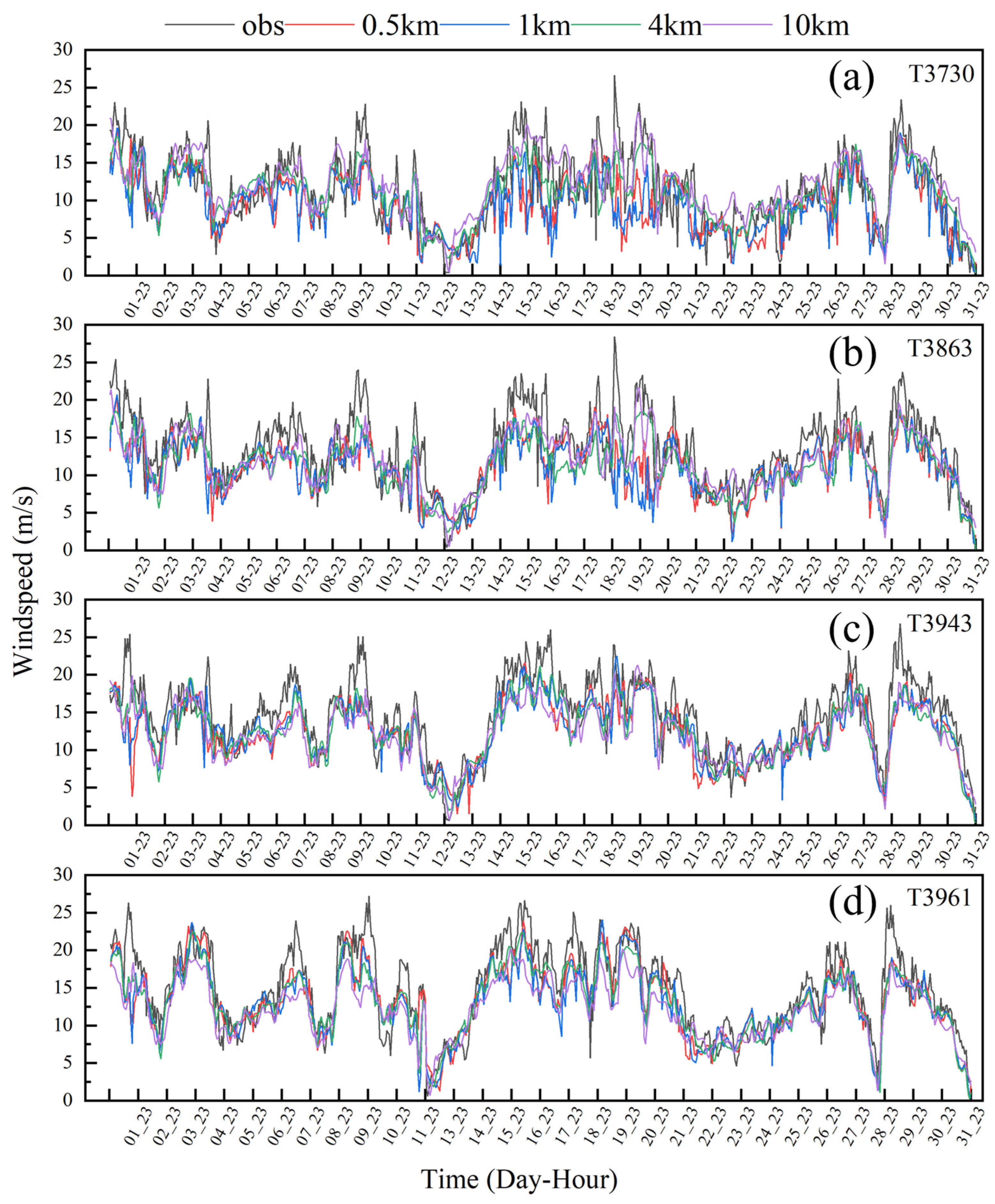
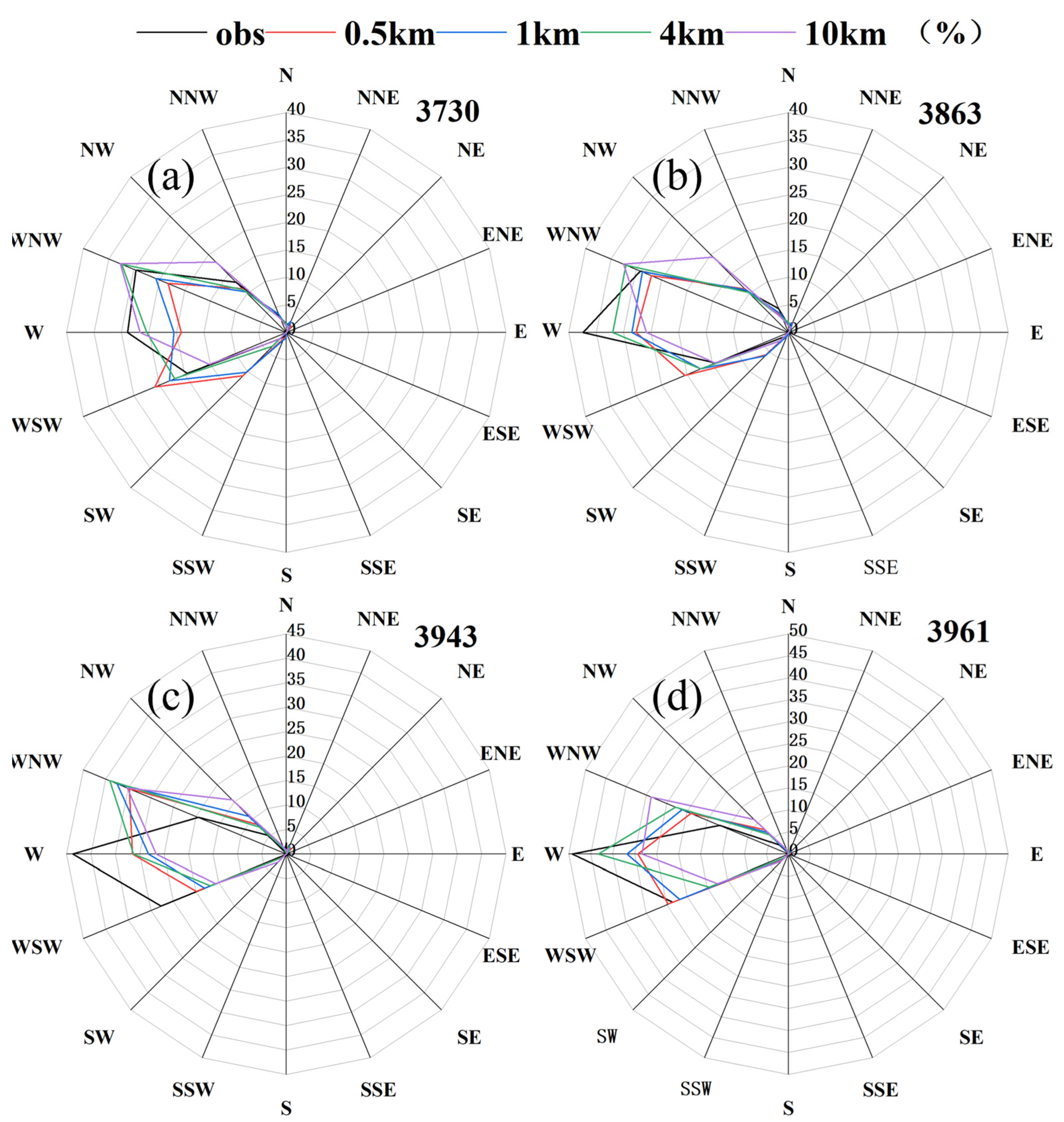
- Overly fine horizontal resolution can lead to underestimations of wind speed. Conducting mesoscale simulations of large wind power bases at a 4 km horizontal resolution can adequately balance the calculation accuracy of both wind speed and direction while requiring fewer computational resources, making it more suitable for practical engineering applications.
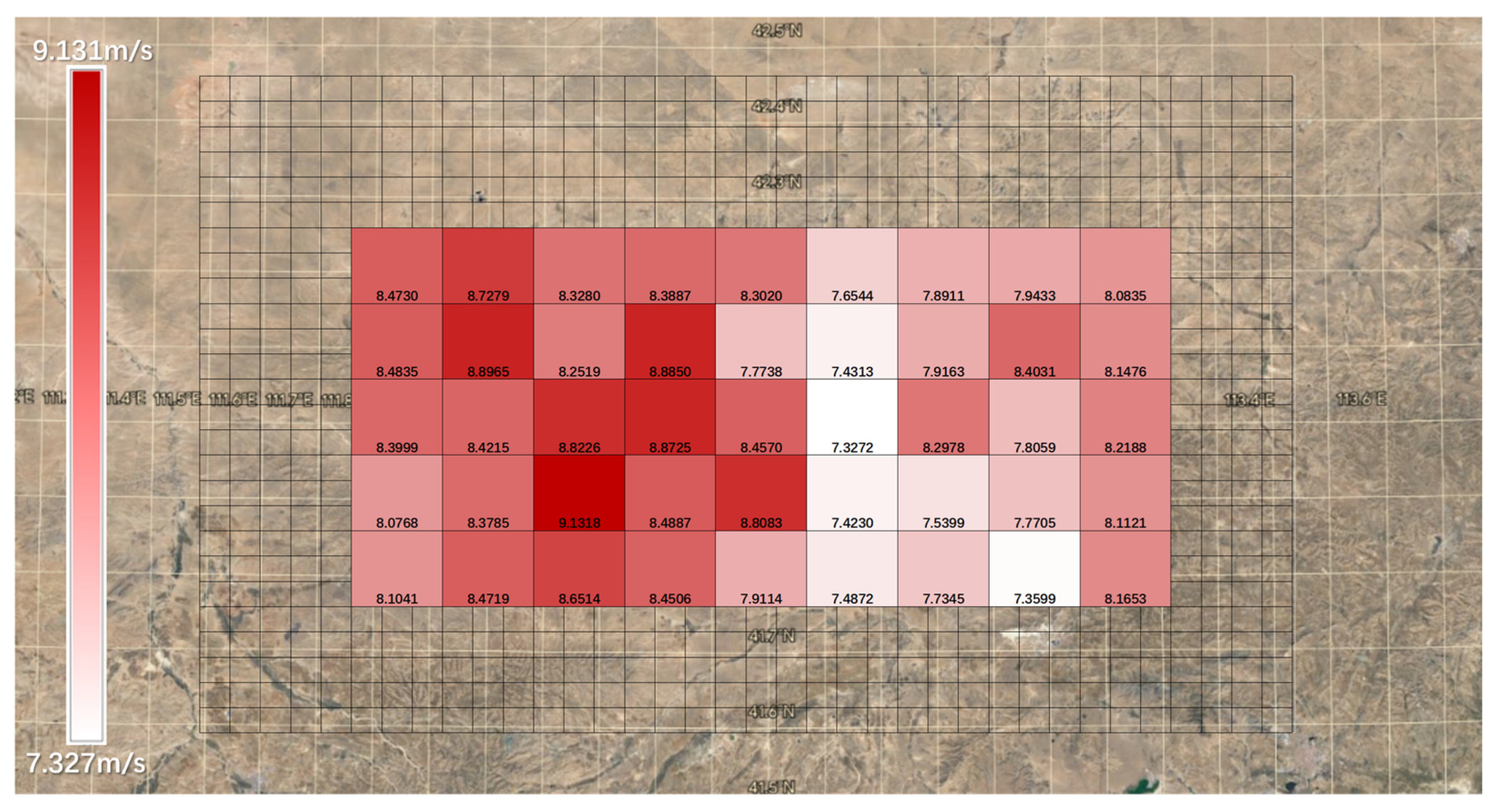
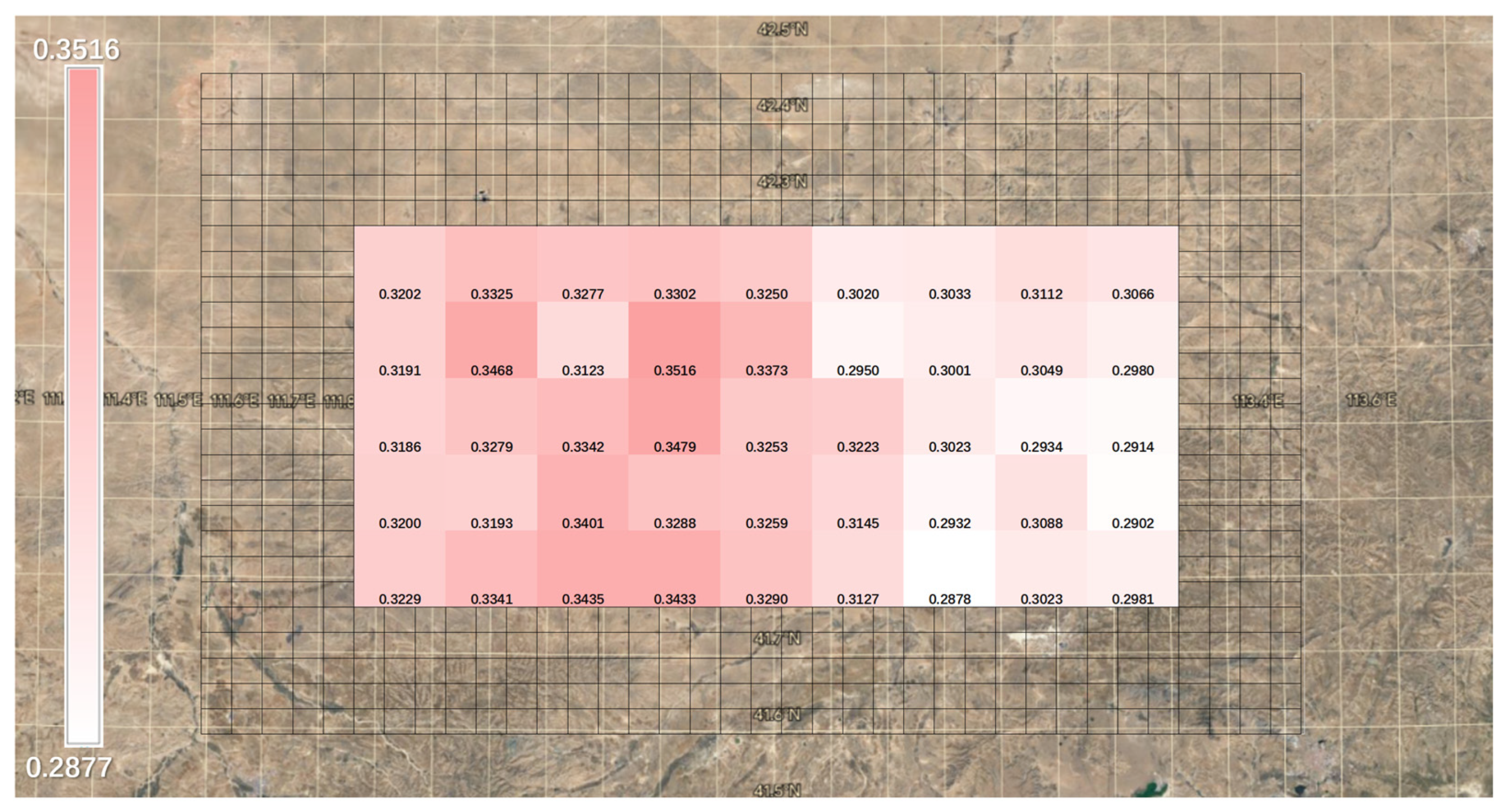
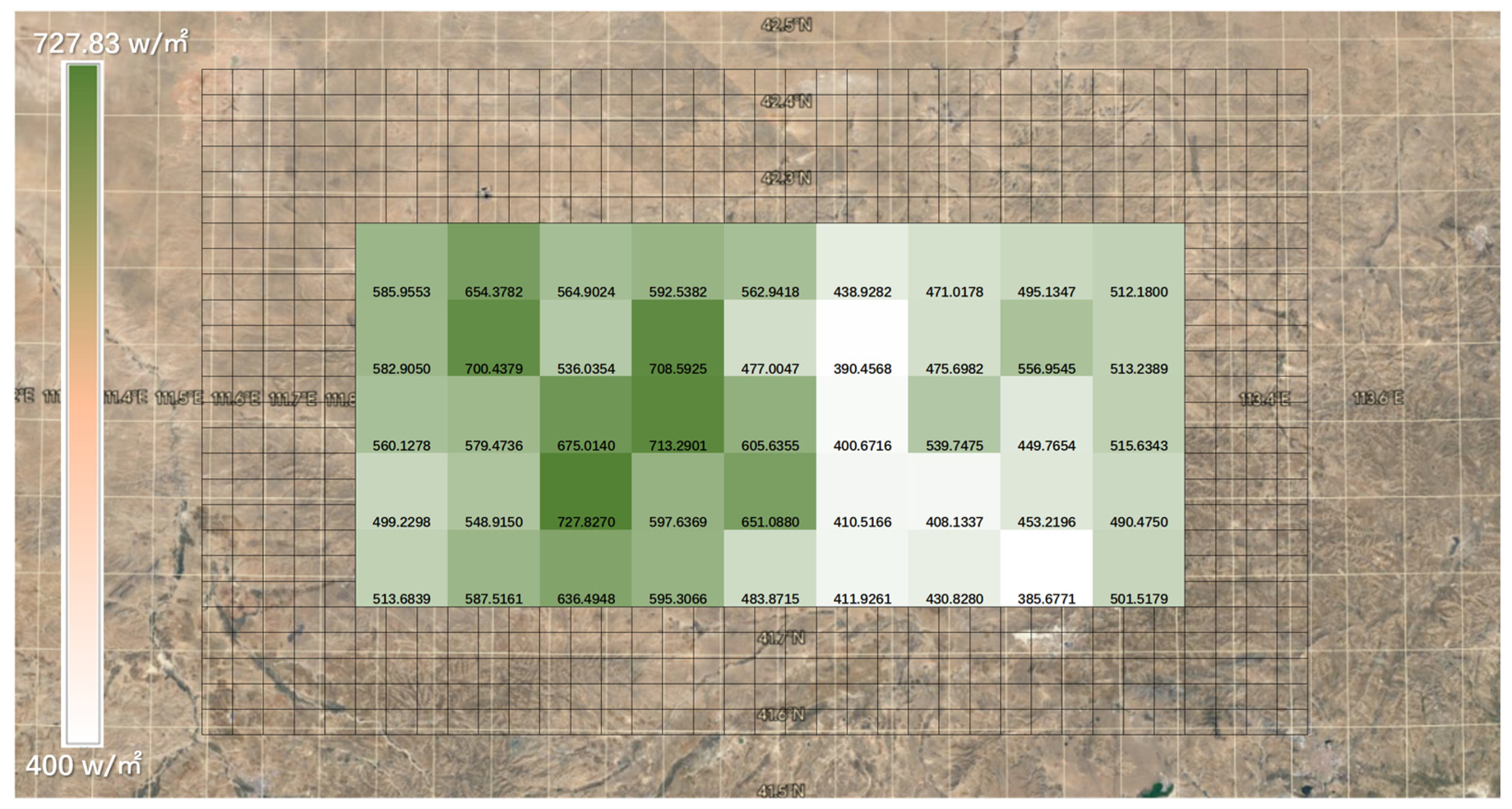
- In the Ulanqab wind power base area, the annual average wind speed ranges from 7.327 to 9.131 m/s; turbulence intensity ranges from 0.2877 to 0.3516; the measured values for annual average wind power density range from 400 to 727.83 W/m2; and the wind power density level is between 5 and 6. The wind speed is at a high level with minimal fluctuation, showing great potential for wind energy development and suitability for the operation of wind energy equipment.
- In the Ulanqab wind power base, an equidistant layout is recommended for flat terrains to maximize the wind farm’s coverage area. In complex terrains, adjusting the height of wind turbines is more crucial. Increasing the height appropriately can avoid significant impacts of terrain obstacles on wind speed, reduce blocking effects between turbines, and ensure that turbines fully capture wind resources.
Author Contributions
Funding
Data Availability Statement
Conflicts of Interest
Appendix A

| (a) | |||
| Month | MAE/m·s−1 | RMSE/m·s−1 | Relative Error |
| 2010-6 | 0.972069 | 1.369005 | 12.2970% |
| 2010-7 | 1.495390 | 1.746474 | 18.6485% |
| 2010-8 | 1.308750 | 1.649963 | 14.7526% |
| 2010-9 | 1.647514 | 2.064556 | 23.2959% |
| 2010-10 | 1.562406 | 1.998417 | 18.8081% |
| 2010-11 | 4.313819 | 4.895117 | 35.9706% |
| 2010-12 | 4.551573 | 5.134456 | 32.9202% |
| 2011-1 | 2.889409 | 3.516756 | 24.5647% |
| 2011-2 | 2.308289 | 2.797178 | 28.2564% |
| 2011-3 | 2.670712 | 3.471115 | 25.6852% |
| 2011-4 | 2.007764 | 2.466143 | 20.1443% |
| (b) | |||
| Month | MAE/m·s−1 | RMSE/m·s−1 | Relative Error |
| 2010-6 | 0.975875 | 1.138758 | 3.1128% |
| 2010-7 | 1.103737 | 1.363543 | 8.1692% |
| 2010-8 | 1.273253 | 1.568894 | 12.5209% |
| 2010-10 | 1.306962 | 1.686762 | 8.1646% |
| 2010-11 | 3.432262 | 3.976806 | 26.3689% |
| 2010-12 | 4.380236 | 5.211806 | 30.7107% |
| 2011-1 | 2.423528 | 3.139413 | 23.3169% |
| 2011-2 | 1.929970 | 2.721654 | 18.9256% |
| 2011-3 | 1.544019 | 2.098699 | 9.5772% |
| 2011-4 | 1.554972 | 2.036902 | 8.4051% |
| 2011-5 | 1.758212 | 2.374027 | 11.8054% |
| (c) | |||
| Month | MAE/m·s−1 | RMSE/m·s−1 | Relative Error |
| 2010-6 | 1.149926 | 1.440707 | 13.7023% |
| 2010-7 | 0.896465 | 1.085559 | 7.8385% |
| 2010-8 | 0.811815 | 1.018458 | 8.4693% |
| 2010-9 | 0.901653 | 1.171947 | 6.5620% |
| 2010-10 | 0.736868 | 0.847517 | 6.9692% |
| 2010-11 | 0.859207 | 1.119949 | 5.2778% |
| 2010-12 | 1.414489 | 1.969661 | 7.1658% |
| 2011-1 | 1.055269 | 1.244386 | 3.6111% |
| 2011-2 | 0.867202 | 1.017738 | 6.5577% |
| 2011-3 | 0.865430 | 1.099365 | 2.5069% |
| 2011-4 | 0.739083 | 0.964227 | 0.0835% |
| 2011-5 | 1.005188 | 1.307421 | 1.3272% |
| (d) | |||
| Month | MAE/m·s−1 | RMSE/m·s−1 | Relative Error |
| 2010-6 | 0.828918 | 1.040576 | 0.2558% |
| 2010-7 | 0.96957 | 1.225748 | 4.5730% |
| 2010-8 | 0.830148 | 1.088485 | 6.4043% |
| 2010-9 | 1.047621 | 1.315122 | 6.4676% |
| 2010-10 | 0.996989 | 1.225163 | 8.4948% |
| 2010-11 | 2.320954 | 2.621755 | 20.9120% |
| 2010-12 | 3.075726 | 3.441829 | 23.6107% |
| 2011-1 | 2.244288 | 2.678956 | 19.2064% |
| 2011-2 | 1.355417 | 1.665421 | 12.9593% |
| 2011-3 | 1.850645 | 2.187967 | 17.2335% |
| 2011-4 | 1.17828 | 1.455611 | 11.1761% |
| 2011-5 | 1.463266 | 1.916806 | 12.0390% |
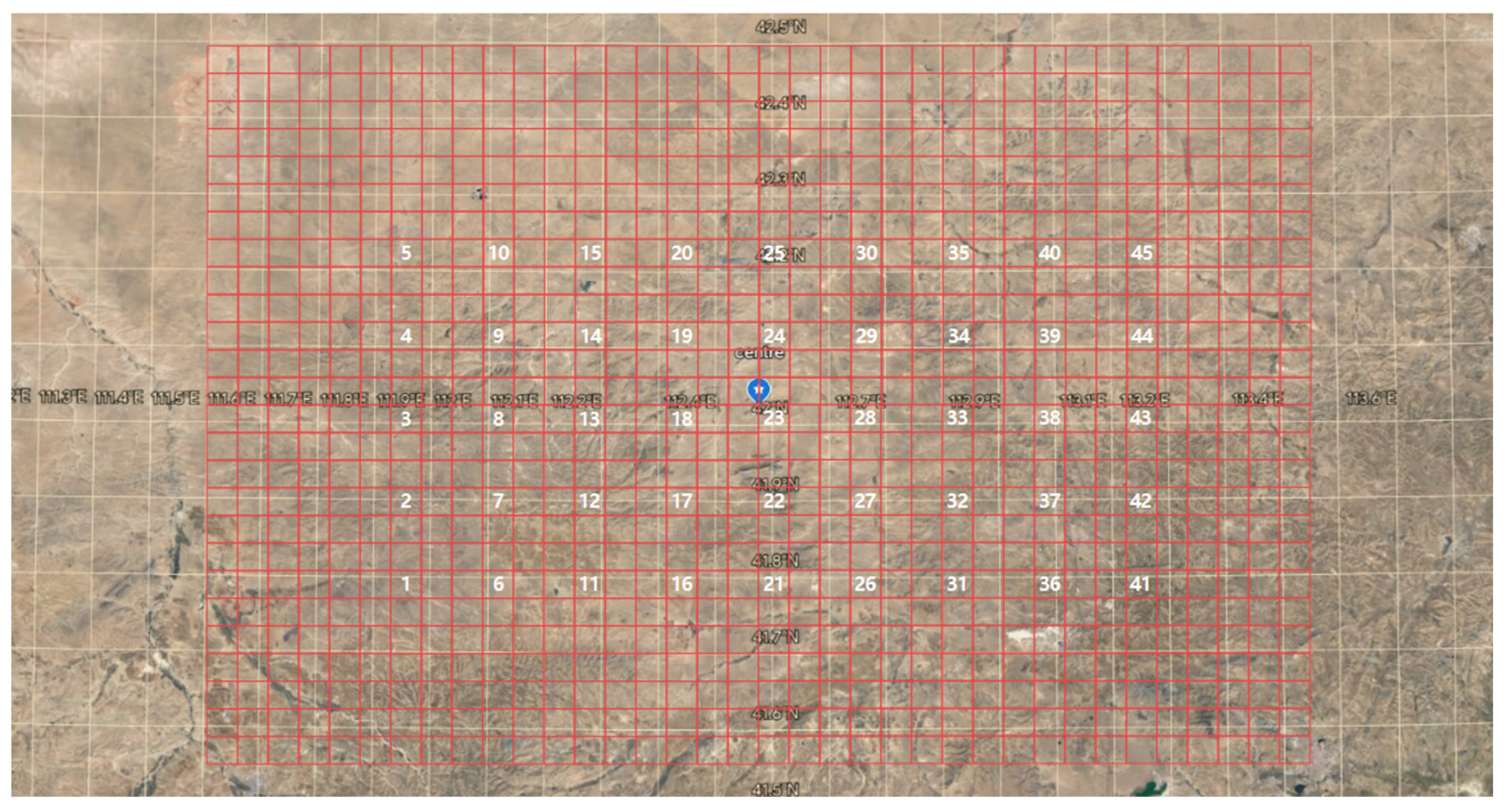
| Point Number | Longitude/° | Latitude/° |
|---|---|---|
| 1 | 112.0026 | 41.77696 |
| 2 | 112.0015 | 41.88849 |
| 3 | 112.0004 | 42.00002 |
| 4 | 112.0009 | 42.11265 |
| 5 | 111.9982 | 42.22314 |
| 6 | 111.9982 | 42.22314 |
| 7 | 111.9982 | 42.22314 |
| 8 | 111.9982 | 42.22314 |
| 9 | 112.1498 | 42.11224 |
| 10 | 112.149 | 42.22381 |
| 11 | 112.3017 | 41.77807 |
| 12 | 112.3012 | 41.88959 |
| 13 | 112.3007 | 42.00114 |
| 14 | 112.3002 | 42.11269 |
| 15 | 112.2997 | 42.22426 |
| 16 | 112.4513 | 41.77831 |
| 17 | 112.4511 | 41.88984 |
| 18 | 112.4509 | 42.00139 |
| 19 | 112.4506 | 42.11293 |
| 20 | 112.4504 | 42.22451 |
| 21 | 112.6009 | 41.77834 |
| 22 | 112.601 | 41.88987 |
| 23 | 112.601 | 42.00143 |
| 24 | 112.6011 | 42.11298 |
| 25 | 112.6011 | 42.22455 |
| 26 | 112.7505 | 41.77818 |
| 27 | 112.7509 | 41.88971 |
| 28 | 112.7512 | 42.00124 |
| 29 | 112.7515 | 42.1128 |
| 30 | 112.7518 | 42.22437 |
| 31 | 112.9001 | 41.77779 |
| 32 | 112.9007 | 41.88932 |
| 33 | 112.9013 | 42.00087 |
| 34 | 112.9019 | 42.11242 |
| 35 | 112.9025 | 42.22397 |
| 36 | 113.0497 | 41.77721 |
| 37 | 113.0506 | 41.88873 |
| 38 | 113.0515 | 42.00027 |
| 39 | 113.0524 | 42.11182 |
| 40 | 113.0533 | 42.22339 |
| 41 | 113.1993 | 41.7764 |
| 42 | 113.2004 | 41.88792 |
| 43 | 113.2016 | 41.99947 |
| 44 | 113.2028 | 42.11102 |
| 45 | 113.204 | 42.22258 |
| Point Numbe | Annual Average Wind Speed/m·s−1 | Turbulence Intensity | Annual Average Wind Power Density/W·m−2 |
|---|---|---|---|
| 1 | 8.1041101 | 0.3229286 | 513.6839459 |
| 2 | 8.0767585 | 0.3199952 | 499.2297909 |
| 3 | 8.3998524 | 0.3186319 | 560.1277942 |
| 4 | 8.483543 | 0.319104 | 582.9049902 |
| 5 | 8.472975 | 0.320163 | 585.9553334 |
| 6 | 8.471918 | 0.334064 | 587.5160964 |
| 7 | 8.378492 | 0.319339 | 548.9150254 |
| 8 | 8.421547 | 0.327882 | 579.4736091 |
| 9 | 8.896453 | 0.346759 | 700.437858 |
| 10 | 8.727921 | 0.33253 | 654.3782222 |
| 11 | 8.651424 | 0.343526 | 636.4947688 |
| 12 | 9.131844 | 0.340107 | 727.8269875 |
| 13 | 8.822581 | 0.334211 | 675.0139863 |
| 14 | 8.251927 | 0.312326 | 536.0354253 |
| 15 | 8.327987 | 0.32769 | 564.9023567 |
| 16 | 8.450591 | 0.343339 | 595.3066167 |
| 17 | 8.488663 | 0.328766 | 597.6369231 |
| 18 | 8.872523 | 0.34792 | 713.2900586 |
| 19 | 8.88502 | 0.351634 | 708.592505 |
| 20 | 8.388699 | 0.330233 | 592.538197 |
| 21 | 7.911385 | 0.328983 | 483.8715135 |
| 22 | 8.80834 | 0.325949 | 651.0879919 |
| 23 | 8.457009 | 0.325289 | 605.6354951 |
| 24 | 7.773824 | 0.337327 | 477.0047165 |
| 25 | 8.302027 | 0.325018 | 562.9418033 |
| 26 | 7.487173 | 0.31269 | 411.9261171 |
| 27 | 7.422982 | 0.314516 | 410.5165645 |
| 28 | 7.327178 | 0.322299 | 400.671643 |
| 29 | 7.43128 | 0.295024 | 390.4567518 |
| 30 | 7.654353 | 0.301992 | 438.9282381 |
| 31 | 7.359871 | 0.302284 | 385.6770955 |
| 32 | 7.770468 | 0.308827 | 453.2196023 |
| 33 | 7.805937 | 0.293372 | 449.7654077 |
| 34 | 8.403074 | 0.304882 | 556.9544909 |
| 35 | 7.943344 | 0.31121 | 495.1347244 |
| 36 | 7.734493 | 0.28777 | 430.8280079 |
| 37 | 7.539879 | 0.293231 | 408.1337379 |
| 38 | 8.297772 | 0.302325 | 539.747534 |
| 39 | 7.916337 | 0.300147 | 475.6981808 |
| 40 | 7.891123 | 0.303338 | 471.0177723 |
| 41 | 8.165283 | 0.298124 | 501.5179189 |
| 42 | 8.112145 | 0.290225 | 490.4749924 |
| 43 | 8.218756 | 0.291404 | 515.6343216 |
| 44 | 8.147643 | 0.298013 | 513.238947 |
| 45 | 8.083455 | 0.306622 | 512.1800006 |
| Number | Azimuth Angle Frequency | N | NNE | NE | ENE |
|---|---|---|---|---|---|
| 1 | 0.14 | 0.179 | 0.098 | 0.047 | |
| 2 | 0.139 | 0.191 | 0.1 | 0.045 | |
| 3 | 0.165 | 0.188 | 0.089 | 0.042 | |
| 4 | 0.192 | 0.17 | 0.078 | 0.039 | |
| 5 | 0.209 | 0.148 | 0.072 | 0.042 | |
| 6 | 0.17 | 0.204 | 0.099 | 0.044 | |
| 7 | 0.158 | 0.198 | 0.103 | 0.048 | |
| 8 | 0.169 | 0.158 | 0.075 | 0.041 | |
| 9 | 0.206 | 0.175 | 0.075 | 0.044 | |
| 10 | 0.223 | 0.151 | 0.079 | 0.046 | |
| 11 | 0.181 | 0.22 | 0.091 | 0.043 | |
| 12 | 0.176 | 0.208 | 0.108 | 0.053 | |
| 13 | 0.197 | 0.181 | 0.085 | 0.051 | |
| 14 | 0.171 | 0.169 | 0.083 | 0.053 | |
| 15 | 0.197 | 0.148 | 0.087 | 0.042 | |
| 16 | 0.188 | 0.221 | 0.091 | 0.048 | |
| 17 | 0.168 | 0.178 | 0.106 | 0.057 | |
| 18 | 0.202 | 0.189 | 0.088 | 0.054 | |
| 19 | 0.201 | 0.183 | 0.097 | 0.052 | |
| 20 | 0.204 | 0.164 | 0.088 | 0.047 | |
| 21 | 0.186 | 0.194 | 0.104 | 0.055 | |
| 22 | 0.156 | 0.209 | 0.12 | 0.062 | |
| 23 | 0.162 | 0.192 | 0.107 | 0.062 | |
| 24 | 0.165 | 0.166 | 0.104 | 0.059 | |
| 25 | 0.183 | 0.191 | 0.086 | 0.059 | |
| 26 | 0.164 | 0.165 | 0.11 | 0.068 | |
| 27 | 0.124 | 0.156 | 0.141 | 0.086 | |
| 28 | 0.112 | 0.202 | 0.136 | 0.069 | |
| 29 | 0.143 | 0.174 | 0.106 | 0.062 | |
| 30 | 0.155 | 0.169 | 0.082 | 0.056 | |
| 31 | 0.134 | 0.154 | 0.136 | 0.083 | |
| 32 | 0.103 | 0.171 | 0.171 | 0.071 | |
| 33 | 0.114 | 0.214 | 0.116 | 0.059 | |
| 34 | 0.157 | 0.177 | 0.102 | 0.057 | |
| 35 | 0.166 | 0.177 | 0.09 | 0.053 | |
| 36 | 0.121 | 0.15 | 0.165 | 0.067 | |
| 37 | 0.113 | 0.181 | 0.127 | 0.061 | |
| 38 | 0.126 | 0.188 | 0.118 | 0.068 | |
| 39 | 0.137 | 0.171 | 0.119 | 0.062 | |
| 40 | 0.161 | 0.177 | 0.09 | 0.053 | |
| 41 | 0.117 | 0.174 | 0.154 | 0.071 | |
| 42 | 0.118 | 0.173 | 0.135 | 0.07 | |
| 43 | 0.116 | 0.177 | 0.135 | 0.064 | |
| 44 | 0.14 | 0.184 | 0.106 | 0.057 | |
| 45 | 0.159 | 0.174 | 0.092 | 0.058 | |
| Number | Azimuth Angle Frequency | N | NNE | NE | ENE |
| 1 | 0.029 | 0.026 | 0.024 | 0.021 | |
| 2 | 0.03 | 0.026 | 0.027 | 0.022 | |
| 3 | 0.032 | 0.024 | 0.024 | 0.028 | |
| 4 | 0.035 | 0.024 | 0.024 | 0.024 | |
| 5 | 0.032 | 0.022 | 0.026 | 0.028 | |
| 6 | 0.032 | 0.025 | 0.021 | 0.024 | |
| 7 | 0.035 | 0.03 | 0.026 | 0.021 | |
| 8 | 0.035 | 0.031 | 0.027 | 0.025 | |
| 9 | 0.035 | 0.027 | 0.026 | 0.025 | |
| 10 | 0.034 | 0.026 | 0.028 | 0.029 | |
| 11 | 0.033 | 0.028 | 0.031 | 0.022 | |
| 12 | 0.039 | 0.028 | 0.028 | 0.02 | |
| 13 | 0.032 | 0.024 | 0.025 | 0.024 | |
| 14 | 0.036 | 0.025 | 0.025 | 0.021 | |
| 15 | 0.035 | 0.025 | 0.027 | 0.027 | |
| 16 | 0.043 | 0.037 | 0.021 | 0.02 | |
| 17 | 0.044 | 0.043 | 0.025 | 0.014 | |
| 18 | 0.038 | 0.032 | 0.028 | 0.021 | |
| 19 | 0.036 | 0.031 | 0.028 | 0.02 | |
| 20 | 0.034 | 0.027 | 0.031 | 0.024 | |
| 21 | 0.047 | 0.038 | 0.025 | 0.021 | |
| 22 | 0.047 | 0.035 | 0.025 | 0.018 | |
| 23 | 0.042 | 0.034 | 0.022 | 0.016 | |
| 24 | 0.042 | 0.033 | 0.027 | 0.018 | |
| 25 | 0.04 | 0.033 | 0.029 | 0.023 | |
| 26 | 0.06 | 0.036 | 0.021 | 0.014 | |
| 27 | 0.054 | 0.033 | 0.02 | 0.012 | |
| 28 | 0.041 | 0.029 | 0.022 | 0.015 | |
| 29 | 0.042 | 0.037 | 0.029 | 0.019 | |
| 30 | 0.04 | 0.033 | 0.032 | 0.022 | |
| 31 | 0.041 | 0.028 | 0.024 | 0.015 | |
| 32 | 0.041 | 0.029 | 0.026 | 0.016 | |
| 33 | 0.042 | 0.034 | 0.029 | 0.021 | |
| 34 | 0.044 | 0.038 | 0.029 | 0.022 | |
| 35 | 0.041 | 0.034 | 0.027 | 0.022 | |
| 36 | 0.047 | 0.029 | 0.023 | 0.015 | |
| 37 | 0.049 | 0.033 | 0.026 | 0.015 | |
| 38 | 0.052 | 0.031 | 0.025 | 0.014 | |
| 39 | 0.049 | 0.031 | 0.027 | 0.017 | |
| 40 | 0.043 | 0.035 | 0.028 | 0.025 | |
| 41 | 0.051 | 0.031 | 0.022 | 0.016 | |
| 42 | 0.052 | 0.03 | 0.022 | 0.015 | |
| 43 | 0.051 | 0.03 | 0.025 | 0.014 | |
| 44 | 0.049 | 0.031 | 0.028 | 0.017 | |
| 45 | 0.046 | 0.032 | 0.027 | 0.023 | |
| Number | Azimuth Angle Frequency | N | NNE | NE | ENE |
| 1 | 0.021 | 0.018 | 0.018 | 0.017 | |
| 2 | 0.015 | 0.018 | 0.025 | 0.021 | |
| 3 | 0.022 | 0.015 | 0.016 | 0.019 | |
| 4 | 0.024 | 0.021 | 0.019 | 0.016 | |
| 5 | 0.024 | 0.021 | 0.02 | 0.017 | |
| 6 | 0.021 | 0.018 | 0.023 | 0.019 | |
| 7 | 0.015 | 0.017 | 0.025 | 0.022 | |
| 8 | 0.018 | 0.015 | 0.016 | 0.02 | |
| 9 | 0.019 | 0.022 | 0.018 | 0.019 | |
| 10 | 0.024 | 0.018 | 0.021 | 0.022 | |
| 11 | 0.016 | 0.018 | 0.021 | 0.021 | |
| 12 | 0.014 | 0.014 | 0.02 | 0.023 | |
| 13 | 0.019 | 0.017 | 0.021 | 0.022 | |
| 14 | 0.02 | 0.024 | 0.022 | 0.021 | |
| 15 | 0.02 | 0.017 | 0.021 | 0.023 | |
| 16 | 0.013 | 0.015 | 0.02 | 0.023 | |
| 17 | 0.011 | 0.011 | 0.018 | 0.026 | |
| 18 | 0.014 | 0.015 | 0.016 | 0.023 | |
| 19 | 0.017 | 0.019 | 0.024 | 0.029 | |
| 20 | 0.017 | 0.015 | 0.022 | 0.034 | |
| 21 | 0.012 | 0.015 | 0.022 | 0.026 | |
| 22 | 0.011 | 0.015 | 0.021 | 0.03 | |
| 23 | 0.013 | 0.016 | 0.024 | 0.034 | |
| 24 | 0.011 | 0.015 | 0.023 | 0.05 | |
| 25 | 0.017 | 0.014 | 0.014 | 0.041 | |
| 26 | 0.009 | 0.015 | 0.024 | 0.035 | |
| 27 | 0.013 | 0.012 | 0.022 | 0.042 | |
| 28 | 0.011 | 0.013 | 0.022 | 0.074 | |
| 29 | 0.011 | 0.013 | 0.016 | 0.066 | |
| 30 | 0.019 | 0.015 | 0.011 | 0.028 | |
| 31 | 0.009 | 0.017 | 0.029 | 0.046 | |
| 32 | 0.013 | 0.016 | 0.024 | 0.047 | |
| 33 | 0.011 | 0.016 | 0.016 | 0.05 | |
| 34 | 0.012 | 0.016 | 0.014 | 0.03 | |
| 35 | 0.017 | 0.017 | 0.019 | 0.033 | |
| 36 | 0.01 | 0.015 | 0.028 | 0.055 | |
| 37 | 0.011 | 0.016 | 0.021 | 0.05 | |
| 38 | 0.01 | 0.016 | 0.017 | 0.041 | |
| 39 | 0.011 | 0.015 | 0.016 | 0.036 | |
| 40 | 0.016 | 0.014 | 0.013 | 0.034 | |
| 41 | 0.01 | 0.016 | 0.025 | 0.054 | |
| 42 | 0.011 | 0.014 | 0.021 | 0.053 | |
| 43 | 0.01 | 0.016 | 0.015 | 0.045 | |
| 44 | 0.015 | 0.016 | 0.014 | 0.035 | |
| 45 | 0.014 | 0.018 | 0.015 | 0.029 | |
| Number | Azimuth Angle Frequency | N | NNE | NE | ENE |
| 1 | 0.031 | 0.078 | 0.121 | 0.132 | |
| 2 | 0.027 | 0.071 | 0.119 | 0.123 | |
| 3 | 0.031 | 0.074 | 0.114 | 0.116 | |
| 4 | 0.028 | 0.073 | 0.109 | 0.124 | |
| 5 | 0.024 | 0.067 | 0.106 | 0.141 | |
| 6 | 0.026 | 0.053 | 0.103 | 0.121 | |
| 7 | 0.027 | 0.046 | 0.109 | 0.12 | |
| 8 | 0.03 | 0.061 | 0.131 | 0.148 | |
| 9 | 0.024 | 0.043 | 0.113 | 0.13 | |
| 10 | 0.022 | 0.041 | 0.101 | 0.134 | |
| 11 | 0.029 | 0.043 | 0.093 | 0.112 | |
| 12 | 0.027 | 0.037 | 0.08 | 0.126 | |
| 13 | 0.028 | 0.04 | 0.099 | 0.136 | |
| 14 | 0.025 | 0.044 | 0.12 | 0.14 | |
| 15 | 0.023 | 0.05 | 0.124 | 0.132 | |
| 16 | 0.029 | 0.045 | 0.083 | 0.103 | |
| 17 | 0.034 | 0.044 | 0.085 | 0.136 | |
| 18 | 0.039 | 0.043 | 0.076 | 0.12 | |
| 19 | 0.032 | 0.031 | 0.066 | 0.133 | |
| 20 | 0.036 | 0.032 | 0.09 | 0.134 | |
| 21 | 0.027 | 0.048 | 0.087 | 0.094 | |
| 22 | 0.028 | 0.039 | 0.076 | 0.108 | |
| 23 | 0.03 | 0.045 | 0.088 | 0.114 | |
| 24 | 0.037 | 0.053 | 0.079 | 0.12 | |
| 25 | 0.056 | 0.047 | 0.061 | 0.107 | |
| 26 | 0.039 | 0.056 | 0.102 | 0.082 | |
| 27 | 0.056 | 0.058 | 0.082 | 0.088 | |
| 28 | 0.07 | 0.046 | 0.058 | 0.078 | |
| 29 | 0.071 | 0.047 | 0.067 | 0.097 | |
| 30 | 0.066 | 0.076 | 0.091 | 0.104 | |
| 31 | 0.047 | 0.058 | 0.101 | 0.08 | |
| 32 | 0.051 | 0.054 | 0.084 | 0.082 | |
| 33 | 0.06 | 0.07 | 0.075 | 0.074 | |
| 34 | 0.056 | 0.074 | 0.072 | 0.1 | |
| 35 | 0.049 | 0.071 | 0.08 | 0.103 | |
| 36 | 0.054 | 0.05 | 0.082 | 0.09 | |
| 37 | 0.061 | 0.066 | 0.089 | 0.081 | |
| 38 | 0.062 | 0.064 | 0.087 | 0.08 | |
| 39 | 0.067 | 0.071 | 0.088 | 0.084 | |
| 40 | 0.074 | 0.072 | 0.075 | 0.092 | |
| 41 | 0.061 | 0.047 | 0.064 | 0.087 | |
| 42 | 0.065 | 0.054 | 0.074 | 0.092 | |
| 43 | 0.067 | 0.064 | 0.088 | 0.082 | |
| 44 | 0.068 | 0.073 | 0.083 | 0.084 | |
| 45 | 0.067 | 0.072 | 0.081 | 0.093 | |
References
- Wang, Q.; Luo, K.; Wu, C.L.; Zhu, Z.F.; Fan, J.R. Mesoscale simulations of a real onshore wind power base in complex terrain: Wind farm wake behavior and power production. Energy 2022, 241, 122873. [Google Scholar] [CrossRef]
- Prósper, M.A.; Otero-Casal, C.; Fernández, F.C.; Miguez-Macho, G. Wind power forecasting for a real onshore wind farm on complex terrain using WRF high resolution simulations. Renew. Energy 2019, 135, 674–686. [Google Scholar] [CrossRef]
- Sun, X.J.; Huang, D.G. An Explosive Growth of Wind Power in China. Int. J. Green Energy 2014, 11, 849–860. [Google Scholar] [CrossRef]
- Yuan, R.; Ji, W.; Luo, K.; Wang, J.; Zhang, S.; Wang, Q.; Fan, J.; Ni, M.; Cen, K. Coupled wind farm parameterization with a mesoscale model for simulations of an onshore wind farm. Appl. Energy 2017, 206, 113–125. [Google Scholar] [CrossRef]
- Laprise, R. The Euler equations of motion with hydrostatic pressure as an independent variable. Mon. Weather Rev. 1992, 120, 197–207. [Google Scholar] [CrossRef]
- Fang, F.; Xiaoning, Z.; Guishan, Y.; Yang, H.; Yuchen, H. Assessment of the Impact of Wake Interference Within Onshore and Offshore Wind Farms Based on Mesoscale Meteorological Model Analysis. Proc. CSEE 2022, 42, 4848–4859. (In Chinese) [Google Scholar] [CrossRef]
- Solbakken, K.; Birkelund, Y.; Samuelsen, E.M. Evaluation of surface wind using WRF in complex terrain: Atmospheric input data and grid spacing. Environ. Modell Softw. 2021, 145, 105182. [Google Scholar] [CrossRef]
- Dayal, K.K.; Bellon, G.; Cater, J.E.; Kingan, M.J.; Sharma, R.N. High-resolution mesoscale wind-resource assessment of Fiji using the Weather Research and Forecasting (WRF) model. Energy 2021, 232, 121047. [Google Scholar] [CrossRef]
- Liu, X.; Cao, J.; Xin, D. Wind field numerical simulation in forested regions of complex terrain: A mesoscale study using WRF. J. Wind Eng. Ind. Aerodyn. 2022, 222, 104915. [Google Scholar] [CrossRef]
- Kibona, T.E. Application of WRF mesoscale model for prediction of wind energy resources in Tanzania. Sci. Afr. 2020, 7, e00302. [Google Scholar] [CrossRef]
- National Centers for Environmental Prediction; National Weather Service; NOAA; U.S. Department of Commerce. NCEP FNL Operational Model Global Tropospheric Analyses, Continuing from July 1999; National Center for Atmospheric Research, Computational and Information Systems Laboratory: Boulder, CO, USA, 2000. [CrossRef]
- López-Vázquez, C.; Ariza-López, F.J. Global Digital Elevation Model Comparison Criteria: An Evident Need to Consider Their Application. ISPRS Int. J. Geo-Inf. 2023, 12, 337. [Google Scholar] [CrossRef]
- Thompson, G.; Field, P.R.; Rasmussen, R.M.; Hall, W.D. Explicit Forecasts of Winter Precipitation Using an Improved Bulk Microphysics Scheme. Part II: Implementation of a New Snow Parameterization. Mon. Weather Rev. 2008, 136, 5095–5115. [Google Scholar] [CrossRef]
- Hong, S.; Lim, J.J. The WRF single-moment 6-class microphysics scheme (WSM6). Asia-Pac. J. Atmos. Sci. 2006, 42, 129–151. [Google Scholar]
- Hong, S.-Y.; Lim, J.-O.J. The WRF single–moment 6–class microphysics scheme (WSM6). J. Korean Meteor. Soc. 2017, 42, 129–151. [Google Scholar] [CrossRef]
- Dudhia, J. Numerical study of convection observed during the winter monsoon experiment using a mesoscale two-dimensional model. J. Atmos. Sci. 1989, 46, 3077–3107. [Google Scholar] [CrossRef]
- Mlawer, E.J.; Taubman, S.J.; Brown, P.D.; Iacono, M.J.; Clough, S.A. Radiative transfer for inhomogeneous atmospheres: RRTM, a validated correlated-k model for the longwave. J. Geophys. Res. Atmos. 1997, 102, 16663–16682. [Google Scholar] [CrossRef]
- Paulson, C.A. The mathematical representation of wind speed and temperature profiles in the unstable atmospheric surface layer. J. Appl. Meteorol. Clim. 1970, 9, 857–861. [Google Scholar] [CrossRef]
- Chen, F.; Dudhia, J. Coupling an advanced land surface–hydrology model with the Penn State–NCAR MM5 modeling system. Part I: Model implementation and sensitivity. Mon. Weather Rev. 2001, 129, 569–585. [Google Scholar] [CrossRef]
- Hong, S.; Noh, Y.; Dudhia, J. A new vertical diffusion package with an explicit treatment of entrainment processes. Mon. Weather Rev. 2006, 134, 2318–2341. [Google Scholar] [CrossRef]
- Grell, G.A.; Freitas, S.R. A scale and aerosol aware stochastic convective parameterization for weather and air quality modeling. Atmos. Chem. Phys. 2014, 14, 5233–5250. [Google Scholar] [CrossRef]
- Skamarock, W.C.; Klemp, J.B.; Dudhia, J.; Gill, D.O.; Liu, Z.; Berner, J.; Wang, W.; Powers, J.G.; Duda, M.G.; Barker, D.; et al. A Description of the Advanced Research WRF Model Version 4.3. 2021, No. NCAR/TN-556+STR. Available online: https://opensky.ucar.edu/islandora/object/opensky:2898 (accessed on 14 July 2024).
- Schneider, P.; Xhafa, F. Chapter 3—Anomaly detection: Concepts and methods. In Anomaly Detection and Complex Event Processing over IoT Data Streams; Academic Press: Cambridge, MA, USA, 2022; pp. 49–66. [Google Scholar] [CrossRef]
- Marjanovic, N.; Wharton, S.; Chow, F.K. Investigation of model parameters for high-resolution wind energy forecasting: Case studies over simple and complex terrain. J. Wind Eng. Ind. Aerodyn. 2014, 134, 10–24. [Google Scholar] [CrossRef]
- Giannakopoulou, E.; Nhili, R. WRF model methodology for offshore wind energy applications. Adv. Meteorol. 2014, 2014, 319819. [Google Scholar] [CrossRef]
- Yang, J.; Zhang, C.; Sun, Q.Y.; Wang, G. Review of wind farm site selection. Acta Energiae Solaris Sin. 2012, 33, 136–144. [Google Scholar]
| Scheme Name | Parameterization Scheme |
|---|---|
| mp_physics | Thompson Scheme [13] WRF Single–moment 6–class Scheme [14,15] |
| ra_lw_physics | Dudhia Shortwave Scheme [16] |
| ra_lw_physics | RRTM Longwave Scheme [17] |
| sf_sfclay_physics | MM5 Similarity Scheme [18] |
| sf_surface_physics | Unified Noah Land Surface Model [19] |
| bl_pbl_physics | Yonsei University Scheme (YSU) [20] |
| cu_physics | Grell–Freitas Ensemble Scheme [21] (dx ≥ 5000 m) |
| Case | Grid Scheme (nx × ny × nz) | Horizontal Resolution/km | Time Step/s | Number of Computer Cores, Required Time/h |
|---|---|---|---|---|
| WRF-0.5 km | 160 × 120 × 40, 246 × 176 × 40 | 2500, 500 | 15, 3 | 32, 160 |
| WRF-1 km | 100 × 80 × 40, 146 × 116 × 40 | 5000, 1000 | 30, 6 | 32, 50 |
| WRF-4 km | 36 × 30 × 40, 36 × 26 × 40 | 20,000, 4000 | 120, 24 | 4, 10 |
| WRF-10 km | 40 × 40 × 40, 28 × 28 × 40 | 30,000, 10,000 | 180, 60 | 4, 5 |
| Anemometer Tower Number | Case | MAE /m·s−1 | RMSE /m·s−1 | Monthly Average Wind Speed Error/m·s−1 | Monthly Average Wind Speed Relative Error/% |
|---|---|---|---|---|---|
| T3730 | WRF-0.5 km | 3.04 | 4.14 | −1.71 | −14.97 |
| WRF-1 km | 3.12 | 4.28 | −1.91 | −16.72 | |
| WRF-4 km | 2.38 | 3.09 | −0.32 | −2.82 | |
| WRF-10 km | 2.65 | 3.38 | 0.66 | 5.74 | |
| T3863 | WRF-0.5 km | 3.09 | 4.12 | −2.25 | −16.83 |
| WRF-1 km | 3.21 | 4.44 | −2.43 | −18.15 | |
| WRF-4 km | 2.75 | 3.43 | −2.06 | −15.41 | |
| WRF-10 km | 2.65 | 3.41 | −1.58 | −11.78 | |
| T3943 | WRF-0.5 km | 2.71 | 3.49 | −1.97 | −13.65 |
| WRF-1 km | 3.12 | 4.28 | −1.91 | −16.72 | |
| WRF-4 km | 2.5 | 3.11 | −1.85 | −12.84 | |
| WRF-10 km | 2.84 | 3.58 | −2.23 | −15.50 | |
| T3961 | WRF-0.5 km | 3.49 | 4.7 | −1.42 | −9.82 |
| WRF-1 km | 4.08 | 5.204 | −1.78 | −12.05 | |
| WRF-4 km | 3.87 | 4.97 | −1.61 | −10.89 | |
| WRF-10 km | 4.25 | 5.35 | −2.56 | −17.30 |
| Anemometer Tower Number | Case | MAE | RMSE |
|---|---|---|---|
| T3730 | WRF-0.5 km | 2.29% | 4.13% |
| WRF-1 km | 1.91% | 3.39% | |
| WRF-4 km | 0.96% | 1.49% | |
| WRF-10 km | 1.09% | 1.96% | |
| T3863 | WRF-0.5 km | 1.68% | 3.17% |
| WRF-1 km | 1.29% | 2.67% | |
| WRF-4 km | 0.94% | 1.78% | |
| WRF-10 km | 1.76% | 3.80% | |
| T3943 | WRF-0.5 km | 2.76% | 5.37% |
| WRF-1 km | 3.38% | 6.59% | |
| WRF-4 km | 3.16% | 6.47% | |
| WRF-10 km | 3.83% | 7.05% | |
| T3961 | WRF-0.5 km | 1.88% | 4.32% |
| WRF-1 km | 1.85% | 4.05% | |
| WRF-4 km | 1.99% | 3.92% | |
| WRF-10 km | 3.39% | 6.74% |
Disclaimer/Publisher’s Note: The statements, opinions and data contained in all publications are solely those of the individual author(s) and contributor(s) and not of MDPI and/or the editor(s). MDPI and/or the editor(s) disclaim responsibility for any injury to people or property resulting from any ideas, methods, instructions or products referred to in the content. |
© 2024 by the authors. Licensee MDPI, Basel, Switzerland. This article is an open access article distributed under the terms and conditions of the Creative Commons Attribution (CC BY) license (https://creativecommons.org/licenses/by/4.0/).
Share and Cite
Xu, D.; Xue, F.; Wu, Y.; Li, Y.; Liu, W.; Xu, C.; Sun, J. Analysis of Wind Resource Characteristics in the Ulanqab Wind Power Base (Wind Farm): Mesoscale Modeling Approach. Energies 2024, 17, 3540. https://doi.org/10.3390/en17143540
Xu D, Xue F, Wu Y, Li Y, Liu W, Xu C, Sun J. Analysis of Wind Resource Characteristics in the Ulanqab Wind Power Base (Wind Farm): Mesoscale Modeling Approach. Energies. 2024; 17(14):3540. https://doi.org/10.3390/en17143540
Chicago/Turabian StyleXu, Dong, Feifei Xue, Yuqi Wu, Yangzhou Li, Wei Liu, Chang Xu, and Jing Sun. 2024. "Analysis of Wind Resource Characteristics in the Ulanqab Wind Power Base (Wind Farm): Mesoscale Modeling Approach" Energies 17, no. 14: 3540. https://doi.org/10.3390/en17143540