Numerical and Experimental Analysis of Vortex Profiles in Gravitational Water Vortex Hydraulic Turbines

Abstract

This work compared the suitability of the k-$ϵ$ standard, k-$ϵ$ RNG, k-$\omega$ SST, and k-$\omega$ standard turbulence models for simulating a gravitational water vortex hydraulic turbine using ANSYS Fluent. This study revealed significant discrepancies between the models, particularly in predicting vortex circulation. While the k-$ϵ$ RNG and standard k-$\omega$ models maintained relatively constant circulation values, the k-$ϵ$ standard model exhibited higher values, and the k-$\omega$ SST model showed irregular fluctuations. The mass flow rate stabilization also varied, with the k-$ϵ$ RNG, k-$\omega$ SST, and k-$\omega$ standard models being stabilized around 2.1 kg/s, whereas the k-$ϵ$ standard model fluctuated between 1.9 and 2.1 kg/s. Statistical analyses, including ANOVA and multiple comparison methods, confirmed the significant impact of the turbulence model choice on both the circulation and mass flow rate. Experimental validation further supported the numerical findings by demonstrating that the k-$\omega$ shear stress transport (SST) model most closely matched the real vortex profile, followed by the k-$ϵ$ RNG model. The primary contribution of this work is the comprehensive evaluation of these turbulence models, which provide clear guidance on their applicability to gravitational water vortex hydraulic turbine simulations.

1. Introduction

Humankind requires energy services to satisfy basic needs (lighting, cooking, education quality, mobility, comfort, and communication) and conduct production processes. The escalating demand for this energy is driven by exponential population growth and economic advancement, particularly in emerging market economies. Projections suggest that by 2040, the global energy requirements will surge by 30%, which coincides with a population increase from 7.4 billion to 9 billion [1]. This is the reason why the world must be prepared to meet this future energy demand in a sustainable way. Fossil fuels, which comprise natural gas, oil, and coal, are prominent among the primary energy sources in current usage and account for 62.8% of the total [2]. A fundamental characteristic of these non-renewable fuels (resources available in amounts that can be considered relatively abundant but finite) is the energy produced, which is due to the combustion of the carbon (C) contained, and thus, their use consumes C oxygen (O₂) from the atmosphere and releases carbon dioxide (CO₂) and energy (exothermic reaction). Since the C contained in these fuels is sequestered in reservoirs, the CO₂ released increases its concentration in the atmosphere. CO₂ is a greenhouse gas, which means that it permits the passage of shortwave solar radiation while retaining the longwave infrared radiation emitted by the Earth, which contributes to the greenhouse effect [3,4]. That is, it retains the heat that would otherwise escape into space, and thus, induces an augmentation of the planet’s temperature. The increase in temperature produces direct effects on ecosystems that constitute a considerable risk to biodiversity; natural resources; and human, animal, and plant health [5,6,7]. On the other hand, the remaining 37.2% comes from renewable sources [2]. Unlike fossil fuels, the potential of renewable energy (RE) sources is infinite [8,9]. Wind, solar, hydraulic, tidal, geothermal, and biomass energy are the primary sources [10]. These types of sources have a particular characteristic related to the variability of their generation. The fluctuation reflects the properties of its main sources, like solar radiation and wind, which are influenced by climatic, meteorological, and hydrological conditions at any given time [11]. Considering the availability of at least one of the RE sources in any geographical position on the Earth, RE sources represent immense energy potentials to be used [12]. Among the alternatives to produce energy from RE, the use of energy from water is named. However, the novelty of taking profit from water energy is the design characteristics of new turbines that allow them to be installed in places where conventional turbines (e.g., Pelton, Kaplan, and Francis turbines) cannot be operated. The gravitational water vortex hydraulic turbine (GWVHT) is one of these creative designs. GWVHT technology excels in capturing energy from low-head hydraulic resources with small-to-medium water flow rates. GWVHT uses a co-axial runner with a vertical axis to extract energy from an induced vortex. The vortex is generated in the basin. A GWVHT is a small-scale hydroelectric facility with a reported maximum power output of less than 0.1 MW [13]. To date, the world has installed 15 vortex turbines with a maximum capacity of 20 kW. These plants report efficiencies between 17 and 85% [13]. Research and development on GWVHTs have been restricted. A review of the literature indicates that researchers primarily concentrated on enhancing the turbine efficiency via numerical methods [14,15,16,17] and experimental studies [18,19,20,21,22]. Computational fluid dynamics (CFD) models are commonly employed in numerical investigations to forecast the flow dynamics within the turbine. It is worth noting that within CFD simulations, one of the most challenging aspects to be considered for this selection is the turbulence model, as it affects the validity and quality of the results obtained. Edirisinghe et al. [23] improved the performance of the vortex turbine setup inside a conical basin structure using CFD analysis for different configurations of vortex turbine blades. The authors analyzed the vortex formation without the turbine inside the conical shape basin. Afterward, they evaluated five different turbine designs for constant flow conditions. SST turbulence models were selected to simulate free-surface vortices. In this study, results on the vortex profile in the absence of the rotors were not reported. Tamiri et al. [24] conducted a CFD simulation analysis of a cylindrical chamber with various diffuser configurations at angles of 3.37°, 5.60°, 7.82°, and 10.00°. Using ANSYS Fluent 2021 R1 the authors evaluated the flow patterns of vortex profiles. The CFD simulation results closely matched the experimental data, with a recorded percentage difference of 8%. Notably, the study did not define the turbulence model used in the simulations. In turn, Abel et al. [25] simulated a vortex turbine using commercial CFD software. Three-dimensional steady-state equations and the k-$ϵ$ turbulence model were utilized as the governing equations. The comparison between the simulation and experimental results for the water vortex height revealed a notable difference, with a percentage difference of approximately 8.33%. The stable vortex region and the highest vortex velocity were visually evident in the water vortex height, velocity distribution, and vortex profile. Velasquez et al. [26] used the k-$ϵ$ RNG turbulence model to determine the values of the length, height, and width of the channel; the outlet diameter; and the height of the cone that would maximize the vortex circulation. The authors did not compare other turbulence models nor conduct experimental tests to validate their numerical results. According to the authors’ knowledge, no comparative studies of turbulence models specifically for vortex turbines are to be found in the literature. Nevertheless, there are some comparative studies for other types of turbines, such as that carried out by Kamal et al. [27], who compared three turbulence models (k-$ϵ$ standard, k-$\omega$ standard, and k-$\omega$ standard models) to determine their sensitivity in predicting the performance characteristics of a Francis turbine under various operating conditions (part-load, best-efficiency point, and overload). The k-$ϵ$ standard model was more accurate in part-load conditions, while the k-$\omega$ standard model proved to be more precise for other loading conditions. The SST model also captured the maximum velocity variation within the Francis runner and accurately depicted the turbulent nature of water flow at the runner’s outlet, including the vortex rope.

Given this scenario, which is characterized by a lack of comparative numerical–experimental studies and the use of various turbulence models without a general consensus, the present study focused on choosing the appropriate turbulence model to study the dynamics of the free-surface vortex within a GWVHT. In this regard, the k-$ϵ$ standard, k-$ϵ$ RNG, k-$\omega$ SST, and k-$\omega$ standard turbulence models were used. The turbulence models were contrasted based on the numerical outcomes of the vortex circulation and the mass flow rate. Following the simulations and statistical comparisons, laboratory tests were conducted to compare the vortex profiles obtained in the CFD with images from experimental tests. By enhancing the understanding of vortex dynamics and turbulence modeling in GWVHTs, this study aimed to pave the way for future advancements in turbine technology tailored to specific environmental conditions and operational requirements.

2. Materials and Methods

2.1. Gravitational Water Vortex Hydraulic Turbine (GWVHT)

A run-of-the-river hydroelectric facility featuring a GWVHT operates without a water reservoir and requires immediate utilization of available water to power the turbine. Flow rates fluctuate with the seasons, where they peak during periods of abundant rainfall when they generate maximum power and allow excess water to pass through. Conversely, power output decreases in the dry season, where they dwindle to nearly zero in some rivers during summertime. A GWVHT is considered a new technology that was created by the Austrian engineer Frank Zotloterer around 2006 [13]. A GWVHT comprises a basin that is typically cylindrical or conical with a water inlet channel. Energy transfer to the turbine runner occurs through a vortex generated within the basin. Flow regulation is managed by a discharge orifice situated at the basin’s base. The vortex induces an accelerated flow rotation, thus leading to a reduction in pressure at the vortex’s center [28]. The pressure is reduced below the atmospheric pressure. As a consequence of the low pressure, the air is sucked into the basin and an air core is formed. The rotational movement or circulation in vortices may be studied by employing CFD. An adequate selection of simulation parameters, such as turbulence models, is necessary to reliably predict the behavior of the vortex inside the turbine. The geometry chosen for comparing the turbulence models is depicted in Figure 1. This study utilized a turbine that featured a conical basin and a spiral inlet channel, as described by Velasquez et al. [22]. The authors used six variables to define the turbine geometry. The variables were dimensionless since they were expressed in terms of the diameter (D) of the basin. In this study, D was equal to 500 mm. The runner was excluded from the analysis.

2.2. Mass Flow Rate and Vortex Circulation

The turbulence models were compared through the behavior of the outlet mass flow rate ($\dot{m}$) and the vortex circulation ($\mathrm{\Gamma }$) from the beginning to the stabilization of the vortex. The circulation is a measurement of the rotation of the fluid. $\mathrm{\Gamma }$ is defined as the line integral, which was evaluated along a curve C of the component of the velocity that is tangent to C [29]. Equation (1) provides the expression for $\mathrm{\Gamma }$.

$$\mathrm{\Gamma }={\oint }_C\overrightarrow{v}·d\overrightarrow{l}$$

(1)

where $\overrightarrow{v}$ denotes the velocity surrounding point C, while $d\overrightarrow{l}$ represents a vector indicating the infinitesimal length of C. By applying Stokes’ theorem, $\mathrm{\Gamma }$ can be formulated as a line integral over a closed curve, as described in Equation (2) [30].

$$\mathrm{\Gamma }={\oint }_S\overrightarrow{\omega }·dS$$

(2)

The definition of fluid vorticity ($\overrightarrow{\omega }$) is provided by Equation (3) [17]. The circulation was measured on a plane located at 60% of the cone’s height, measured from its junction with the inlet channel

$$\overrightarrow{\omega }=\nabla \times \overrightarrow{v}$$

(3)

The term $\dot{m}$ is the mass of the fluid passing per unit of time through the discharge hole. It is defined by Equation (4). This parameter can also be calculated by Equation (5) [31].

$$\dot{m}={\displaystyle \frac{dm}{dt}}$$

(4)

$$\dot{m}=\rho Q=\rho AV$$

(5)

2.3. Numerical Analysis

2.3.1. Geometric Domain and Mesh Generation

Utilizing ANSYS Fluent software 2021 R1, a numerical simulation of the GWVHT was conducted by employing the Fluent Meshing solver to generate the mesh. The computational domain consisted of a conical basin and a spiral inlet channel, both of which were meshed using poly-hex core mesh elements. This mesh variant provides a decrease in the overall element count ranging from 20 to 50% when contrasted with traditional hexcore meshes [32]. The mesh configuration utilized in the simulations is depicted in Figure 2.

Transition-state and volume of fluid (VoF) methods were selected for conducting the simulations. The VoF method allows for capturing the interface between air and water. These fluids cohabit inside the turbine. In turn, the transition-state method enables observing the changes in the vortex from the beginning of its formation to its stability. It was imposed as an initial condition that the turbine was composed only of air. Gravity was considered in the analysis.

To solve the unsteady Reynolds-averaged Navier–Stokes (URANS) equations, a pressure–velocity coupling scheme was implemented alongside a second-order upwind discretization method. Details regarding the turbulence models employed are provided in Section 2.3.2. For the boundary conditions, a mass flow rate of 2.1 kg/s was prescribed at the inlet channel. The discharge hole and upper surfaces were set to a relative pressure of 0 Pa. The remaining surfaces that surrounded the computational domain were modeled as walls to ensure the absence of flow through those boundaries. Figure 3 illustrates a visual representation of the boundary setup. The upper surfaces were configured to allow for unrestricted airflow, which facilitated the exchange of air within the computational domain. This configuration ensured that the simulation accurately reflected the real-world conditions of the GWVHT and facilitated the analysis of the flow dynamics and turbulence behavior within the system.

An independence test for the mesh and the time step ($\Delta t$) was performed. The test identified the mesh and time step combination that yielded the most accurate results while minimizing the computational costs. This analysis employed the grid convergence index (GCI) to define the optimal settings for these parameters. The GCI relies on the mathematical technique of Richardson extrapolation for estimating the exact solution [33,34]. This index quantifies the discrepancy between a numerical solution and the theoretical solution within the asymptotic regime. It also evaluates the rate of change in the solution with additional refinement. A GCI value that approaches 1.0 indicates that the solution reached the asymptotic range of convergence [35]. The element numbers used for the independence test were 435,116 (fine mesh, expressed by number 3), 330,238 (medium mesh, expressed by number 2), and 211,158 (coarse mesh, expressed by number 1). The $\Delta t$ values used for the test were 0.05, 0.1, and 0.2 s. The control variable used was the vortex circulation. The outcomes of the independence tests are outlined in

Table 1. Grid convergence index (GCI).

	Mesh	Number of Elements	$\mathbf{\Delta }\mathit{t}$ (s)
1	Coarse	211,158	0.2
2	Medium	330,238	0.1
3	Fine	435,116	0.05
	GCI	1.006	0.999

.

The GCI values in Table 1 (1.006 for mesh and 0.999 for $\Delta t=$ 0.1 s) indicate that the solution was within an acceptable range. To achieve both accuracy and efficiency, a medium-density mesh and a time step of 0.1 s were chosen for the analysis.

2.3.2. Turbulence Model

CFD simulations employ turbulence models to predict the statistical evolution of turbulent flows [36]. The turbulence models commonly used in modern engineering applications, specifically for vortex turbines, are the k-$ϵ$ and k-$\omega$ turbulence models [16,37,38,39,40,41,42]. Choosing the appropriate turbulence model relies on various factors, including the flow physics, computational resources, desired accuracy, and time constraints for the simulation. The k-$ϵ$ model employs two equations to calculate the turbulent kinetic energy (k) and the dissipation ($ϵ$). The values of k and $ϵ$ are derived from Equations (6) and (7) [43].

$${\displaystyle \frac{d}{dt}}\left(\rho k\right)+{\displaystyle \frac{d}{d{x}_i}}\left(\rho k{u}_i\right)={\displaystyle \frac{d}{d{x}_j}}\left[\left(\mu +{\displaystyle \frac{{\mu }_t}{{\sigma }_k}}\right){\displaystyle \frac{dk}{d{x}_j}}\right]-Y_M+S_k+G_b+G_k-\rho ϵ$$

(6)

$${\displaystyle \frac{d}{dt}}\left(\rho ϵ\right)+{\displaystyle \frac{d}{d{x}_i}}\left(\rho ϵu_i\right)={\displaystyle \frac{d}{d{x}_j}}\left[\left(\mu +{\displaystyle \frac{{\mu }_t}{{\sigma }_{ϵ}}}\right){\displaystyle \frac{dϵ}{d{x}_j}}\right]+C_{1ϵ}{\displaystyle \frac{ϵ}{k}}(G_k+C_{3ϵ}{G}_b)-C_{2ϵ}\rho {\displaystyle \frac{{ϵ}^2}{k}}+S_{ϵ}$$

(7)

In Equations (6) and (7), C_1$ϵ$, C_2$ϵ$, and C_3$ϵ$ are defined. The term G_b represents the generation of k due to buoyancy effects, while G_k denotes the generation of turbulent kinetic energy resulting from velocity gradients. In addition, the term Y_M quantifies the influence of fluctuating dilatation on the overall rate of dissipation. The terms S_k and S_$ϵ$ are user defined. $\sigma$_k and $\sigma$_$ϵ$ represent the turbulent Prandtl numbers for k and $ϵ$, respectively. The turbulence viscosity ($\mu$_t) is determined as outlined in Equation (8) [44], where C_$\mu$ is a constant.

$${\mu }_t=\rho C_{\mu }{\displaystyle \frac{k^2}{ϵ}}$$

(8)

In the k-$ϵ$ model, the default constants are C_$\mu$, $\sigma$_$ϵ$, C_1$ϵ$, C_2$ϵ$, C_3$ϵ$ and $\sigma$_k, with values of 0.09, 1.3, 1.44, 1.92, 0.0, and 1.0, respectively.

Due to its versatility, the k-$ϵ$ model is a commonly used tool for analyzing the vortex turbine behavior and enables an initial exploration of the vortex phenomenon [1]. Additionally, the k-$ϵ$ model is easy to implement, has low memory requirements, and has a fast convergence. It is suitable for incompressible, compressible, and external flow interactions with complex geometries. Nevertheless, it is not an accurate model for jets and adverse pressure gradients [45]. The k-$\omega$ model is also a two-equation model. This model solves for the specific dissipation rate $\omega$ and the turbulence kinetic energy k. The values related to $\omega$ and k are obtained from Equations (9) and (10) [43], where S_K and S_$\omega$ represent user-defined source terms. G_$\omega$ refers to the generation of $\omega$, while G_k denotes the generation of turbulence kinetic energy that results from velocity gradients. The effective diffusivity values for k and $\omega$ are denoted by $\mathrm{\Gamma }$_k and $\mathrm{\Gamma }$_$\omega$, respectively. Furthermore, Y_$\omega$ and Y_k indicate the dissipation of $\omega$ and k due to turbulence.

$${\displaystyle \frac{d}{dt}}\left(\rho k\right)+{\displaystyle \frac{d}{d{x}_i}}\left(\rho k{u}_i\right)={\displaystyle \frac{d}{d{x}_j}}\left[{\mathrm{\Gamma }}_k{\displaystyle \frac{d_k}{d{x}_j}}\right]+G_k-Y_k+S_k$$

(9)

$${\displaystyle \frac{d}{dt}}\left(\rho \omega \right)+{\displaystyle \frac{d}{d{x}_i}}\left(\rho \omega u_i\right)={\displaystyle \frac{d}{d{x}_j}}\left[{\mathrm{\Gamma }}_{\omega }{\displaystyle \frac{d_{\omega }}{d{x}_j}}\right]+G_{\omega }-Y_{\omega }+S_{\omega }$$

(10)

In the k-$\omega$ model, the default constants are where $\sigma$_K, $\sigma$_$\omega$, $\alpha$₀, $\alpha$_∞, $\beta$_∞^*, $\beta$_i, R_$\beta$, R_k, R_$\omega$, $\zeta$^*, M_t0, and $\alpha$_∞^*. Their values are 2.00, 2.00, 0.11, 0.52, 0.09, 0.072, 8.00, 6.00, 2.95, 1.5, 0.25, and 1.0, respectively.

The k-$\omega$ model is quite sensitive to the initial conditions and, therefore, it is often used in combination with the k-$ϵ$ model to perform the initial iterations [46]. It is a suitable model for adverse pressure gradients, jets, and the boundary layer [47]. Nevertheless, the convergence time is longer and requires more memory. Selecting the most suitable turbulence model is not enough to guarantee that the results of the simulations are reliable. As previously shown, within these turbulence models, there are constants whose values can be changed by the user. There are different types of k-$ϵ$ and k-$\omega$ turbulence models, among which, the renormalization group (RNG) k-$ϵ$, k-$\omega$ standard, k-$ϵ$ standard, realizable k-$ϵ$, and SST k-$\omega$ models can be named. These models differ from each other in the values of their constants. Some of the turbulence models also add further terms to the transport equations. The values of the constants and the new terms give each model special characteristics to solve certain types of flow. The additional equations of these models can be checked in the ANSYS Fluent theory guide [43] and are not listed in this work. To investigate the vortex’s performance within the turbine, four of the aforementioned methods were chosen for analysis, i.e., the k-$\omega$ standard, k-$\omega$ SST, k-$ϵ$ standard, and k-$ϵ$ RNG methods.

The k-$ϵ$ standard method is the simplest complete turbulence model. This model contains sub-models for combustion, buoyancy, and compressibility. It is not a good model for large pressure gradients, large streamline curvatures, and flows with strong separation. The k-$ϵ$ RNG and k-$ϵ$ standard models are similar. The k-$ϵ$ RNG contains the effect of swirl on turbulence, which improves the accuracy for swirling flows [43]. The k-$\omega$ SST and k-$\omega$ standard methods share similar formulations. However, the k-$\omega$ standard model incorporates adjustments for shear flow spreading and low-Reynolds-number effects [43]. Conversely, the k-$\omega$ SST model adjusts the turbulence viscosity to accommodate turbulence shear stress. This model is highly favored in turbo-machinery and aerospace contexts, primarily for its distinctive attributes, notably its capability to improve predictions of flow separation on sleek surfaces that experience adverse pressure gradients, such as airfoil flows [48].

2.4. Experimental Setup

To verify the accuracy of the numerical simulation, a testing bench for the GWVHT was constructed. This setup included two water reservoirs, a centrifugal pump, a basin, and an inlet channel. Figure 4 illustrates the experimental configuration. The centrifugal pump was employed to transfer water from the lower reservoir to the upper one at a regulated volumetric flow rate. Transparent acrylic was utilized for both the basin and the inlet channel to allow for visualization of the flow patterns. The flow rate Q was monitored using a Siemens SITRANS FM MAG 5100W flow meter (Siemens AG, Munich, Germany).

3. Results and Discussion

The turbulence models used here were compared through the behavior of the vortex circulation and the outlet mass flow rate from the beginning to the stabilization of the vortex (0 s < t < 100 s). The results are shown in Figure 5 and Figure 6. From Figure 5, it can be inferred that the behavior of the circulation was similar to the k-$ϵ$ RNG and k-$\omega$ standard turbulence models. After 50 s, it can be found that the circulation in these models remained constant, with values close to 1.6 m²/s. The k-$ϵ$ standard model exhibited higher circulation values than the two previous models, reaching approximately 1.8 m²/s, and tended to stabilize after 80 s. The model with the most irregular circulation was the k-$\omega$ SST model, which fluctuated between 1.6 and 1.8 m²/s. In Figure 6, it is evident that the mass flow rate in the k-$ϵ$ RNG, k-$\omega$ SS, and k-$\omega$ standard models stabilized around 2.1 kg/s after 40 s, whereas the k-$ϵ$ standard did not stabilize at the inlet mass flow rate value and fluctuated between 1.9 and 2.1 kg/s. From Figure 5 and Figure 6, it can be inferred that both the mass flow rate and circulation were dependent on the turbulence model employed. Figure 7 displays the four vortex profiles, as directly obtained from the ANSYS Fluent during a time of 100 s. The red color represents water and the blue color represents air within the control volume.

Figure 8 shows the vortex profiles for the four turbulence models during a time of 100 s, thus illustrating the overlaid vortices. The black lines were added to identify the basin. The red lines delineate the area where the image of the experimental tests was subsequently taken. The vortex profiles were very similar near the cone exit in all four turbulence models; this area was outside the observation window. Within the observation window, the models with the most similar vortex profiles were the k-$ϵ$ RNG and k-$\omega$ SST models. Moreover, these models described the most symmetrical vortex profile. The profile of the k-$ϵ$ standard model was the highest, meaning that in this model, the water level inside the cone was higher compared with the other models, whereas the model with the lowest level was the k-$\omega$ standard. This latter model had the least symmetrical profile, with a lower water level on the left side of the symmetry axis. The differences in vortex profile prediction between the models were significant.

Figure 9 presents the angular velocity profile as a function of the non-dimensional ratio of r to D for the GWVHT. Here, r denotes the distance from the symmetry axis of the cone to a specific point on the water vortex, while D represents the top diameter of the cone. This ratio helps to characterize the variation in the angular velocity across different radial positions within the vortex structure, thus providing insights into the rotational dynamics and energy extraction efficiency of the turbine.

From Figure 9, it can be observed that the points closer to zero exhibited higher angular velocity values, reaching up to 1500 RPM. The points near zero corresponded to locations where the vortex was tighter, closer to the outlet hole. The ideal placement of the turbine was identified at the bottom position near the outlet of the basin. The behavior of the angular velocity appeared to be quite similar across all four models.

The specific speed (N_s) in a turbine refers to a dimensionless measurement that describes the rotational speed required to generate one unit of hydraulic power, and it is used to compare the design and performance of different types of hydraulic turbines. N_s is calculated by Equation (11) [49].

$$Ns={\displaystyle \frac{n\sqrt{P}}{H^{5/4}}}$$

(11)

where n is the turbine rotation speed, which is expressed in RPM; P is the turbine power in kW; and H is the water head, expressed in m.

This study did not include the rotor in the experiments, hence a direct calculation of the specific speed was not possible. Based on Figure 9, it was feasible to estimate a possible range of specific speeds that a rotor could achieve within the studied configuration. Assuming the rotor was located at 60% of the cone height ($H=472.5$), where the circulation was previously determined, and for a mass flow rate of 2.1 kg/s, the available power (P $=\rho$gQH) in the system was 9.71 W. With a rotation speed ranging between 1458 and 50 RPM, as shown in the maximum and minimum angular velocity in Figure 9, the specific speed for a rotor installed within the conical basin was 12.6 (at 50 RPM) and 367.2 (at 1458 RPM). Within this range of values, the vortex turbine can be considered a medium specific speed turbine as a Francis turbine, which is designed for low heads and high flow rates.

The data collected for circulation and mass flow rate underwent a statistical analysis as well. These analyses aimed to ascertain whether significant differences were observed in the studied variables based on the turbulence model utilized. The statistical analysis was conducted using RStudio 2024.04.1. [50]. The analysis period spanned from 50 to 100 s. Throughout this period, and as depicted in Figure 5 and Figure 6, the flow inside the turbine remained stable for three out of the four models under analysis. Upon identifying the differences from the graphical representations, further analysis was performed to validate and quantify these discrepancies.

3.1. Statistical Analysis

A box plot is a graphical way of displaying a dataset based on the median, the maximum, the minimum, and the first and third quartiles of a set of data. Box plots allow for visualizing differences between treatments or groups [51]; in this case, it was the differences between the turbulence models used. Figure 10 shows the box plots for the circulation and mass flow rate for each turbulence model, known as treatments, as indicated in

Table 2. Means for the turbulence models.

	Turbulence Model	Circulation [m2/s]	Mass Flow Rate [kg/s]
T1	k-$ϵ$ RNG	1.586830	2.104615
T2	k-$ϵ$ standard	1.818612	2.062747
T3	k-$\omega$ SST	1.754791	2.102311
T4	Standard k-$\omega$	1.629372	2.100726

. From Figure 10a, it can be observed that all the treatments had a different median (horizontal black line in the middle of the boxes); the medians changed between 1.58 and 1.82 m²/s, as can be observed in Table 2. When a box plot displays only a black line without boxes, it indicates that the represented data had a low variability. This was particularly notable for treatments T1 and T4 since both exhibited distributions with low dispersion. This behavior was also observed in Figure 5, where models T1 (k-$ϵ$ RNG) and T4 (k-$\omega$ standard) showed minimal variations in their behavior over time. When a box plot displays a symmetric box both upward and downward with tails at both ends, as observed in the box plots for treatments T2 (k-$ϵ$ standard) and T3 (k-$\omega$ SST), it indicates that the data had a distribution that was not perfectly symmetrical and that there were outliers in both directions. The T3 treatment exhibited a larger box plot than the T2 treatment, suggesting that the data for T3 had a greater dispersion or variability compared with those for T2. This variability is observed in Figure 5. From Figure 10b, it can be observed that all the treatments had a similar median; the variations in the means were smaller than the differences shown in the circulation. The expected mass flow rate value was 2.10 kg/s. For treatment T2, the data above and below the median were more dispersed since the box plot was tall. On the other hand, the lines without boxes for treatments T1, T3, and T4 indicate that the variability in these datasets was much lower, with data points clustered around the central value with little dispersion.

From Figure 10, it is evident that there were significant differences between the turbulence models for circulation; however, these differences were not as pronounced for the mass flow rate. The difference between the models needed to be confirmed by an ANOVA since this allowed for checking whether at least one of the treatment means was different relative to the other treatments. When the p-value obtained from the ANOVA was less than a significant level ($\alpha$) of 0.05, the treatment means were determined to be different from each other, as at least one of the means was significantly different [52]. For the mass flow rate, a p-value of 1.81 × 10⁻⁵ was obtained, while the p-value for the circulation was 0.0036. The p-values indicate that the turbulence model had significant effects on the mass flow and the circulation. Once it was determined that there were differences between the means for the circulation and mass flow rate, it was necessary to investigate which treatments were different and what caused the difference. These questions were answered by testing the equality of all possible pairs of means through multiple comparison methods (MCMs) [53]. There are several methods for performing MCMs, such as Scheffé’s test, the Bonferroni method, the Newman–Keuls test, Tukey’s method, and Fisher’s least significant difference (LSD) test. In this work, the LSD test was used. The LSD test was the first pairwise comparison test that was developed by Ronald Fisher in 1935. This test helps to identify the treatments whose means are statistically different. It can be used only when the ANOVA indicates significant differences (p-value < $\alpha$). The results of the LSD test for circulation are shown in

Table 3. Least significant difference (LSD) test results for circulation. ULC and LCL stand for upper and lower control limits.

Turbulence Model	Standard Deviation	Letter	UCL	LCL
T1	0.003829	D	1.589488	1.584173
T2	0.039350	A	1.821269	1.815954
T3	0.113385	B	1.757449	1.752134
T4	0.000226	C	1.632029	1.626714

and those for the mass flow rate are compiled in

Table 4. Least significant difference (LSD) test results for mass flow rate. ULC and LCL stand for upper and lower control limits.

Turbulence Model	Standard Deviation	Letter	UCL	LCL
T1	0.004893	A	2.105349	2.103880
T2	0.053150	D	2.063482	2.062012
T3	0.014400	B	2.103046	2.101576
T4	0.003589	C	2.101460	2.099991

. The LSD test assigned a letter to each treatment; the treatments with the same letters were not significantly different.

From Table 3 and Table 4, as a different letter was assigned to each turbulence model, the LSD test indicated that there was an influence of the turbulence model on the vortex circulation and the mass flow rate because the mean of each treatment was significantly different. UCL and LCL are the upper and the lower control limits, respectively. UCL and LCL are the limits of the confidence intervals defined by the LSD test in order to make comparisons between the treatments. According to the values of LCL and UCL in Table 4, the T1, T3, and T4 treatments showed relatively low standard deviations, which suggests a lower variability in the data compared with the results achieved in treatment T2. All treatments had UCL and LCL values close to each other, which indicates stability in the processes. Nonetheless, the difference between the UCL and LCL was greater in the T2 treatment, which resulted in a higher variability compared with the other treatments. The T1, T3, and T4 treatments appeared to be more stable in terms of variability compared with T2. From Table 3, the T3 treatment exhibited a greater variability compared with the other treatments, as indicated by its higher standard deviation. The T4 treatment appeared to be the most stable in terms of variability in the circulation data due to its notably low standard deviation. Based on the findings from Table 3 and Table 4 and Figure 10, it was determined that the k-$\omega$ standard model exhibited the lowest standard deviation for both the mass flow rate and the vortex circulation. To further validate these statistical analyses and gain a more comprehensive understanding, experimental tests were conducted. These experiments involved capturing images and comparing the vortex profile to corroborate the information obtained from the statistical analysis. By integrating the experimental data with the statistical findings, a more robust understanding of the turbulence model performance could be achieved.

3.2. Experimental Test

The real vortex profile for a mass flow rate of 2.1 kg/s is illustrated in Figure 11. The image showcases remarkable clarity and detail, and highlights the well-defined characteristics of the vortex. It is worth noting that the image was captured once the vortex had reached a stable state, thus allowing for a precise depiction of its structure and dynamics.

Figure 12 depicts the real image of the water vortex with the four vortex profiles obtained through numerical simulation (Figure 8) overlaid.

Figure 13 illustrates both the air core area under the observation window formed within the vortex for the four turbulence models analyzed and the red-colored vortex core region observed in the experiment. The shaded regions represent areas of 0.2546, 0.2667, 0.2578, and 0.2495 m² for the k-$ϵ$ RNG, k-$ϵ$ standard, k-$\omega$ SST, and k-$\omega$ standard models, respectively. The red-colored vortex core area that was measured was 0.28 m².

To compare the shape of the profiles of the four models with the experimental profile, the metric known as the Hausdorff distance (HD) was employed. This methodology involves computing the HD between the profiles of each model and the experimental profile. The HD measures the maximum discrepancy between two sets of points, thus capturing the extent of dissimilarity between the profiles [54,55]. By calculating this distance, it is possible to quantify the similarity or dissimilarity of each model’s profile to the experimental one, providing valuable insights into their comparative shape characteristics. A lower HD indicates a higher similarity between the model profile and the real profile, while a higher HD indicates a lower similarity [56].

The HD between two points, which is denoted by d(a, b), is simply the absolute difference between them (|a−b|). For the HD between a point a and a finite set B containing N_b elements (B = b₁, …, b_Nb), the formula is provided in Equation (12) [57].

$$d(a,B)=mi{n}_{b\in B}d(a,b)=mi{n}_{b\in B}\left|\right|a-b\left|\right|$$

(12)

The directed distance h(A,B) between two finite point sets A = a₁, …, a_Na and B = b₁, …, b_Nb is defined as expressed in Equation (13).

$$h(A,B)=ma{x}_{a\in A}d(a,B)=ma{x}_{a\in A}mi{n}_{b\in B}d(a,b)=ma{x}_{a\in A}mi{n}_{b\in B}\left|\right|a-b\left|\right|$$

(13)

h(B,A) can be obtained by evaluating Equation (14).

$$h(B,A)=ma{x}_{b\in B}d(b,A)=ma{x}_{b\in B}mi{n}_{a\in A}d(b,a)=ma{x}_{b\in B}mi{n}_{a\in A}\left|\right|b-a\left|\right|$$

(14)

Therefore, the HD can be obtained by evaluating Equation (15) [57].

$$h(A,B)=max\left(\right(h(A,B)),h(B,A\left)\right)$$

(15)

To compute the HD between two sets of points, first, it is necessary to calculate all pairwise distances for each point in one set and compute its distance to all points in the other set. In the current analysis case, a set refers to a profile. Afterward, finding the minimum distances for each point in one set and finding the minimum distance to any point in the other set are required. Then, finding the maximum of the minimum distances, and identifying the maximum of these minimum distances, which represents the maximum discrepancy between the two sets, must be conducted. The HD is then defined as the maximum of the maximum distances obtained from both sets [58,59]. The HD obtained between each turbulence model and the experimental vortex profile were 0.052648, 0.11046, 0.044758, and 0.078342 m for the k-$ϵ$ RNG, k-$ϵ$ standard, k-$\omega$ SST, and k-$\omega$ standard models, respectively. Based on these values, it could be concluded that k-$\omega$ SST had the lowest HD (0.044758), which indicates the highest similarity with the image of the real profile. k-$ϵ$ RNG followed with an HD of 0.052648, which also suggests a good similarity. In turn, k-$\omega$ standard had an HD value of 0.078342, which indicates a moderate similarity, and k-$ϵ$ standard had the highest distance (HD of 0.11046), which resulted in the lowest similarity with the image of the real profile. Therefore, based on the HD values obtained, it could be concluded that the k-$\omega$ SST model was the closest one to the real vortex profile, followed by the k-$ϵ$ RNG model; the k-$\omega$ standard model; and finally, the k-$ϵ$ standard model, which was the least similar to the real profile. Numerous studies documented in the literature compared the effectiveness of different turbulence models found in ANSYS Fluent. For instance, Wang et al. [60] conducted a comparative analysis of six turbulence models, including those examined in this study, for an axial flow blood pump. They validated their findings by comparing velocity fields and streamlines with experimental results and ultimately recommended the SST k-$\omega$ model for the numerical analysis of the axial flow blood pump due to its superior performance in minimizing errors and aligning in accordance to experimental streamlines. Similarly, Muiruri et al. [61] compared four turbulence models, including k-$\omega$ SST and k-$ϵ$ RNG, for an upscaled wind turbine blade, using the aerodynamic torque of the rotor blade as a control variable. The results of this study, which are supported by previous research [62], suggest that the k-$\omega$ SST is the most appropriate turbulence model for wind turbine simulations.

4. Conclusions

An analysis of four turbulence models, namely, k-$ϵ$ standard, k-$ϵ$ RNG, k-$\omega$ SST, and k-$\omega$ standard, was conducted for simulations of a GWVHT. The parameters examined in the study were the mass flow rate, circulation, and vortex profile.

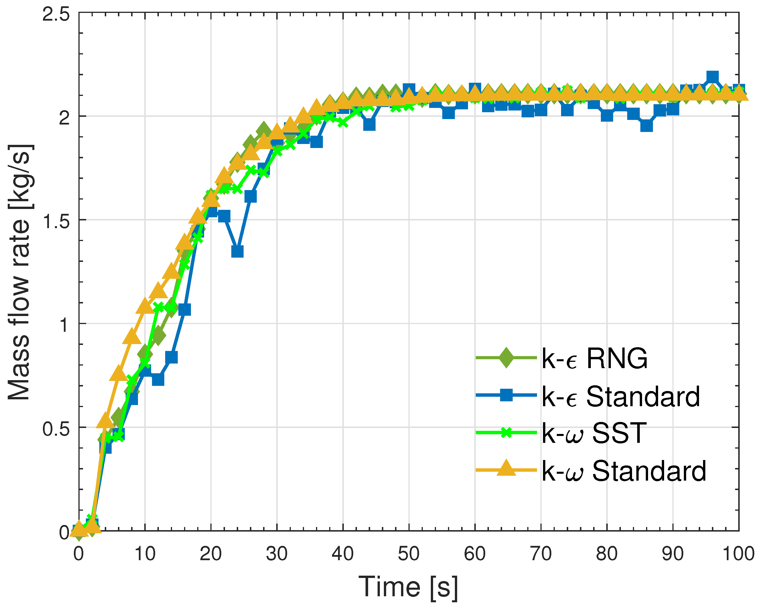
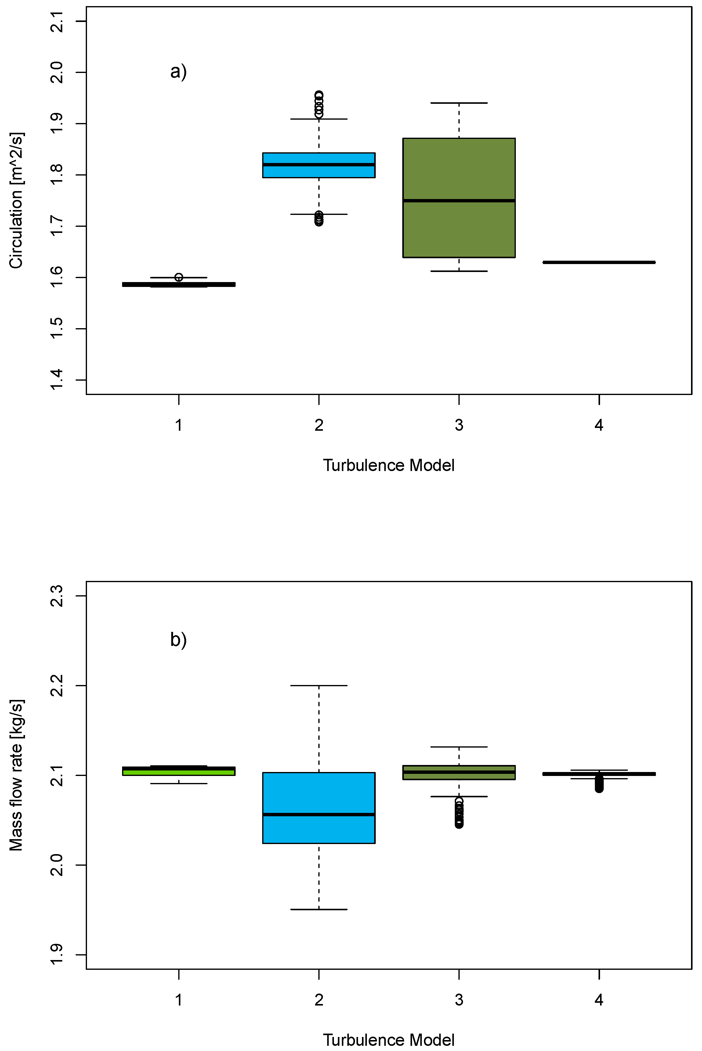
• It was observed that the behavior of the vortex circulation and the mass flow rate varied significantly between these models. This study revealed that the vortex circulation, which is a crucial parameter for understanding fluid dynamics, was dependent on the turbulence model used. While the k-$ϵ$ RNG and standard k-$\omega$ models exhibited similar circulation behaviors, including maintaining a relatively constant circulation value, the k-$ϵ$ standard model showed higher circulation values. In contrast, the k-$\omega$ SST model demonstrated an irregular circulation behavior, which fluctuated without evidence of stabilization during the analyzed time period. Similarly, the mass flow rate stabilization varied for each turbulence model. The k-$ϵ$ RNG, k-$\omega$ SST, and k-$\omega$ standard models stabilized around a value of 2.1 kg/s after 40 s. However, the standard k-$ϵ$ model exhibited fluctuations that ranged between 1.9 and 2.1 kg/s without being stabilized at the input mass flow rate value.
• Statistical analyses, including ANOVA and multiple comparison methods, confirmed the significant differences between the studied turbulence models for both the circulation and the mass flow rate. The obtained p-values indicate that the choice of the turbulence model significantly affected these variables, which reaffirmed the importance of the model selection in fluid dynamics simulations. Experimental tests were conducted to validate the numerical simulations.
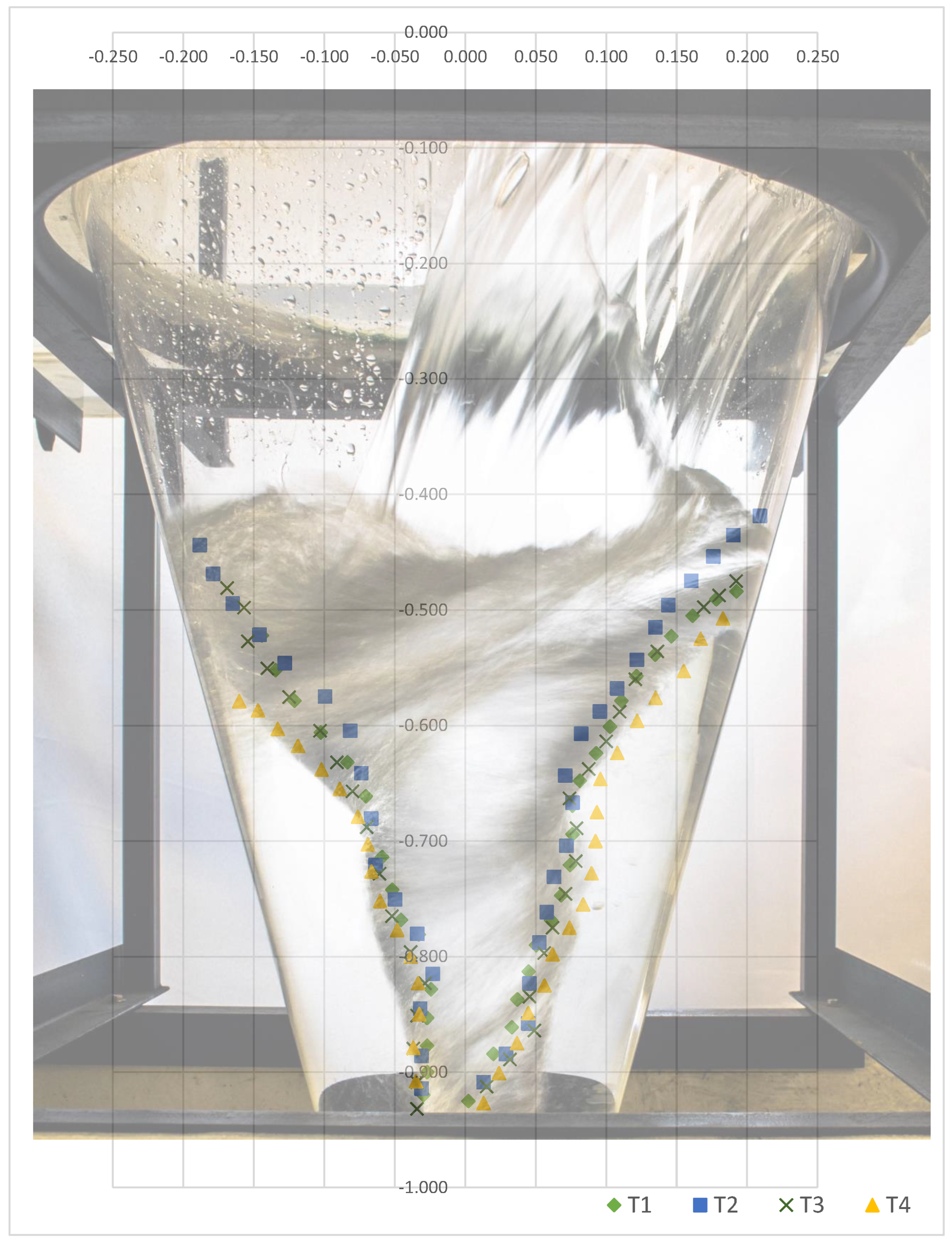
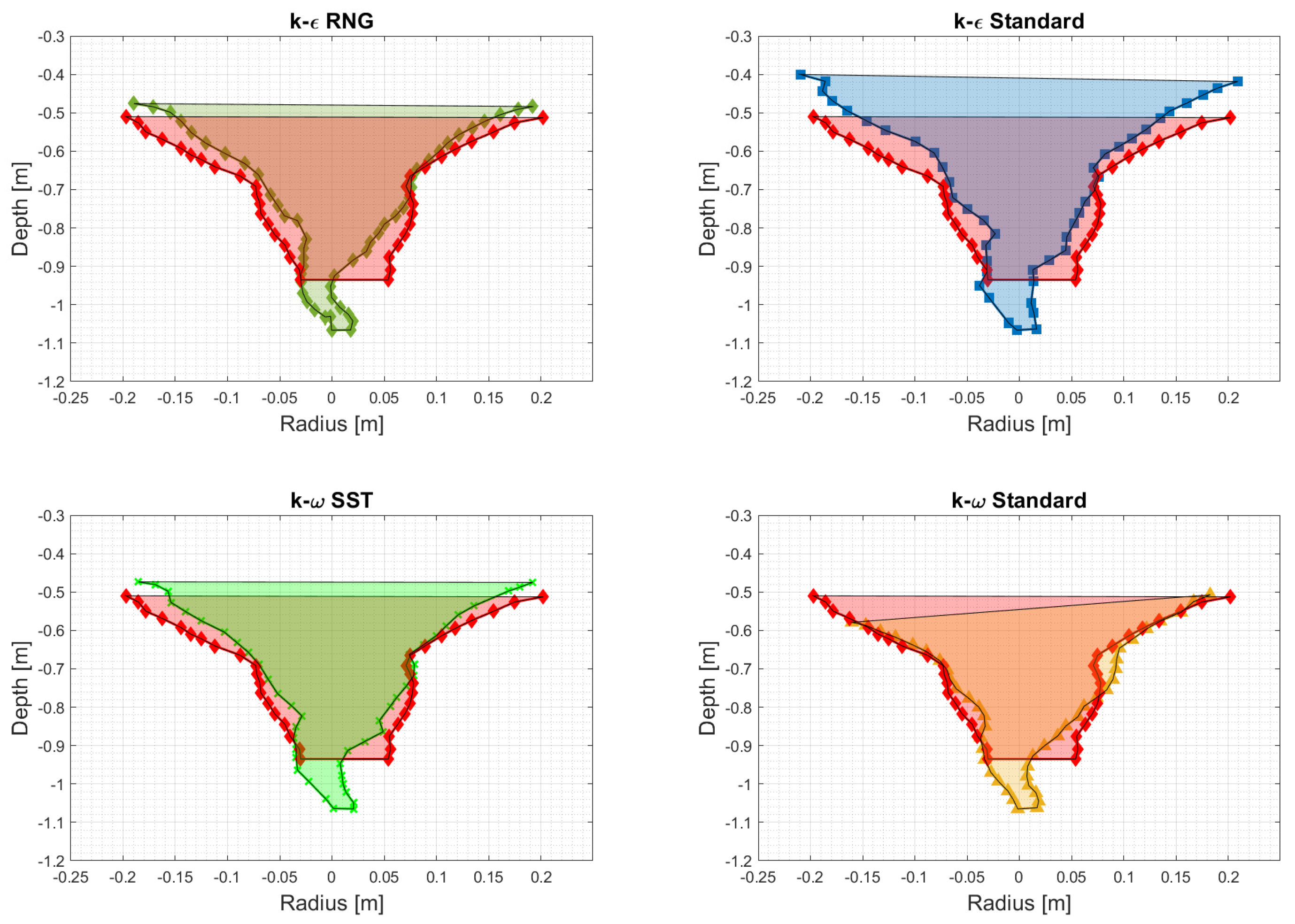
• By comparing the numerical vortex profiles with experimental results, it was confirmed that the k-$\omega$ SST model closely resembled the real vortex profile, followed by the k-$ϵ$ RNG model. This experimental validation provided additional support to the numerical findings and highlighted the effectiveness of the chosen turbulence models in capturing real-world phenomena.
• Based on the various analyses conducted, the k-$\omega$ SST model is recommended as the most appropriate turbulence model for this type of turbine. This model had a better ability to capture and predict the turbulence behavior in the studied system.

Future research into GWVHTs holds significant promise for enhancing their role as a renewable energy source:

• Continued efforts to optimize the turbine efficiency through advanced CFD simulations and experimental validations are crucial. This includes refining the turbulence models, such as further tuning the k-$\omega$ SST model, to improve the predictive accuracy under varying flow conditions. Optimization can also explore innovative designs and materials to enhance the turbine performance.
• Scaling up GWVHTs to larger capacities while maintaining efficiency is essential. Research could focus on modular designs or arrays of GWVHTs to harness energy from multiple low-head hydraulic sites effectively. Integration studies with existing water infrastructure, such as irrigation canals or urban drainage systems, could maximize energy recovery and sustainability benefits.
• Investigating the environmental impacts of GWVHT deployment by considering effects on aquatic ecosystems and local hydrology is critical. Research can explore mitigation strategies and sustainable practices to minimize the adverse effects and ensure long-term environmental stewardship. Additionally, assessing the socio-economic impacts of GWVHT projects on local communities, including job creation and energy access improvements, is essential for promoting equitable development.
• Conducting comprehensive techno-economic analyses to evaluate the cost-effectiveness of GWVHT installations compared with traditional hydropower and other renewable energy sources will play an important role. This includes assessing capital costs, operational and maintenance expenses, and the levelized cost of energy (LCOE). Such analyses can inform policy decisions and attract investment in GWVHT projects.

By addressing these aspects, GWVHTs can effectively be a reliable and environmentally friendly renewable energy source, thus playing a pivotal role in the global transition toward a sustainable energy future.

References

1. Velásquez, L.; Chica, E.; Posada, J. Advances in the Development of Gravitational Water Vortex Hydraulic Turbines. J. Eng. Sci. Technol. Rev. 2021, 14, 1–14. [Google Scholar] [CrossRef]
2. Looney, B. Statistical Review of World Energy, 2020; BP: London, UK, 2020. [Google Scholar]
3. Jogdand, O.K. Study on the effect of global warming and greenhouse gases on environmental system. In Green Chemistry and Sustainable Technology; Apple Academic Press: Cambridge, MA, USA, 2020; pp. 275–306. [Google Scholar]
4. Soeder, D.J. Fossil fuels and climate change. In Fracking and the Environment: A Scientific Assessment of the Environmental Risks from Hydraulic Fracturing and Fossil Fuels; Springer: Cham, Switzerland, 2021; pp. 155–185. [Google Scholar]
5. Singh, R.L.; Singh, P.K. Global environmental problems. In Principles and Applications of Environmental Biotechnology for a Sustainable Future; Springer: Cham, Switzerland, 2017; pp. 13–41. [Google Scholar]
6. Upadhyay, R.K. Markers for global climate change and its impact on social, biological and ecological systems: A review. Am. J. Clim. Chang. 2020, 9, 102270. [Google Scholar] [CrossRef]
7. Kushawaha, J.; Borra, S.; Kushawaha, A.K.; Singh, G.; Singh, P. Climate change and its impact on natural resources. In Water Conservation in the Era of Global Climate Change; Elsevier: Amsterdam, The Netherlands, 2021; pp. 333–346. [Google Scholar]
8. Halkos, G.E.; Gkampoura, E.C. Reviewing usage, potentials, and limitations of renewable energy sources. Energies 2020, 13, 2906. [Google Scholar] [CrossRef]
9. Holechek, J.L.; Geli, H.M.; Sawalhah, M.N.; Valdez, R. A global assessment: Can renewable energy replace fossil fuels by 2050? Sustainability 2022, 14, 4792. [Google Scholar] [CrossRef]
10. Rahman, A.; Farrok, O.; Haque, M.M. Environmental impact of renewable energy source based electrical power plants: Solar, wind, hydroelectric, biomass, geothermal, tidal, ocean, and osmotic. Renew. Sustain. Energy Rev. 2022, 161, 112279. [Google Scholar] [CrossRef]
11. Engeland, K.; Borga, M.; Creutin, J.D.; François, B.; Ramos, M.H.; Vidal, J.P. Space-time variability of climate variables and intermittent renewable electricity production—A review. Renew. Sustain. Energy Rev. 2017, 79, 600–617. [Google Scholar] [CrossRef]
12. Twidell, J. Renewable Energy Resources; Routledge: London, UK, 2021. [Google Scholar]
13. Timilsina, A.B.; Mulligan, S.; Bajracharya, T.R. Water vortex hydropower technology: A state-of-the-art review of developmental trends. Clean Technol. Environ. Policy 2018, 20, 1737–1760. [Google Scholar] [CrossRef]
14. Marian, G.; Sajin, T.; Florescu, I.; Nedelcu, D.; Ostahie, C.; Bîrsan, C. The concept and theoretical study of micro hydropower plant with gravitational vortex and turbine with rapidity steps. Bul. AGIR 2012, 3, 219–226. [Google Scholar]
15. Shabara, H.; Yaakob, O.; Ahmed, Y.M.; Elbatran, A.; Faddir, M.S. CFD validation for efficient gravitational vortex pool system. J. Teknol. 2015, 74. [Google Scholar] [CrossRef]
16. Sreerag, S.; Raveendran, C.; Jinshah, B. Effect of outlet diameter on the performance of gravitational vortex turbine with conical basin. Int. J. Sci. Eng. Res. 2016, 7, 457–463. [Google Scholar]
17. Velásquez, L.; Posada, A.; Chica, E. Optimization of the basin and inlet channel of a gravitational water vortex hydraulic turbine using the response surface methodology. Renew. Energy 2022, 187, 508–521. [Google Scholar] [CrossRef]
18. Sritram, P.; Treedet, W.; Suntivarakorn, R. Effect of turbine materials on power generation efficiency from free water vortex hydro power plant. IOP Conf. Ser. Mater. Sci. Eng. 2015, 103, 012018. [Google Scholar] [CrossRef]
19. Power, C.; McNabola, A.; Coughlan, P. A parametric experimental investigation of the operating conditions of gravitational vortex hydropower (GVHP). J. Clean Energy Technol. 2016, 4, 112–119. [Google Scholar] [CrossRef]
20. Wichian, P.; Suntivarakorn, R. The effects of turbine baffle plates on the efficiency of water free vortex turbines. Energy Procedia 2016, 100, 198–202. [Google Scholar] [CrossRef]
21. Betancour, J.; Romero-Menco, F.; Velásquez, L.; Rubio-Clemente, A.; Chica, E. Design and optimization of a runner for a gravitational vortex turbine using the response surface methodology and experimental tests. Renew. Energy 2023, 210, 306–320. [Google Scholar] [CrossRef]
22. Velásquez, L.; Romero-Menco, F.; Rubio-Clemente, A.; Posada, A.; Chica, E. Numerical optimization and experimental validation of the runner of a gravitational water vortex hydraulic turbine with a spiral inlet channel and a conical basin. Renew. Energy 2024, 220, 119676. [Google Scholar] [CrossRef]
23. Edirisinghe, D.S.; Yang, H.S.; Gunawardane, S.; Lee, Y.H. Enhancing the performance of gravitational water vortex turbine by flow simulation analysis. Renew. Energy 2022, 194, 163–180. [Google Scholar] [CrossRef]
24. Tamiri, F.; Yeo, E.; Ismail, M. Vortex profile analysis under different diffuser size for inlet channel of gravitational water vortex power plant. IOP Conf. Ser. Mater. Sci. Eng. 2022, 1217, 012014. [Google Scholar] [CrossRef]
25. Abel, A.; Tamiri, F.; Ismail, M.; Bohari, N. An Experience with Simulation Modeling for Vortex Flow in Micro Hydropower Systems. In Proceedings of the 2022 International Conference on Green Energy, Computing and Sustainable Technology (GECOST), Miri Sarawak, Malaysia, 26–28 October 2022; pp. 365–370. [Google Scholar]
26. Velásquez, L.; Posada, A.; Chica, E. Surrogate modeling method for multi-objective optimization of the inlet channel and the basin of a gravitational water vortex hydraulic turbine. Appl. Energy 2023, 330, 120357. [Google Scholar] [CrossRef]
27. Kamal, M.M.; Abbas, A.; Prasad, V.; Kumar, R. A numerical study on the performance characteristics of low head Francis turbine with different turbulence models. Mater. Today Proc. 2022, 49, 349–353. [Google Scholar] [CrossRef]
28. Mulligan, S. Experimental and Numerical Analysis of Three-Dimensional Free-Surface Turbulent Vortex Flows with Strong Circulation; Institute of Technology Sligo: Sligo, Ireland, 2015. [Google Scholar]
29. Holton, J.R. An introduction to dynamic meteorology. Am. J. Phys. 1973, 41, 752–754. [Google Scholar] [CrossRef]
30. Antuono, M.; Colagrossi, A.; Le Touzé, D.; Monaghan, J.J. Conservation of circulation in SPH for 2D free-surface flows. Int. J. Numer. Methods Fluids 2013, 72, 583–606. [Google Scholar] [CrossRef]
31. Cengel, Y.A. Fluid Mechanics; Tata McGraw-Hill Education: New York, NY, USA, 2010. [Google Scholar]
32. Zore, K.; Parkhi, G.; Sasanapuri, B.; Varghese, A. Ansys mosaic poly-hexcore mesh for high-lift aircraft configuration. In Proceedings of the 21th Annual CFD Symposium, Bangalore, India, 8–9 August 2019; pp. 1–11. [Google Scholar]
33. Rakowitz, M. Grid refinement study with a uhca wing-body configuration using richardson extrapolation and grid convergence index gci. In New Results in Numerical and Experimental Fluid Mechanics III; Springer: Berlin/Heidelberg, Germany, 2002; pp. 297–303. [Google Scholar]
34. Phillips, T.S.; Roy, C.J. Richardson extrapolation-based discretization uncertainty estimation for computational fluid dynamics. J. Fluids Eng. 2014, 136, 121401. [Google Scholar] [CrossRef]
35. Baker, N.; Kelly, G.; O’Sullivan, P.D. A grid convergence index study of mesh style effect on the accuracy of the numerical results for an indoor airflow profile. Int. J. Vent. 2020, 19, 300–314. [Google Scholar] [CrossRef]
36. Pope, S.B.; Pope, S.B. Turbulent Flows; Cambridge University Press: Cambridge, UK, 2000. [Google Scholar]
37. Maruzewski, P.; Hayashi, H.; Munch, C.; Yamaishi, K.; Hashii, T.; Mombelli, H.; Sugow, Y.; Avellan, F. Turbulence modeling for Francis turbine water passages simulation. IOP Conf. Ser. Earth Environ. Sci. 2010, 12, 012070. [Google Scholar] [CrossRef]
38. Dhakal, S.; Timilsina, A.B.; Dhakal, R.; Fuyal, D.; Bajracharya, T.R.; Pandit, H.P. Effect of dominant parameters for conical basin: Gravitational water vortex power plant. In Proceedings of the IOE Graduate Conference; Institute of Engineering, Tribhuvan University: Kathmandu, Nepal, 2014; p. 381. [Google Scholar]
39. Dhakal, S.; Timilsina, A.B.; Dhakal, R.; Fuyal, D.; Bajracharya, T.R.; Pandit, H.P.; Amatya, N.; Nakarmi, A.M. Comparison of cylindrical and conical basins with optimum position of runner: Gravitational water vortex power plant. Renew. Sustain. Energy Rev. 2015, 48, 662–669. [Google Scholar] [CrossRef]
40. Chattha, J.A.; Cheema, T.A.; Khan, N.H. Numerical investigation of basin geometries for vortex generation in a gravitational water vortex power plant. In Proceedings of the 2017 8th International Renewable Energy Congress (IREC), Amman, Jordan, 21–23 March 2017; pp. 1–5. [Google Scholar]
41. Nishi, Y.; Inagaki, T. Performance and flow field of a gravitation vortex type water turbine. Int. J. Rotating Mach. 2017, 2017, 2610508. [Google Scholar] [CrossRef]
42. Havaldar, S.; Gadekar, P.; Baviskar, S.; Jadhav, N.; Inamdar, S. Analyzing Geometries for Inlet Flow Channels to Gravitational Water Vortex Chamber. Int. J. Res. Eng. Appl. Manag. 2020, 5, 221–223. [Google Scholar]
43. ANSYS Inc. ANSYS Fluent 12.0 Theory Guide; ANSYS FLUENT Release; ANSYS Inc.: Canonsburg, PA, USA, 2009. [Google Scholar]
44. Chen, Q. Comparison of different k-ε models for indoor air flow computations. Numer. Heat Transf. Part B Fundam. 1995, 28, 353–369. [Google Scholar] [CrossRef]
45. Toapanta-Ramos, L.F.; Zapata-Cautillo, J.A.; Cholango-Gavilanes, A.I.; Quitiaquez, W.; Nieto-Londoño, C.; Zapata-Benabithe, Z. Estudio numérico y comparativo del efecto de turbulencia en codos y dobleces para distribución de agua sanitaria. Rev. Fac. De Ing. 2019, 28, 101–118. [Google Scholar] [CrossRef]
46. Monk, D.; Chadwick, E.A. Comparison of turbulence models effectiveness for a delta wing at low Reynolds numbers. In Proceedings of the 7th European Conference for Aeronautics and Space Sciences (EUCASS), Milan, Italy, 3–6 July 2017; Volume 1303. [Google Scholar]
47. Argyropoulos, C.D.; Markatos, N. Recent advances on the numerical modelling of turbulent flows. Appl. Math. Model. 2015, 39, 693–732. [Google Scholar] [CrossRef]
48. Notes, I.F. Introduction to CFD Analysis. Introductory FLUENT Training; ANSYS: Canonsburg, PA, USA, 2006. [Google Scholar]
49. Nasution, S.B.S.; Adanta, D. A Comparison of Openflume Turbine Designs with Specific Speeds (Ns) Based on Power and Discharge Function. J. Adv. Res. Fluid Mech. Therm. Sci. 2018, 51, 53–60. [Google Scholar]
50. R Core Team. R: A Language and Environment for Statistical Computing; R Foundation for Statistical Computing: Vienna, Austria, 2013. [Google Scholar]
51. Potter, K.; Hagen, H.; Kerren, A.; Dannenmann, P. Methods for presenting statistical information: The box plot. Vis. Large Unstructured Data Sets 2006, 4, 97–106. [Google Scholar]
52. Montgomery, D.C. Design and Analysis of Experiments; John Wiley & Sons: Hoboken, NJ, USA, 2017. [Google Scholar]
53. Rafter, J.A.; Abell, M.L.; Braselton, J.P. Multiple comparison methods for means. Siam Rev. 2002, 44, 259–278. [Google Scholar] [CrossRef]
54. Huttenlocher, D.P.; Klanderman, G.A.; Rucklidge, W.J. Comparing images using the Hausdorff distance. IEEE Trans. Pattern Anal. Mach. Intell. 1993, 15, 850–863. [Google Scholar] [CrossRef]
55. Taha, A.A.; Hanbury, A. An efficient algorithm for calculating the exact Hausdorff distance. IEEE Trans. Pattern Anal. Mach. Intell. 2015, 37, 2153–2163. [Google Scholar] [CrossRef] [PubMed]
56. Zhao, C.; Shi, W.; Deng, Y. A new Hausdorff distance for image matching. Pattern Recognit. Lett. 2005, 26, 581–586. [Google Scholar] [CrossRef]
57. Fischer, A.; Suen, C.Y.; Frinken, V.; Riesen, K.; Bunke, H. Approximation of graph edit distance based on Hausdorff matching. Pattern Recognit. 2015, 48, 331–343. [Google Scholar] [CrossRef]
58. Kumar, K.S.; Manigandan, T.; Chitra, D.; Murali, L. Object recognition using Hausdorff distance for multimedia applications. Multimed. Tools Appl. 2020, 79, 4099–4114. [Google Scholar] [CrossRef]
59. Kraft, D. Computing the Hausdorff distance of two sets from their distance functions. Int. J. Comput. Geom. Appl. 2020, 30, 19–49. [Google Scholar] [CrossRef]
60. Wang, S.; Tan, J.; Yu, Z. Comparison and experimental validation of turbulence models for an axial flow blood pump. J. Mech. Med. Biol. 2019, 19, 1940063. [Google Scholar] [CrossRef]
61. Muiruri, P.I.; Motsamai, O.S.; Ndeda, R. A comparative study of RANS-based turbulence models for an upscale wind turbine blade. SN Appl. Sci. 2019, 1, 237. [Google Scholar] [CrossRef]
62. Meana-Fernández, A.; Fernández Oro, J.M.; Argüelles Díaz, K.M.; Velarde-Suárez, S. Turbulence-model comparison for aerodynamic-performance prediction of a typical vertical-axis wind-turbine airfoil. Energies 2019, 12, 488. [Google Scholar] [CrossRef]
Figure 1. Dimensions of a gravitational water vortex hydraulic turbine (GWHT).
Energies 17 03543 g001
Figure 2. Hexcore mesh.
Energies 17 03543 g002
Figure 3. Boundary conditions.
Energies 17 03543 g003
Figure 4. Experimental setup.
Energies 17 03543 g004
Figure 5. Vortex circulation.
Energies 17 03543 g005
Figure 6. Mass flow rate.
Energies 17 03543 g006
Figure 7. Vortex profile from ANSYS Fluent: k- ϵ standard, k- ϵ RNG, k- ω standard, and k- ω SST models.
Energies 17 03543 g007
Figure 8. Vortex profile for a time of 100 s.
Energies 17 03543 g008
Figure 9. Angular velocity profile for a time of 100 s.
Energies 17 03543 g009
Figure 10. Box plots for the (a) vortex circulation and (b) mass flow rate. The numbers 1, 2, 3, and 4 correspond to the k- ϵ RNG model (T1), k- ϵ standard model (T2), k- ω SST model (T3), and k- ω standard model (T4).
Energies 17 03543 g010
Figure 11. Experimental vortex profile.
Energies 17 03543 g011
Figure 12. Comparison vortex profiles.
Energies 17 03543 g012
Figure 13. Air core area using k- ϵ standard, k- ϵ RNG, k- ω standard, and k- ω SST models.
Energies 17 03543 g013