
Investigation on Optimization Design of High-Thrust-Efficiency Pump Jet Based on Orthogonal Method


Abstract
1. Introduction
2. Pump Jet Design Method
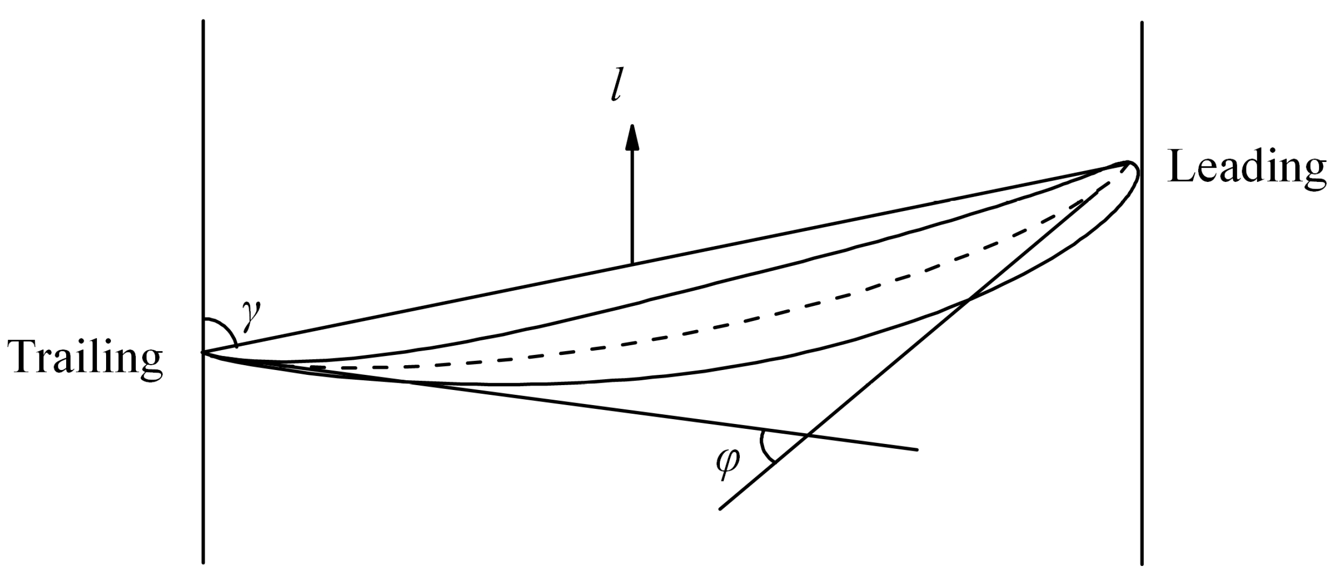
2.1. Blade Configuration Method
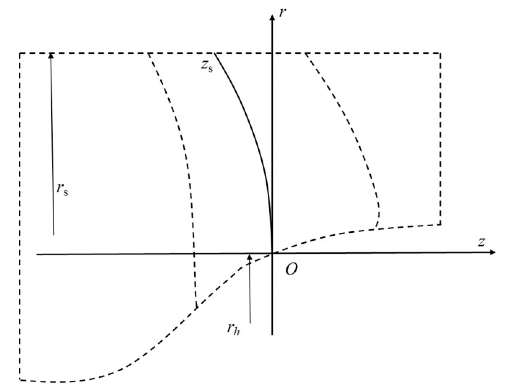
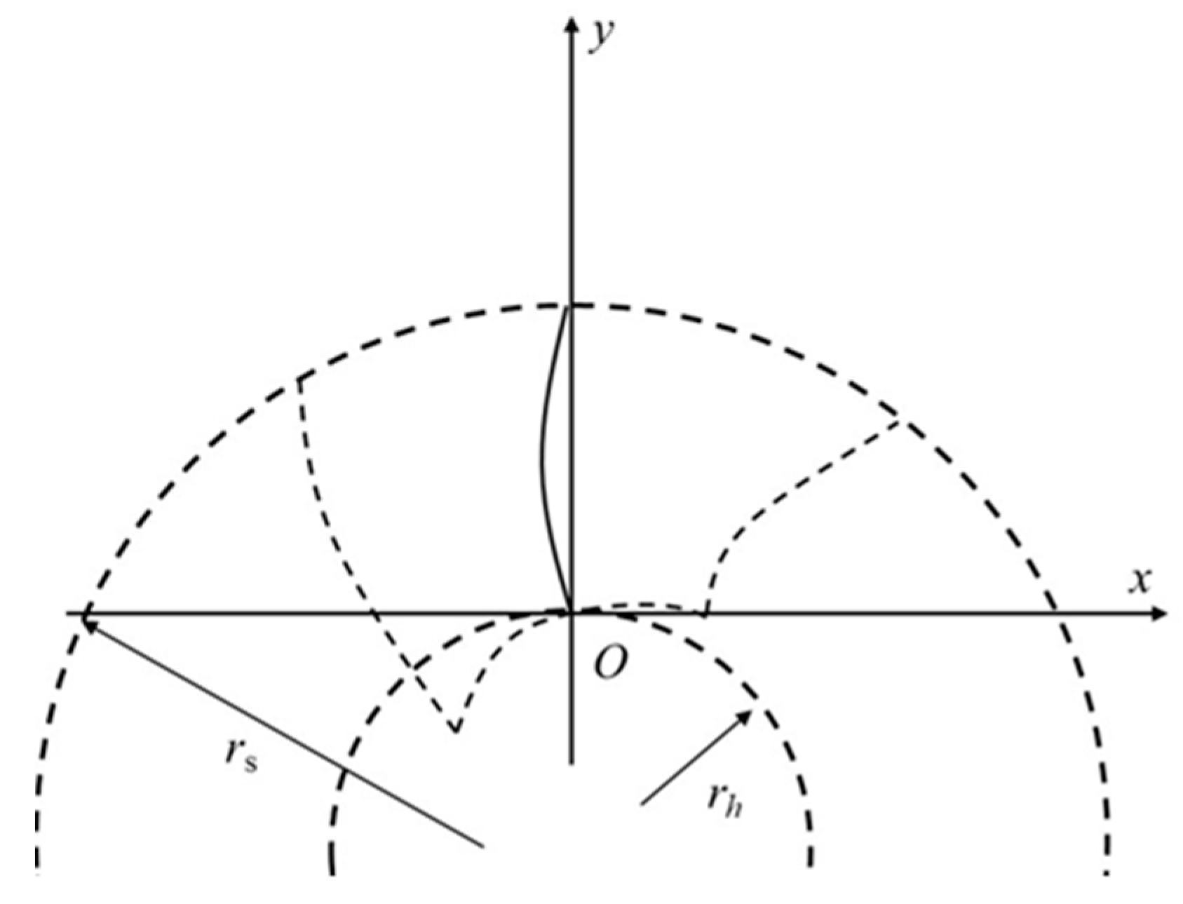
2.2. Blade Stacking Method
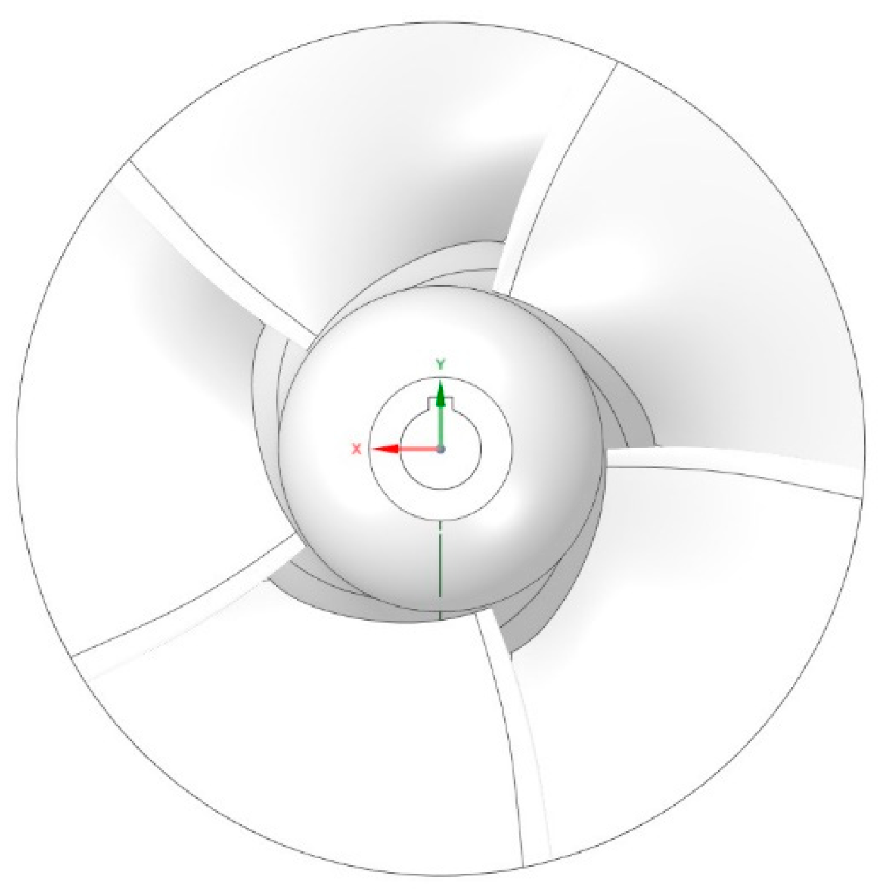
2.3. Design Results
3. Computational Domain and Numerical Method
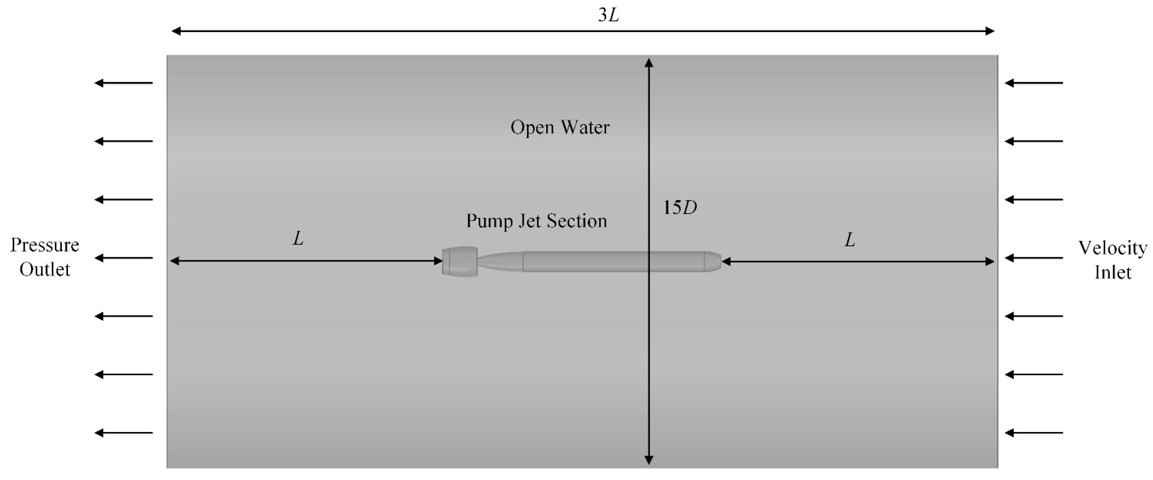
3.1. Computational Domain
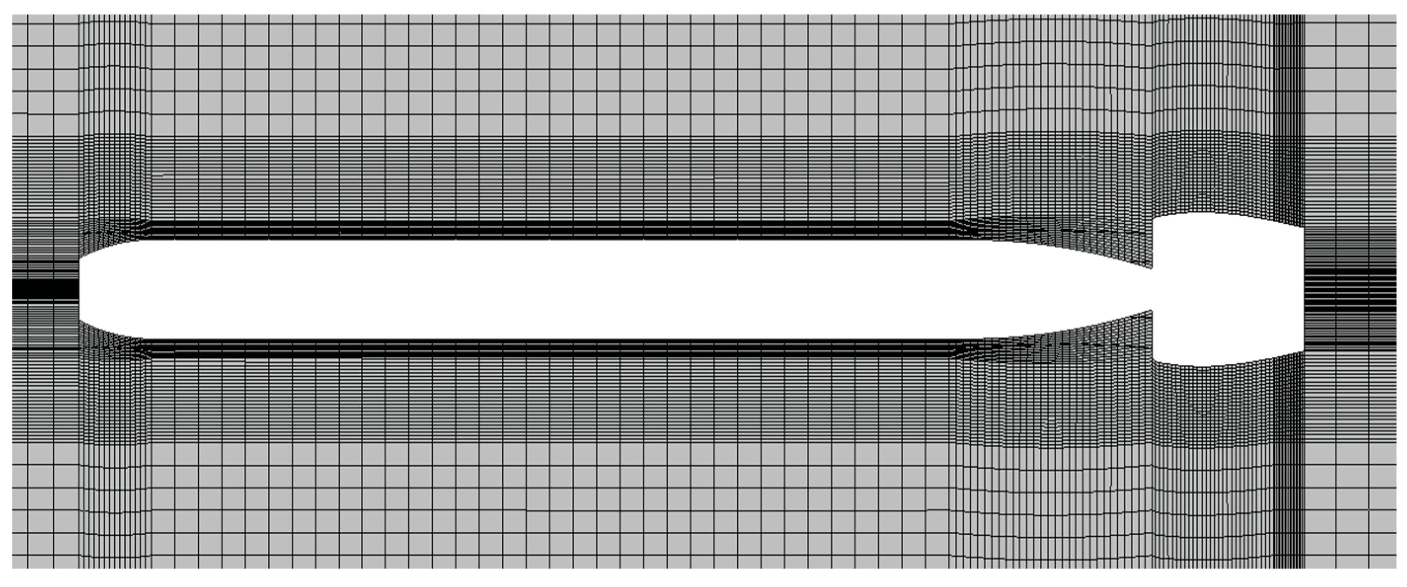
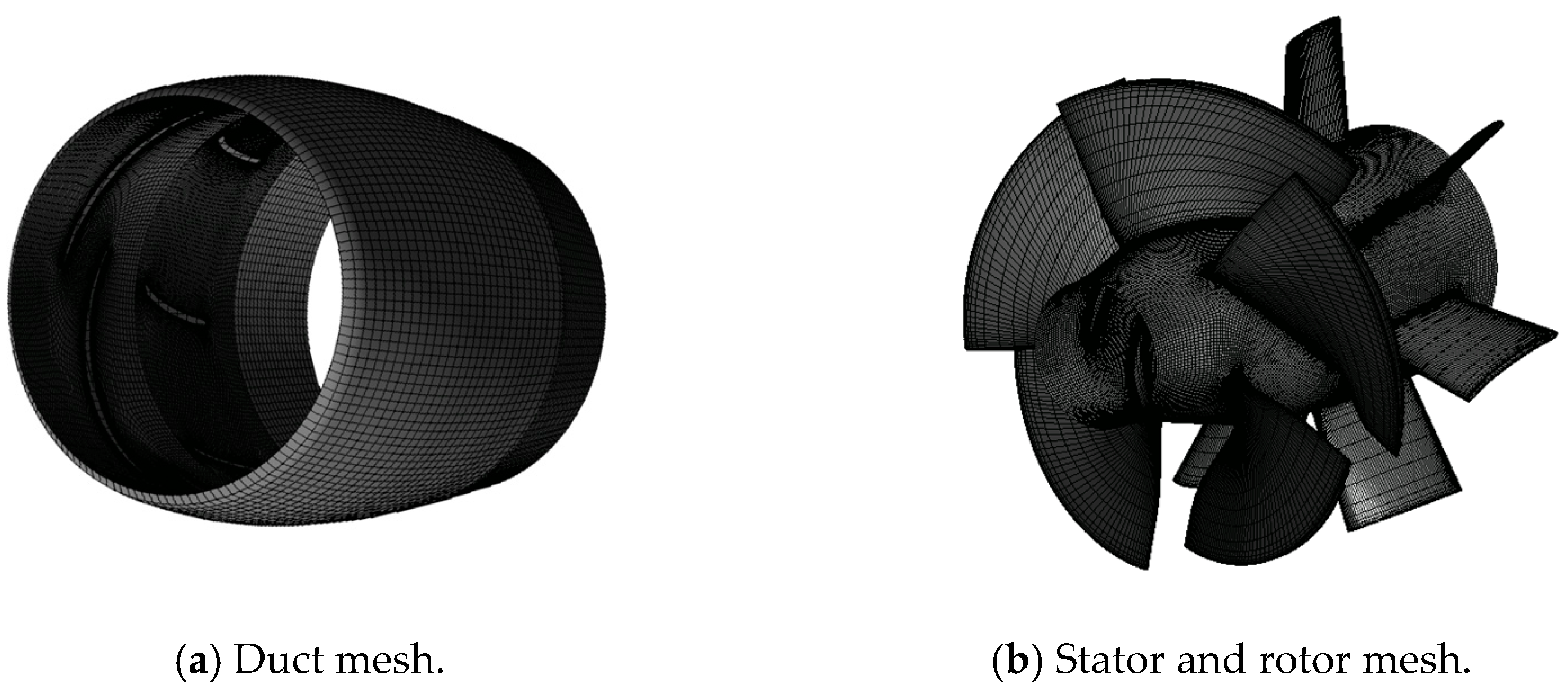
3.2. Computational Mesh
3.3. Mesh Independence Test
3.4. Numerical Method
4. Orthogonal Optimization
4.1. Airfoil Parameters
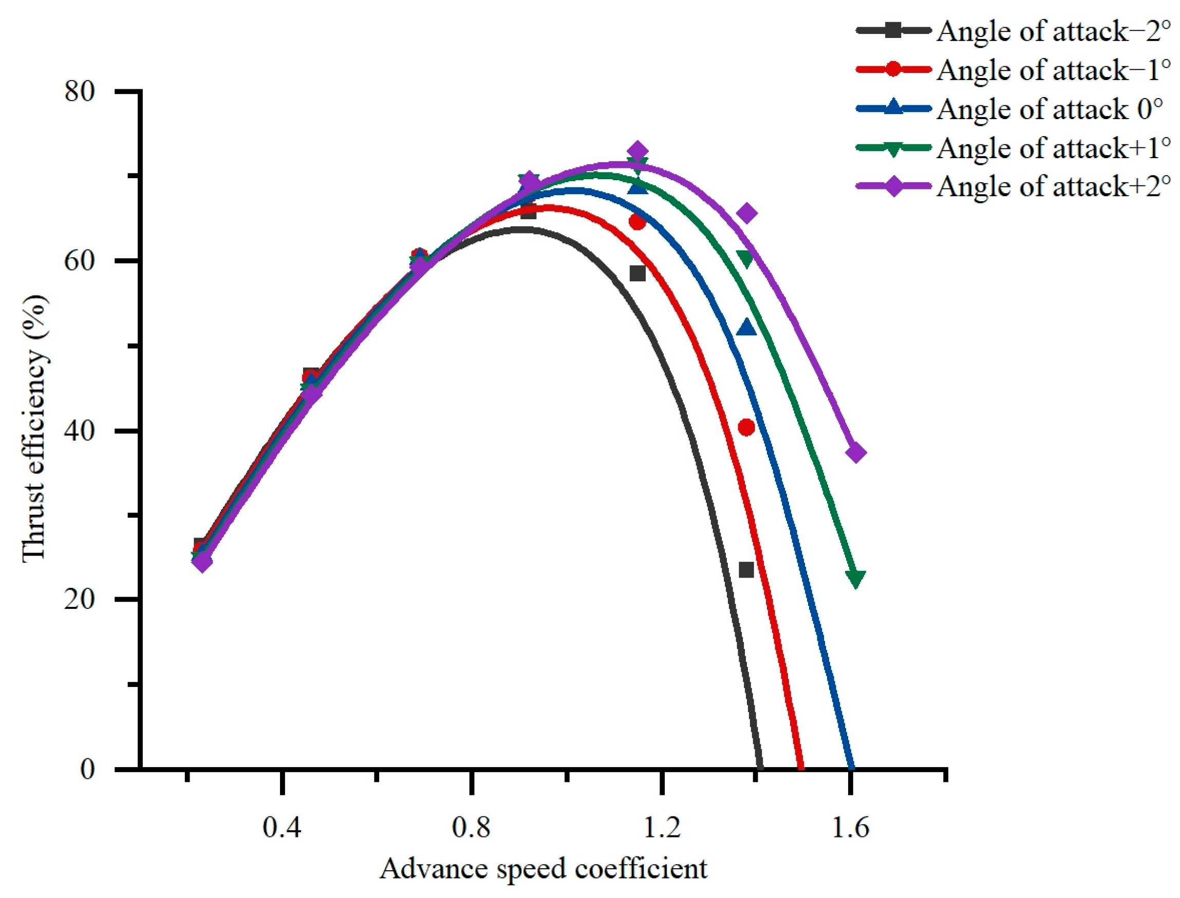
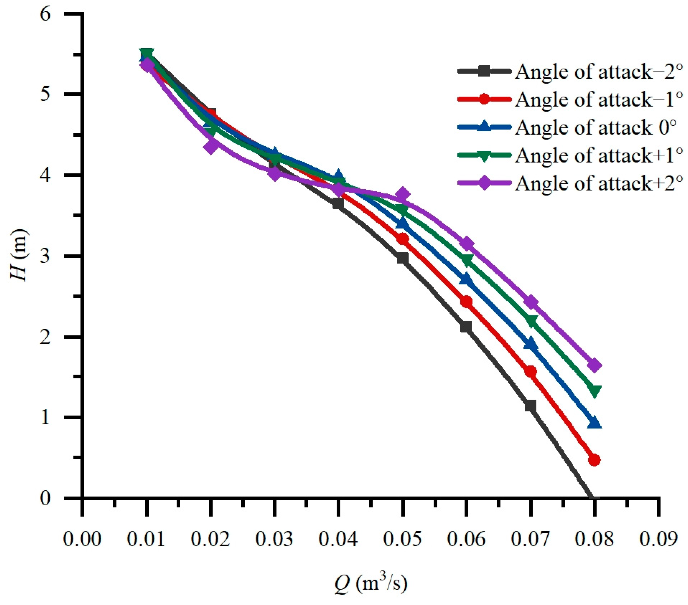
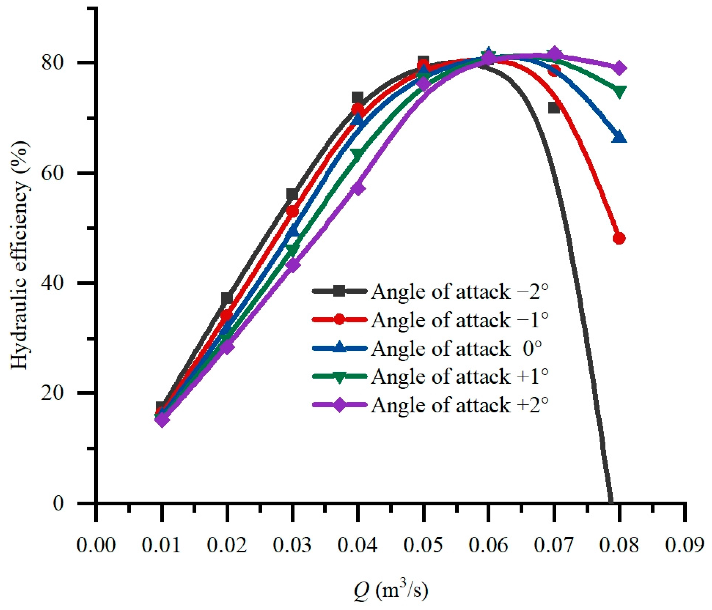
4.1.1. Angle of Attack
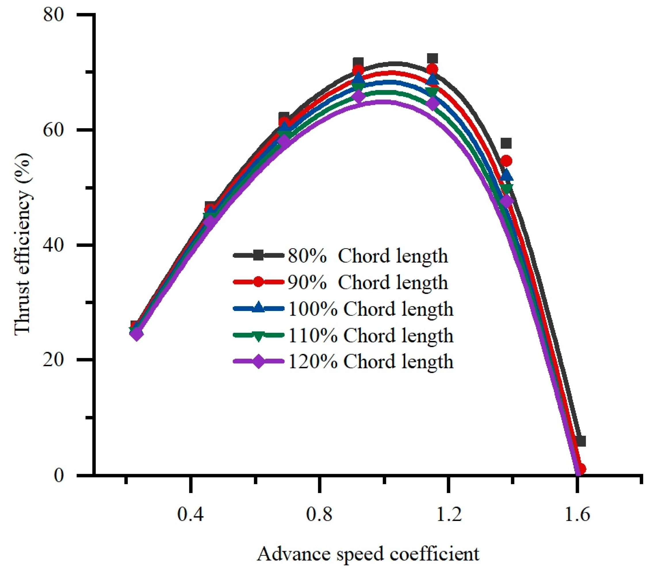
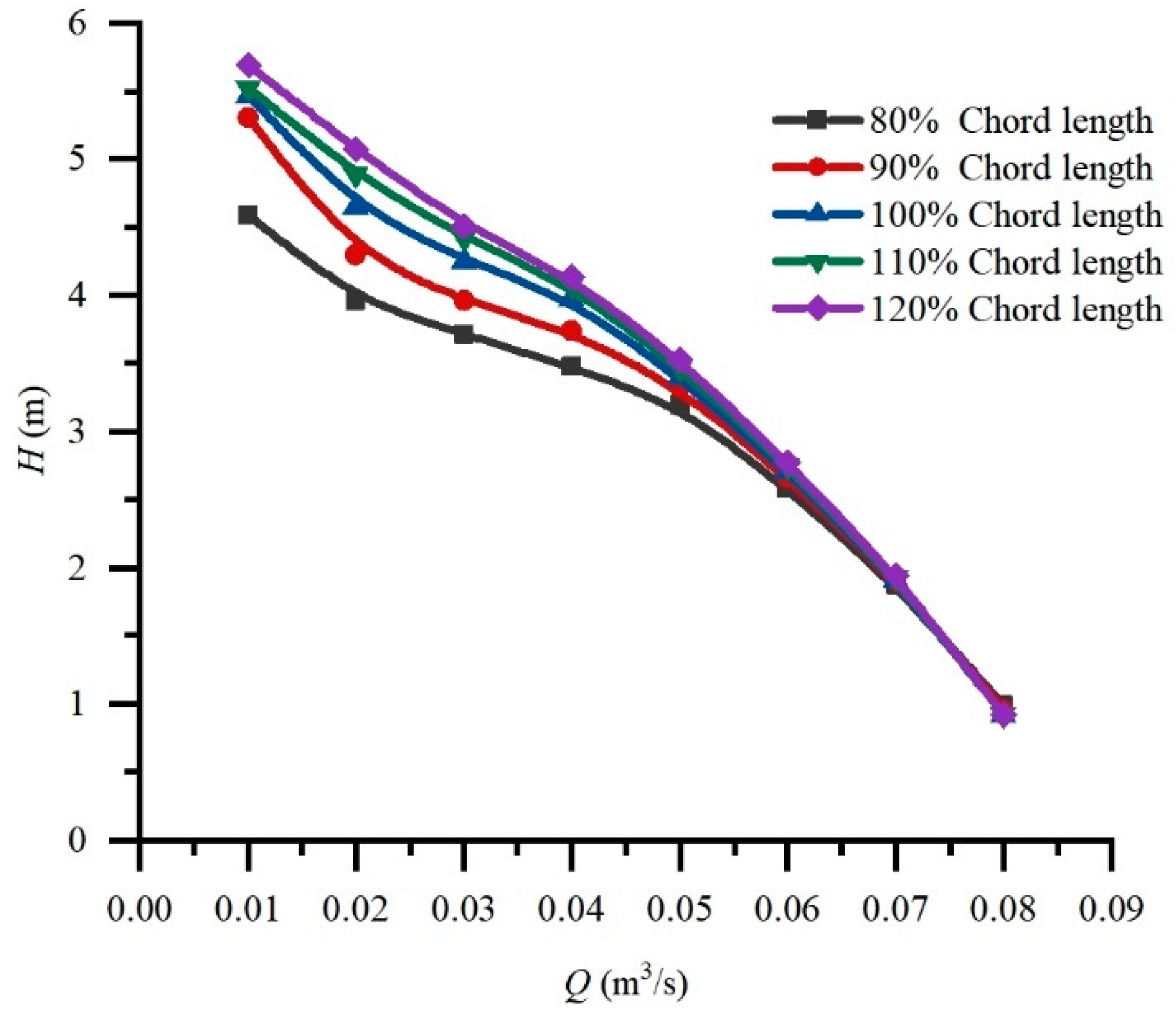
4.1.2. Chord Length
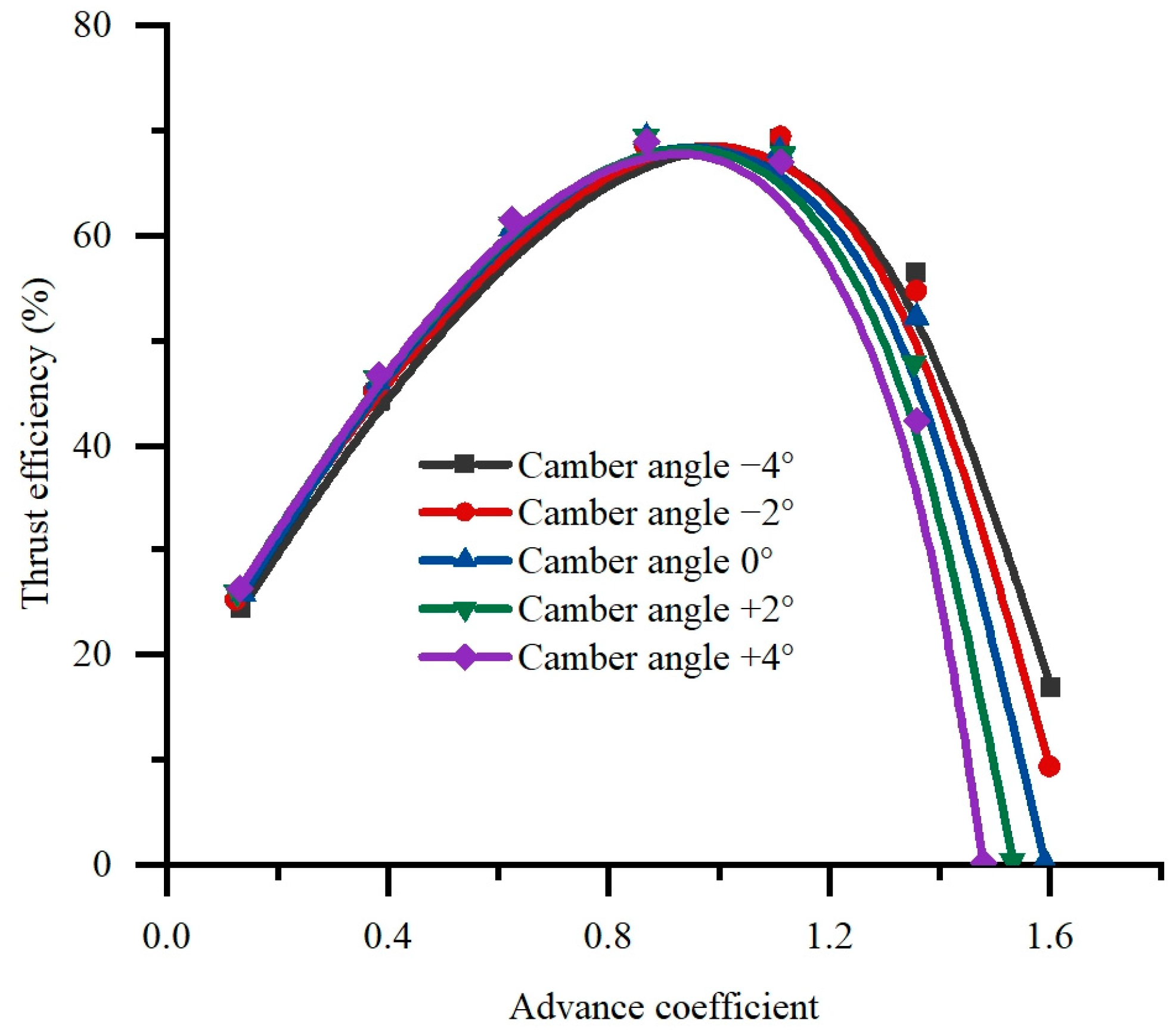
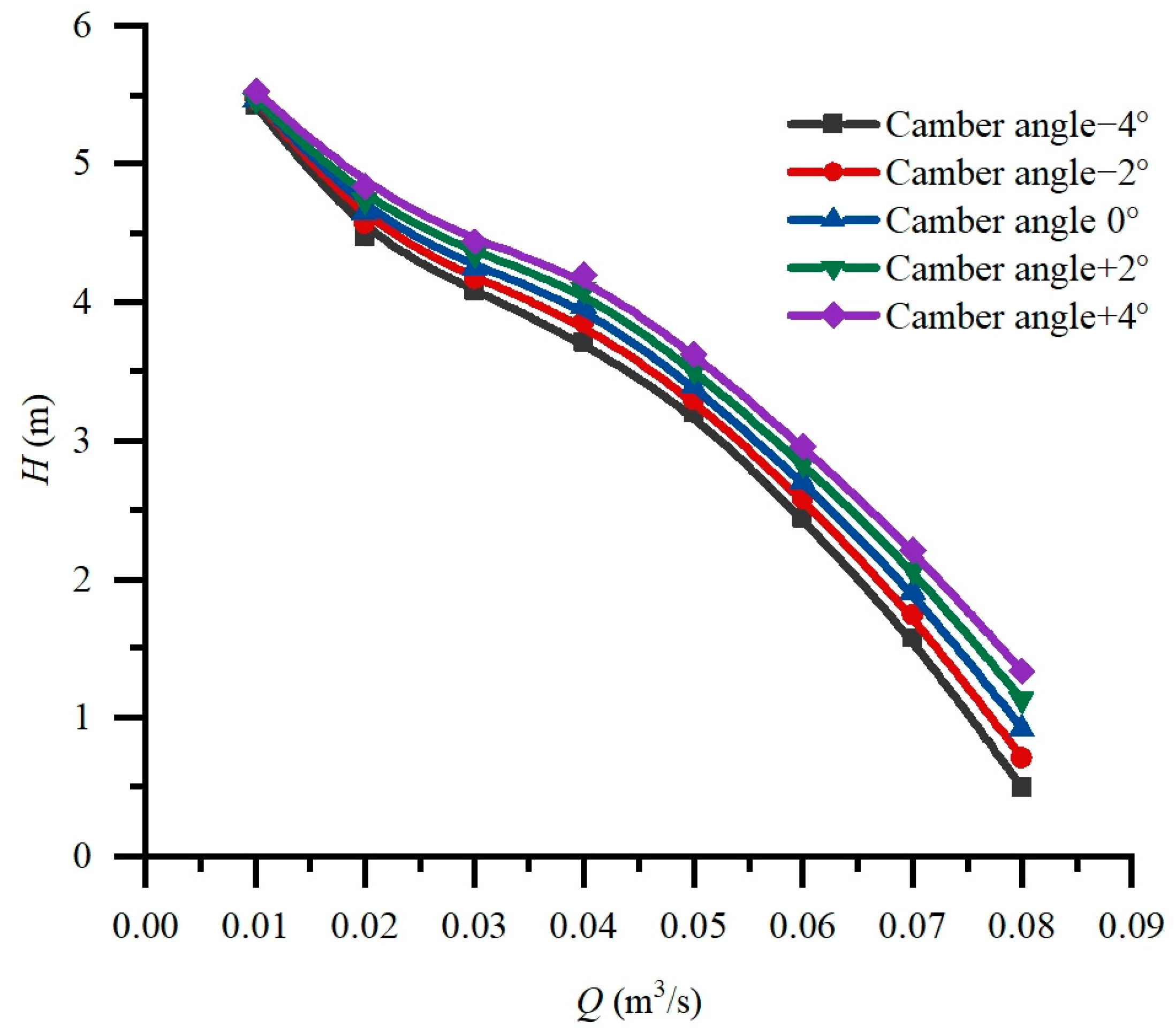
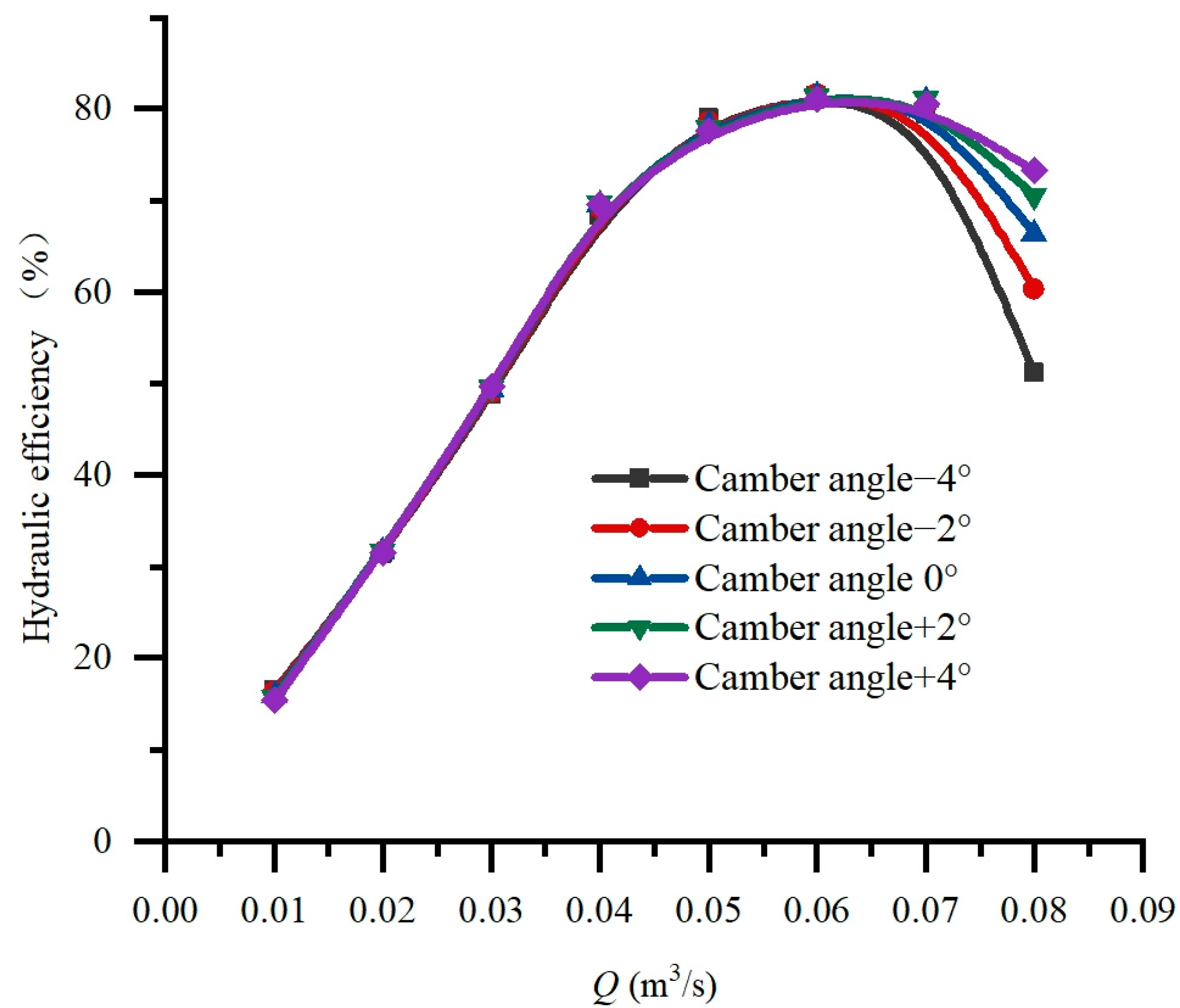
4.1.3. Camber Angle
4.2. Orthogonal Table
5. Results and Discussion
5.1. Orthogonal Analysis
5.2. Orthogonal Optimization
5.3. Flow Pattern Analysis
5.3.1. Simulation Result of Pressure
5.3.2. Simulation Result of Velocity
6. Conclusions
- (1)
- Increasing the angle of attack significantly improves the thrust performance and hydraulic performance of the pump, but it may cause abnormal flow at a small flow rate. The chord length has little effect on the thrust performance. The camber angle has little effect on the maximum thrust efficiency and hydraulic efficiency, but a larger camber angle is beneficial to large flow conditions and has a wider efficient working area.
- (2)
- According to a range analysis of the orthogonal method, as the angle of attack increases, the pump jet thrust efficiency increases; as the chord length increases, the thrust efficiency decreases; and, as the number of blades increases, the thrust efficiency decreases. The influence level of optimization parameters on pump jet thrust efficiency is sorted as follows: number of blades > angle of attack > chord length > camber angle.
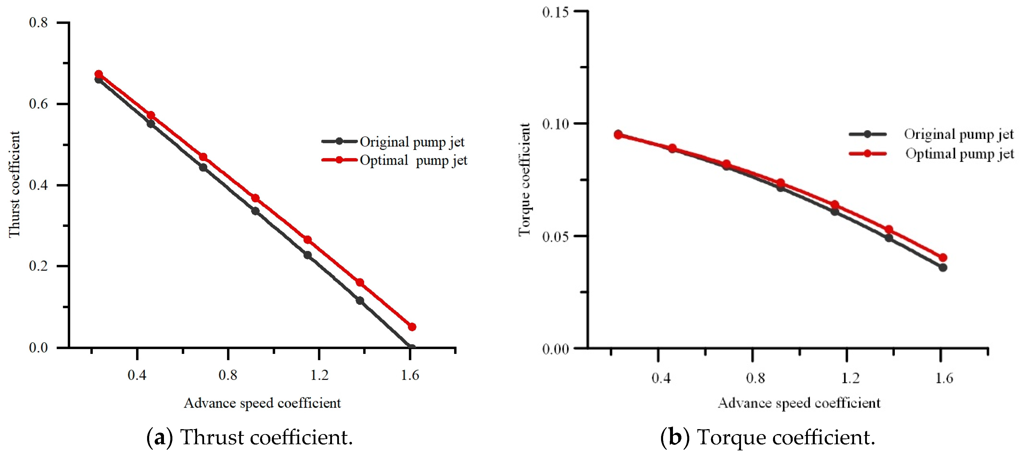
- (3)
- After the optimization, the thrust coefficient and thrust efficiency of the optimized pump jet are improved under different speed conditions, and the maximum thrust efficiency of the pump jet increased by 7.23%. The flow pattern in the optimal pump jet has been improved. The pressure gradient of the optimal pump jet becomes more fluent than that of original pump jet, which improves the energy performance.
Author Contributions
Funding
Data Availability Statement
Conflicts of Interest
References
- Gu, L.; Weng, K.; Wang, C. Review of torpedo pump-jet research. Collaborative Innovation and Forge ahead. In Proceedings of the Ninth Plenary Meeting of the Academic Committee of Ship Mechanics, Manchester, UK, 25–28 July 2018; pp. 125–139. [Google Scholar]
- Mccormic, B.; Eisenhuth, J. Design and performance of propellers and pump jets for underwater propulsion. AIAA J. 1963, 1, 2348–2354. [Google Scholar] [CrossRef]
- Peng, Y.; Wang, Y.; Liu, C.; Li, W. Comparison of hydrodynamic performance of front-mounted and rear-mounted stator pump-jet thrusters. J. Harbin Eng. Univ. 2019, 40, 132–140. [Google Scholar]
- Goldstein, S. On the vortex of screw propellers. Proc. R. Soc. 1929, 123, 440–465. [Google Scholar]
- Lerbs, H. Moderately loaded propellers with finite number blades and an arbitrary distribution of circulations. Trans SNAME 1952, 60, 73–123. [Google Scholar]
- Kawada, S. Induced velocity by helical vortices. J. Aeronaut. Sci. 1936, 3, 86–87. [Google Scholar] [CrossRef]
- Liang, J.; Lu, L.; Xu, L.; Chen, W.; Wang, G. Effect of the water velocity circulation at the outlet of the guide vane of the axial flow pump device on the hydraulic loss of the outlet channel. Chin. J. Agric. Eng. 2012, 28, 55–60. [Google Scholar]
- Zhang, D.; Li, T.; Shi, W.; Zhang, H.; Zhang, G. Experimental study on axial velocity and circulation volume at the outlet of axial flow pump impeller. Chin. J. Agric. Eng. 2012, 28, 73–77. [Google Scholar]
- Xie, R. Research on Hydraulic Characteristics of Axial Flow Pump under Small Flow Conditions. Ph.D. Thesis, Yangzhou University, Yangzhou, China, 2016. [Google Scholar]
- Song, Y.; Chen, H.; Li, Y.; Chen, F. Effect of Coanda surface shape on circulation control turbine blade performance. J. Eng. Thermo Phys. 2012, 33, 43–46. [Google Scholar]
- Mu, A.; Yang, W.; Zhang, M.; Liu, H.; Zhang, Y. Design and research of Magnus wind turbine combined rotating circular wing based on the influence of toroidal field. J. Sol. Energy 2015, 36, 2460–2466. [Google Scholar]
- Xie, F.; Xuan, R.; Sheng, G.; Wang, C. Flow characteristics of accelerating pump in hydraulic-type wind power generation system under different wind speeds. Int. J. Adv. Manuf. Technol. 2017, 92, 189–196. [Google Scholar] [CrossRef]
- Zhang, N.; Liu, X.; Gao, B.; Wang, X.; Xia, B. Effects of modifying the blade trailing edge profile on unsteady pressure pulsations and flow structures in a centrifugal pump. Int. J. Heat Fluid Flow 2019, 75, 227–238. [Google Scholar] [CrossRef]
- Zhang, N.; Yang, M.; Gao, B.; Li, Z.; Ni, D. Investigation of Rotor-Stator Interaction and Flow Unsteadiness in a Low Specific Speed Centrifugal Pump. Stroj. Vestn. J. Mech. Eng. 2016, 62, 21–31. [Google Scholar] [CrossRef]
- Han, S. Optimization Design and Experimental Research of High Power Density Axial Flow Pump. Ph.D. Thesis, Tsinghua University, Beijing, China, 2022. [Google Scholar]
- Cox, G. Corrections to the camber of constant pitch propeller. Trans. RINA 1961, 103, 227–243. [Google Scholar]
- Greeley, D. Marine Propeller Blade Tip Flows. Ph.D. Thesis, Department of Mechanical Engineering, MIT, Cambridge, MA, USA, 1982. [Google Scholar]
- Wang, G.; Yang, J. Estimating propeller cavitation using the lifting surface method. J. Shanghai Jiao Tong Univ. 1993, 9–18. [Google Scholar]
- Wang, G.; Yang, C. Theoretical design method of cavitation propeller lifting surface. Ship Mech. 2002, 6, 11–17. [Google Scholar]
- Dong, S. Refined treatment of the theoretical boundary value problem of propeller lifting surface. Ship Mech. 2004, 8, 1–15. [Google Scholar]
- Tan, T.; Xiong, Y. Propeller lifting surface design based on B-spline. J. Nav. Eng. Univ. 2005, 17, 37–42. [Google Scholar]
- Lu, L.; Pan, G.; Sahoo, P.K. CFD prediction and simulation of a pump jet propulsor. Int. J. Nav. Archit. Ocean. Eng. 2016, 8, 110–116. [Google Scholar]
- Lu, L.; Gao, Y.; Li, Q.; Du, L. Numerical investigations of tip clearance flow characteristics of a pump jet propulsor. Int. J. Nav. Archit. Ocean. Eng. 2018, 10, 307–317. [Google Scholar] [CrossRef]
- Ahn, S.; Kwon, O. Numerical investigation of a pump-jet with ring rotor using an unstructured mesh technique. J. Mech. Sci. Technol. 2015, 29, 2897–2904. [Google Scholar] [CrossRef]
- Bontempo, R.; Cardone, M.; Manna, M. Performance analysis of ducted marine propellers. Part I—Decelerating duct. Appl. Ocean. Res. 2016, 58, 322–330. [Google Scholar] [CrossRef]
- Bontempo, R.; Manna, M. Performance analysis of ducted marine propellers. Part II—Accelerating duct. Appl. Ocean. Res. 2018, 75, 153–164. [Google Scholar] [CrossRef]
- Xu, Y.; Tan, L.; Cao, S.; Qu, W. Multiparameter and multiobjective optimization design of centrifugal pump based on orthogonal method. Proc. Inst. Mech. Eng. Part C J. Mech. Eng. Sci. 2017, 231, 2569–2579. [Google Scholar] [CrossRef]
- Liu, M.; Tan, L.; Cao, S. Design method of controllable blade angle and orthogonal optimization of pressure rise for a multiphase pump. Energies 2018, 11, 1048. [Google Scholar] [CrossRef]
- Yuan, J.; Fan, M.; Giovanni, P.; Lu, R.; Li, Y.J.; Fu, Y.X. Research on orthogonal optimization design of high specific speed axial flow pump. Vib. Impact 2018, 37, 115–121. [Google Scholar]
- Zheng, Y.; Sun, A.; Yang, C.; Jiang, W. Multi-objective optimization orthogonal test of axial flow pump. J. Agric. Mach. 2017, 48, 129–136. [Google Scholar]


| Design Parameter | Value |
|---|---|
| Speed Vs/kn | 8 |
| Thrust T/N | 120 |
| Speed n/(r/min) | 1450 |
| Flow Q/(m3/s) | 0.06 |
| Head H/m | 2.7 |
| Impeller diameter D/mm | 180 |
| Specific speed ns | 615 |
| Number | Mesh1 | Mesh2 | Mesh3 | Mesh4 | Mesh5 | Mesh6 |
|---|---|---|---|---|---|---|
| Open water | 722,208 | 995,483 | 1,333,768 | 1,947,248 | 2,931,808 | 3,884,328 |
| Pump jet area | 1,727,778 | 1,727,778 | 1,727,778 | 1,727,778 | 1,727,778 | 1,727,778 |
| Relative resistance | 1 | 0.985812 | 0.975463 | 0.961081 | 0.951509 | 0.948059 |
| Number | Mesh7 | Mesh8 | Mesh9 | Mesh10 | Mesh11 |
|---|---|---|---|---|---|
| Open water | 2,931,808 | 2,931,808 | 2,931,808 | 2,931,808 | 2,931,808 |
| Rotor | 238,170 | 441,980 | 751,920 | 1,298,100 | 1,464,960 |
| Stator | 331,722 | 667,436 | 1,005,368 | 1,698,060 | 1,994,272 |
| Pump jet area | 569,892 | 1,109,416 | 1,757,288 | 2,996,160 | 3,459,232 |
| Relative resistance | 1 | 1.017042 | 1.028312 | 1.030201 | 1.030866 |
| Level | Angle of Attack/° (A) | Chord Length (B) | Camber Angle/° (C) | Number of Blades (D) |
|---|---|---|---|---|
| 1 | −1 | 0.8 L | −2 | 4 |
| 2 | 0 | 0.9 L | 0 | 5 |
| 3 | 1 | L | 2 | 6 |
| Individual No. | Factor | |||
|---|---|---|---|---|
| A/° | B | C/° | D | |
| 1 | −1 | 0.8 L | −2 | 4 |
| 2 | −1 | 0.9 L | 0 | 5 |
| 3 | −1 | L | 2 | 6 |
| 4 | 0 | 0.8 L | 0 | 6 |
| 5 | 0 | 0.9 L | 2 | 4 |
| 6 | 0 | L | 2 | 5 |
| 7 | 1 | 0.8 L | 2 | 5 |
| 8 | 1 | 0.9 L | −2 | 6 |
| 9 | 1 | L | 0 | 4 |
| Individual No. | Thrust Efficiency/% | Flow/m3/s | Head/m | Hydraulic Efficiency/% |
|---|---|---|---|---|
| 1 | 0.731 | 0.06 | 2.05 | 0.826 |
| 2 | 0.698 | 0.06 | 2.47 | 0.830 |
| 3 | 0.631 | 0.06 | 2.65 | 0.800 |
| 4 | 0.693 | 0.06 | 2.71 | 0.816 |
| 5 | 0.750 | 0.06 | 2.62 | 0.826 |
| 6 | 0.692 | 0.06 | 2.62 | 0.818 |
| 7 | 0.752 | 0.06 | 2.94 | 0.818 |
| 8 | 0.689 | 0.06 | 2.87 | 0.810 |
| 9 | 0.744 | 0.06 | 2.79 | 0.826 |
| Thrust Efficiency | Factor | |||
| A | B | C | D | |
| 0.6865 | 0.7252 | 0.7037 | 0.7417 | |
| 0.7116 | 0.7123 | 0.7116 | 0.7141 | |
| 0.7284 | 0.689 | 0.7112 | 0.6706 | |
| R | 0.0419 | 0.0362 | 0.0079 | 0.0711 |
| Order | 2 | 3 | 4 | 1 |
Disclaimer/Publisher’s Note: The statements, opinions and data contained in all publications are solely those of the individual author(s) and contributor(s) and not of MDPI and/or the editor(s). MDPI and/or the editor(s) disclaim responsibility for any injury to people or property resulting from any ideas, methods, instructions or products referred to in the content. |
© 2024 by the authors. Licensee MDPI, Basel, Switzerland. This article is an open access article distributed under the terms and conditions of the Creative Commons Attribution (CC BY) license (https://creativecommons.org/licenses/by/4.0/).
Share and Cite
Zhang, X.; Dai, Z.; Yang, D.; Fan, H. Investigation on Optimization Design of High-Thrust-Efficiency Pump Jet Based on Orthogonal Method. Energies 2024, 17, 3551. https://doi.org/10.3390/en17143551
Zhang X, Dai Z, Yang D, Fan H. Investigation on Optimization Design of High-Thrust-Efficiency Pump Jet Based on Orthogonal Method. Energies. 2024; 17(14):3551. https://doi.org/10.3390/en17143551
Chicago/Turabian StyleZhang, Xiaojun, Zhenxing Dai, Dangguo Yang, and Honggang Fan. 2024. "Investigation on Optimization Design of High-Thrust-Efficiency Pump Jet Based on Orthogonal Method" Energies 17, no. 14: 3551. https://doi.org/10.3390/en17143551
APA StyleZhang, X., Dai, Z., Yang, D., & Fan, H. (2024). Investigation on Optimization Design of High-Thrust-Efficiency Pump Jet Based on Orthogonal Method. Energies, 17(14), 3551. https://doi.org/10.3390/en17143551