Modeling and CFD Simulation of Macroalgae Motion within Aerated Tanks: Assessment of Light-Dark Cycle Period

Abstract

Computational techniques can be applied to numerically assess key parameters influencing the biotechnological process to better predict the essential features governing macroalgae growth and nutrient removal in aerated tanks, e.g., integrated into multitrophic aquaculture systems. Recent advances in computational hardware and software, such as the discrete element method (DEM) coupled with computational fluid dynamics (CFDs) codes, have enabled flow simulations in biotechnological systems. Here, we perform CFD-DEM simulations of macroalgae motion within aerated tanks to assess the light–dark cycle period as one of the most critical abiotic conditions governing the growth of photosynthetic organisms. This proof-of-concept study, which deals with the challenging problem of the fluid–structure interaction in aerated (bubbled) tanks with a highly flexible solid phase, includes a set of detailed 2D CFD simulations for two types of settings differing in the presence or absence of an inner cylinder assembly. Consequently, corresponding regression models for the cycle period are derived, and the initial hypothesis of the assembly’s beneficial role is confirmed. Eventually, the CFD results are verified using an image processing technique on the laboratory scale tank with Ulva sp. and specific 3D CFD-DEM simulations.

1. Introduction

The mathematical modeling and optimization of biotechnological production systems, such as integrated multitrophic aquaculture (IMTA) [1,2,3], are challenging due to the inherent complexity of the biotic and abiotic conditions influencing the system’s performance. For instance, predictive mechanistic models, describing the role of multiphase flow dynamics and/or light regimes in tanks with specific microalgae strains [4,5,6], are scarce; this is especially true for macroalgae (also called seaweed). This is why some researchers, in similar cases, prefer probabilistic models that encode a parsimonious representation, claiming that models are more efficient for bioprocess description and optimization [7]. The drawback of such models is that there are no data for designing and optimizing new production systems. Therefore, this work aims to develop mechanistic models describing macroalgae motion in aerated tanks (an important part of inland IMTA systems) in silico, to validate them using small-scale laboratory equipment, and to eventually provide the missing data for further steps involving either the optimization of equipment design or process control.

Let us underline that among inland IMTA techniques, the integration of fish and macroalgae cultures in recirculating aquaculture systems (RASs) is currently one of the most promising lines of action to reduce the pressure on open-sea fishing and the use of terrestrial and inland water resources [8,9,10,11]. However, besides the lack of reliable mathematical models for further process control and optimization, there are two limiting factors or drawbacks in the case of macroalgae cultivation integrated with RAS, e.g., Ulva sp., which are the large area required and the energy costs. Reducing the area required for seaweed cultivation in tanks implies an increase in yield, which can be achieved using a proper combination of stocking densities and the light regime that macroalgal culture undergoes [12]. Concerning energy costs, the major energy sink in land-based macroalgae culture systems is designed to tumble (mix) macroalgae (either through bottom aeration or a water jet array). Tumbling seaweed in the tanks promotes better nutrient and gas exchange between the culture medium and macroalgae (because the thickness of the boundary layer decreases when the mixing intensity increases) [13] and may enhance the photosynthetic efficiency due to a higher light–dark cycle frequency, e.g., [14,15,16,17]. While in the above-mentioned studies, the intermittent irradiance was provided by the intermittent lighting of the light source, here, the essential components are the existence of the irradiance gradient in the tank’s vertical axis and the cyclic motion of the seaweed fronds in the same direction. Therefore, hydrodynamically induced light–dark cycles [6] take place. The light received by each frond depends on its position in the tank; in that sense, it is crucial to describe the spatial distribution of irradiance within cylindrical tanks depending on the incident irradiance on the tank surface, stocking density, and seaweed chlorophyll content [18].

Moreover, knowing the spatiotemporal distribution of the seaweed fronds in tanks would be valuable information for identifying the irradiance history [4,19]. While Luo et al. experimentally determined the algae cells trajectories and consequently the irradiance history for many of cells, here, we aim to employ numerical CFD-DEM-based simulations. The design and operational variables governing the process (and the results) are tank geometry, air flow rate, biomass stocking density, and the frond size and shape. The energy cost related to the tank geometry and tumbling method (air or water jet) has been studied experimentally by Oca et al. [20]. Also, the effects of airflow rate on growth rates and yield has been empirically studied [21]. These above-mentioned studies are time-consuming and require specific equipment, bioreactor prototypes, and significant effort from qualified personnel.

The advantage of numerical simulations over experimental studies on laboratory or pilot plants is well-understood and documented, e.g., [22,23,24]. Thus, we aim to make one step towards modeling and in silico simulation of the multiphase flow in tanks for macroalgae cultivation. The liquid and solid phases in our main scope, i.e., (i) the flow patterns of liquid medium and (ii) macroalgae motion within the vessel, are also under our analysis. A numerical model based on a computational fluid dynamics (CFD) code coupled with a discrete element method (DEM) approach, see, e.g., [25,26], is well suited to test a variety of macroalgae species and management scenarios. In this way, by being able to analyze the physical (abiotic) conditions (mainly the tank hydrodynamics and light transfer) acting on a biological model quantifying the biomass growth (and subsequent remediation performance), the in silico optimization of the design parameters and/or operating conditions (e.g., energy input assuring sufficient mixing, lighting, harvesting strategy) can be formulated and eventually resolved.

However, it has to be pointed out that a plethora of phenomena that are difficult to reliably model exist; e.g., the hydrodynamic environment influences seaweed’s ability to uptake nutrients [27]. Moreover, macroalgae exposed to hydrodynamic forces can deform (bend, stretch), break, and stick to the walls. The final result (deformation or breaking) will depend on the material properties of their tissues as well as the duration and magnitude of the forces. Works studying seaweed movement in aerated tanks are scarce and must introduce the tissue’s strength, toughness, stiffness, frond size, and morphology to quantify these physical properties, such as the tensile elastic modulus and the breaking extension ratio, among other parameters (see [28,29,30]). Considering that, compared to terrestrial plants, seaweeds are extremely extensible and also have relatively flat blades [28], studies about the physical properties of interesting strains such as Ulva sp., which are a major potential component of global marine aquaculture [31], are needed.

This paper is organized as follows: After presenting the motivation, basic terminology, and some previous works related to the topic of CFD applications on algal photobioreactor design and control in this introductory section, Section 2 reviews a theoretical background on multiphase flow, the DEM approach, seaweed mechanical properties, and a description of the light regime within algal photobioreactors, as well as two complementary approaches (Euler vs. Lagrange) for fluid flow modeling. The experimental and CFD setups are presented in Section 3. Section 4 presents and discusses the CFD simulation results, including a regression model for the periodic motion of macroalgae. Finally, Section 5 concludes this paper and outlines future research directions.

2. Theoretical Background

2.1. Multiphase Flow

Multiphase flows are found in various industrial processes, including internal combustion engines, liquid or solid-fueled combustors, spray driers, cyclone dust separators, and chemical reactors. In this context, Multiphase refers to one thermodynamic phase—a solid, a liquid, or a gas—interacting with another distinct phase. Lagrangian numerical methods can be used with Eulerian numerical methods [32] to describe these situations where individual particle dynamics impact the solution on the scale resolved in the Eulerian field. Typically, a Lagrangian reference frame is used to describe the evolution of individual particles as they traverse the domain. The equations of change are written following an individual particle. Particles are not resolved in the Eulerian field; they are sub-grid, and the interactions between the phases are modeled. In general, the continuous phase drives the motion of the dispersed phase. The continuous phase itself is affected by the dispersed phase, as particles occupy volume and can exchange momentum, heat, and mass with the continuous phase. The strength of the interactions depends on the size, density, and number of dispersed particles. The momentum conservation equation for a particle is written in the Lagrangian framework. The change in momentum is balanced by the surface and body forces that act on the particle. The equation of the conservation of (linear) momentum for a material or DEM particle of mass mp is given by Newton’s second law:

$$m_p{\displaystyle \frac{\mathrm{d}{v}_p}{\mathrm{d}t}}=F_s+F_b,$$

(1)

where $v_p$ represents the instantaneous particle velocity, $F_s$ is the result of the forces (e.g., drag force, pressure gradient force) that act on the surface particle, and $F_b$ is the result of the body forces (e.g., gravity force, contact force). The surface forces $F_s$ represent the momentum transfer from the continuous phase to the particle. With one-way coupling, only the continuous phase influences the dispersed phase, but not in the reverse direction. Using the two-way coupling modeling approach, which is not applied in this work, $F_s$ is accumulated over all the parcels and applied in the continuous phase momentum equation [26].

2.2. Discrete Element Method

The discrete element method (DEM) is designed to model the granular flow of materials such as sand, food particles, powders, capsules, and slurries, which is difficult to do using conventional techniques. These flows are characterized by a high particle density, where inter-particle interactions are important [33]. In this work, we use this technique to mimic the highly flexible solid structure of the seaweed frond (see Section 4). In general, the combination of CFD with DEM can provide dynamic information—in our case, the trajectories of particle clumps—although transient forces acting on individual particles can also be obtained [34]. The DEM model extends the Lagrangian formulation to account for inter-particle interactions in the particle equations of motion. These forces cannot be ignored for highly loaded flows, represented by many interacting particles. The DEM particles can assume different shapes and volumes. The simplest shape for representing a DEM particle is a sphere. DEM particle models are based on soft-particle formulations in which particles can overlap. The calculated contact force is proportional to the overlap as well as to the particle material and geometric properties. This contact force enters the momentum Equation (1) as $F_b$. The contact force formulation in DEM is typically a variant of the spring–dashpot model [26]. The spring generates a repulsive force pushing particles apart, and the dashpot represents viscous damping, which allows for the simulation of collision types other than those that are perfectly elastic. The forces at the point of contact are modeled as a pair of spring–dashpot oscillators. A parallel linear spring–dashpot model represents the normal force, and a parallel linear spring–dashpot in series with a slider represents the tangential direction of force to the contact plane normal vector. In both, the spring accounts for the elastic part of the response, and the dashpot accounts for energy dissipation during collisions.

To obtain the DEM particle trajectory, Equation (1) must be integrated over time using a characteristic DEM particle time scale. The particle time scale is the maximum time step that is allowed for a DEM particle, which is constrained by the following assumption: The force acting on a particle is only affected by the particle’s immediate neighbors during a single time step duration [26]. The time step is, therefore, limited by the time it takes the Rayleigh wave to propagate across the surface of the sphere to the opposite pole [35]:

$${\tau }_1=\pi {\displaystyle \frac{R_{min}}{{\nu }_{Rayleigh}}},$$

(2)

where $R_{min}$ is the minimal sphere radius. The Rayleigh wave velocity (${\nu }_{Rayleigh}$) depends on the material properties, and the exact value is obtained according to Equation [36]:

$${\nu }_{Rayleigh}=\sqrt{{\displaystyle \frac{G}{\rho }}}\left({\displaystyle \frac{0.87+1.12{\mu }_P}{1+{\mu }_P}}\right),$$

(3)

where G is the shear modulus and ${\mu }_P$ is Poisson’s ratio. Besides the wave propagation, more time step-limiting criteria are applied to moving particles. The duration of the impact of two perfectly elastic spheres is determined, assuming the Hertz contact theory derived by Timoshenko [37] to be as follows:

$${\tau }_2=2.94{\left({\displaystyle \frac{\sqrt[5]{2\pi \rho }(1-{{\mu }_P}^2)}{4E}}\right)}^{{\displaystyle \frac{2}{5}}}{\displaystyle \frac{R}{\sqrt[5]{{\mu }_P}}},$$

(4)

where E is Young’s elastic modulus and R is the sphere’s radius. To resolve the collisions, a minimum of 10 time steps is required. The final restriction on a DEM particle time step is geometric. It assumes that particles must not move too far within the time step. This condition prevents missing contacts between DEM particles and particles and walls. Therefore, each particle is constrained, in that it takes at least 10 time steps to move the full length of the radius. Moreover, there is the third characteristic time step:

$${\tau }_3={\displaystyle \frac{R}{{\nu }_{Rayleigh}}},$$

(5)

and the final particle time step is determined as a minimum of ${\tau }_1$, ${\tau }_2$, and ${\tau }_3$. In practice, ${\tau }_1$ is typically the limiting factor, while ${\tau }_2$ and ${\tau }_3$ only constrain particles that are moving fast or when the Young’s modulus of the material is set low to accelerate the simulation [26].

2.3. Mechanical Properties of Seaweed

The rigorous identification of the material properties of seaweed introduced in the previous subsection, such as the elasticity modulus E, the shear modulus G, and Poisson’s ratio ${\mu }_P$, for specimens extracted from the Ulva ohnoi fronds is planned for the near future as an independent work. We further provide some ideas for how to deal with this task. First, it has to be noted that although standard test methods used by engineers, e.g., stress–strain relationships in tension, bending, and torsion for small specimens, provide useful information [30], they do not provide the overall description of the highly flexible structure that represents seaweed fronds. For example, some creeping behavior can be identified due to the successive loading–unloading cycles caused by continuous aeration or wave-imposed loads in the natural habitat [29].

Second, the DEM approach for seaweed modeling has its own specificities (see Section 2.2); thus, the DEM model should be calibrated and validated against data from a series of laboratory experiments using an original algorithm (not yet published).

2.4. Light Regime and Euler vs. Lagrange Approach of Photobioreactor Modeling

In this subsection, we aim to shed some light on two apparently unrelated phenomena, i.e., (i) the light regime governing photosynthetic reactions and (ii) the problem of an adequate (Eulerian or Lagrangian) modeling approach describing the growth of the photosynthetic organisms in mass cultivation systems, e.g., in bubbled [4,38] or Couette–Taylor photobioreactors [39,40]. Regarding the growth of photosynthetic microorganisms, we cover both micro and macro algae, which can be described by the steady-state photosynthetic reaction kinetics called the photosynthesis–irradiance (P–I) curve, representing the photosynthetic response in small cultivation systems with a homogeneous light distribution [41]. This modeling approach, leading to the so-called lumped parameter models (LPM), conversely to distributed parameter models (DPM), eliminates spatial heterogeneity and works with averaged quantities over one or a system of well-mixed domains. However, the growth models based on average irradiance and P–I curves do not take into account the effects of hydrodynamic mixing (or mixing via static mixers), which induces the so-called light–dark cycles [14,15,16,17], having a different characteristic time scale compared to the time scale of the steady-state reaction kinetics; see, e.g., the previous subsection and [42] for the time scale analysis of photosynthetic reactions. To overcome this problem, the Lagrangian approach has been adopted by many algal biologists [4,6,19]. The LPM approach was applied to many microalgae cells whose trajectories were previously determined. Mathematically, stochastic ordinary differential equations (ODE) govern the problem. The complementary Eulerian approach, contrarily to Lagrangian path-observing, is based on the control volume approach, and the reaction kinetics are incorporated into the corresponding partial differential equation (PDE). For more details, see, e.g., [5,42] and the references therein. While the Lagrangian formulation for microalgae growth description within complex production systems is questionable due to the possibility of treating the fluid as the only dispersed phase continuum, there is no alternative for the reliable modeling of macroalgae within aerated tanks (see Section 2.1).

There are also some artificial approaches, such as searching for the “optimal” light–dark cycle frequency [43] and corrections to the steady-state kinetic model reflecting the enhancement in the photosynthetic efficiency during fluctuating light conditions [15].

The beneficial role of mixing the whole tank volume was already mentioned; while the phenomenon dwelling in better nutrient and gas exchange between the culture medium and macroalgae will not be treated anymore, the photosynthetic efficiency enhancement due to a presumably better light regime (higher light/dark cycle frequency) requires our attention.

First, let us introduce the light regimes terminology: a period of the light–dark cycle is $T_c$, the frequency is $f_c={\displaystyle \frac{1}{T_c}}$, and the incident, average, and varying irradiances are $I_0$, $I_{av}$, and $I(x,t)$, respectively, where x is the coordinate of an algal cell or frond’s center of gravity. There is another parameter defining the intermittent light regime: the ratio between the dark and light time. While this parameter can be set as an operational parameter in a light-emitting diode (LED) array, it becomes rather confusing in the case of hydrodynamically induced light–dark cycles when the respective times differ according to the arbitrarily chosen threshold.

In Grobelaar’s and Nedbal’s works [16,17], the effects of light fluctuations were studied in dilute cultures of microalgae using arrays of red light-emitting diodes. The CO₂ dependent photosynthetic oxygen evolution rate in the intermittent and continuous light regimes was compared for different light–dark ratios and mean irradiances. The rates of photosynthetic oxygen evolution normalized to equal mean irradiance were lower or equal in the intermittent light compared to the maximum rate found in the equivalent continuous light regime (Terry [15] and Nedbal et al. [17] did not perform this kind of normalization; instead, they referred to the incident (maximal) irradiance of a light source). The experimental protocol allowed for the normalization of the radiant light energy entering the system, and the experimental results published in [17] confirmed the general model-based conclusion derived, e.g., in [42]. While the frequency of light–dark cycles was sufficiently large, the growth depended mainly on the averaged irradiance. Looking for an optimal frequency is confusing in the context of algae mass cultivation. The optimal average irradiance and loosely defined expression of “sufficiently large” depend on the algal strain. Nedbal’s experimental results can be summarized as follows: The specific growth rate (normalized to the equal mean irradiance) is lower or equal in intermittent light compared to in the continuous light regime. For supra-high irradiances [41], while photoinhibition cannot be neglected, there is an optimum for the equivalent continuous light regime (the P–I curve is concave and dome-shaped). Maximizing the photosynthetic growth then means setting the volumetric average of irradiance to the above-mentioned optimum value.

The analysis of the influence of light regime parameters on microalgal culture growth and the optimization of parameters involved were carried out in silico, e.g., [42]. This work points out that the problem of light regime optimization indeed resides in optimizing the (constant–average) irradiance for the corresponding algal species P–I (photosynthesis–irradiance) curve. Then, for the real case of fluctuating light in the cultivation system, a technical solution assuring a sufficiently high light–dark cycle frequency should be reached (this value is specific to the corresponding algal species; i.e., there does not exist any specific light to dark time ratio such as 1/10 for outdoor algal cultures, see [44], or light–dark cycle frequency optimizing the photosynthetic efficiency in mass algal cultures).

3. Material and Methods

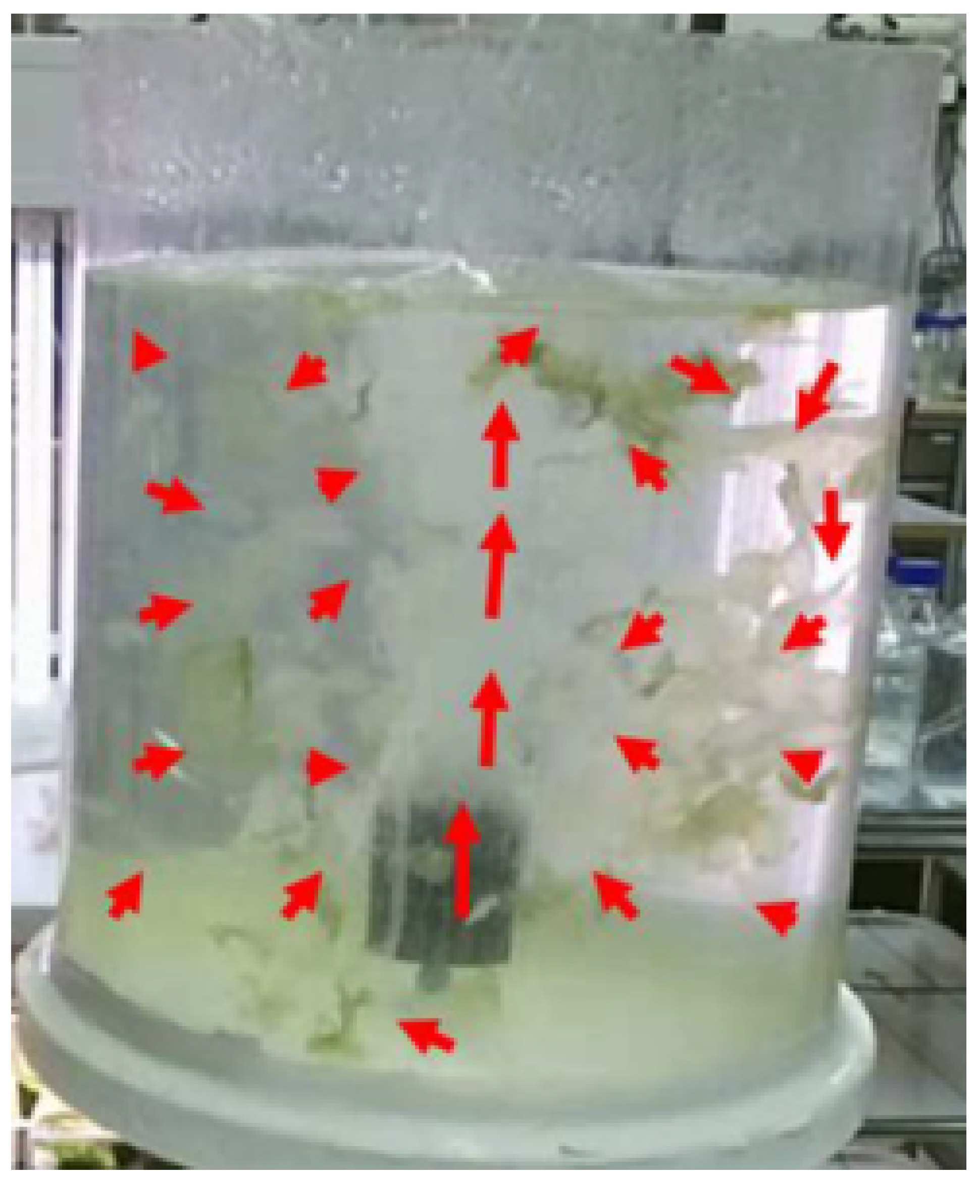
3.1. Experimental Setup

A suitable mixing system for macroalgae growing in aerated tanks was studied experimentally in [20] using three configurations (see Figure 1). In that study, Oca et al. developed three laboratory tanks for macroalgae culture that combined two geometrical configurations and two mixing systems. In this study, we took the vertical cylindrical (CV) setup with bottom aeration only, since it is the most used configuration for cultivating seaweed Ulva ohnoi. The tank depicted in Figure 2 was used for both the CFD numerical simulations and experimental measurements of the fluid flow; the latter serving the purpose of verifying the CFD results [45]. It is assumed that the flow pattern of the liquid phase, which induces the motion of the solid phase (modeled as a clump of particles via the DEM approach), could be improved (regularized) by inserting the cylindrical assembly (see Figure 2). Hence, the following hypothesis is proposed:

Hypothesis 1.

The inner cylindrical assembly (see Figure 2) makes a more regular flow pattern of the liquid phase. Consequently, the period of cyclic motion of the seaweed frond decreases when compared with the flow in the tank without the cylindrical assembly.

3.2. Seaweed Ulva ohnoi Cultivation Experiment

A cultivation experiment was performed using a cylindrical aerated tank for a summer school project, Computational and experimental assessment of the flow pattern within a macroalgae production system. The equipment consisted of an aerated tank with a diameter $D_C$ of 200 mm, and the water level height was equally set to 200 mm, which represents a volume of 6.3 L. The air volume rate (bottom aeration) was set to approximately 50 L/h. The seaweed Ulva ohnoi was provided by the Aquaculture Laboratories of the Universitat Politècnica de Catalunya in Castelldefels (UPC BarcelonaTech, Barcelona, Spain), where Ulva ohnoi was cultivated in cylindrical tanks illuminated from the water surface with irradiances ranging from 160 to 1000 micromol photons m⁻² s⁻¹. The seaweed stocking densities and the incident irradiance on the water surface were combined to obtain fronds with different chlorophyll contents. The results of the growth experiments were presented in the framework of summer schools in Nové Hrady, Czech Republic, established in 2002 by the University of South Bohemia, Institute of Physical Biology, and in 2012 by the Institute of Complex Systems (ICS).

Within the frame of the above-mentioned summer school project, a special purpose image processing method implemented in MATLAB R2020b (developed by Dr. Petr Císař, ICS, FFPW, University of South Bohemia, see [46] for more details), was used to visualize the flow pattern. The image processing results are shown in Figure 3, where the magnitude and direction of the red arrows determine the seaweed velocity. It is visible that a concentric loop was created from top to bottom, which in 3D could be visualized as a toroidal shape.

3.3. CFD Setup

In general, the problem of accurately simulating a multiphase flow involving fluid–structure interactions (FSIs) constitutes a significant challenge concerning mathematical modeling, numerical discretization, solution techniques, and implementation using software tools within modern computer architectures [47]. This is an even more challenging problem when the solid structure is highly flexible, as in the case of multiphase flow in aerated tanks with macroalgae. Nevertheless, currently, CFD packages such as ANSYS Fluent [25] or Star−CCM+ [26] possess a suitable Lagrangian–Eulerian method [32] describing the mutual interactions of a structure within the bulk liquid flow for different operating conditions, e.g., air flow rates. While some background about the multiphase flow and DEM approach was presented in Section 2, the basic settings for further CFD simulations coupled with DEM are described below.

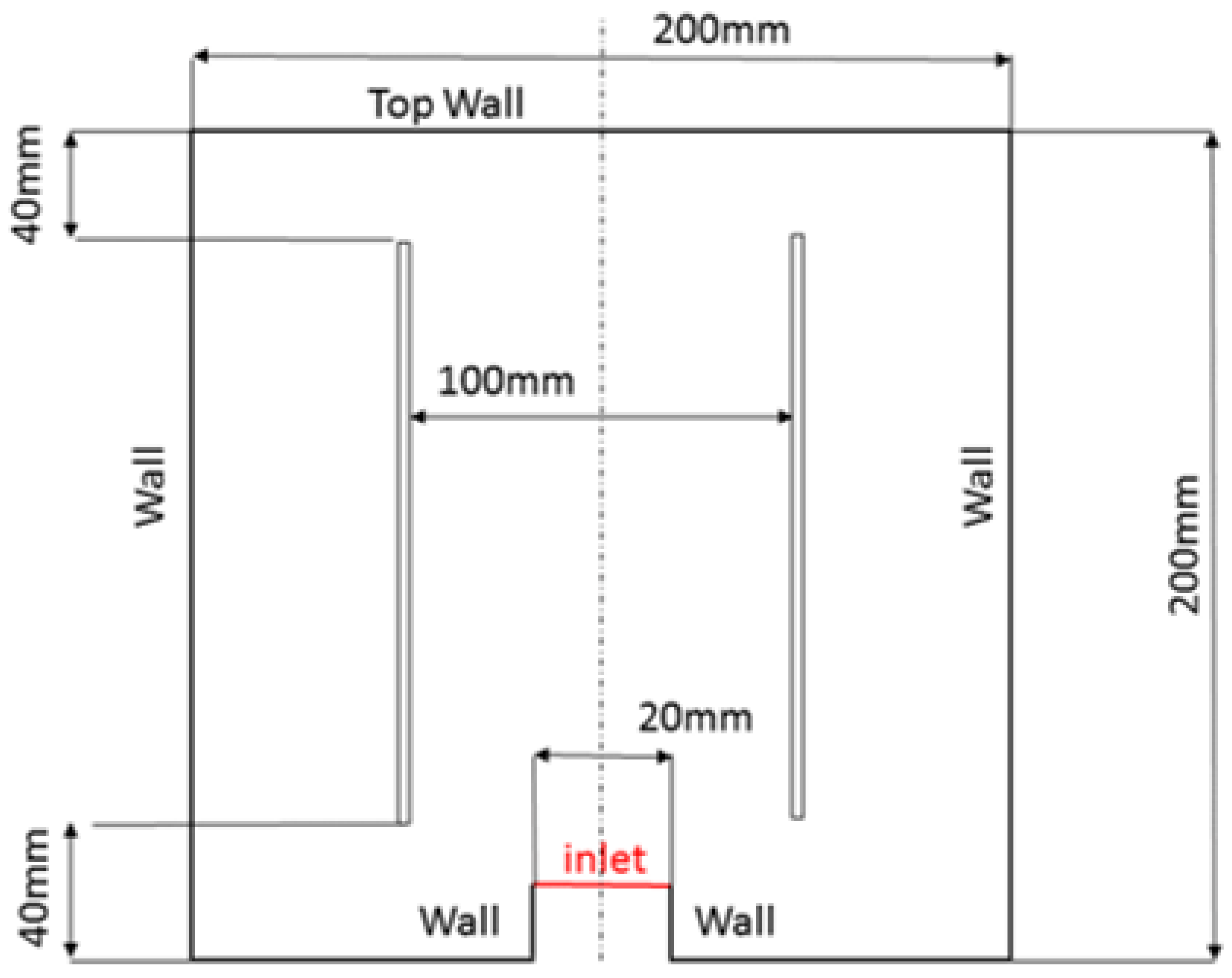
3.3.1. Geometry, Mesh Generation

According to our working hypothesis given in Section 3.1, using the inner cylindrical assembly (see Figure 2) promises a better flow pattern for macroalgae growth. Thus, two sets of geometry are used for both the 2D and 3D domains: one set with the inner cylindrical assembly and the other without. Considering the computational time needed for 3D simulations, the CFD model was treated as 2D, while the 3D domain and subsequent calculations were performed for the 2D results verification only. The 2D representation of the inner cylinder (axial cross-section of the 3D geometry) is viewed as two baffles in a squared vessel (see Figure 2). The thickness of the baffles corresponds to the width of one mesh cell.

3.3.2. Boundary Conditions for the 2D and 3D Models

To analyze the flow field in the geometrical domain for different operating conditions, the volume flow rate of air (aeration rate) was set up as a variable. However, in most simulations, the air volume flow rate was set to $\dot{V}=50\mathrm{L}/\mathrm{h}$. In the process of seeking the regression model for the relation between the time of one cycle of macroalgae motion and the specific aeration rate, the air volume flow rate covered the following values: $\{10;25;50;75;100\}$ L/h. Given that in Star−CCM+, the 2D model (with the DEM approach) assumes the third dimension (depth) to be 1 m, the air volume flow rate for the 2D domain needs to be recalculated appropriately to be consistent with the 3D geometry. To maintain the same ratio of the air volume flow rate and the tank volume for both 2D and 3D domains, the value for the 2D domain needs to be recalculated according to the following equation: ${\displaystyle \frac{{\dot{V}}_{2D}}{V_{2D}}}={\displaystyle \frac{{\dot{V}}_{3D}}{V_{3D}}}$, where $V_{2D}={D_C}^2·1$, and $V_{3D}={\displaystyle \frac{\pi {D_C}^3}{4}}$. The air volume flow rate for the 2D domain is then recalculated appropriately according to the following equation:

$${\dot{V}}_{2D}={\displaystyle \frac{4{\dot{V}}_{3D}}{\pi D_C}}.$$

(6)

3.3.3. CFD–DEM Coupling

The method that best suits particle tracking like macroalgae is the Lagrangian approach with the discrete element method (DEM). DEM particle clump model simulations can become very expensive to run when many particles are introduced into the domain, and also because each particle may need a very small time step to track properly. When considering the thickness of the macroalgae such as Ulva ohnoi, which can be less than 0.1 mm, the number of particles would be countless to cover some visible area. Thus, the computational time would dramatically rise. However, some methods can deliver results within a reasonable time. The flow field will be initialized with the steady-state two-phase flow, where the gas phase will be modeled using the Lagrangian multiphase model. Then, the transient physics with the DEM model and particle tracking will be applied. The flow field in the cylindrical tank will also be simulated using the inner cylinder assembly, which is expected to improve the flow field for macroalgae growing purposes.

The following assumptions and simplifications are further imposed:

• The macroalgae geometry is approximated with chains of spheres; the details are shown in Figure 4.

Figure 4. Illustrative picture of 2D simulation of the macroalgae motion. Macroalgae are modeled as particle clumps (see Detail) using the DEM approach (available in CFD code Star−CCM+). The scale of velocities for the solid and liquid phases are on each picture’s left and right-hand sides, respectively. The formation of rotating flow cells in the tank’s vertical section is observed (the particle track path is visualized with grey lines).

Figure 4. Illustrative picture of 2D simulation of the macroalgae motion. Macroalgae are modeled as particle clumps (see Detail) using the DEM approach (available in CFD code Star−CCM+). The scale of velocities for the solid and liquid phases are on each picture’s left and right-hand sides, respectively. The formation of rotating flow cells in the tank’s vertical section is observed (the particle track path is visualized with grey lines).

2.

The diameter of the spheres is set to 3 mm to maintain a low computational time.

3.

To prove the DEM concept, firstly, the 2D model was created and tested. Then, the 3D model was created and launched to verify the data from the 2D models.

4.

It is assumed that the particle (solid) movement will not change the flow pattern of the liquid phase, and the interaction between the gas and solid phases can be neglected (single-phase flow).

5.

The material properties for the CFD model have been set to ensure particle cohesion, flexibility, and a low computational time. The solid phase density is 1000 kg/m³, the elasticity modulus $E=$ 10 kPa, and Poisson’s ratio ${\mu }_P=0.1$.

6.

The densities of the liquid and gaseous phases, i.e., water and air, are set to 1000 kg/m³ and 1.18 kg/m³, respectively. The dynamic viscosity of water is set to 0.9 Pa·s.

7.

The flow field is steady and does not change over time.

3.3.4. CFD Solver Settings

A steady-state physics model was used to initialize the flow field. Then, the transient physics model was used for the DEM particle tracking. If parallel computation is used, enabling load balancing for both physics models is convenient. It is located in the Lagrangian multiphase solver, and it will reduce computational time. While using the transient physics, the time step was set to 0.01 s, and the segregated flow solver was set to be frozen. The other settings were left as the defaults. Physical time was chosen according to the flow field, which can capture several turns of the particles. It can vary from 15 to 80 s.

4. CFD Simulation Results and Discussion

This section compares and describes the velocity fields of the liquid phase for two alternative setups (with and without the inner cylinder). Then the particle tracks are presented and further processed.

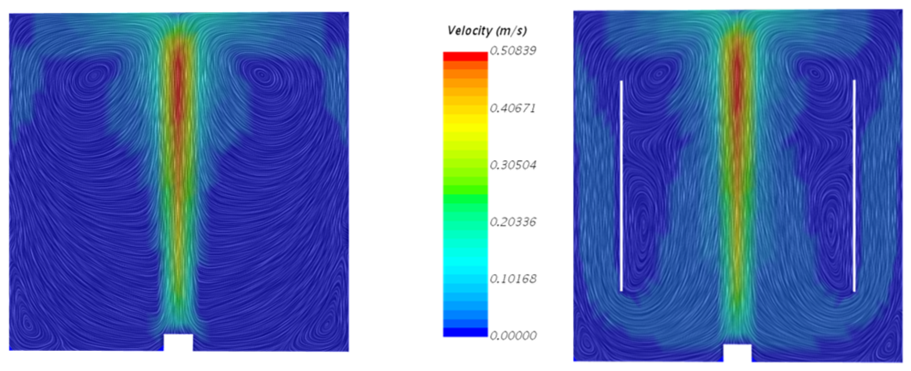
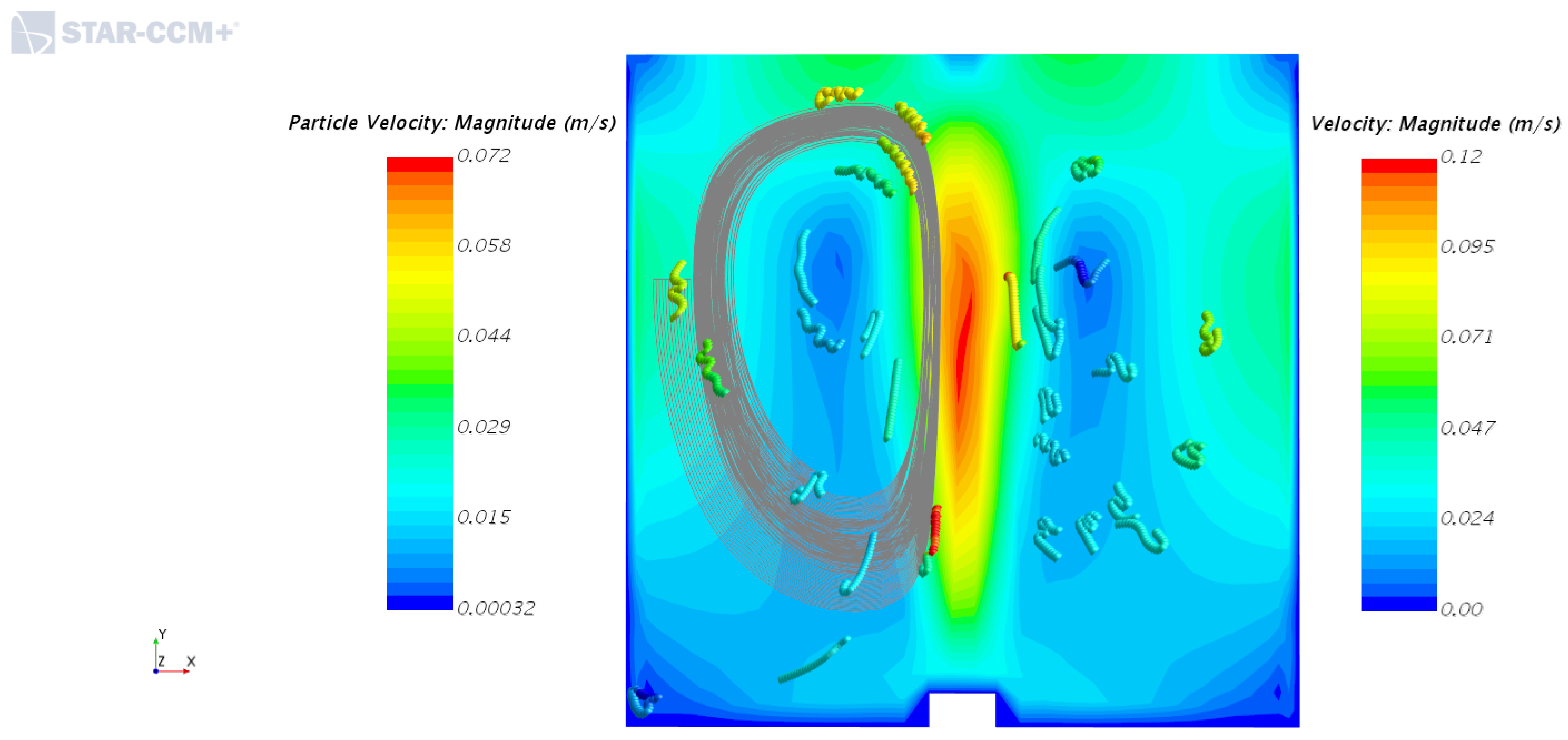
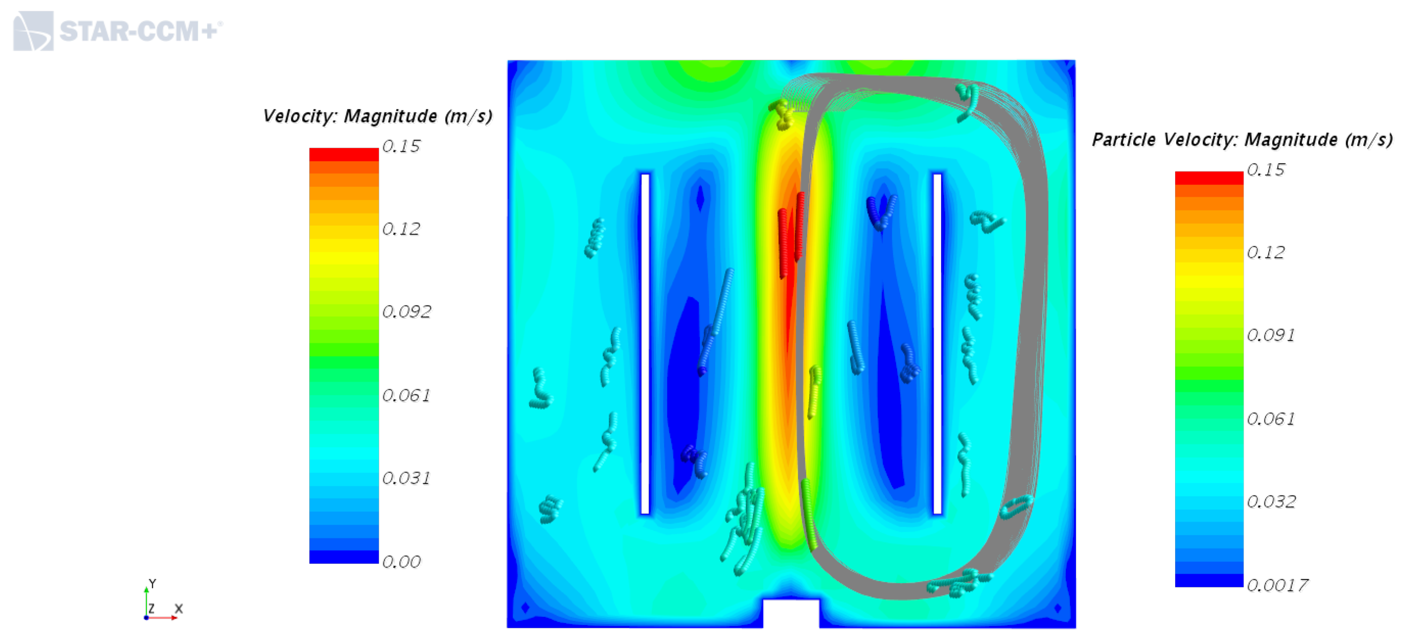
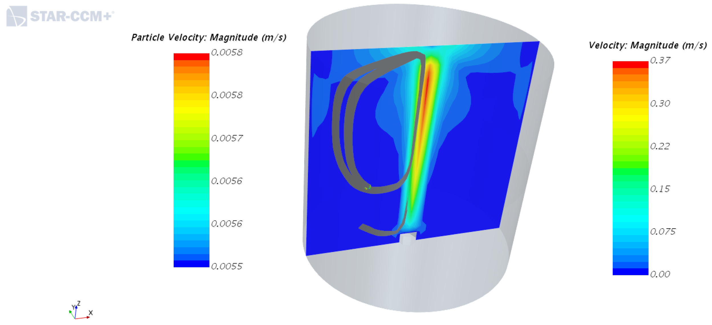
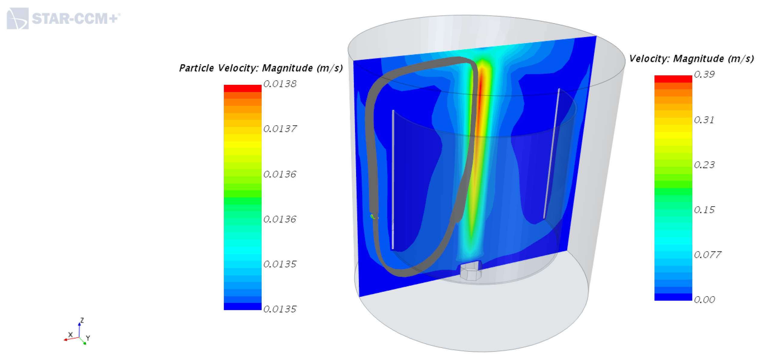
4.1. Velocity Fields of Liquid Phase with and without the Inner Cylinder Assembly

As an example of the influence of the effects of the inner cylindrical assembly on the tank hydrodynamics, the liquid velocity field for the aeration rate $\dot{V}=100\mathrm{L}/\mathrm{h}$ is depicted in the tank cross-section and presented in Figure 5. The results show that the inner cylindrical assembly significantly helps to distribute the velocity field to the bottom part of the domain and provides better conditions for recirculation than the domain without the inner cylinder. Although multiple concentric vortexes can be seen in Figure 5 (right), the majority of the fluid flows around the inner cylinder assembly, increasing the velocity in the tank’s bottom (not illuminated) part.

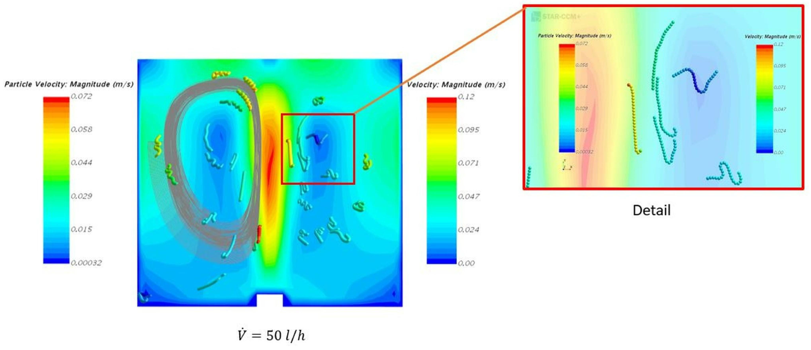
4.2. Solid Particle Tracking—Solid Phase Motion with and without the Inner Cylinder Assembly

To describe the macroalgae motion within the cylindrical, bottom aerated tank (with and without the inner cylinder assembly), we randomly injected (always for the 2D case) 31 particle clumps into the previously developed velocity field of the liquid phase. Particle tracking was applied on one particle clump, and its path can be seen in Figure 6 and Figure 7 for the domains without and with the inner cylinder, respectively. The figures show that using the inner cylindrical assembly provides a better distribution of particles inside the domain and more regular periodicity. This claim is also supported by visualization of the vertical position of the particles in time, shown in Figure 8 (in the next Section 4.3), i.e., more regular periodicity is observed with the usage of the inner cylinder.

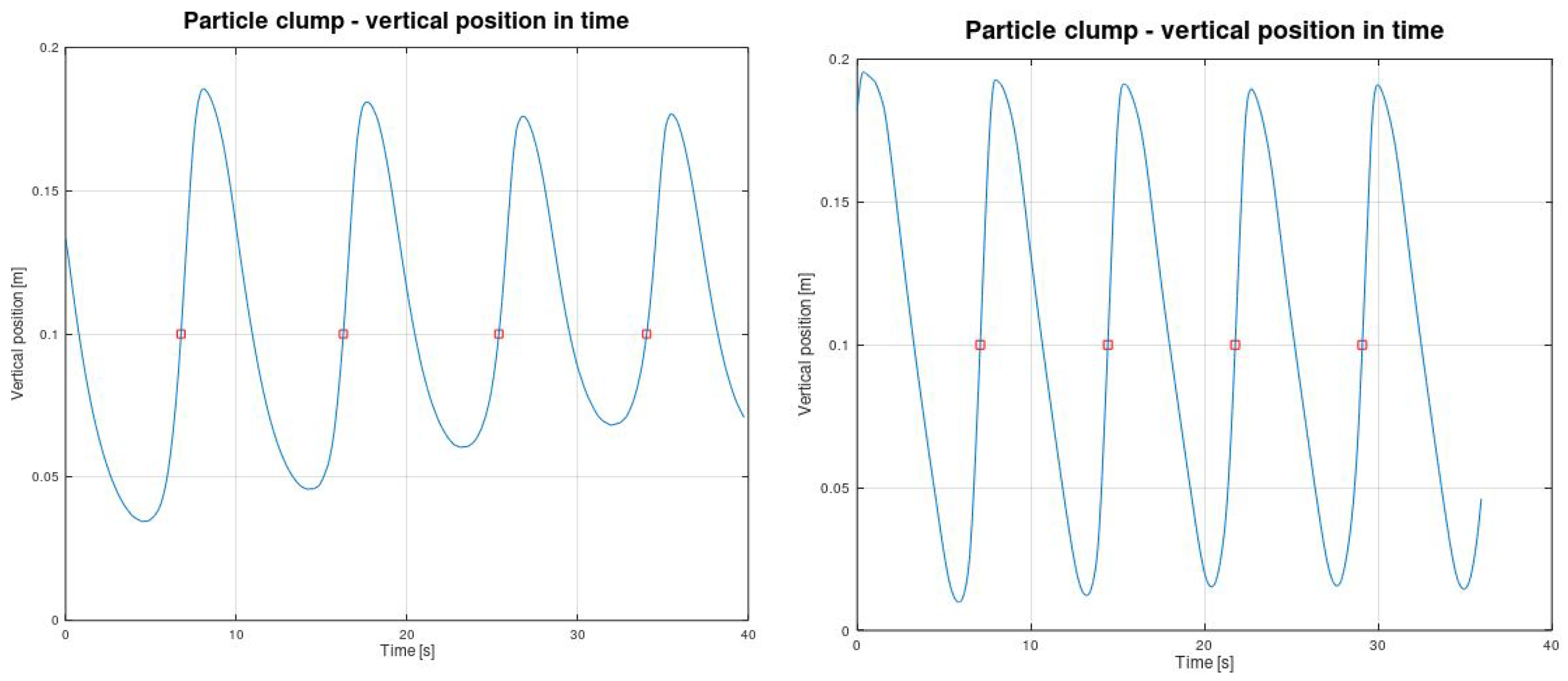
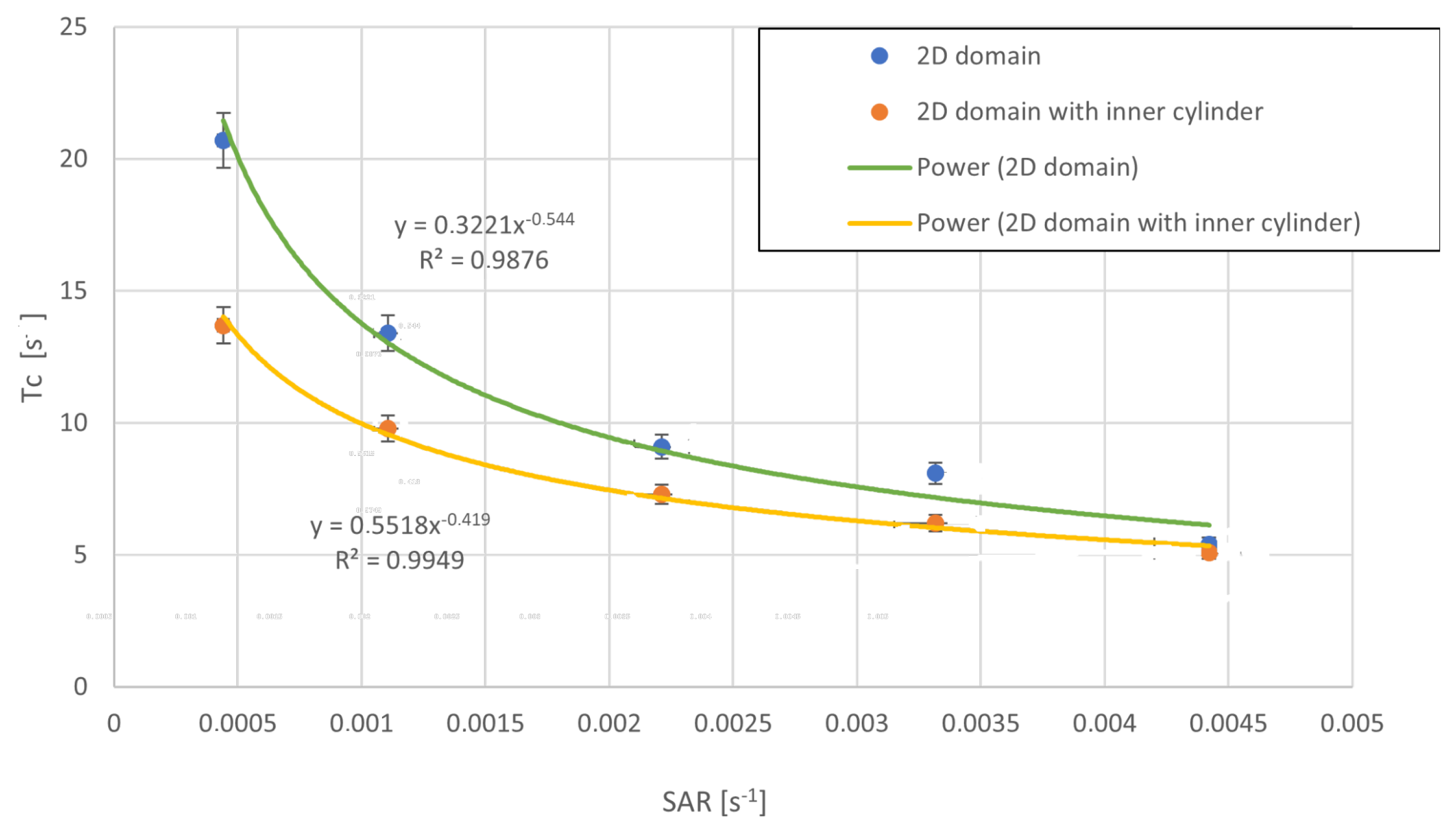
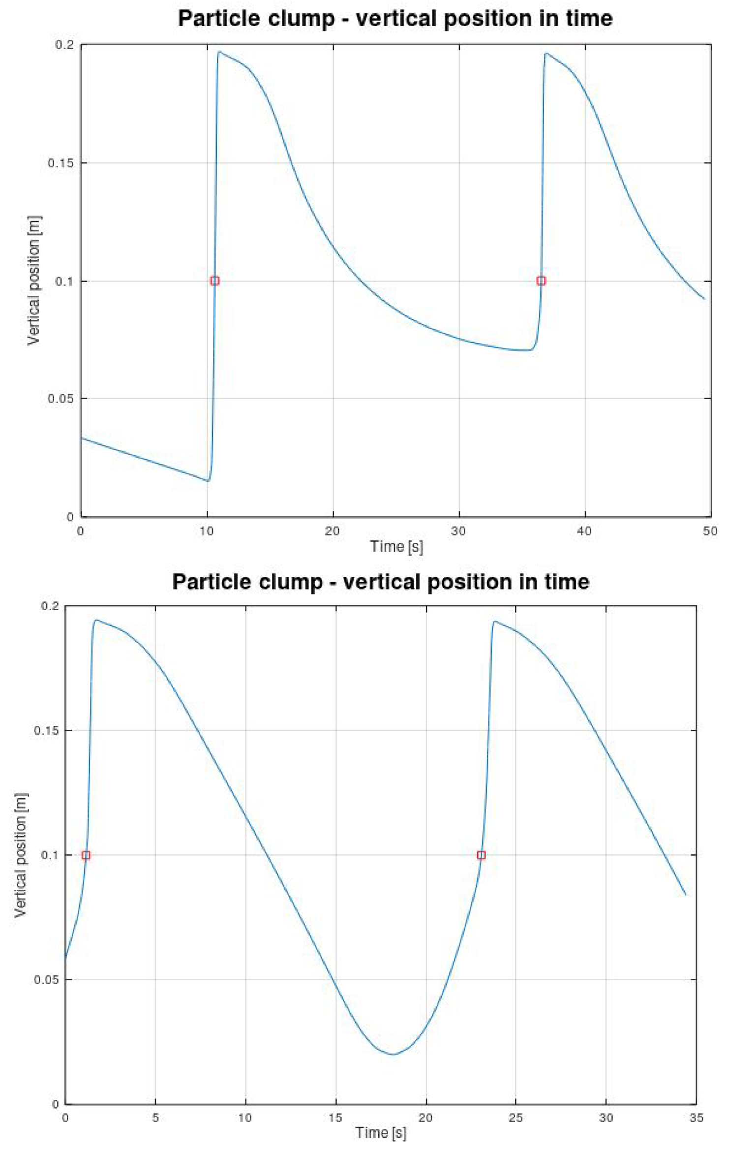
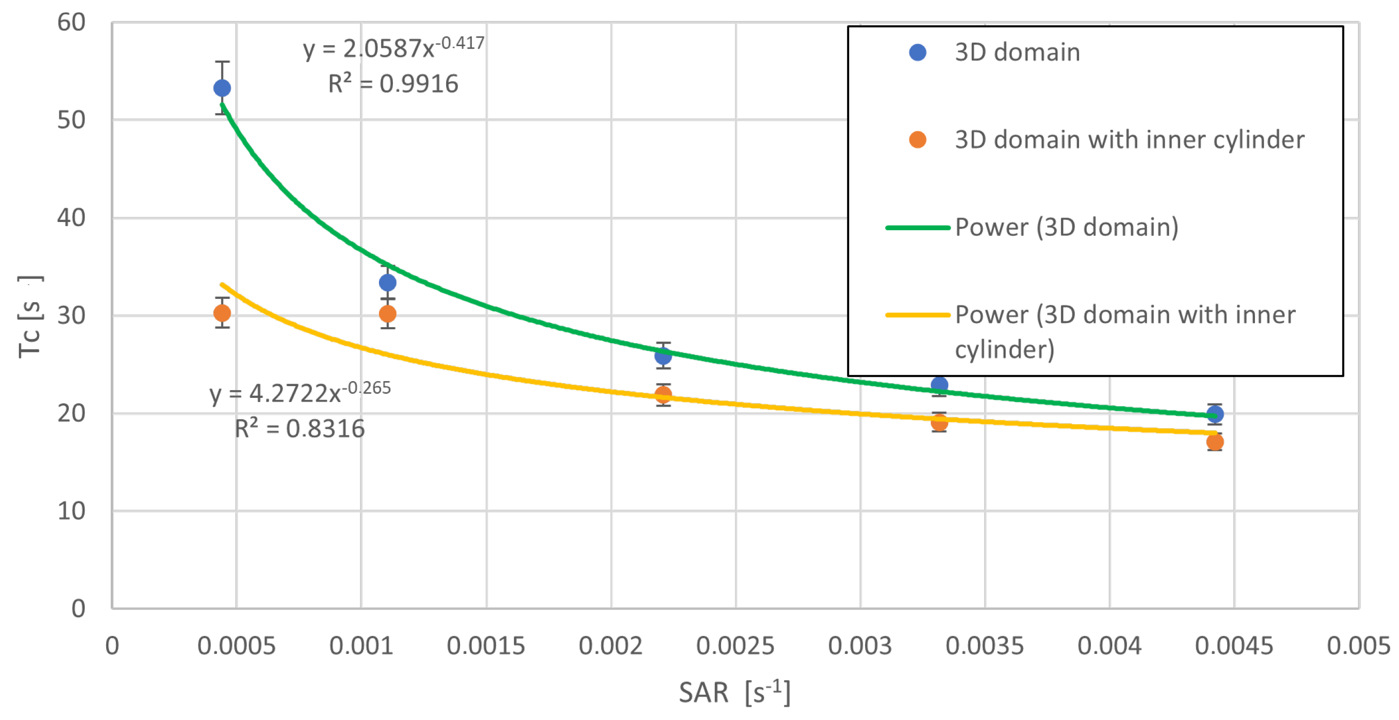
4.3. Post-Processing of Clump Trajectories

Based on the selected clump trajectories, the probabilistic description of the random variable describing the vertical position of a specific point in a particle clump (representing the center of mass of one single macroalgae) can be assessed; see Figure 8 (left) and (right) for the assembly without and with the inner cylinder (and the only one aeration rate 50 L/h), respectively. In this input–output relationship, the independent variable (or the input variable controlling the output variable $T_c$) is the aeration rate in a certain normalized form; see the next paragraph. Once the macroalgae motion is described, the so-called irradiance history is determined by a simple concatenation of the macroalgae trajectory and the irradiance field within the tank [42]. Consequently, the light regime (defined and described in Section 2.4) can be extracted from the irradiance history as an input to a model describing the photosynthetic growth.

First, the so-called specific aeration rate (SAR, units $\left[{\mathrm{s}}^{-1}\right]$) is defined as follows:

$$SAR=\dot{V}/V,$$

(7)

where $\dot{V}$ is the air volume flow rate, as described in Section 3.3, and V is the tank volume. To have a regression model for the relation between the period of the cycle $T_c$ and the specific aeration rate, new data from CFD simulations were obtained based on the variations in the air volume flow rates. The data were post-processed using Matlab/Octave code, which plots the particle’s vertical position in time. Two examples for cases without and with inner assembly are shown in Figure 8 (left) and (right), respectively. Next, the average value of the time period for the particle to complete one cycle was determined. This value can be understood as the mean value of the random variable $T_c$, i.e., the mean period of an intermittent macroalgae illumination process.

Finally, two simple mathematical relations were identified:

$$T_c=0.3221{\left({\displaystyle \frac{\dot{V}}{V}}\right)}^{-0.54},$$

(8)

for the 2D system without the inner cylinder assembly, and

$$T_c=0.5518{\left({\displaystyle \frac{\dot{V}}{V}}\right)}^{-0.42}.$$

(9)

for the 2D system with the inner cylinder assembly, see Figure 9 for the graphical representation.

In the 3D case, only one particle clump, see Figure 10, was randomly injected into the velocity field. Afterward, the visualization of CFD data as particle paths can be observed in Figure 11 for the domain without an inner cylinder and in Figure 12 for the domain with an inner cylinder, respectively. Again, similar to the 2D domain, both figures show that using the inner cylinder assembly enhances the distribution of the particle clumps over the domain.

Similarly to the 2D case, the vertical position of the particles in the time plots for the cases without and with the inner assembly are shown in Figure 13 (top) and (bottom), respectively, and the power functions (10) and (11) were identified for the 3D domain:

$$T_c=2.06{\left({\displaystyle \frac{\dot{V}}{V}}\right)}^{-0.42},$$

(10)

for the 3D system without the inner cylinder assembly and

$$T_c=4.27{\left({\displaystyle \frac{\dot{V}}{V}}\right)}^{-0.265}.$$

(11)

for the 3D system with the inner cylinder assembly. Again, it can be well observed in the graphical picture given in Figure 14 that the cycle period $T_c$ is lower for the case with the inner cylinder inserted, although as the aeration rate increases, the difference between both cases decreases.

As the final comment, we emphasize that the issue of verification of CFD numerical simulations and the validation of the whole modeling approach is out of the scope of this work, which is conceptualized as a proof-of-concept study. A guide for estimating uncertainty due to discretization in CFD applications is available in ref. [45].

5. Conclusions

The movement of seaweed in aerated tanks is a crucial factor for the radiation interception by seaweed fronds, which will have a noteworthy influence on the yield. Therefore, we aimed to use a commercial CFD code to describe and test one promising approach to modeling aerated (or bubbled) systems for macroalgae cultivation, e.g., integrated into IMTA systems. It was found that the approach that was best suited for modeling the macroalgae movement within those systems was to use the discrete element method (DEM) with a particle clumps model. This model is included in the Star−CCM+ code used for the analysis presented here.

Thus, we tested the CFD-DEM method to model macroalgae cultivation in aerated tanks. Considering the geometrical dimension, two branches of models of aerated systems were created, one 2D and one 3D. Both were supposed to represent the aerated cylindrical tank, but in the case of the 2D model, due to the incompatibility of an axisymmetric model with the DEM approach in Star−CCM+ code, the 2D model represented a rectangular vessel rather than a vertical cylindrical tank.

As a practical goal, this proof-of-concept study aimed to analyze the hypothesis regarding the beneficial role of using an inner assembly inside the aerated tank. For this purpose, the 2D model was used because of its good precision and low computational cost. Afterward, the results of the 2D CFD simulations showed that the inner assembly provided better distribution of the velocity field inside the tank, and it could reduce the time the macroalgae needed for one cycle of their periodic motion. Furthermore, a simple mathematical relation was derived, describing the correlation between the macroalgae’s cycle period (in the vertical cross-section, the macroalgae move between the illuminated surface and the dark bottom) and the specific aeration rate for either the 2D and 3D domain (see Equations (8)–(11)). These correlations are needed to assess production systems’ biological performance and eventually to set up the optimal conditions for macroalgae cultivation.

Although the created models represent a humble beginning, it has been shown that it is possible to model the aerated systems with macroalgae. Nevertheless, as far as we know, this work represents one of the first research studies dedicated to applying coupled CFD and DEM approaches in aerated tanks with seaweed, such as the ones used in IMTA-RAS systems. Still, many assumptions and simplifications were made (see Section 3.3), so the accuracy level is questionable. Indeed, experimental measurement of material properties such as the elasticity modulus E and Poisson’s ratio ${\mu }_P$ for the specimens extracted from the specific macroalgae fronds and the subsequent macroalgae motion within the aerated tanks used to calibrate the numerical models must be performed to validate the CFD results fully. This is planned for the near future as an independent study. Nevertheless, the first step was made using the image processing software developed in the Institute of Complex Systems of the University of South Bohemia in České Budějovice, Czech Republic.

References

1. Neori, A.; Chopin, T.; Troell, M.; Buschmann, A.H.; Kraemer, G.P.; Halling, C.; Shpigel, M.; Yarish, C. Integrated aquaculture: Rationale, evolution and state of the art emphasizing seaweed biofiltration in modern mariculture. Aquaculture 2004, 231, 361–391. [Google Scholar] [CrossRef]
2. Neori, A. Essential role of seaweed cultivation in integrated multi-trophic aquaculture farms for global expansion of mariculture: An analysis. J. Appl. Phycol. 2008, 20, 567–570. [Google Scholar] [CrossRef]
3. Neori, A.; Shpigel, M.; Guttman, L.; Israel, A. Development of polyculture and integrated multi-trophic aquaculture (IMTA) in Israel: A review. Isr. J. Aquac. 2017, 69, 1–19. [Google Scholar] [CrossRef]
4. Wu, X.; Merchuk, J.C. Simulation of algae growth in a bench-scale bubble column reactor. Biotechnol. Bioeng. 2002, 80, 156–168. [Google Scholar] [CrossRef] [PubMed]
5. Petera, K.; Papáček, Š.; González, C.I.; Fernández-Sevilla, J.M.; Acién Fernández, F.G. Advanced Computational Fluid Dynamics Study of the Dissolved Oxygen Concentration within a Thin-Layer Cascade Reactor for Microalgae Cultivation. Energies 2021, 14, 7284. [Google Scholar] [CrossRef]
6. Inostroza, C.; Papáček, S.; Fernández-Sevilla, J.; Acién, F.G. Optimization of thin-layer photobioreactors for the production of microalgae by integrating fluid-dynamic and photosynthesis rate aspects. J. Appl. Phycol. 2023, 35, 2111–2123. [Google Scholar] [CrossRef]
7. Martínez, E.C.; Kim, J.W.; Barz, T.; Cruz Bournazou, M.N. Probabilistic Modeling for Optimization of Bioreactors using Reinforcement Learning with Active Inference. In ESCAPE-31, Proceedings of the 31st European Symposium on Computer Aided Process Engineering, Istanbul, Turkey, 6–9 June 2021; Türkay, M., Gani, R., Eds.; Computer Aided Chemical Engineering; Elsevier: Amsterdam, The Netherlands, 2021; Volume 50, pp. 419–424. [Google Scholar] [CrossRef]
8. Martins, C.; Eding, E.; Verdegem, M.; Heinsbroek, L.; Schneider, O.; Blancheton, J.; d’Orbcastel, E.R.; Verreth, J. New developments in recirculating aquaculture systems in Europe: A perspective on environmental sustainability. Aquac. Eng. 2010, 43, 83–93. [Google Scholar] [CrossRef]
9. Edwards, P. Aquaculture environment interactions: Past, present and likely future trends. Aquaculture 2015, 447, 2–14. [Google Scholar] [CrossRef]
10. Hadley, S.; Wild-Allen, K.; Johnson, C.; Macleod, C. Modeling macroalgae growth and nutrient dynamics for integrated multi-trophic aquaculture. J. Appl. Phycol. 2015, 27, 901–916. [Google Scholar] [CrossRef]
11. Knowler, D.; Chopin, T.; Martínez-Espiñeira, R.; Neori, A.; Nobre, A.; Noce, A.; Reid, G. The economics of Integrated Multi-Trophic Aquaculture: Where are we now and where do we need to go? Rev. Aquac. 2020, 12, 1579–1594. [Google Scholar] [CrossRef]
12. Oca, J.; Cremades, J.; Jiménez, P.; Pintado, J.; Masaló, I. Culture of the seaweed Ulva ohnoi integrated in a Solea senegalensis recirculating system: Influence of light and biomass stocking density on macroalgae productivity. J. Appl. Phycol. 2019, 31, 2461–2467. [Google Scholar] [CrossRef]
13. Msuya, F.; Kyewalyanga, M.; Salum, D. The performance of the seaweed Ulva reticulata as a biofilter in a low-tech, low-cost, gravity generated water flow regime in Zanzibar, Tanzania. Aquaculture 2006, 254, 284–292. [Google Scholar] [CrossRef]
14. Kok, B. Experiments on photosynthesis by Chlorella in flashing light. In Algal Culture from Laboratory to Pilot Plant; Burlew, J., Ed.; Carnegie Institute: Washington, DC, USA, 1953; Volume 600, pp. 63–75. [Google Scholar]
15. Terry, K.L. Photosynthesis in modulated light: Quantitative dependence of photosynthetic enhancement on flashing rate. Biotechnol. Bioeng. 1986, 28, 988–995. [Google Scholar] [CrossRef]
16. Grobbelaar, J.; Nedbal, L.; Tichý, V. Influence of high frequency light/dark fluctuations on photosynthetic characteristics of microalgae photoacclimated to different light intensities and implications for mass algal cultivation. J. Appl. Phycol. 1996, 8, 335–343. [Google Scholar] [CrossRef]
17. Nedbal, L.; Tichý, V.; Xiong, F.; Grobbelaar, J. Microscopic green algae and cyanobacteria in high-frequency intermittent light. J. Appl. Phycol. 1996, 8, 325–333. [Google Scholar] [CrossRef]
18. Ginovart, M.; Pintado, J.; Del Olmo, G.; Cremades, J.; Jiménez, P.; Masaló, I. Light distribution in tanks with the green seaweed Ulva ohnoi: Effect of stocking density, incident irradiance and chlorophyll content. J. Appl. Phycol. 2023, 35, 1995–2006. [Google Scholar] [CrossRef]
19. Luo, H.P.; Kemoun, A.; Al-Dahhan, M.H.; Sevilla, J.; Sánchez, J.; Camacho, F.; Grima, E. Analysis of photobioreactors for culturing high-value microalgae and cyanobacteria via an advanced diagnostic technique: CARPT. Chem. Eng. Sci. 2003, 58, 2519–2527. [Google Scholar] [CrossRef]
20. Oca, J.; Machado, S.; Jimenez de Ridder, P.; Cremades, J.; Pintado, J.; Masaló, I. Comparison of two water agitation methods in seaweed culture tanks: Influence of the rotating velocity in the seaweed growth and energy requirement. In Proceedings of the EAS2016—Food for Thought, Edinburgh, UK, 20–23 September 2016; pp. 716–717. [Google Scholar]
21. Traugott, H.; Zollmann, M.; Cohen, H.; Chemodanov, A.; Liberzon, A.; Golberg, A. Aeration and nitrogen modulated growth rate and chemical composition of green macroalgae Ulva sp. cultured in a photobioreactor. Algal Res. 2020, 47, 101808. [Google Scholar] [CrossRef]
22. Bitog, J.; Lee, I.B.; Lee, C.G.; Kim, K.S.; Hwang, H.S.; Hong, S.W.; Seo, I.H.; Kwon, K.S.; Mostafa, E. Application of Computational Fluid Dynamics for Modeling and Designing Photo-Bioreactors: For Microalgae Production: A Review. Comput. Electron. Agric. 2011, 76, 131–147. [Google Scholar] [CrossRef]
23. Park, S.; Li, Y. Integration of biological kinetics and computational fluid dynamics to model the growth of Nannochloropsis salina in an open channel raceway. Biotechnol. Bioeng. 2015, 112, 923–933. [Google Scholar] [CrossRef]
24. Ranganathan, P.; Pandey, A.K.; Sirohi, R.; Tuan Hoang, A.; Kim, S.H. Recent advances in computational fluid dynamics (CFD) modelling of photobioreactors: Design and applications. Bioresour. Technol. 2022, 350, 126920. [Google Scholar] [CrossRef] [PubMed]
25. ANSYS Fluent. ANSYS Fluent Theory Guide; ANSYS, Inc.: Canonsburg, PA, USA, 2017. [Google Scholar]
26. Siemens Digital Industries Software. Simcenter STAR-CCM+ Product Documentation. 2018. Available online: https://www.plm.automation.siemens.com/global/en/products/simcenter/STAR-CCM.html (accessed on 16 May 2024).
27. Hurd, C.L. Water Motion, Marine Macroalgal Physiology, and Production. J. Phycol. 2000, 36, 453–472. [Google Scholar] [CrossRef] [PubMed]
28. Koehl, M.A.R. Seaweeds in Moving Water: Form and Function. In On the Economy of Plant Form and Function; Givnish, T.J., Ed.; Cambridge University Press: Cambridge, UK, 1986; pp. 603–634. [Google Scholar]
29. Spatz, H.C.; Köhler, L.; Niklas, K.J. Mechanical behaviour of plant tissues: Composite materials or structures? J. Exp. Biol. 1999, 202, 3269–3272. [Google Scholar] [CrossRef] [PubMed]
30. Burnett, N.P.; Koehl, M.A.R. Mechanical properties of the wave-swept kelp Egregia menziesii change with season, growth rate and herbivore wounds. J. Exp. Biol. 2019, 222, jeb190595. [Google Scholar] [CrossRef] [PubMed]
31. Bolton, J.J.; Cyrus, M.D.; Brand, M.J.; Joubert, M.; Macey, B.M. Why grow Ulva? Its potential role in the future of aquaculture. Perspect. Phycol. 2016, 3, 113–120. [Google Scholar] [CrossRef]
32. Subramaniam, S. Lagrangian–Eulerian methods for multiphase flows. Prog. Energy Combust. Sci. 2013, 39, 215–245. [Google Scholar] [CrossRef]
33. Farivar, F.; Zhang, H.; Tian, Z.F.; Gupte, A. CFD-DEM simulation of fluidization of multisphere- modelled cylindrical particles. Powder Technol. 2020, 360, 1017–1027. [Google Scholar] [CrossRef]
34. Zhu, H.; Zhou, Z.; Yang, R.; Yu, A. Discrete particle simulation of particulate systems: A review of major applications and findings. Chem. Eng. Sci. 2008, 63, 5728–5770. [Google Scholar] [CrossRef]
35. Johnson, K. Contact Mechanics; Cambridge University Press: Cambridge, UK, 1987. [Google Scholar]
36. Rayleigh, L. On Waves Propagated along the Plane Surface of an Elastic Solid. Proc. Lond. Math. Soc. 1885, s1–17, 4–11. [Google Scholar] [CrossRef]
37. Timoshenko, S.; Timoshenko, S.; Goodier, J. Theory of Elasticity; Timoshenko, S., Goodier, J.N., Eds.; McGraw-Hill Book Company: New York, NY, USA, 1951. [Google Scholar]
38. Merchuk, J.C.; Garcia-Camacho, F.; Molina-Grima, E. Photobioreactor Design and Fluid Dynamics. Chem. Biochem. Eng. Q. 2007, 21, 345–355. [Google Scholar]
39. Papáček, Š.; Štumbauer, V.; Štys, D.; Petera, K.; Matonoha, C. Growth impact of hydrodynamic dispersion in a Couette–Taylor bioreactor. Math. Comput. Model. 2011, 54, 1791–1795. [Google Scholar] [CrossRef]
40. Gao, X.; Kong, B.; Dennis Vigil, R. Comprehensive computational model for combining fluid hydrodynamics, light transport and biomass growth in a Taylor vortex algal photobioreactor: Eulerian approach. Algal Res. 2017, 24, 1–8. [Google Scholar] [CrossRef]
41. Masojídek, J.; Koblížek, M.; Torzillo, G. Photosynthesis in Microalgae. In Handbook of Microalgal Culture; John Wiley & Sons, Ltd.: Hoboken, NJ, USA, 2003; Chapter 2; pp. 20–39. [Google Scholar] [CrossRef]
42. Papáček, Š.; Jablonsky, J.; Petera, K. Advanced integration of fluid dynamics and photosynthetic reaction kinetics for microalgae culture systems. BMC Syst. Biol. 2018, 12, 93. [Google Scholar] [CrossRef]
43. Molina, E.; Acién Fernández, F.G.; García Camacho, F.; Camacho Rubio, F.; Chisti, Y. Scale-up of Tubular Photobioreactors. J. Appl. Phycol. 2000, 12, 355–368. [Google Scholar] [CrossRef]
44. Burlew, J.S. Algal Culture from Laboratory to Pilot Plant; Carnegie Institution of Washington: Washington, DC, USA, 1953. [Google Scholar]
45. Celik, I.; Ghia, U.; Roache, P.; Freitas, C.; Coleman, H.; Raad, P. Procedure for Estimation and Reporting of Uncertainty Due to Discretization in CFD Applications. J. Fluids Eng. 2008, 130, 078001. [Google Scholar] [CrossRef]
46. Bekkozhayeva, D.; Cisar, P. Image-Based Automatic Individual Identification of Fish without Obvious Patterns on the Body (Scale Pattern). Appl. Sci. 2022, 12, 5401. [Google Scholar] [CrossRef]
47. Burnett, B. Coupled Fluid-Structure Interaction Modeling of a Parafoil. Master Thesis, Embryo-Riddle Aeronautical University, Daytona Beach, FL, USA, 2016. [Google Scholar]
Figure 1. Three laboratory experimental systems: vertical cylindrical (CV) tank; semi-spherical tank, bottom aerated (SH2); and semi-spherical tank with water jet system (SH1) [20].
Energies 17 03555 g001
Figure 2. Scheme of the cylindrical tank geometry depicted as the axial cross-section. The removable inner cylindrical assembly with a 100 mm diameter has an open top and bottom part and is elevated, allowing the flow of all three phases, i.e., water, gas bubbles, and macroalgae.
Energies 17 03555 g002
Figure 3. Experimental laboratory tank with bottom aeration for Ulva ohnoi cultivation. The image processing software (developed by the University of South Bohemia in České Budějovice, FFPW, Institute of Complex Systems in Nové Hrady, Czech Republic) colocates the arrows that determine the velocity of the macroalgae fronds.
Energies 17 03555 g003
Figure 5. Two typical examples of velocity fields of the liquid phase without (on the left) and with (on the right) the inner cylinder assembly extracted from CFD simulations. Air volume flow rate: 100 L/min.
Energies 17 03555 g005
Figure 6. Multiphase flow fields without the inner cylinder assembly extracted from 2D CFD simulations. Air volume flow rate: 50 L/min. The scale of velocities for the solid and liquid phases are on each picture’s left and right-hand sides. The particle track path is visualized with grey lines.
Energies 17 03555 g006
Figure 7. Multiphase flow fields with the inner cylinder assembly extracted from 2D CFD simulations. Air volume flow rate: 50 L/min. The scales of velocities for the solid and liquid phases are on each picture’s right and left-hand sides. The particle track path is visualized with grey lines.
Energies 17 03555 g007
Figure 8. Time course of the vertical position of the particle clump (seaweed frond) for the aeration rate of 50 L/h. (left) 2D domain without the inner cylinder. (right) 2D domain with the inner cylinder.
Energies 17 03555 g008
Figure 9. The relation between the period of the cycle T c and the specific aeration rate based on 2D simulations in CFD code Star−CCM+.
Energies 17 03555 g009
Figure 10. Detailed view fn a particle clump in the 3D domain. The plasticity of the particle clump can be observed, as it is shaped by the surrounding flow of liquid.
Energies 17 03555 g010
Figure 11. Multiphase 3D flow fields with an injected particle clump and without the inner cylinder assembly. The particle track path is visualized with grey lines.
Energies 17 03555 g011
Figure 12. Three-dimensional domain with inner cylindrical assembly and injected particle clump.
Energies 17 03555 g012
Figure 13. Time course of the vertical position of the particle clump for the 3D domain without the inner cylinder (top) and for the 3D domain with the inner cylinder (bottom).
Energies 17 03555 g013
Figure 14. The relation between the period of the cycle T c and the specific aeration rate based on 3D simulations in CFD code Star−CCM+.
Energies 17 03555 g014
Disclaimer/Publisher’s Note: The statements, opinions and data contained in all publications are solely those of the individual author(s) and contributor(s) and not of MDPI and/or the editor(s). MDPI and/or the editor(s) disclaim responsibility for any injury to people or property resulting from any ideas, methods, instructions or products referred to in the content.