Article

A Gap Nonlinearity Compensation Strategy for Non-Direct-Drive Servo Systems

by
Bo Wang
1,2,
Runze Ji
2,
Chengpeng Zhou
2,
Rana M. Sohel
2,
Kai Liu
2,*,
Wei Hua
2 and
Hairong Ye
2
1
Xi’an Modern Control Technology Institute, Xi’an 710065, China
2
School of Electrical Engineering, Southeast University, Nanjing 210096, China
*
Author to whom correspondence should be addressed.
Energies 2024, 17(14), 3582; https://doi.org/10.3390/en17143582
Submission received: 13 June 2024 / Revised: 14 July 2024 / Accepted: 17 July 2024 / Published: 21 July 2024
(This article belongs to the Section F3: Power Electronics)

Abstract

:
In this paper, a gap nonlinear compensation strategy is proposed for the full closed-loop control structure of non-direct-drive servo motor systems. Firstly, an improved deadband model containing the initial value of the gap is proposed, and two gap amplitude identification methods, namely, incremental torque and velocity difference integral, are compared. Then, for the full closed-loop structure, based on the describing function and the stability theory of the nonlinear system, the limit-loop oscillating frequency and the influencing factors are predicted, which are related to the system control stiffness and independent of the gap amplitude; finally, the state-feedback control is proposed, and the feedback coefficients are designed by using the pole configuration, making the system a pseudo-linear system. Simulation and experimental verification show that the method can suppress the limit loop oscillation, attenuate the system shock, and have a certain robustness.

1. Introduction

In servo non-direct drive systems, the existence of backlash is unavoidable. On the one hand, sufficient space must be reserved to fill with lubricant, etc., and on the other hand, it is also necessary to avoid the expansion and jamming of gears caused by thermal deformation. The existence of backlash introduces problems such as unknown initial position and space range during commutation, leading to poor positioning accuracy, and its nonlinear characteristics will also cause mechanical resonance, which can seriously endanger the system and personal safety. For this reason, it is necessary to use gap elimination methods for gap compensation. Gap elimination or compensation methods can be divided into two categories: mechanical gap elimination and control-strategy gap elimination. However, the whole process of mechanical backlash design is cumbersome, and additional equipment is costly and needs to be redesigned for different equipment and applications. Compensating for gap nonlinearity at the level of the control algorithm reduces mechanical dependence, simplifies the servo system structure, and improves operational reliability to some extent. Compensation algorithms are divided into two categories according to whether or not the gap magnitude needs to be known: compensation based on the gap model and compensation not based on the gap model.
Summarizing the research results of current scholars, feasible gap mathematical models include the hysteresis model [1], the dead-zone model [2], the approximate dead-zone [3] model, and the impulse model [4]. To establish the above models, the gap magnitude must be identified. When position sensors are installed on both the drive side and the load side, only the difference between the two needs to be compared (the transmission ratio needs to be considered) to derive the clearance value. The literature [5] uses two position sensors, with the gap value as one of the state quantities in the switching free state space, and the gap magnitude is estimated using the difference between the measured output and the Kalman observed output. Due to the limitations of installation conditions or to the inconsistent accuracy of sensors, completing the gap identification based on the drive motor-side position sensor only has become a hot spot of current research. The literature [6] summarizes four different identification methods based on the gap deadband model, including given smaller torque pulse, incremental torque pulse, quasi-static, and velocity difference integrals, and the experimental results prove the superiority of the velocity difference integral-based method, which is also adopted in this paper.
The idea of model-based compensation is to introduce the inverse of the model into the control signal and add the tracking error to the original expected value so that the controlled system is transformed into a pseudo-linear system [7], and this kind of method is also called inverse model compensation. To address the shortcomings of the classical non-frivolous model mentioned above, [8] the concept of ‘softness’ has been proposed to overcome the non-frivolous ‘hard’ nature of the traditional gap model so that the system can be a smooth transition between the gap mode and the mesh mode. However, the literature does not extend the ‘softness’ concept to the case where the gap is unknown, and further research on dynamic softening is needed.
In recent years, modern algorithms such as backstepping, adaptive, neural network, self-resistant, and robust control have been widely used in gap compensation [9]. The literature [10] discusses the fuzzy tracking control problem when the switching system is subject to an unknown input gap, non-constant control gain, and asymmetric full-state constraints, and in order to deal with the unknown input gap nonlinearity with unknown non-constant control gain function, a new parametric smoothing gap inverse based on the fuzzy logic system is proposed, but the design of this method is complicated, and the paper only provides simulation verification.
In addition to focusing on the gap, some experts and scholars focus on the direct elimination or suppression of responses such as mechanical resonance induced by the gap and design the system-transfer function by configuring the zero-pole and other ways to change the resonance frequency point [3], to improve the dynamic and steady-state performance of the system. The literature [11] discusses the design of a robust shaft torque compensator to approximate a rigid system and attenuate mechanical resonance by limiting the amplitude of the shaft torque, but the scholar had a problem with the substitution of the gap describing function, which simply substituted the drive shaft stiffness instead of the function value. This paper will be corrected and optimized on the basis of the state-feedback method.
Inspired by the above literature, this paper will investigate the nonlinear characteristic suppression or compensation strategies. Based on the state-feedback method, the describing function method is improved to modify and optimize the gap compensation strategy. The incremental torque and speed difference integrals are used to identify the gap amplitude, and a gap deadband model with initial values is established. On the basis of the full closed-loop control structure, the oscillation mechanism of the limit loop is analyzed using the de-description function, and the oscillation frequency of the limit loop is preset: a state-feedback method based on the pole configuration is proposed to suppress the mechanical resonance, and the design of the feedback parameters is completed. Finally, the effectiveness of the gap amplitude identification algorithm and compensation algorithm is verified by simulation and experiment. The gap compensation strategy proposed in this paper is expected to effectively suppress the limit ring oscillation, attenuate the system shock, and improve the robustness.

2. Identification of Nonlinear Gap Models and Their Influence

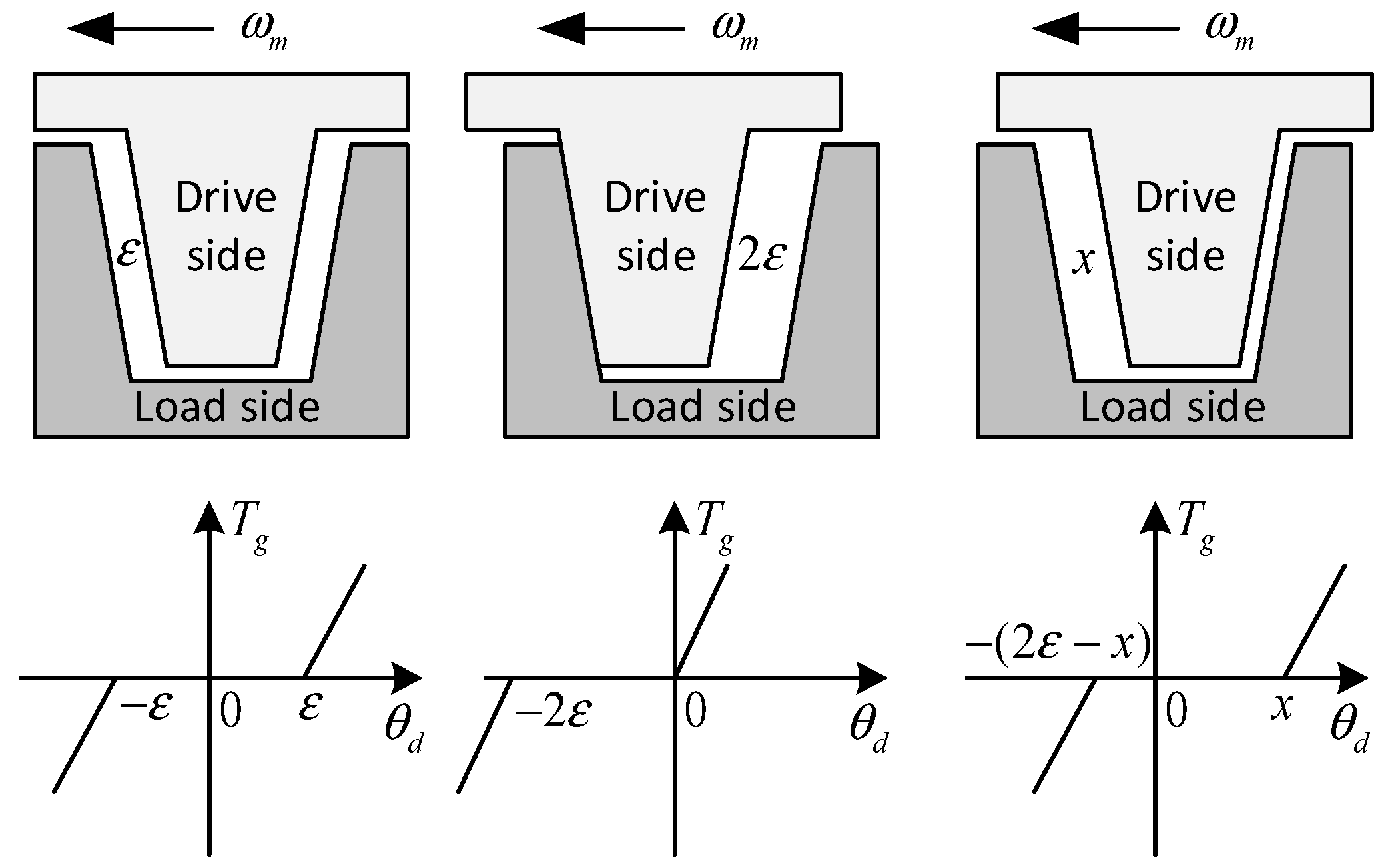
2.1. Gap Dead-zone Model

The dead-zone non-linear model of the gap delineates the torque transmission dynamics between the driving and driven wheels, accounting for elastic deformation due to rotational angle disparities. This model, unlike the hysteresis model, incorporates both positional and torque transmission aspects, aligning more closely with real-world motion conditions. Consequently, our study adopts the dead-zone model, represented mathematically in (1), where Tg signifies transmission shaft torque, K denotes stiffness coefficient, c represents damping coefficient, θm is motor side shaft rotation angle, θl is load side shaft rotation angle, and θd is the angle difference between drive side and load side that equals to θmθl. In addition, 2ε indicates gap angle amplitude. Figure 1 illustrates the input-output relationship of the dead-zone gap model, corresponding to (1).
T g = K ( θ m θ l ε ) + c ( θ ˙ m θ ˙ l ) 0 K ( θ m θ l ε ) + c ( θ ˙ m θ ˙ l ) θ m θ l > ε ε θ m θ l ε θ m θ l < ε
However, this relationship solely applies when the follower wheel resides centrally within the gap. In other positions, the curve shifts laterally, as depicted in Figure 2. Introducing the initial clearance as ε0, (1) undergoes revision to accommodate these variations.
T g = K ( θ m θ l ε 0 ) + c ( θ ˙ m θ ˙ l ) 0 K ( θ m θ l + 2 ε ε 0 ) + c ( θ ˙ m θ ˙ l ) θ m θ l > ε 0 ( 2 ε ε 0 ) θ m θ l ε 0 θ m θ l < ( 2 ε ε 0 )
In the equation, 0 ε 0 2 ε .

2.2. Gap Amplitude Identification

In gap identification, installing position sensors on both the drive motor and load sides is the most straightforward approach. However, practical constraints such as cost, installation complexity, and environmental considerations often preclude sensor placement on the load side. Consequently, only position data from the motor side is typically available. This section explores two methods for identifying gap amplitudes: one based on incremental torque pulses and the other on integrated velocity differences, as outlined in reference [6]. To assess identification accuracy, a comparison is made using position sensors on both sides, as depicted in Figure 3. The dotted line in the figure is the drive side rotor position. The measured gap value is found to be 0.03 rad (2ε = 1.72°).

2.2.1. Identification of Gap Amplitude Based on Incremental Torque Pulses

The identification method involves applying small torque pulses to the drive motor after positioning the system at zero, causing displacement while the load remains stationary. Subsequently, larger torque pulses are applied until the drive motor passes through the entire dead zone of the gap, ensuring that the energy of the torque pulse is insufficient to drive the load. When the feedback positions of the drive motor coincide on two occasions, it indicates traversal of the entire dead zone, corresponding to the gap value.
The experiment waveforms depicted in Figure 4 illustrate torque starting from 0.01 N·m, incrementing by 0.002 N·m iteratively. The dotted line displays the maximum value of rotor position. At a motor position of 0.027 rad, further increasing torque pulses yield negligible motor position changes. Thus, the identified gap amplitude is 0.027 rad, with a 10% identification error. However, this method faces challenges such as repetitive zero-point positioning, continuous trial and error of torque pulse amplitudes, and potential motion induction in the load.

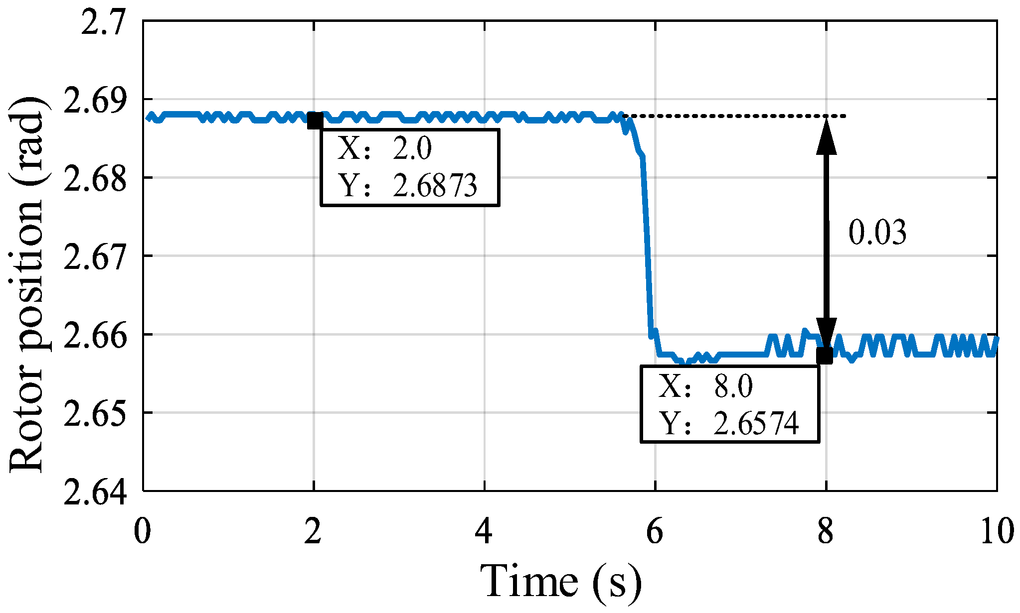
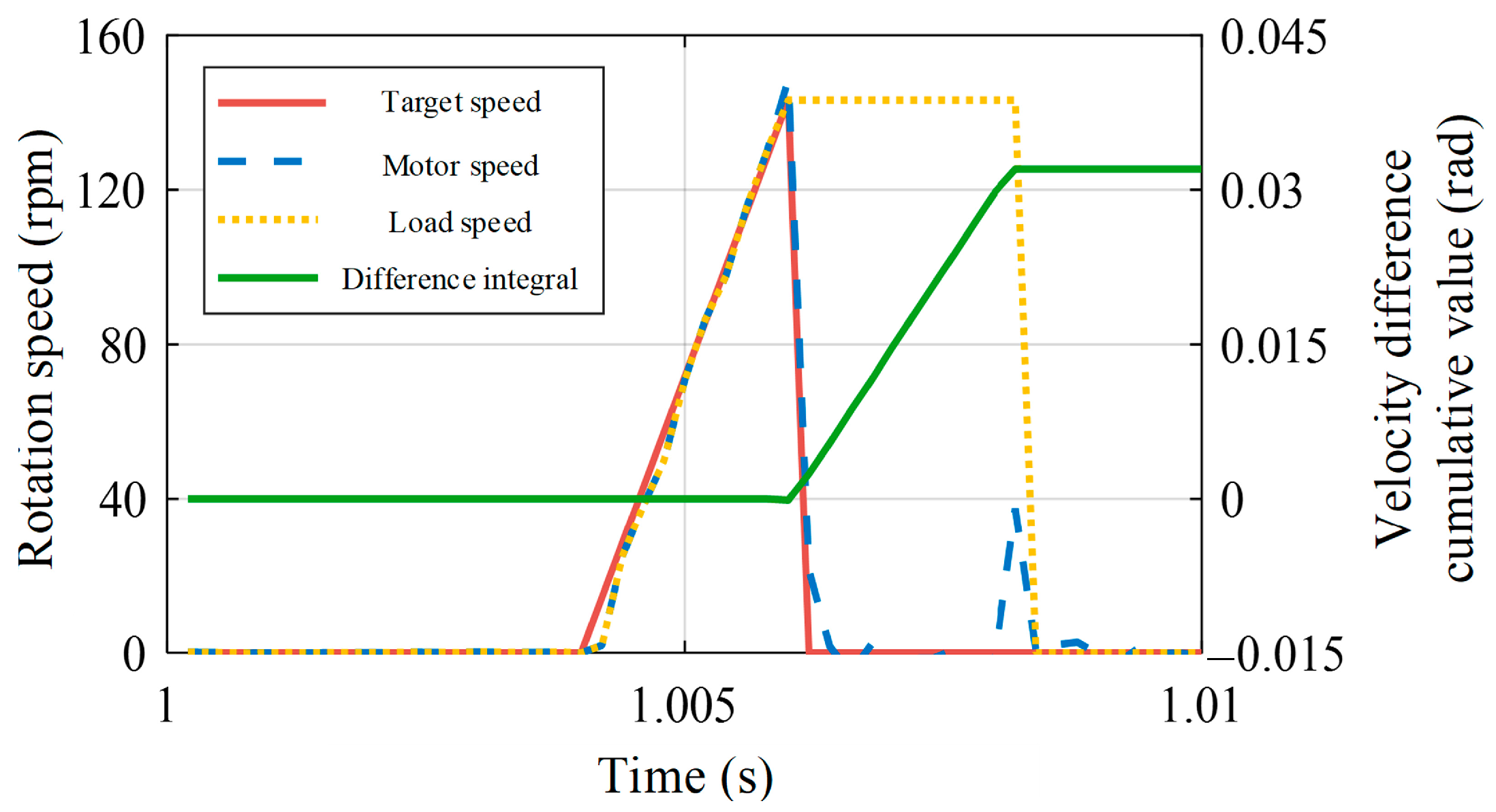
2.2.2. Gap Amplitude Identification Based on Velocity Difference Integration

This method employs a triangular speed signal where, upon reaching the maximum speed (ωmax), the speed abruptly shifts to 0, reversing acceleration and torque polarity. Consequently, the shaft traverses the gap’s dead zone. If the load’s inertia torque surpasses friction torque, it proceeds at ωl = ωmax until meshing with the other side. Gap amplitude is determined by integrating speed differences, with integration start and end times crucially determined by signal changes and collision-induced speed shifts on the drive motor side.
2 ε = t 1 t 2 [ ω l ( t ) ω m ( t ) ] d t
2 ε T s k 1 k 2 [ ω max ( k ) ω m ( k ) ]
Figure 5 illustrates the experimental waveform, yielding a speed difference integral of 0.032 rad. Since the gap measurement obtained above is 0.03 rad, this method has an identification error of 6.7%, demonstrating superior accuracy compared to the incremental torque pulse technique.

2.3. Impact of Two-Position Feedback Structures

In fully closed-loop servo control, the load-side position sensor enables direct feedback, facilitating high-precision positioning control. However, mechanical transmission components with significant rotational inertia lower the system’s natural frequency, often masked by expanding control system bandwidth. Non-linear gaps on the axis can induce limit-cycle oscillations, as depicted in Figure 6a, showing load-side position and speed responses oscillating symmetrically around a specified position. Figure 6b illustrates phase trajectory waveforms winding into closed curves, indicating limit-cycle oscillations.
Figure 6 illustrates the response of a fully closed-loop control system to a ramp input. In semi-closed-loop control, the drive motor’s position serves as feedback for the load-side position; however, this paper is concentrated on the fully closed-loop.

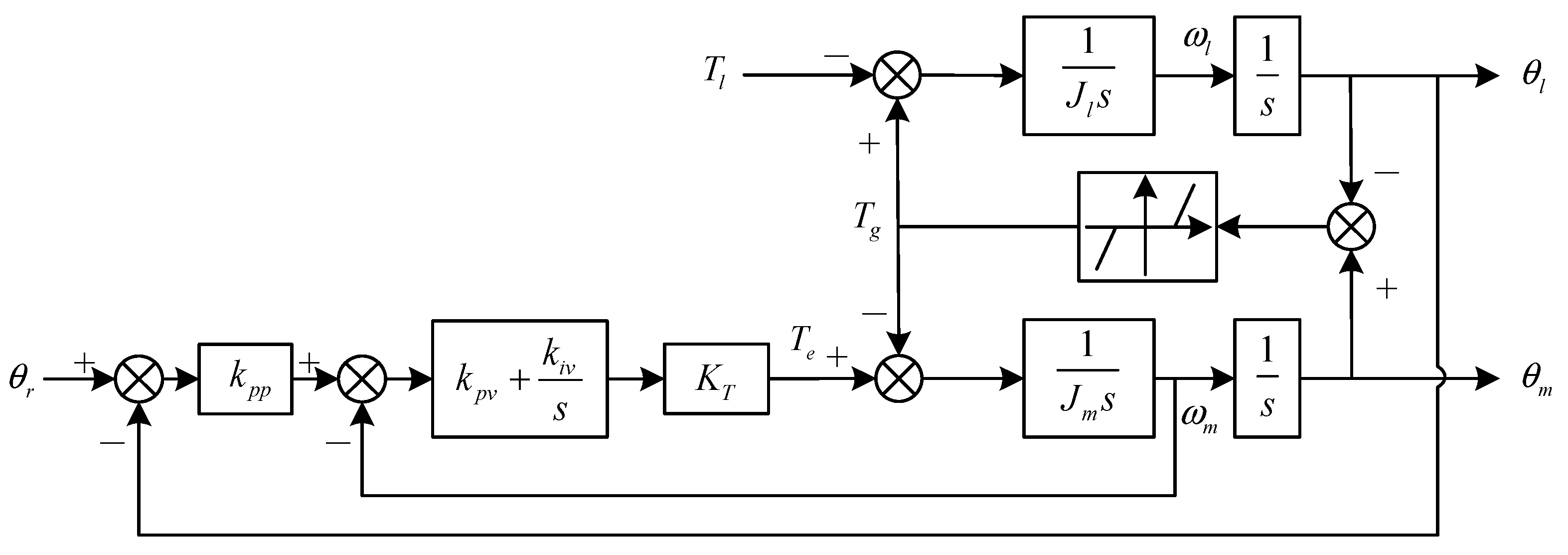
3. Under the Fully Closed-Loop Control Structure, Gap Nonlinearity Compensation Based on State Feedback

This section employs the describing function analysis method to examine the characteristics of limit-cycle oscillations arising from gaps. The method, introduced by P.J. Daniel, approximates the output of a nonlinear element subjected to a sinusoidal signal as a single harmonic component, facilitating the derivation of its frequency response, termed the describing function [12]. By assuming an initial gap value of ε0 = ε, as depicted in Figure 2, the system is treated as linearized, enabling the application of frequency-domain analysis techniques typically used in linear systems.

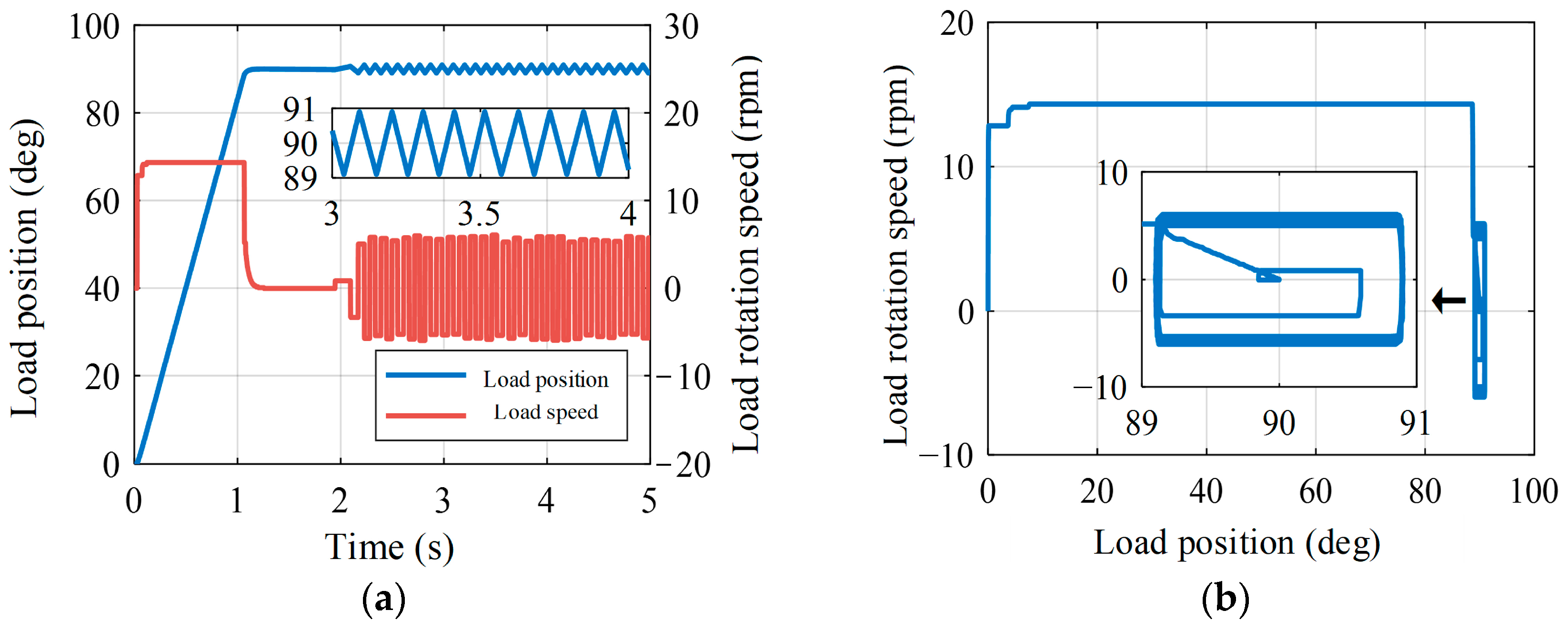
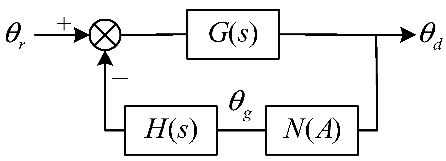
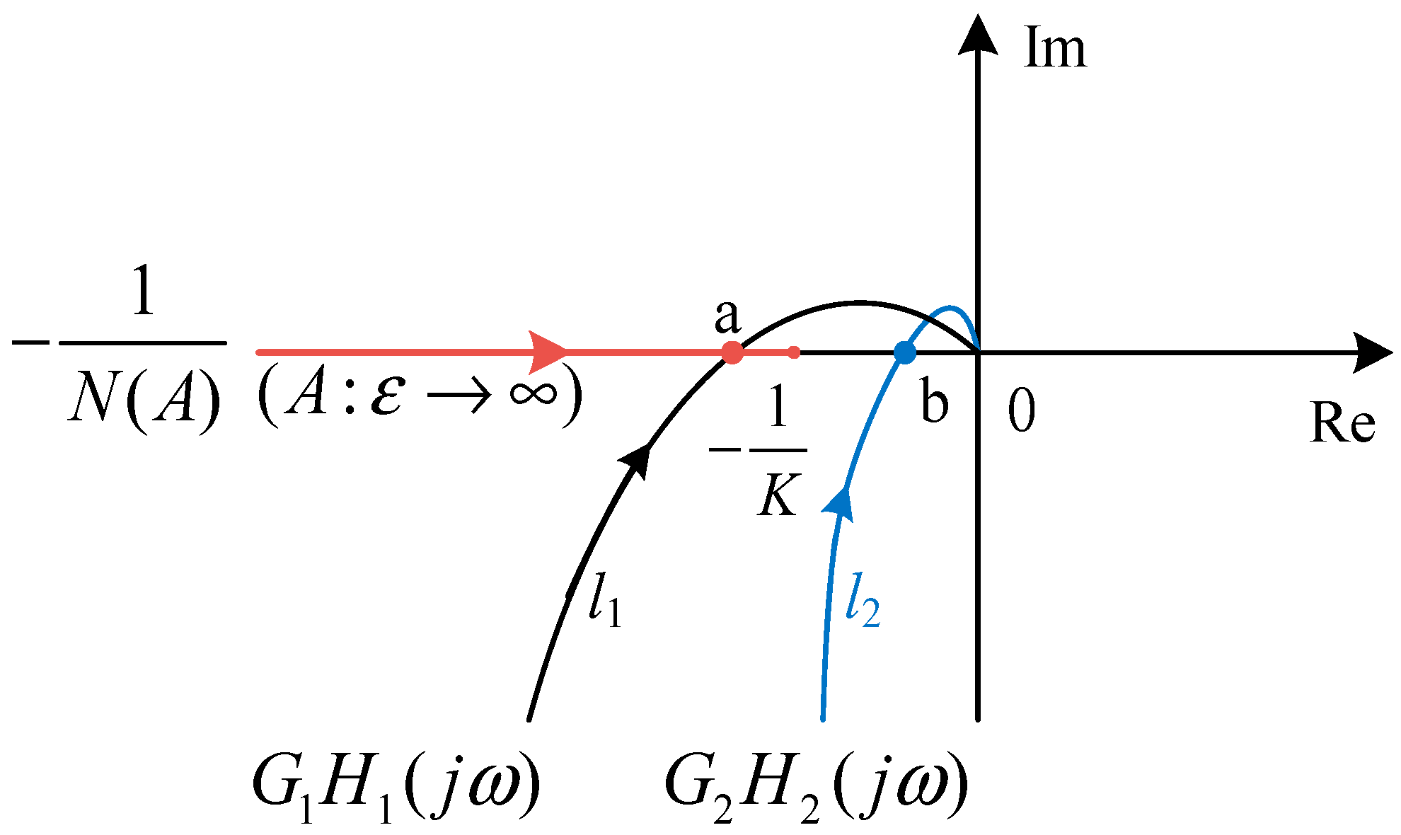
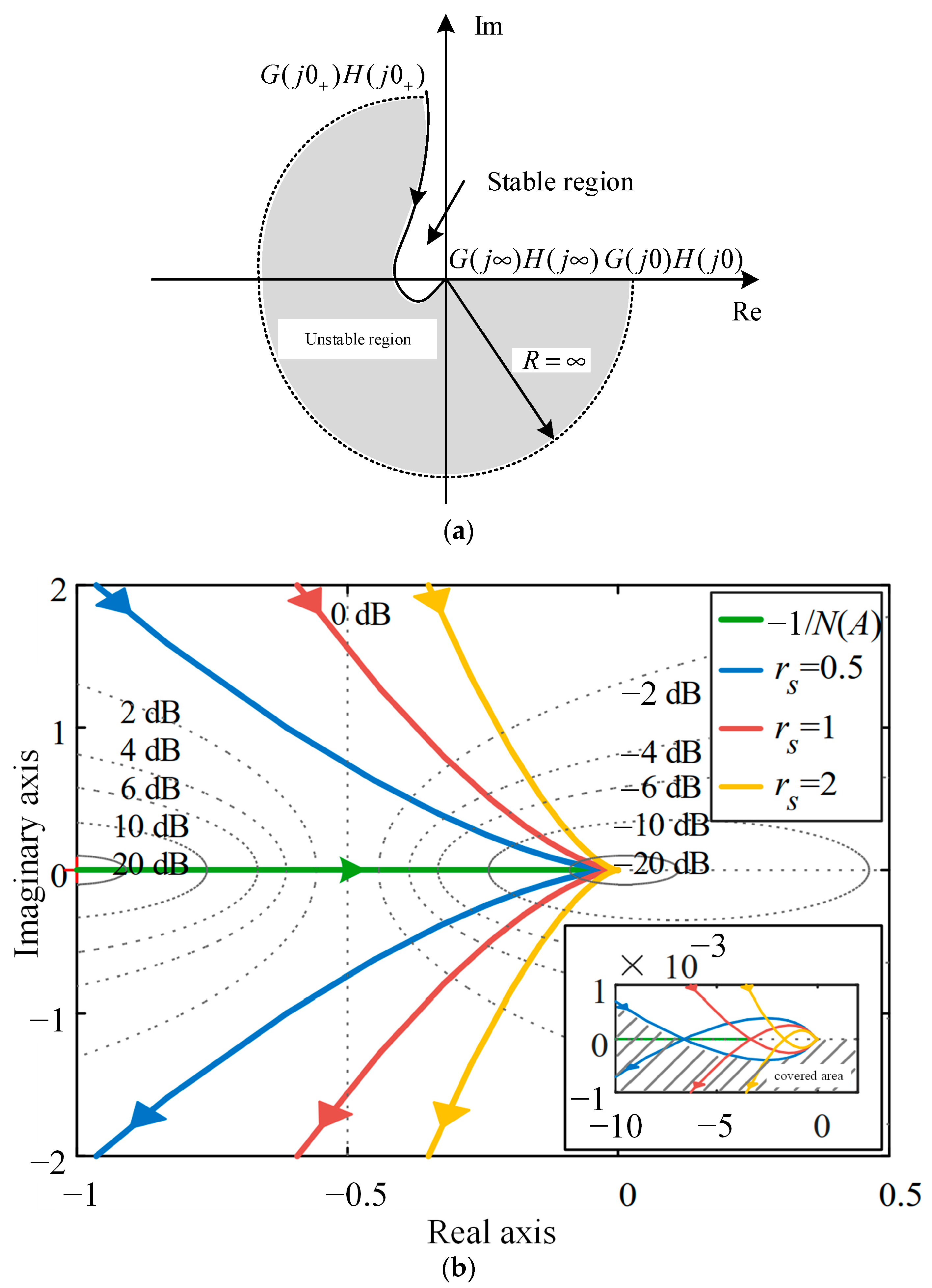
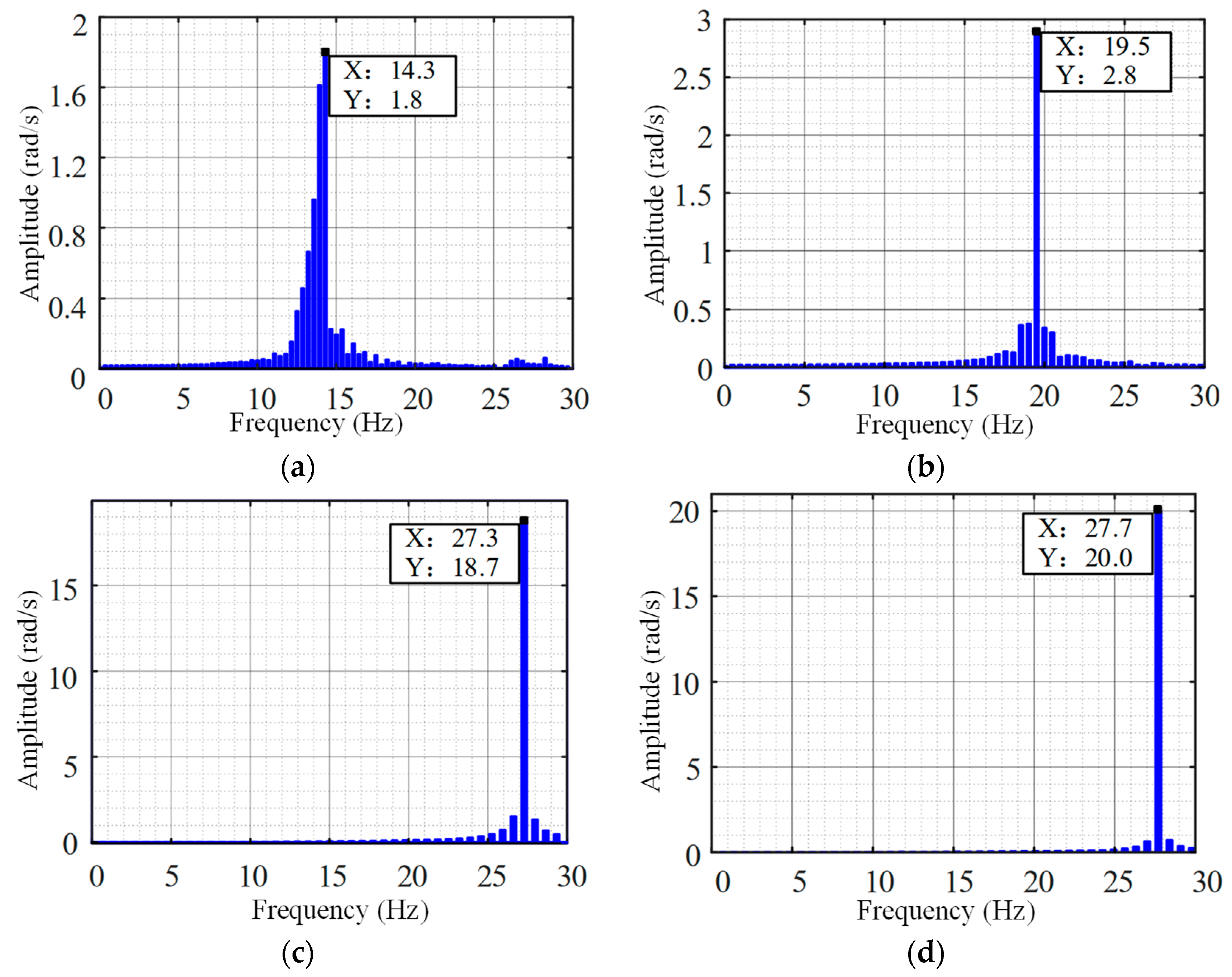
3.1. Analysis of Limit-Cycle Oscillation Mechanism

Triple-loop PI control is a prevalent method in industrial settings. In this control scheme, as depicted in Figure 7, the position loop utilizes proportional (P) control, while the velocity loop employs proportional-integral (PI) control. The current inner loop is simplified to unity. To facilitate describing function analysis, the control structure must undergo simplification into linear and nonlinear elements, as illustrated in Figure 8. Here, G(s) and H(s) represent linear elements, while N(A) signifies dead-zone nonlinearity. Additionally, θd denotes the difference between the drive-motor-side and the load-side positions, and θs represents the torque angle generating the transmission torque. Through derivation and classical nonlinear describing functions, the transfer function expressions can be derived.
G ( s ) = k p p ( k p v s + k i v ) K T J m s 3 + ( k p v s 2 + k i v s ) K T
H ( s ) = 1 k p p J l K T ( J m + J l ) s 3 + k p v s 2 K T + ( k p p k p v + k i v ) s K T + k p p k i v K T ( k p v s + k i v ) s 2
N ( A ) = 2 K π π 2 arcsin ε A ε A 1 ε A 2 , A ε
Applying the theorem of limit cycle existence, it is established that if, on the complex plane, the Nyquist trajectory G()H() corresponding to the linear link transfer function intersects with the trajectory of the negative reciprocal of the describing function of the nonlinear link −1/N(A), limit cycles exist within the system.
G ( j ω ) H ( j ω ) = 1 N ( A )
Hence, the system undergoes limit-cycle oscillations, where the crossing point signifies the oscillation frequency for the linear element and the amplitude for the nonlinear element. From the (7), the reciprocal of the describing function of the nonlinear element remains real. Consequently, the condition for the presence of intersection points for limit-cycle oscillations requires the imaginary part of G(H() to be zero, corresponding to determining the characteristic roots of the closed-loop transfer function. By deriving the expression for the imaginary part, as depicted in (10), the frequency of limit-cycle oscillations is determined as presented in (11). Given the negligible impact of the integral parameter of the velocity loop on limit-cycle oscillations [13], setting kiv = 0 and further simplification leads to the expression for the frequency of limit-cycle oscillations as provided in (12).
G ( s ) H ( s ) = 1 J l ( J m + J l ) s 3 + k p v s 2 K T + ( k p p k p v + k i v ) s K T + k p p k i v K T ( J m s 2 + k p v K T s + k i v K T ) s 3
Im [ G ( j ω ) H ( j ω ) ] = J l k p v K T ω 4 J m k p p k i v K T ω 2 + k p p k p v 2 K T 2 ω 2 + k p p k i v 2 K T 2 J l ( J m 2 ω 7 2 J m k i v K T ω 5 + k p v 2 K T 2 ω 5 + k i v 2 K T 2 ω 3 ) = 0
ω l c = P k p p k i v J m + k p p k p v 2 K T 2 J l k p v P = k p p 2 k i v 2 J m 2 2 k p p 2 k p v 2 k i v K T J m + k p p 2 k p v 4 K T 2 + 4 k p p k p v k i v 2 K T J l
ω l c = k p p k p v K T J l = r s ω A R F
In the equation, r s = k p p k p v K T K , the term “stiffness ratio” is employed to characterize the control stiffness of the system.
Variations in system stiffness ratios result in different limit-cycle frequencies. The earlier derived frequencies are based on necessary conditions for existence, but the absence of intersecting curves does not imply nonexistence. (7) shows that N(A) is a monotonic function, with its negative reciprocal range on the real axis from (∞, −1/K) when the limit value is substituted. In Figure 9, if the Nyquist curve of the linear portion is l1 and intersects at point a, a limit cycle exists; if it is l2 and its intersection point with the real axis lies outside the negative reciprocal range, further correction is required for the predicted frequency formula.
1 N ( ε ) = , 1 N ( ) = 1 K
The transfer function G(s)H(s) of the linear element, represented in the s-plane, forms a rational function with real coefficients, resulting in a closed-loop locus symmetric about the real axis. Thus, analyzing the semi-closed-loop locus is adequate for understanding its characteristics. With three poles at the origin and s = ρe, near which an infinitesimal quantity ρ and θ ∈ [0°, 90°] are considered, (15) can be derived. The locus initiates from G1(ρe) = G1(j0), creating an arc with an infinite radius and a central angle of −270°. Consequently, a counterclockwise arc, starting from the point G(j0+)H(j0+), is drawn with an infinite radius and a central angle of 270°, depicted by the dashed line in Figure 10a. By analyzing various values of rs, the intersection of the linear element’s Nyquist locus and the reciprocal curve of the nonlinear element is plotted, as shown in Figure 10b.
G 1 ( s ) = G ( s ) H ( s ) s 3 = 1 J l ( J m + J l ) s 3 + k p v s 2 K T + ( k p p k p v + k i v ) s K T + k p p k i v K T ( J m s 2 + k p v K T s + k i v K T )
G ( s ) H ( s ) | s = ρ e j θ e j ( 1 ρ 3 e j 3 θ + G 1 ( ρ e j θ ) ) = e j ( 3 θ + G 1 ( j 0 ) )
In the complex plane, the region bounded by G()H() delineates the unstable region, while the unbounded area denotes stability. Figure 10b illustrates the shaded region as the unstable region for rs = 0.5. According to the stability criterion for nonlinear systems:
(1) If the linear loop curve G()H() fails to intersect the negative reciprocal curve of the nonlinear loop, 1/N(A), the system is stable provided G()H() does not enclose −1/N(A); otherwise, it is unstable.
(2) If G()H() intersects −1/N(A) at the intersection point, the stability or instability of oscillations depends on the transition of −1/N(A) from unstable to stable as amplitude A increases, indicating stability, or from stable to unstable, indicating instability.
For rs < 1, the intersection of the two curves occurs, where −1/N(A) transitions from an unstable to a stable region as A increases, indicating stable periodic oscillations. At rs = 1, the system reaches a critical state, oscillating at the anti-resonance frequency ωARF. Conversely, for rs > 1, the absence of intersection results in the envelopment of the entire −1/N(A) curve, signifying system instability. However, the inherent oscillatory characteristics of the mechanical system led to an increase in the limit-cycle frequency to ωARF, constraining oscillations to persist at this frequency. Consequently, the prediction formula for the limit-cycle oscillation frequency undergoing modification is as follows:
ω l c = r s ω A R F ω A R F 0 < r s < 1 r s 1
Experimental validation of limit-cycle frequency prediction was performed, necessitating modifications to the experimental setup to mitigate excessive resonant frequencies. Detailed parameters for these modifications are outlined in Table 1.
The PI controller parameters were rectified by combining the zero-pole pair cancellation and the controller step-down method.
Figure 11 illustrates the FFT analysis of load speed at varying stiffness ratios, achieved primarily through adjusting the position loop gain. For kpp = 26 and rs = 0.55, the calculated oscillation frequency is 16.3 Hz, slightly deviating by 2 Hz from the actual FFT analysis result of 14.3 Hz. At kpp = 35 and rs = 0.625, the calculated frequency is 18.6 Hz, showing a 1.1 Hz error compared to the actual FFT analysis output of 19.5 Hz. Similarly, with kpp = 88 and rs = 1, the calculated frequency is 29.7 Hz, deviating by 2.4 Hz from the actual output of 27.3 Hz. Even at kpp = 130 with rs = 1.2, the calculated frequency remains at 29 Hz, while the actual output is 27.7 Hz, indicating oscillation at the anti-resonance frequency ωARF. Increasing proportional gain augments control stiffness, intensifying limit-cycle oscillations with larger amplitudes, consistent with theoretical analysis and validating the predictive formula.
Figure 11b and Figure 12 display FFT analyses of load velocity at gap amplitudes of 0.02 rad, 0.04 rad, and 0.1 rad, respectively. Comparative examination reveals a consistent oscillation frequency of approximately 19.6 Hz across all three amplitude sets, signifying that those alterations in gap amplitude do not influence oscillation frequency within a stable oscillatory region. Furthermore, oscillation amplitudes were documented at 2.8, 5.8, and 14.6 rad/s, demonstrating a pattern of geometric proportionate growth consistent with theoretical analysis.

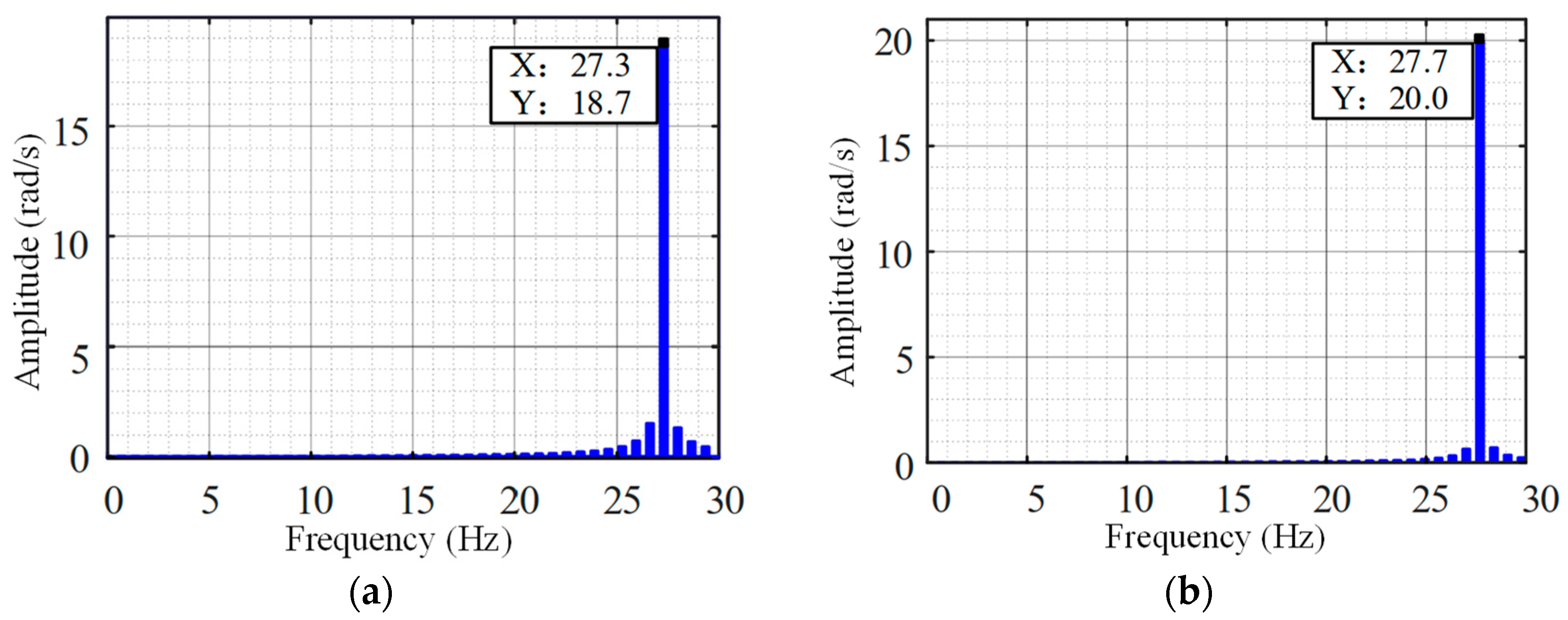
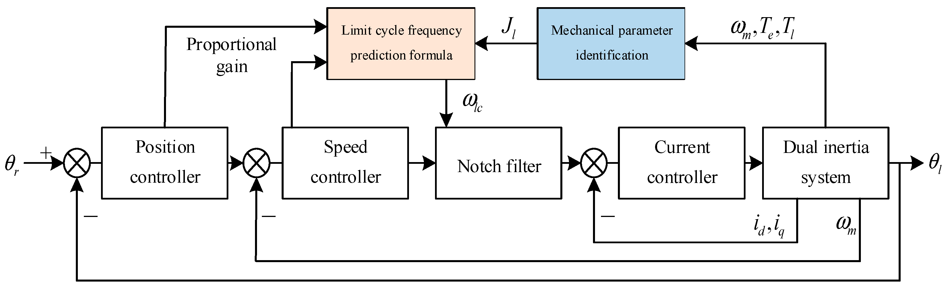
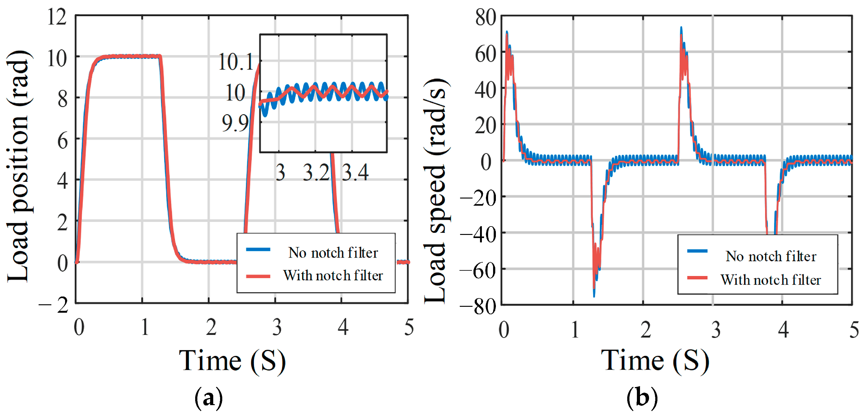
3.2. Suppression of Limit-Cycle Oscillations Using Notch Filters

This study explores notch filters shown in Figure 13 as a potential solution for suppressing oscillations by attenuating the amplitude at the resonant frequency. Simulation experiments utilize the predicted limit-cycle frequency from (16). Figure 14 illustrates a modest reduction in load-speed amplitude and a decrease in oscillation frequency. However, complete suppression remains elusive, as evidenced by the persistent oscillations.
From the above FFT analysis, it can be seen that in addition to the limit-ring oscillation frequency, there are other harmonics at unpredictable frequencies, and an adaptive multi-frequency trap is required if the filter continues to be applied. In order to avoid complex design, the main reason for the formation of gap resonance is further considered: due to the dead band characteristics of the gap, the system axial torque changes abruptly to 0 in the tooth gap stage, while the electromagnetic torque remains constant, allowing the motor to continue to accelerate, which ultimately leads to impulses and oscillations, as shown in Figure 15. Therefore, reasonable compensation of electromagnetic torque is the key to solving the gap limit-ring oscillation.

3.3. Suppression of Limit-Cycle Oscillations Based on State Feedback

3.3.1. Structural Design

A composite system formed by serially connecting an nth-order integrative inverse system with the original system is termed a pseudo-linear system. Effective control over this system necessitates designing an external control network based on it, involving determining the control structure and parameters per the control requirements. Two commonly employed methods for external loop control are state-feedback control and asymptotic tracking control.
State feedback is employed in this section to achieve full closed-loop oscillation suppression. By compensating the q-axis current, electromagnetic torque during tooth clearance separation is reduced. This approach mitigates significant speed differences between the two sides, diminishes impacts, and suppresses limit-cycle oscillations, approximating the system to a single-inertia linear system. The control structure, depicted in Figure 16, selects the position difference between the two sides and its first derivative as state variables. This design, derived from multiple simulations and experimental trials, balances complexity and control effectiveness. To address noise amplification from direct differentiation, a first-order low-pass filter with a cutoff frequency of 500 rad/s is utilized.

3.3.2. Design of Feedback Parameters

The feedback parameter design philosophy employs pole placement methodology to reduce system order based on the current nonlinear system’s transfer function. This approach effectively transforms a dual-inertia system into a single-inertia system, consequently alleviating the effects of backlash nonlinearity. The transfer function between the load position and the set position is as follows:
θ l θ r = k p p ( k i v + k p v s ) K T N ( A ) D ( s ) D ( s ) = J m J l s 5 + ( k p v J l K T k 2 J l K T ) s 4 + [ ( J l + J m ) N ( A ) + k i v J l K T k 1 J l K T ] s 3 + k p v K T N ( A ) s 2 [ k i v K T N ( A ) + k p p k p v K T N ( A ) ] s + k p p k i v K T N ( A )
In practical control engineering, higher-order systems typically necessitate rapid dynamic responses, sufficient damping, and mitigation of nonlinear influences on performance. To achieve these requirements, adjustments to the system’s gain are often made to ensure the presence of a pair of closed-loop conjugate dominant poles. Considering the inclusion of a closed-loop zero in the transfer function, the pole configuration is carefully designed to encompass a pair of dominant conjugate poles, a pair of non-dominant conjugate poles, and an additional pole employed for canceling the closed-loop zero. This formulation establishes the standard form of the characteristic equation:
( s 2 + 2 ζ 1 ω 1 s + ω 1 2 ) ( s 2 + 2 ζ 2 ω 2 s + ω 2 2 ) ( s + ω 3 ) = 0
The formula incorporates damping factors (ζ₁ and ζ₂) and oscillation frequencies (ω₁, ω₂, and ω₃), representing poles correspondingly.
s 1 , 2 = ζ 1 ω 1 ± ω 1 ζ 1 2 1 s 3 , 4 = ζ 2 ω 2 ± ω 2 ζ 2 2 1   s 5 = ω 3 = k i v / k p v ( a ) ( b ) ( c )
For this analysis, the dominant poles s1 and s2 are chosen, ensuring the condition ζ2ω2 ≥ 5ζ1ω1, as per the definition of dominant poles.
By equating the coefficients of (17) and (18), a system of equations is obtained comprising eleven parameters: feedback coefficients k1 and k2, controller parameters kpp, kpv, kiv, pole parameters ζ1, ζ2, ω1, ω2, ω3, and the nonlinear parameter N(A). Among these, four pole parameters can be arbitrarily set, while the remaining seven are determined from (8), (19) (c), and (20). The expressions for these parameters are provided in (21).
k p v K T k 2 K T J m = 2 ζ 1 ω 1 + 2 ζ 2 ω 2 + ω 3 ( a ) ( J l + J m ) N ( A ) + k i v J l K T k 1 J l K T J m J l = ω 1 2 + ω 2 2 + 4 ζ 1 ζ 2 ω 1 ω 2 + 2 ζ 1 ω 1 ω 3 + 2 ζ 2 ω 2 ω 3 ( b ) k p v K T N ( A ) J m J l = ω 1 2 ω 3 + ω 2 2 ω 3 + 4 ζ 1 ζ 2 ω 1 ω 2 ω 3 + 2 ζ 1 ω 1 ω 2 2 + 2 ζ 2 ω 1 2 ω 2 ( c ) k i v K T N ( A ) + k p p k p v K T N ( A ) J m J l = ω 1 2 ω 2 2 + 2 ζ 1 ω 1 ω 2 2 ω 3 + 2 ζ 2 ω 1 2 ω 2 ω 3 ( d ) k p p k i v K T N ( A ) J m J l = ω 1 2 ω 2 2 ω 3 ( e )
k i v = 0 k p v = 2 ( ζ 1 ω 2 + ζ 2 ω 1 ) ( J m J l ) ω 3 = 0 k p p = ω 1 ω 2 2 ( ζ 1 ω 2 + ζ 2 ω 1 ) k 1 = ω 1 ω 2 ( J m + J l ) J m J l J l K T J m ( ω 1 2 + ω 2 2 + 4 ζ 1 ζ 2 ω 1 ω 2 ) K T k 2 = 2 ( ζ 1 ω 2 + ζ 2 ω 1 ) J m J l K T 2 J m ( ζ 1 ω 1 + ζ 2 ω 2 ) K T N ( A ) = ω 1 ω 2 ( J m + J l ) J m J l
The positional loop gain, kpp, is independent of other mechanical parameters, solely determined by pole configuration parameters. Notably, kiv and ω3 are deliberately set to zero. This decision is based on the proximity of closely spaced zeros and poles to the imaginary axis, where their combined influence cannot be discounted. Thus, by nullifying kiv, a zero and a pole are effectively eliminated, leading to the revision of the system transfer function from (17) to (22).
θ l θ r = k p p k p v K T N ( A ) D ( s ) D ( s ) = J m J l s 4 + ( k p v J l K T k 2 J l K T ) s 3 + [ ( J l + J m ) N ( A ) k 1 J l K T ] s 2 + k p v K T N ( A ) s k p p k p v K T N ( A )

3.3.3. Steady-State Error

In motor control, the common methods to reduce steady-state error are feed-forward control, observer control, and PID-optimal control. In this paper, PID optimization design incorporating state feedback is used, which is suitable for engineering applications.
State-feedback control enhances system dynamic performance but does not guarantee zero steady-state error tracking for polynomial inputs like (23) [10]. Examination of this system as a pseudo-linear system indicates that its open-loop transfer function resembles a type-zero system, thus demonstrating error even under step input conditions.
r ( t ) = i = 1 l P i t i
lim t e ( t ) = lim t [ r ( t ) y ( t ) ] = 0
This project employs qualitative simulation analysis to assess the steady-state error in nonlinear systems, as direct computation of static error is unfeasible. By altering one parameter at a time while keeping others constant, steady-state errors are observed under various conditions, as illustrated in Figure 17. The analysis reveals that the steady-state static error is directly linked to the feedback coefficient k1 and the gap amplitude 2ϵ, while inversely related to the proportional coefficients of the position loop kpp and velocity loop kpv. Notably, the steady-state error remains unaffected by the set position signal θr and the feedback coefficient k2. The derived static error formula, presented in (25), is consistent with the simulation findings. Additionally, the original control parameters are documented in Table 2.
θ r θ l = e = k 1 ( θ m θ l ) k p p k p v
In no-load simulations, θmθl = −ϵ, but under load, Tg and Tl affect the state-feedback compensation current via (1).
i c o m p = k 1 ( θ m θ l ) T l K T = k 1 T l K + ε T l K T = k 1 T l K T ( T l / K + ε ) k 1 T l K + ε ε
(24) is revised to
e = k 1 ( T l / K + ε ) T l / K T k p p k p v
The examination of (25) and (27) reveals that adjusting control parameters can mitigate steady-state error. However, excessive modifications may trigger resonance, as depicted in Figure 17h. Hence, implementing steady-state error compensation at the specified terminal offers a safer alternative compared to extensive alterations of initially designed control parameters.

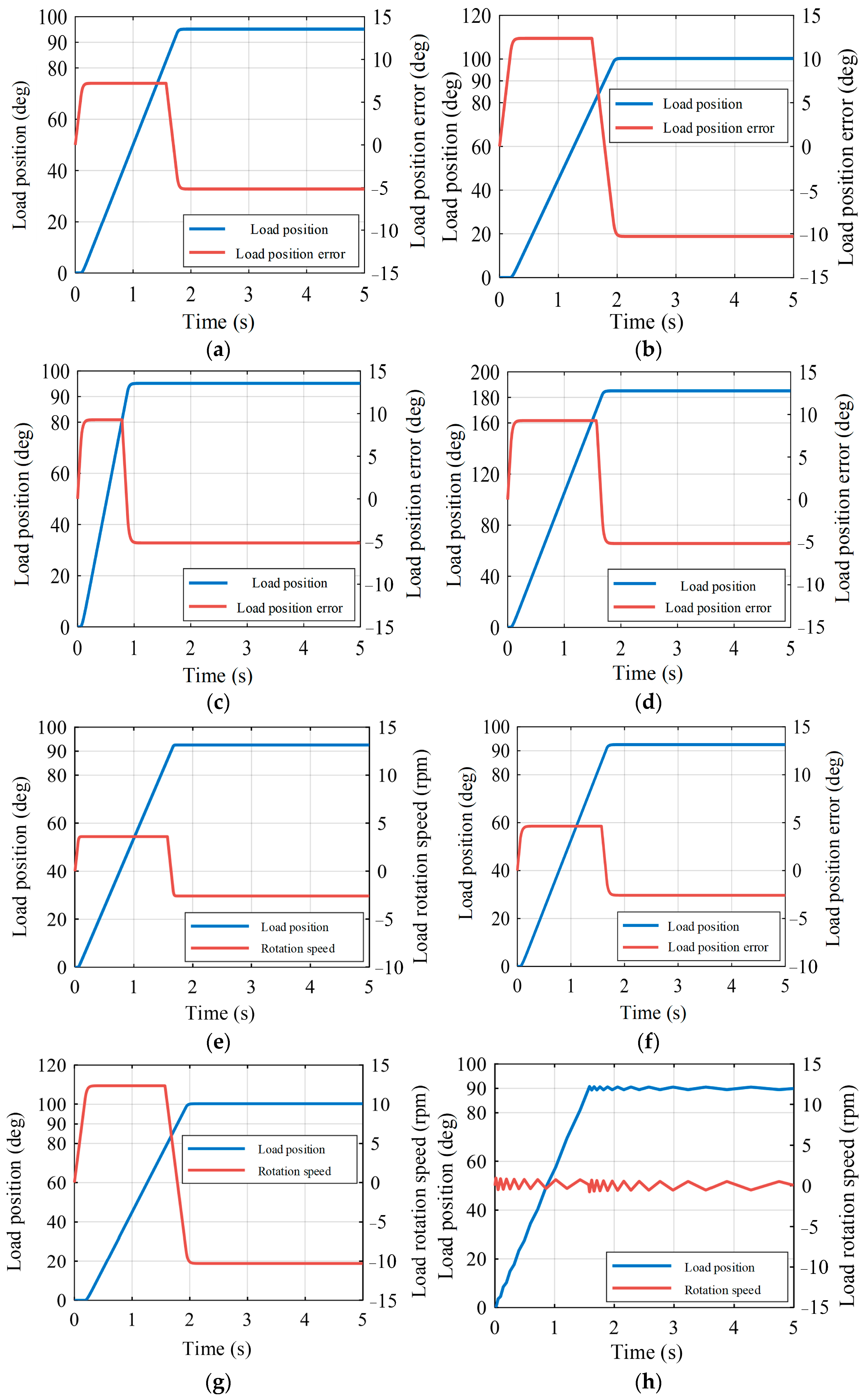
4. Simulation Validation

A dual-inertia servo system model was built in MATLAB/Simulink for simulation verification. The simulation affirms the state-feedback algorithm’s success in quelling limit-cycle oscillations, utilizing mechanical parameters consistent with the experimental platform in Section 5. Corresponding parameters for mitigating these oscillations align with those outlined in Table 2. Specifically, a clamped-ramp position signal of 90° is employed for assessment.

4.1. Comparison between PI Control and State-Feedback Control

Figure 18 illustrates load position and velocity responses within a closed-loop control framework employing a dual-inertia system with backlash. Both PI control and state-feedback control were applied using identical simulation parameters. Notably, Figure 18b shows that state-feedback control effectively suppresses periodic oscillations, maintaining dynamic characteristics similar to those observed under PI control. This underscores the capacity of state-feedback control to mitigate limit-cycle resonance by strategically placing poles, consequently improving positioning accuracy.

4.2. Robustness under Varying System Parameters

During system operation, sudden variations in load inertia and backlash amplitude due to wear are common scenarios. To assess the robustness of state-feedback control across different system parameters, simulations were conducted with parameter variations.
Initially, simulations were performed with the backlash amplitude altered to 0.06 rad. A comparison between Figure 18a and Figure 19a reveals that PI control fails to suppress oscillations, with an increase in backlash amplitude resulting in larger oscillation amplitudes, consistent with Section 3.1 analysis. In contrast, state-feedback control effectively suppresses limit-cycle oscillations, as demonstrated in Figure 19b.
The simulation was then carried out under the condition of only changing the load inertia to 2Jl. As shown in Figure 20, the state-feedback control still had a good control effect. The simulation shows that the method has parametric robustness.

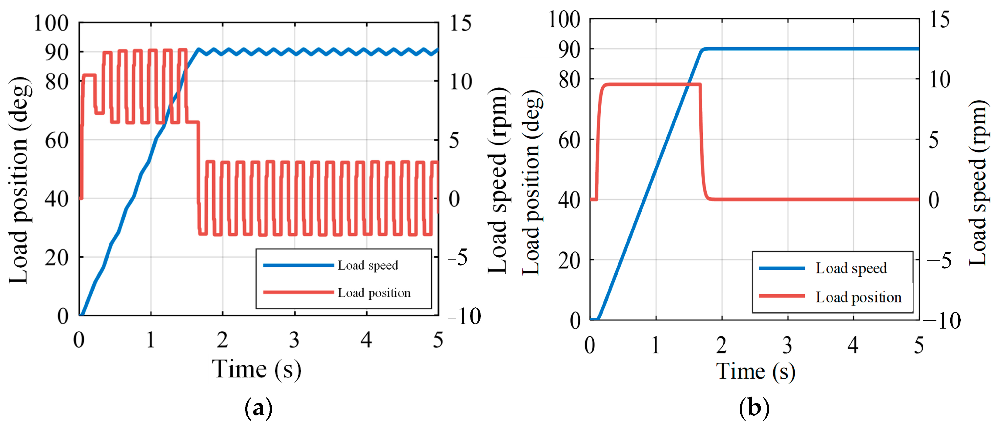
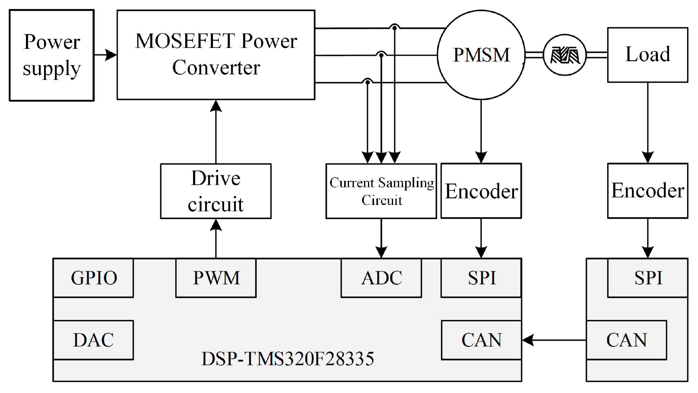
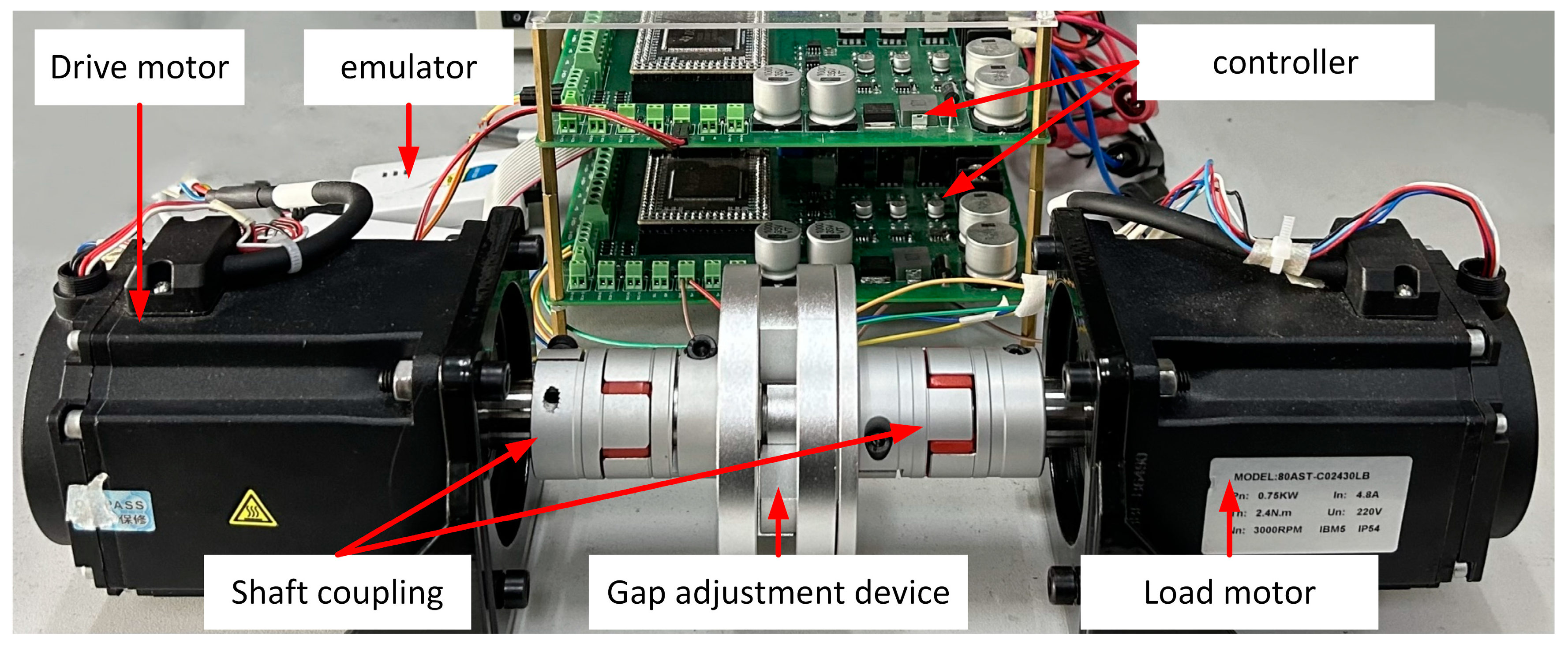
5. Experimental Validation

Figure 21 shows the block diagram of the hardware circuit structure of the dual-inertia servo system. The microprocessor is a Texas Instruments DSPTMS320F28335 chip, through the sampling module to get the motor three-phase current, according to the real-time position feedback from the AS5047P absolute encoder, calculate and update the duty cycle of the ePWM output to drive the motor rotation. The load-side controller is the same as the driver side, and the two transmit position signals in both directions through CAN communication.
The experimental platform used in this paper is shown in Figure 22.
Two M02430LBX motors were employed to construct the pair drag experimental platform, and the motor parameters are presented in Table 3.
The initial validation phase assessed steady-state error predictions, with results detailed in Figure 23 and Table 4. Four sets of parameters have been analyzed. Twenty percent of the rated load was used to simulate a typical application environment. Both theoretical and experimental steady-state errors closely matched. Transient process analysis, as shown in Figure 23b,c, revealed minor oscillations attributed to impact effects from clearance device engagement under no-load conditions.
Based on the theoretical and experimental static differences in Table 4, the absolute errors of the four sets of parameters can be calculated. The errors ranged from 1.5% to 15.3%, with the highest being 15.3% and the lowest 1.5%. During the transient process depicted in Figure 23b,c, minor oscillations occurred, attributed to impacts from the engagement of the clearance device under no-load conditions.
Experimental tests under no-load conditions evaluated system positioning accuracy using proportional control and state-feedback control. Figure 24a,b shows position and speed response waveforms, respectively. With PI control, periodic oscillations occurred with an amplitude of ±4.8°, eliminated by state-feedback compensation, improving steady-state performance. Additionally, state-feedback control reduced the maximum speed to 101.4 rpm from 141.1 rpm under PI control, minimizing system impact. Figure 24c depicts phase trajectories for both methods, confirming algorithm effectiveness.
Figure 25 shows the dynamic response of the system at 20% of the rated load, and it can be seen that the state-feedback compensation strategy is also applicable for the loaded case. Compared to the no-load response shown in Figure 24b, loading stabilizes the system to a certain extent and the velocity shock is further reduced to 56.4 rpm, but this also results in a slower dynamic response at the load position.

6. Conclusions

This paper presents a nonlinear dead-zone model with initial values and two methods for amplitude identification: incremental torque and speed difference integration, with the latter showing superior accuracy at just a 6.7% error. Moreover, this paper explores the structural characteristics of fully closed-loop control for dual-inertia systems. In the full-closed loop, the describing function method analyzes limit-cycle oscillations, finding the notch filter ineffective in suppressing oscillations induced by dead-zone nonlinearity. It identifies excessive electromagnetic torque causing abrupt speed changes as the core reason for oscillation and proposes a state-feedback compensation strategy, reducing the dual-inertia system to a single-inertia system through pole placement. Experimental results confirm the elimination of limit-cycle oscillations and reduced system shocks, with maximum impact speed under no-load conditions using the state-feedback compensation strategy being 28% lower than that under PI control.
In terms of future work, since the describing function method used in this paper can only study the frequency response characteristics, it cannot describe the time response. In addition, the describing function method only considers the case of the initial value of the gap ε0 = ε. Therefore, the describing function containing the initial value can be further derived and subsequently applied.

Author Contributions

Conceptualization and methodology, B.W. and R.J.; simulation, B.W. and C.Z.; validation and experiment, B.W. and H.Y.; writing, B.W. and R.J.; review and editing, R.J. and R.M.S.; supervision, K.L.; funding acquisition, W.H. All authors have read and agreed to the published version of the manuscript.

Funding

This research received no external funding.

Data Availability Statement

The original contributions presented in the study are included in the article, further inquires can be directed to the corresponding author.

Conflicts of Interest

The authors declare no conflict of interest.

References

  1. Zhao, Z.; Lin, S.; Zhu, D.; Wen, G. Vibration Control of a Riser-Vessel System Subject to Input Backlash and Extraneous Disturbances. IEEE Trans. Circuits Syst. II Express Briefs 2020, 67, 516–520. [Google Scholar] [CrossRef]
  2. Zhou, Z.; Guo, R. A Disturbance-Observer-Based Feedforward-Feedback Control Strategy for Driveline Launch Oscillation of Hybrid Electric Vehicles Considering Nonlinear Backlash. IEEE Trans. Veh. Technol. 2022, 71, 3727–3736. [Google Scholar] [CrossRef]
  3. Wang, C. Research on Mechanical Parameter Identification and Oscillation Suppression Techniques in Servo Drive Systems; Harbin Institute of Technology: Harbin, China, 2018. [Google Scholar]
  4. Hao, Q.; Li, G.; Ooi, B.T. Approximate model and low-order harmonic reduction for high-voltage direct current tap based on series single-phase modular multilevel converter. IET Gener. Transm. Distrib. 2013, 7, 1046–1054. [Google Scholar] [CrossRef]
  5. Reddy, P.; Shahbakhti, M.; Ravichandran, M.; Doering, J. Real-Time Estimation of Backlash Size in Automotive Drivetrains. IEEE/ASME Trans. Mechatron. 2022, 27, 3362–3372. [Google Scholar] [CrossRef]
  6. Yang, M.; Tang, S.; Tan, J.; Xu, D. Study of On-line Backlash Identification for PMSM Servo System. In Proceedings of the Annual Conference of the IEEE Industrial Electronics Society, Montreal, QC, Canada, 25–28 October 2012; pp. 2036–2042. [Google Scholar]
  7. Ahmad, N.J.; Ebraheem, H.K.; Alnaser, M.J.; Alostath, J.M. Adaptive Control of a DC Motor with Uncertain Deadzone Nonlinearity at the Input. In Proceedings of the Chinese Control and Decision Conference (CCDC), Mianyang, China, 23–25 May 2011; pp. 4295–4299. [Google Scholar]
  8. Shi, Z.; Zuo, Z. Backstepping Control for Gear Transmission Servo Systems with Backlash Nonlinearity. IEEE Trans. Autom. Sci. Eng. 2015, 12, 752–757. [Google Scholar] [CrossRef]
  9. Omisore, O.M.; Han, S.P.; Ren, L.X.; Wang, G.S.; Ou, F.L.; Li, H.; Wang, L. Towards Characterization and Adaptive Compensation of Backlash in a Novel Robotic Catheter System for Cardiovascular Interventions. IEEE Trans. Biomed. Circuits Syst. 2018, 12, 824–838. [Google Scholar] [CrossRef]
  10. Chen, Y.; Liu, Z.; Chen, C.L.; Zhang, Y. Fuzzy Control of Switched Systems with Unknown Backlash and Nonconstant Control Gain: A Parameterized Smooth Inverse. IEEE Trans. Fuzzy Syst. 2022, 30, 4876–4890. [Google Scholar] [CrossRef]
  11. Yang, M.; Wang, C.; Xu, D.; Zheng, W.; Lang, X. Shaft Torque Limiting Control Using Shaft Torque Compensator for Two-Inertia Elastic System with Backlash. IEEE/ASME Trans. Mechatron. 2016, 21, 2902–2911. [Google Scholar] [CrossRef]
  12. Bai, C.; Yin, Z.; Li, T.; Zhang, Y.; Yuan, D.; Zhang, P. Backstepping Control Collaborative Shaft Torque Observer for Limit Cycle Oscillation Suppression of Fully Closed-Loop Gear Transmission Servo System. IEEE Trans Power Electron. 2024, 39, 4513–4526. [Google Scholar] [CrossRef]
  13. Ghaffari, A.; Mohammadiasl, E. Calculating the Frequency of Oscillation for Servo Axes Distressed by Clearance or Preloading. IEEE/ASME Trans. Mechatron. 2013, 18, 922–931. [Google Scholar] [CrossRef]
Figure 1. Dead band model of gaps.
Energies 17 03582 g001
Figure 2. Gap dead-zone model with ini.
Energies 17 03582 g002
Figure 3. Experimental confirmation of gap amplitude.
Energies 17 03582 g003
Figure 4. Gap amplitude identification based on incremental torque pulses.
Energies 17 03582 g004
Figure 5. Gap amplitude identification based on velocity difference integration.
Energies 17 03582 g005
Figure 6. Response of a fully closed-loop control system to a ramp input: (a) Response of load position and speed; (b) Phase trajectory.
Energies 17 03582 g006
Figure 7. Block diagram of a dual-mass system with PI control.
Energies 17 03582 g007
Figure 8. Simplified control block diagram of dual inertia system with gap.
Energies 17 03582 g008
Figure 9. Gap deadband negative inverse descriptive function.
Energies 17 03582 g009
Figure 10. The case where a linear link Nyquist curve intersects a negative inverse curve: (a) Schematic diagram of the semi-closed curve; (b) Intersection at different stiffnesses.
Energies 17 03582 g010
Figure 11. Limit-ring oscillation frequency when stiffness varies (2ε = 0.02 rad): (a) rs = 0.55; (b) rs = 0.625; (c) rs = 1; (d) rs = 1.2.
Energies 17 03582 g011
Figure 12. Oscillation frequency of limit cycles at different gap intervals: (a) 2ε = 0.04 rad; (b) 2ε = 0.1 rad.
Energies 17 03582 g012
Figure 13. Resonance suppression based on notch filters.
Energies 17 03582 g013
Figure 14. Load response of the system with gap using a notch filter: (a) load position; (b) load speed.
Energies 17 03582 g014
Figure 15. Analysis of the physical causes leading to clearance limit-cycle oscillations: (a) torque response; (b) speed response.
Energies 17 03582 g015
Figure 16. Resonance suppression based on state feedback.
Energies 17 03582 g016
Figure 17. Steady-state error under different system parameters: (a) raw steady-state error; (b) 2k1; (c) 2k2; (d) 2 θr; (e) 2kpp; (f) 2kpv; (g) 2 × 2ε; (h) 10 kpp.
Energies 17 03582 g017
Figure 18. Comparison of load response under two control methods: (a) PI control; (b) state-feedback control.
Energies 17 03582 g018
Figure 19. Control effect when gap amplitude is changed: (a) PI control; (b) state-feedback control.
Energies 17 03582 g019
Figure 20. Control effect when load inertia changes: (a) PI control; (b) State-feedback control.
Energies 17 03582 g020
Figure 21. The block diagram of the hardware circuit structure of the dual-inertia servo system.
Energies 17 03582 g021
Figure 22. Experimental platforms.
Energies 17 03582 g022
Figure 23. Steady-state error prediction and validation: (a) parameter 1; (b) parameter 2; (c) parameter 3; (d) parameter 4.
Energies 17 03582 g023
Figure 24. Suppression of limit-cycle oscillations (unloaded): (a) PI control; (b) state-feedback control; (c) phase trajectory.
Energies 17 03582 g024
Figure 25. System dynamic response under 20% rated load with state feedback: (a) Load position and speed; (b) q-axis current.
Energies 17 03582 g025
Table 1. Parameters for predicting and verifying limit-cycle frequency.
ParametersValue
Rotation inertia of motor (kg·m2)6.3 × 10⁴
Shaft stiffness (N·m/rad)22
Anti-resonance frequency ωARF (rad/s)186
Velocity ring scaling factor kpv0.3
Position ring scale factor kpp26, 35, 88, 130
Gap value 2ε (rad)0.01, 0.02, 0.05
Table 2. Parameters for limit-cycle oscillation suppression.
ParametersValue
Damping coefficient ζ1 of the conjugate dominant poles0.7
Conjugate dominant pole natural frequency ω1 (rad/s)50
Non-conjugate dominant pole damping coefficient ζ21
The natural frequency, ω2 (rad/s), of the non-conjugate dominant pole250
Feedback coefficient k1−17.0625
Feedback coefficient k2−0.0273
Velocity loop proportional coefficient kpv0.1024
Position loop proportional coefficient kpp27.78
Gap value of 2ε (rad)0.3
Table 3. Main parameters of the motor.
ParametersValues
Rated power (W)750
Rated current (A)3
Rated torque (N·m)2.39
Motor pole pairs5
Moment of inertia1.82 × 10−4
Table 4. Validation of steady-state error prediction.
kppkpvk1Theoretical Static Differential (Deg)Experimental Static Differential (Deg)
Parameter 190.1024−17.062515.9115.67
Parameter 227.70.1024−17.06255.174.38
Parameter 327.70.1024−6.14251.861.75
Parameter 4 20% rated load27.70.1024−17.0625−18.31−17.55
Disclaimer/Publisher’s Note: The statements, opinions and data contained in all publications are solely those of the individual author(s) and contributor(s) and not of MDPI and/or the editor(s). MDPI and/or the editor(s) disclaim responsibility for any injury to people or property resulting from any ideas, methods, instructions or products referred to in the content.

