Article

A Generalized Load Model Considering the Fault Ride-Through Capability of Distributed PV Generation System

1
State Grid Beijing Electric Power Company Electric Power Scientific Research Institute, Beijing 100075, China
2
School of Electrical Engineering and Automation, Wuhan University, Wuhan 430072, China
*
Author to whom correspondence should be addressed.
Energies 2024, 17(14), 3595; https://doi.org/10.3390/en17143595 (registering DOI)
Submission received: 19 June 2024 / Revised: 15 July 2024 / Accepted: 19 July 2024 / Published: 22 July 2024
(This article belongs to the Section A2: Solar Energy and Photovoltaic Systems)

Abstract

:
Considering the voltage stability problem brought by large-scale distributed PV access to the distribution network, this paper proposes a generalized load model that considers the fault ride-through capability of distributed PV. Firstly, the detailed model of the distribution network is established, and the detailed model is calibrated based on the measured data, the simulation errors are below 1%. And then establish a generalized load model considering distributed PV high and low voltage traversal ability. The sensitivity analysis results are used to rank the parameters to be identified, and the parameters with higher sensitivity are identified. The parameters are obtained from the detailed model and measured data, and four sets of parameters are identified and simulated under different PV penetration rates and fault conditions. The calculated fitting errors are less than 1%. The results show that the generalized load gray box model of the distribution network with distributed PV high and low voltage ride-through capability can reflect the dynamic characteristics of the distribution network well.

1. Introduction

Distributed PV generation refers to the photovoltaic panels installed in buildings, roofs, and on the ground, the alternating current (AC) power obtained by inverter conversion is sent to the low voltage distribution network. On the one hand, it avoids the long distance transmission of power and directly provides the power supply to nearby areas [1,2]. On the other hand, it effectively utilizes natural resources and reduces the waste of energy. Distributed PV access to the grid will change the nature of the load [3,4]. When the grid fails, the dynamic change in PV is different from the traditional load change, for the stability of the grid voltage is more difficult to predict and control. Based on the actual grid structure, a detailed simulation model is the most accurate but less efficient [5]. Thus, establishing a generalized load model that can reflect the dynamic characteristics of PV to approximate the simulation of the accurate model is significant for analyzing the temporary characteristics of the grid containing distributed PV.
Currently, the generalized load model containing distributed PV only considers accessing the PV generation system module on the traditional load model. There are two methods for modeling the PV generation system, one is the black box model equated by mathematical expressions, which has the disadvantages of not being able to dynamically modify the light intensity and not considering the reactive power support capability of the PV [6,7]. The other is the gray box model which considers the control characteristics and is able to implement the fault response strategy of the inverter in the generalized load model [8]. SUN establishes a generalized load model to equate the PV generation system as a constant active source, completely ignoring its dynamic characteristics [9]. MA combines the equivalent transfer function model of the PV generation system with the CLM model to equivalently describe the generalized load containing the PV generation system [10]. SAMADI A develops a model that considers the reactive power support capability of PV, but the model cannot realize the dynamic change process [11]. ZHANG equates the PV power generation system as a constant power source in a steady state and describes it using a set of differential equations containing seven parameters including the PV array, filter capacitors, and controller parameters in a dynamic state, which makes the model too complicated [12]. GUAN proposes a PV power characterization model based on multiscale cluster analysis, which takes into account factors such as irradiation intensity and historical output and ignores the dynamic characteristics of the PV power generation system [13]. QU considers the dynamic characteristics of photovoltaics and proposes a load model consisting of a series circuit of resistance, capacitance, and inductance connected in parallel with a constant power source, not developing a detailed model [14]. However, the above literature does not simultaneously consider the dynamic characteristics of PV and the detailed modeling of PV and load in the generalized load model.
Grid faults may lead to voltage increase or decrease, and for inverters, the general literature only analyzes voltage dip faults. This paper proposes a generalized load model that considers the fault ride-through capability of distributed PV power generation systems [15]. The PV system here considers high and low voltage ride-through. The key parameters are identified by a sensitivity analysis method and parameter identification is performed using a trust domain reflection algorithm. The generalized load model is finally calibrated for self-describing ability, parameter stability, and generalization ability.

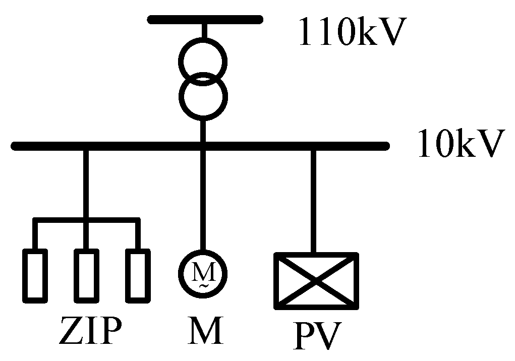
2. Generalized Load Model Structure

2.1. Traditional Load Model

The traditional load model mainly contains a static model, dynamic model, integrated load model, and non-mechanical models [16]. Initially, the ZIP model was used, and it consists of three parts: constant impedance, constant current, and constant power [17,18]. The Classical Load Model (CLM) proposed later is based on the ZIP model plus the induction motor model [16]. Later, the Synthesis Load Model (SLM) proposed by the China Electric Power Research Institute takes into account the equivalent impedance of the distribution network [19]. The structure of the three models is shown in the figure below (Figure 1).

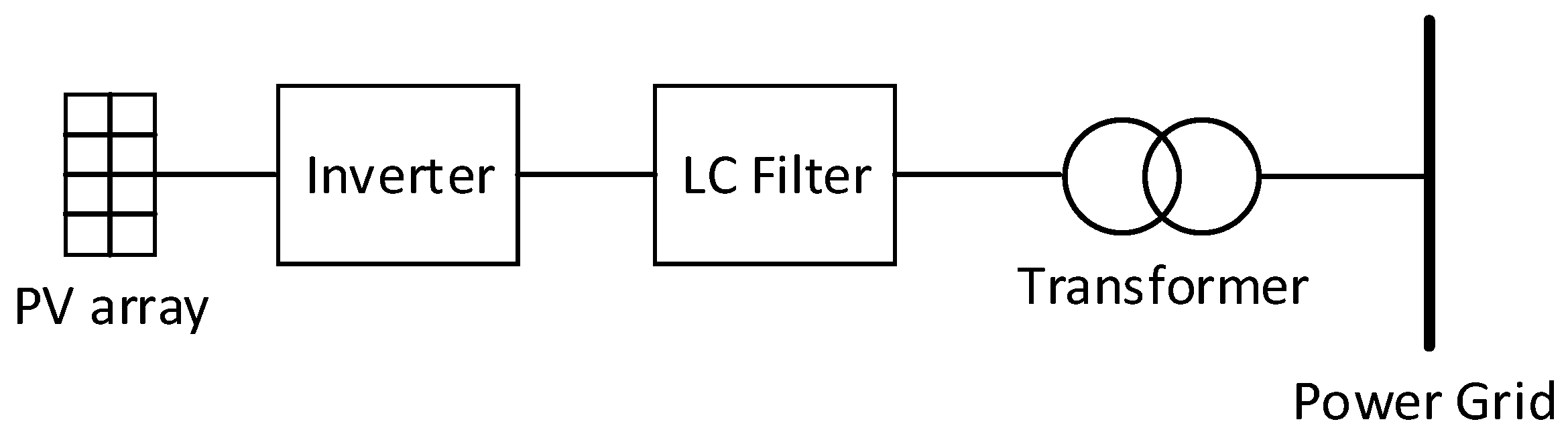
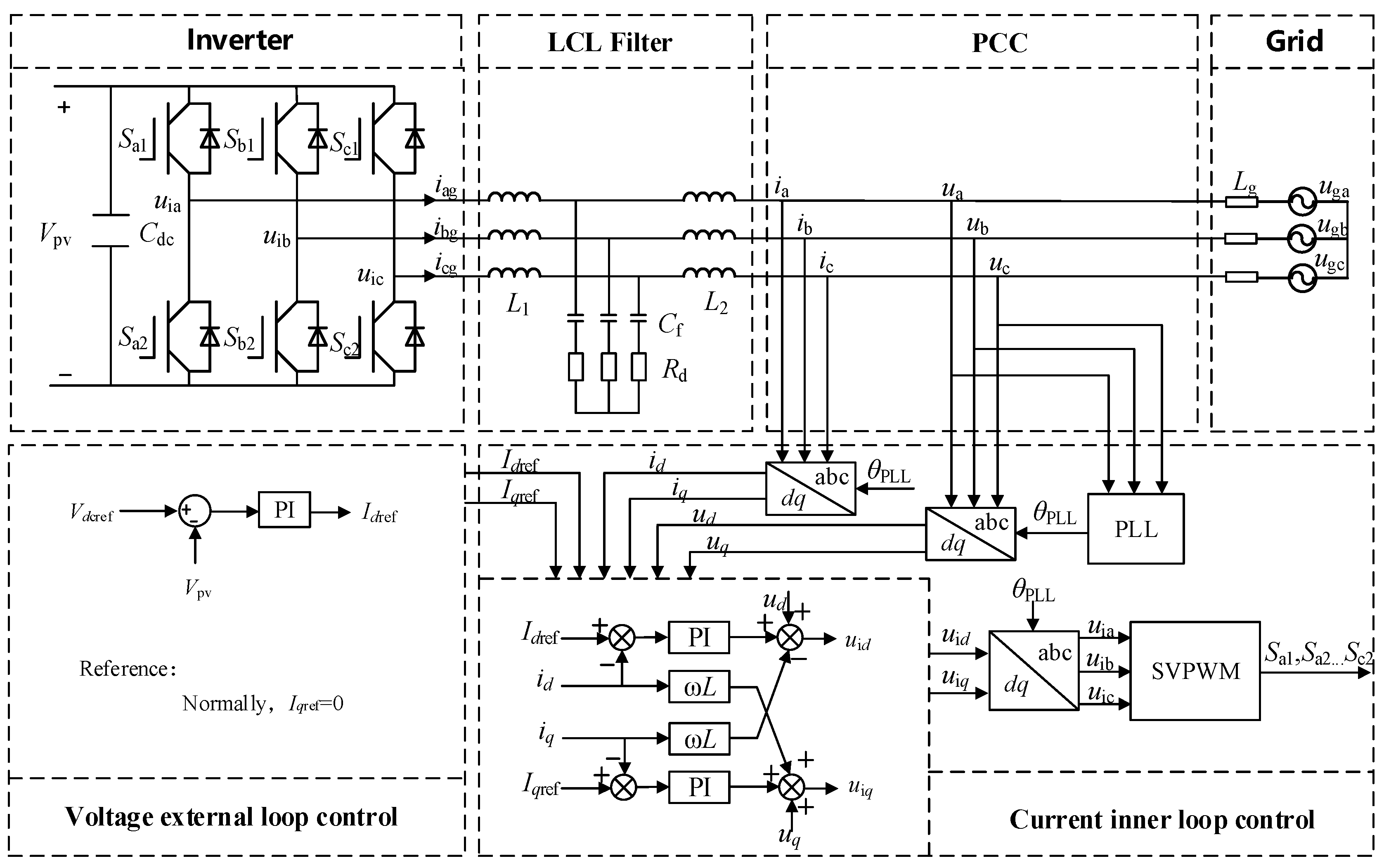
2.2. PV Power System Model and Grid-Connected Control

There are single-stage type and two-stage types of PV power generation systems, the former realizes the MPPT by a one-stage DC/AC session and connects the booster transformer [20,21]. As shown in the Figure 2. The photovoltaic effect converts solar energy into electrical energy, and the DC power collected by the panel is converted into AC power by the inverter, and then output by the filter and connected to the power grid.
When the PV system operates normally, the inverter follows a double closed-loop control strategy [22]. Figure 3 shows the structure of the grid-connected PV system and the overall control process of the inverter. Firstly, collecting the three-phase voltage and three-phase current at PCC. The three-phase cross-flow at the PCC is changed to a direct flow in the dq rotating coordinate system, while the whole PV grid system is controlled by controlling the direct flow. Then there is the voltage external loop control module, which obtains the grid current d-axis and q-axis component references Idref and Iqref through the PI control and negative feedback. The DC voltage reference is determined by the maximum power tracking link of the PV array link. However, the q-axis current reference in normal operation is generally taken as 0. The d-axis and q-axis reference values of the grid-connected currents output from the external loop are introduced into the inner-loop control link of the fixed active current id and reactive current iq current to obtain the d-axis component and q-axis component reference values of the voltage. Finally, the reference values of three-phase AC voltage are obtained based on the Park inverse transform. The control signals of the switching tubes in the three-phase bridge inverter circuit are generated by SVPWM control [23,24]. These steps realize a closed-loop control of the whole PV grid system.

2.3. Generalized Load Model

The generalized load model is obtained by improving on the CLM model. It connects the PV power system, static loads, and dynamic loads in parallel at the 10 kV virtual bus, which is boosted to 110 kV by a transformer and connected to the grid. The structure of the generalized load model is shown in Figure 4. The model enables dynamic modification of light intensity and temperature in PV systems and provides high and low voltage fault ride-through capability.
For the generalized load simulation model in this paper, a constant impedance load model is used for the static model and a third-order induction motor model is used for the dynamic load.

3. HVRT and LVRT of PV Inverters

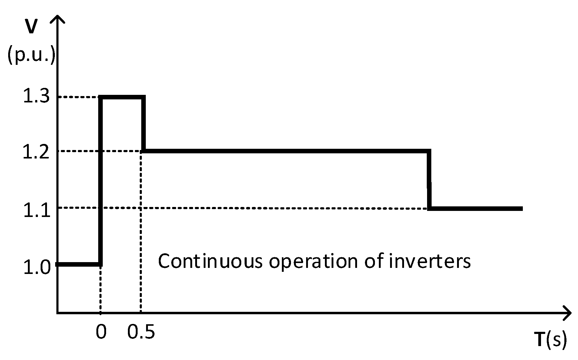
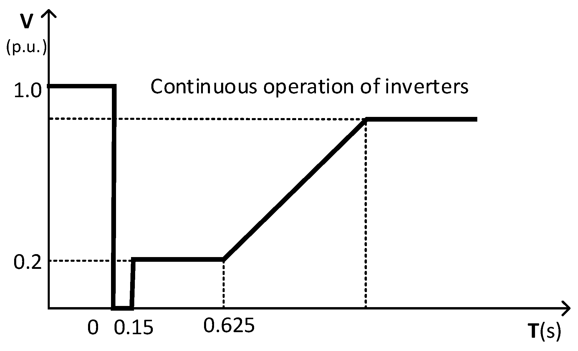
3.1. HVRT and LVRT Requirements of Distributed PV System

The Technology for Connecting Photovoltaic Power Plants to the Grid stipulates that PV power plants connected to the grid at voltage levels of 35 kV and above need to have high voltage and low voltage ride-through capability [25].
The specific requirements for high voltage ride-through in PV power plants are shown in Figure 5. The PV power plant is required to provide continuous active power regulation and the ability to inject reactive current into the grid during high voltage ride-through.
The specific requirements for low voltage ride-through in PV power plants are shown in Figure 6 [26]. It is required that the PV plants should be able to operate continuously without going off-grid for 0.15 s when the voltage at the grid-connected point of the PV plants drops to zero. The PV plants should also output reactive power to meet the voltage support of the system during voltage dips.

3.2. HVRT and LVRT Strategies of PV Inverters

The dynamic reactive power support capability of the inverter satisfies the following equations.
i q ref _ L = ( 0.9 U p ) × K , U p < 0.9 i q ref _ H = ( 1.1 U p ) × K , U p > 1.1
where K is the dynamic reactive power support factor. iqref_L and iqref_H are the reference values of reactive current under two kinds of faults, respectively.
The active and reactive current requirements of the inverter protection strategy during fault ride-through are shown in Figure 7. The inverter provides reactive power for both faults.

4. Parameters Identification and Simulation Verification for Generalized Load Model

4.1. Parameter Extraction for Generalized Load Models

In order to obtain the key parameters of the generalized load model and parameter identification benchmark data, a detailed electromagnetic transient model of the distribution network containing distributed PV is established based on PSCAD as shown in Figure 8. In this case, the generalized load model accesses the 110 kV bus.
In order to enable the model to fit different PV outputs and different load cases, the parameters shown in Table 1 are set as external given parameters.
The generalized load involves a total of 14 independent parameters that affect the power characteristics of each module, as shown in Table 2.
The proportion of static load active to total load active is kL = PL/(PL + PG), where PL is static load active power and PG is dynamic load active power.
Therefore, the sensitivity analysis method is utilized to determine the parameters having a greater influence on the model, only their parameters are identified, and the remaining parameters are selected as typical values to simplify the calculation volume [27].

4.2. Sensitivity Analysis of the Parameters

Under the given external parameter conditions of the distribution network in Figure 8, a parameter sensitivity analysis is performed to determine the key identification parameters under this power system.
As the dynamic reactive power support coefficients are involved, faults are set up at the parallel points of the detailed electromagnetic transient model. Then, the same small perturbation for each variable is set up to be recognized in turn. Finally, the active reactive power sensitivities of each variable are calculated.
The formula for calculating sensitivity is as follows.
S k ( t ) = lim Δ φ k 0 y φ 1 , , φ k   +   Δ φ k , , φ n , t     y φ 1 , , φ k , , φ n , t y φ 1 , , φ k , , φ n , t Δ φ k / φ k
where for the jth parameter φj to be identified at t, the output variable trace is yi with a variation of Δφj and a trace sensitivity of Sij. h is the number of parameters to be identified.
The steps are as follows,
  • Set up a three-phase symmetrical voltage dip fault at the parallel network point POC so that its duration is 0.5 s and the voltage dip amplitude is 20%, record the active power P0 and reactive power Q0 output from the parallel network point.
  • Increase the jth parameter by a factor of 0.1 and change the corresponding parameter in each element in the distribution network, set the same fault conditions as in the previous step, and record the active power Pj and reactive power Qj at the output of the grid point.
  • The active and reactive sensitivities are calculated separately through Equation (2). The average trajectory sensitivity is obtained by calculating the average of the two.
The sensitivity of each parameter calculated based on the above method is shown in Table 3 below.
The parameters in the table are arranged in order of average sensitivity from highest to lowest. Parameters with average sensitivities below 0.2 (RS, Xr, L, TE, KE, TI, KI) can be taken as fixed values, while parameters with sensitivities greater than 0.2 need to be re-identified to obtain results corresponding to specific operating conditions.

4.3. Identification of the Parameters

After determining the parameters to be identified, the next step is to identify these parameters. The steps for parameter identification are as follows.
  • On the one hand, the external input parameters of the generalized load model are determined according to the actual situation. On the other hand, determine the values of voltage, active, and reactive power at each node under normal operation and the occurrence of voltage dip faults at fixed locations through the detailed PSCAD model. These values are used as determinants to inform the parameter identification process.
  • The parameter identification follows the order of sensitivity from highest to lowest. Set the parameter to be recognized to an initial value and the rest to typical values.
  • A nonlinear least squares method based on the trust domain reflection algorithm is used to identify high-sensitivity parameters in a generalized load model. Calculating the sum of squares of the deviations of the operating results of the system containing the generalized load model from the test samples and using it as an objective function for optimization of the parameters to be identified.
  • Run the simulation with the identified results and compare the obtained results with the actual results, the identified parameter values can be accepted under the range of error operation, otherwise, re-identification is carried out.
Normal operation data and fault data of the grid are used as reference quantities for parameter identification. Voltage dip faults are set up at the 110 kV grid-connected points of the PV, and the voltage, active power, and reactive power data of each node before and after the fault are obtained. These data provide a reference for the identification process. Through multiple identifications, the average identification results or typical values for each parameter are obtained as shown in Table 4 below.
The last four parameters in the table are taken as typical values and are not involved in parameter identification due to their low sensitivity.

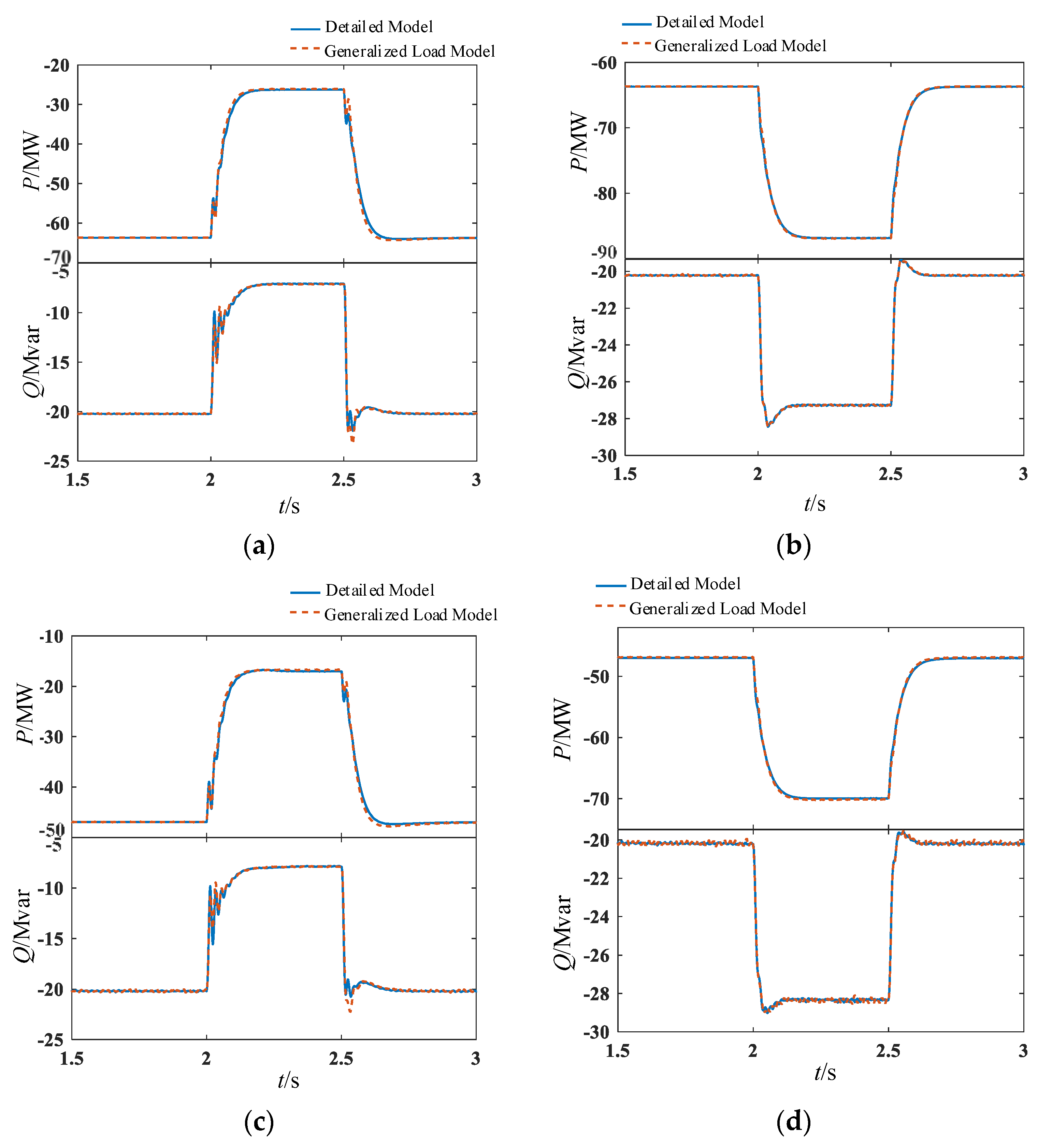
4.4. Simulation Validation of the Generalized Load Model

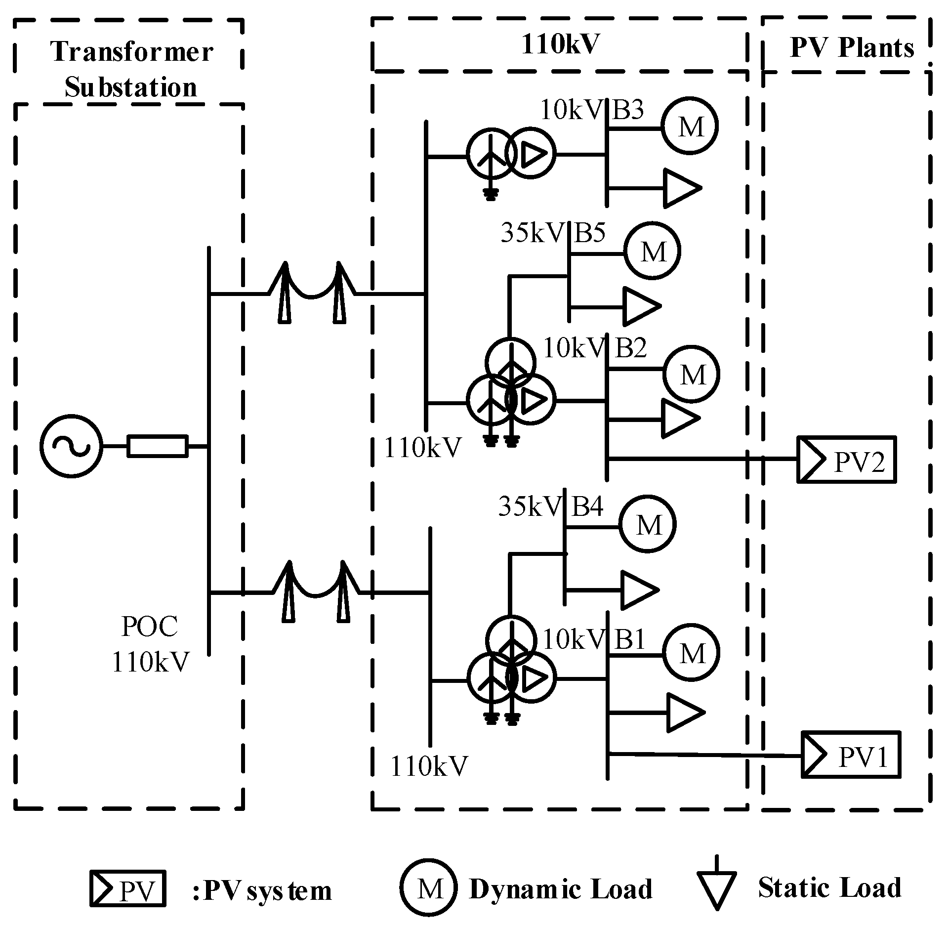
4.4.1. Detailed Distribution Network Model Calibration Based on Measured Data

Ideally, it is necessary to obtain the actual measured voltages and currents of the grid operation, which will be used as the test samples to demonstrate the validity of the identification model and parameters under the actual measured data. However, it is difficult to obtain the current data of the fault transient process in reality, so a detailed electromagnetic transient model of the distribution system with distributed photovoltaic access is adopted to test its ability to express the stable operation and fault transient characteristics of the actual distribution network.
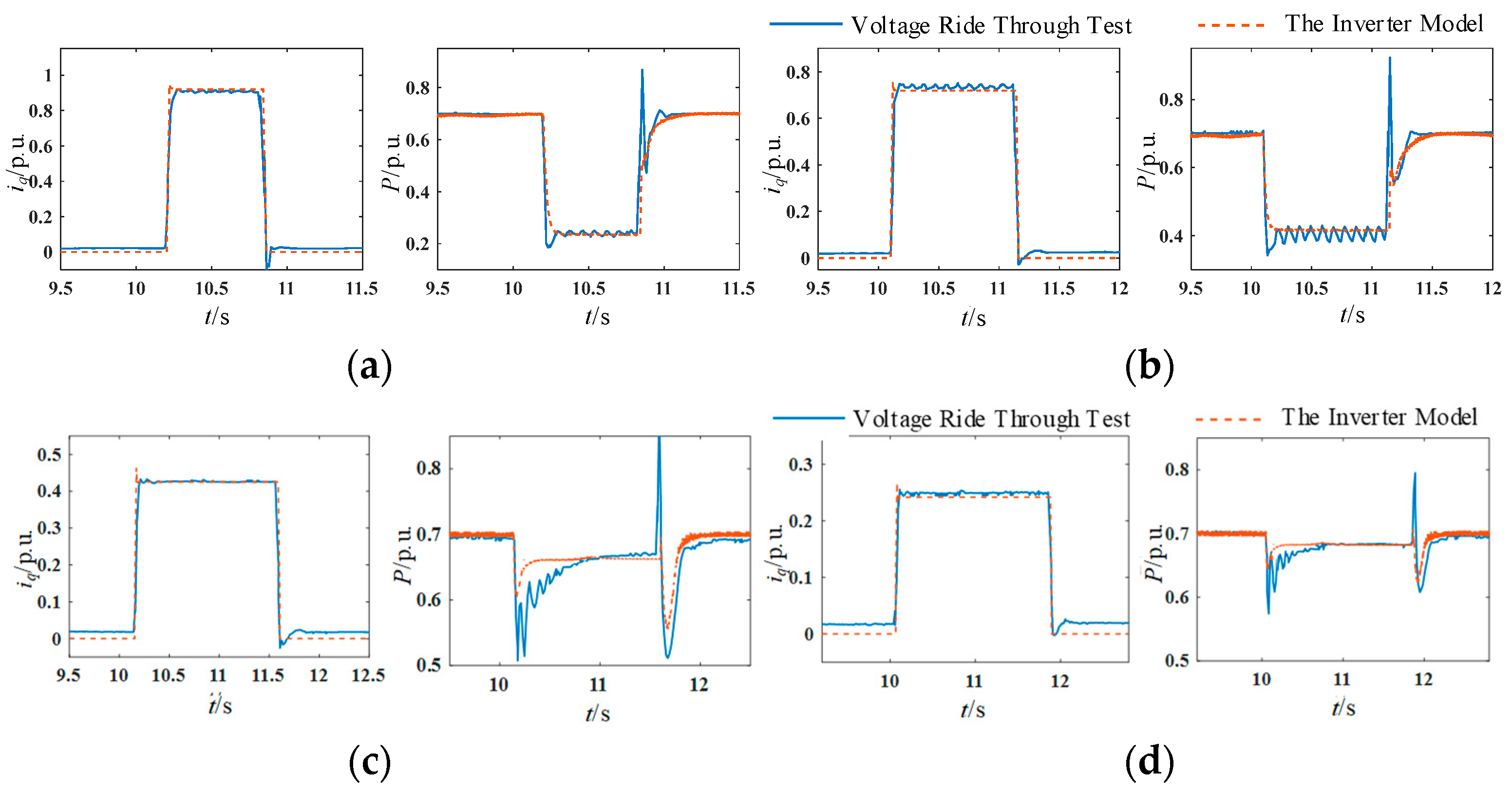
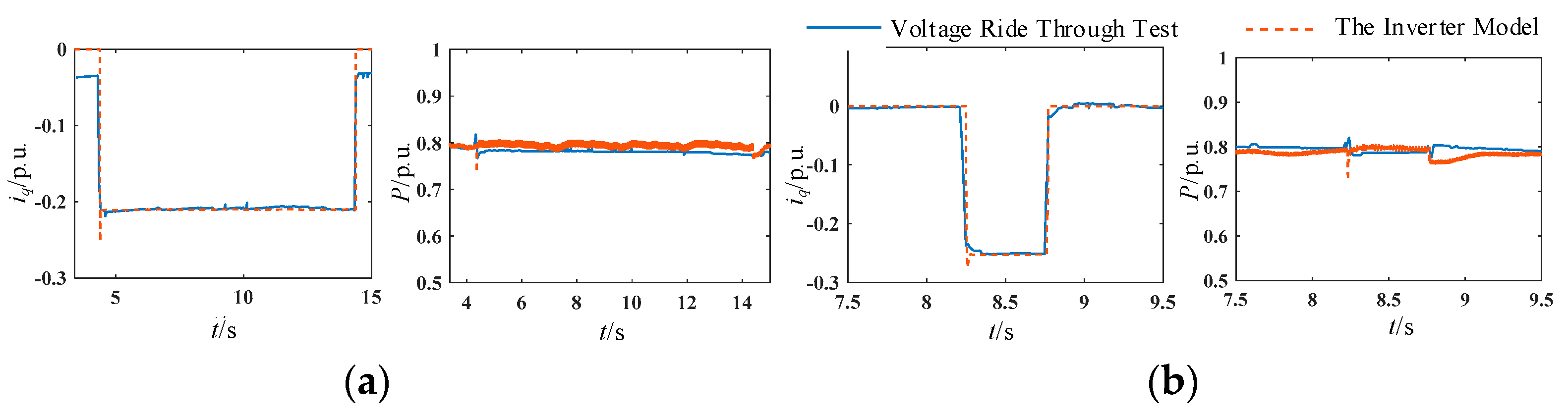
  • During the fault transient, the detailed electromagnetic transient model of the PV grid-connected inverter is calibrated based on the PV grid-connected inverter low-voltage and high-voltage ride-through test data to verify its accuracy.
  • During stable operation, based on the actual grid measurement data at a certain moment, combined with the light and temperature conditions at that moment, the PV grid-connected system detailed electromagnetic transient model of the PV output, and the steady state currents of each grid-connected point are calibrated.
  • With small errors, the detailed simulation model can reflect the operational state of the actual power grid. Subsequently, it can provide sufficient current data for the parameter identification of the generalized load model.
The inverter fault ride-through capability in the model is calibrated through simulation. The grid voltage drop amplitude is set to 80%, 60%, 40%, and 20% under 70% heavy load and symmetrical faults, respectively, and the LVRT faults form the grid voltage divider by casting the short circuit impedance. The reactive current and active output of the LVRT detection report and simulation model are shown in Figure 9. Under 80% heavy load and symmetrical faults, the amplitude of grid voltage rise is set to be 18% and 24%, respectively, and the high voltage ride-through fault raises the grid voltage by dropping the capacitor. The reactive current and active output of the high voltage ride-through detection report and simulation model are shown in Figure 10.
From Figure 9 and Figure 10, it can be seen that during the occurrence of a voltage dip fault, the active power P decreases and Id increases. At the occurrence of a voltage rise fault, the active output of the inverter is basically unchanged. During fault and fault recovery, the inverter reactive current and active dynamic response trends are basically consistent with the actual voltage ride-through detection report.
Under the stable operation state, based on the data obtained from the actual measurement of the distribution network at a certain moment, combined with the light and temperature conditions at that moment, the calibration of the PV output, 10 kV grid-connected points, and 110 kV grid-connected point currents in the detailed distribution network model is carried out.
The actual measurements of the power flow at a certain point in time were selected to calibrate the power flow at the five measurement points in Figure 8. The temperature at that moment is 33 °C, the light amplitude is 831.5 W/m2, and the distributed PV output is about 80% of the rated capacity. The actual measured data, simulation results, and relative error calculations at each point of the distribution network are shown in Table 5.
From the analysis of Table 5, it can be seen that the error between the actual PV output and the simulation results is below 2%, and the error between the measured steady-state current at the grid connection point and the simulation results is below 1%. It can be assumed that the electromagnetic transient model of the distribution network system with distributed PV access can reflect the actual grid operation state and the grid-connected data can be used as the benchmark data for the parameter identification of the generalized load model.

4.4.2. Generalized Load Model Calibration

The accuracy of the generalized load model is assessed by calculating the deviation between the detailed electromagnetic transient model of the distribution network and the generalized load model in PSCAD. The electrical quantities for the deviation calculation include grid point voltage Us, grid point current I, grid point active power P, and grid point reactive power Q. The deviation of the generalized load model from the detailed electromagnetic transient model in PSCAD is assessed by calculating the accuracy of the generalized load model.
The transient and steady-state deviations are calculated separately for each time period by dividing the region of the perturbation process. The region division is as follows (Figure 11).
  • Time period A starts 2 s before the voltage dip.
  • The first 20 ms of the voltage drop to 0.9 p.u. is the end of the A period and the beginning of the B period.
  • The first 20 ms of the start time of disturbance removal is the end of the B time period and the start of the C time period.
  • After the disturbance is cleared, 2 s after the system’s active power starts to stabilize its output is the end of the C time period.
The average deviation and maximum deviation are calculated as follows:
  • The average deviation in the steady state interval (F1) represents the arithmetic mean of the deviations between the detailed electromagnetic transient model and the generalized load model in the steady state interval.
F 1 = 1 K S _ E n d K S _ S t a r t + 1 i = K S _ S t a r t K S _ E n d X S i 1 K M _ E n d K M _ S t a r t + 1 i = K M _ S t a r t K M _ E n d X M i
where XS is the standardized value of the generalized load model simulation data of the electrical quantity to be assessed, XM is the standardized value of the detailed electromagnetic transient model simulation data of the electrical quantity to be assessed, KS_Start, KS_End are the first and the last serial numbers of the generalized load model simulation data within the calculation error interval, KM_Start, KM_End are the first and the last serial numbers of the detailed electromagnetic transient model simulation data within the calculation error interval.
  • The average deviation over the transient interval (F2) is the arithmetic mean of the deviations between the detailed electromagnetic transient model and the generalized load model over the transient interval.
F 2 = 1 K S _ E n d K S _ S t a r t + 1 i = K S _ S t a r t K S _ E n d X S i 1 K M _ E n d K M _ S t a r t + 1 i = K M _ S t a r t K M _ E n d X M i
  • The maximum deviation in the steady state interval (F3) is the maximum value of the deviation between the detailed electromagnetic transient model and the generalized load model in the steady state interval.
F 3 = max i = K M _ S t a r t K M _ E n d X S i X M i
The average deviation of each time period is calculated as a weighted average, and the weights of each time period are taken as follows: 10% for A (before the disturbance), 60% for B (during the disturbance), and 30% for C (after the disturbance).
In order to test the validity of the proposed generalized load model, based on the distribution system described above, tests are conducted under different PV penetration rates and voltage dips. Four sets of test samples are established as follows (Table 6). Different levels of fault falls are set at grid-connected points and different PV penetrations. The results of parameter identification are shown in Table 7. The deviation of the generalized load model is calculated as follows (Table 8).
The steady-state operation and fault transient characteristics of the generalized load model obtained by parameter identification for the above four samples are simulated, and the results are shown in Figure 12.
Table 7 shows the identification results of the high-sensitivity parameters corresponding to the four samples, and it can be seen that there is a small difference in the sensitivity identification results under different samples. Table 8 shows the results of bias calculations under each time interval for the four samples. Each deviation of the data in the table is less than 1%, which shows that the generalized load model has a better descriptive ability for the operation scenarios with different voltage dips and rises and different PV proportions of total loads. And Figure 12 verifies the above findings.

5. Conclusions

This paper focuses on proposing a generalized load model that considers the fault ride-through capability of distributed PV systems, summarized as follows.
  • A generalized load model that includes a detailed PV system structure and considers PV high and low voltage fault ride-through capability is developed. Compared with other load models, this model takes into account the PV high and low voltage ride-through characteristics, which are more adapted to the load characteristics of the real distribution network at present.
  • In the model calibration section, a detailed model calibration of the distribution network based on measured data is proposed. Considering that it is difficult to obtain the parameters of the actual grid fault, the detailed model based on measured data is first established to check its ability to express the stable operation and fault transient characteristics of the actual distribution network. From the simulation results, the error between the actual current and the detailed model is less than 1%, and it can be considered that the model can reflect the actual operation state of the grid. The grid-connected data can be used as the benchmark data for the parameter identification of the generalized load model.
  • After the parameter identification is completed, the generalized load model and the detailed model will be simulated. By comparing the simulation results under four groups of different PV penetration rates and different operating conditions, the errors of the corresponding physical quantities of the two models are calculated, and the resulting errors are less than 1%. The model fits well with the distributed PV access to the distribution network.

Author Contributions

Methodology, H.C.; Software, H.W. (Huayue Wei); Validation, H.W. (Huayue Wei); Investigation, H.W. (Haiyun Wang); Resources, Z.Z. and H.W. (Haiyun Wang); Data curation, Q.C.; Writing—original draft preparation, L.Z.; Writing—review and editing, X.Y.; Visualization, Z.Z.; Supervision, X.C. All authors have read and agreed to the published version of the manuscript.

Funding

This research was funded by State Grid Corporation of China, grant number 52022323000W. And The APC was funded by State Grid Corporation of China.

Data Availability Statement

The original contributions presented in the study are included in the article, further inquiries can be directed to the corresponding author.

Conflicts of Interest

Author Haiyun Wang, Qian Chen, Zhijian Zhang and Huayue Wei were employed by the company State Grid Beijing Electric Power Company Electric Power Scientific Research Institute. The remaining authors declare that the research was conducted in the absence of any commercial or financial relationships that could be construed as a potential conflict of interest.

References

  1. Karimi, M.; Mokhlis, H.; Naidu, K.; Uddin, S.; Bakar, A. Photovoltaic penetration issues and impacts in distribution network–A review. Renew. Sustain. Energy Rev. 2016, 53, 594–605. [Google Scholar] [CrossRef]
  2. Rahman, A.; Farrok, O.; Haque, M.M. Environmental impact of renewable energy source based electrical power plants: Solar, wind, hydroelectric, biomass, geothermal, tidal, ocean, and osmotic. Renew. Sustain. Energy Rev. 2022, 161, 112279. [Google Scholar] [CrossRef]
  3. Alsafasfeh, Q.; Saraereh, O.A.; Khan, I.; Kim, S. Solar PV grid power flow analysis. Sustainability 2019, 11, 1744. [Google Scholar] [CrossRef]
  4. Ding, M.; Wang, W.; Wang, X.; Song, Y.T.; Chen, D.Z.; Sun, M. A Review on the Effect of Large-scale PV Generation on Power Systems. Proc. CSEE 2014, 34, 1–14. [Google Scholar]
  5. Huang, W.; Dong, X.; Lei, J.; Yu, L. Integrated Impact of Large-capacity Distributed Photovoltaic on Power Grid. Proc. CSU-EPSA 2016, 28, 44–49. [Google Scholar]
  6. Zheng, W.; Xiong, X. A model identification method for photovoltaic grid-connected inverters based on the Wiener model. Proc. CSEE 2013, 33, 18–26. [Google Scholar]
  7. Liu, Z.; Wu, H.; Jin, W.; Xu, B.; Ji, Y.; Wu, M. Two-step method for identifying photovoltaic grid-connected inverter controller parameters based on the adaptive differential evolution algorithm. IET Gener. Transm. Distrib. 2017, 11, 4282–4290. [Google Scholar] [CrossRef]
  8. Paulescu, M.; Brabec, M.; Boata, R.; Badescu, V. Structured, physically inspired (gray box) models versus black box modeling for forecasting the output power of photovoltaic plants. Energy 2017, 121, 792–802. [Google Scholar] [CrossRef]
  9. Sun, G.; Zhang, J.; Wu, H. Research on the identification and adaptation of generalized load modeling based on distributed generators. Power Syst. Prot. Control 2013, 41, 105–111. [Google Scholar]
  10. Ma, Y.; Li, X.; Cao, J. Integrated load modeling with inverter-containing distributed power. J. Sol. Energy 2015, 36, 1869–1875. [Google Scholar]
  11. Samadi, A.; Soder, L.; Shayesteh, E.; Eriksson, R. Static equivalent of distribution grids with high penetration of PV systems. IEEE Trans. Smart Grid 2015, 6, 1763–1774. [Google Scholar] [CrossRef]
  12. Zhang, J.; Sun, Y. Impact of three-phase single-stage photovoltaic system on distribution network load modeling. Autom. Electr. Power Syst. 2011, 35, 73–78. [Google Scholar]
  13. Guan, L.; Zhao, Q.; Zhou, B.; Lyu, Y.; Zhao, W.; Yao, W. Multi-scale clustering analysis based modeling of photovoltaic power characteristics and its application in prediction. Autom. Electr. Power Syst. 2018, 42, 24–30. [Google Scholar]
  14. Qu, X.; Li, X.; Sheng, Y.; Su, Z.; Zhao, Y. Research on equivalent modeling of PV generation system for generalized load. Power Syst. Technol. 2020, 44, 2143–2150. [Google Scholar]
  15. Stetz, T.; Marten, F.; Braun, M. Improved low voltage grid-integration of photovoltaic systems in Germany. IEEE Trans. Sustain. Energy 2013, 4, 534–542. [Google Scholar] [CrossRef]
  16. Ju, P.; Ma, D. Power System Load Modeling, 2nd ed.; China Electric Power Press: Beijing, China, 2008; pp. 144–145. [Google Scholar]
  17. Zhang, R.; Chao, L.; Ying, W. A two-stage framework for ambient signal based load model parameter identification. Int. J. Electr. Power Energy Syst. 2020, 121, 106064. [Google Scholar] [CrossRef]
  18. Arif, A.; Wang, Z.; Wang, J.; Mather, B.; Bashualdo, H.; Zhao, D. Load modeling—A review. IEEE Trans. Smart Grid 2017, 9, 5986–5999. [Google Scholar] [CrossRef]
  19. China Electric Power Research Institute. Power System Analysis Synthesis Program Version 6. 0 User Manual; China Electric Power Research Institute: Beijing, China, 2000; pp. 1–200. [Google Scholar]
  20. Kabir, M.N.; Mishra, Y.; Ledwich, G.; Dong, Z.Y.; Wong, K.P. Coordinated control of grid-connected photovoltaic reactive power and battery energy storage systems to improve the voltage profile of a residential distribution feeder. IEEE Trans. Ind. Inform. 2014, 10, 967–977. [Google Scholar] [CrossRef]
  21. Kumary, S.V.S.; Oo, V.A.A.M.T.; Shafiullah, G.M.; Stojcevski, A. Modelling and power quality analysis of a grid-connected solar PV system. In Proceedings of the 2014 Australasian Universities Power Engineering Conference (AUPEC), Perth, Australia, 28 September–1 October 2014; pp. 1–6. [Google Scholar]
  22. Jin, X.; Wen, S.; Ni, H.; Yang, Y.; Wen, Y. Review of maximum power point tracking of photovoltaic system. Chin. J. Power Sources 2019, 43, 532–535. [Google Scholar]
  23. Rajlaxmi, E.; Behera, S.; Panda, S.K. Comparison of Inverter Control by SPWM and SVPWM Method in Standalone PV System. In Proceedings of the 2020 IEEE International Symposium on Sustainable Energy, Signal Processing and Cyber Security (iSSSC), Gunupur Odisha, India, 16–17 December 2020. [Google Scholar]
  24. Hassaine, L.; Olias, E.; Quintero, J.; Salas, V. Overview of power inverter topologies and control structures for grid connected photovoltaic systems. Renew. Sustain. Energy Rev. 2014, 30, 796–807. [Google Scholar] [CrossRef]
  25. Li, F.; Liu, M.; Wang, Y.; Zhang, X. Research on HIL-based HVRT and LVRT automated test system for photovoltaic inverters. Energy Rep. 2021, 7, 405–412. [Google Scholar] [CrossRef]
  26. Al-Shetwi Ali, Q.; Sujod, M.Z.; Blaabjerg, F. Low voltage ride-through capability control for single-stage inverter-based grid-connected photovoltaic power plant. Sol. Energy 2018, 159, 665–681. [Google Scholar] [CrossRef]
  27. Guo, L.; Meng, Z.; Sun, Y.; Wang, L. Parameter identification and sensitivity analysis of solar cell models with cat swarm optimization algorithm. Energy Convers. Manag. 2016, 108, 520–528. [Google Scholar] [CrossRef]
Figure 1. Structure of the Traditional Load Model. (a) ZIP model (b) CLM model (c) SLM model.
Energies 17 03595 g001
Figure 2. Structure of Single-Stage Type.
Energies 17 03595 g002
Figure 3. Structure of the grid-connected PV system and the overall control process of the inverter.
Energies 17 03595 g003
Figure 4. Structure of generalized load model.
Energies 17 03595 g004
Figure 5. High voltage ride-through requirement.
Energies 17 03595 g005
Figure 6. Low voltage ride-through requirement.
Energies 17 03595 g006
Figure 7. Diagram of inverter protection control strategy.
Energies 17 03595 g007
Figure 8. Structure of the distribution network with distributed PV plants.
Energies 17 03595 g008
Figure 9. Low voltage ride-through validation of PV inverter: (a) 80% voltage drop, (b) 60% voltage drop, (c) 40% voltage drop, (d) 20% voltage drop.
Energies 17 03595 g009
Figure 10. High voltage ride-through validation of PV inverter: (a) 18% voltage increase, (b) 24% voltage increase.
Energies 17 03595 g010
Figure 11. Division of time periods.
Energies 17 03595 g011
Figure 12. Curves for simulation. (a) Sample 1. (b) Sample 2. (c) Sample 3. (d) Sample 4.
Energies 17 03595 g012
Table 1. The external parameters.
NO.ParameterNotation
1Active Power of Static Loads and Dynamic LoadsP
2Number of PV unitsnPV
3Intensity of lightS
4Celsius temperatureT
Table 2. Parameters within the module.
NO.ParameterNotation
1Ration of Active Power for Static LoadskL
2Power Factor of ZIP Loadsθ
3Stator Resistance for Dynamic LoadsRS
4Stator Reactance for Dynamic LoadsXS
5Rotor Resistance for Dynamic LoadsRr
6Rotor Reactance for Dynamic LoadsXr
7Excitation Reactance for Dynamic LoadsXm
8Rated turndown for Dynamic LoadssN
9Inductance at Inverter ExitL
10Proportional Coefficient of External SegmentKE
11Integral Time Constant of External SegmentTE
12Proportional Coefficient of Internal SegmentKI
13Integral Time Constant of Internal SegmentTI
14Dynamic Reactive Power Support FactorK
Table 3. Conventional load parameters.
ParameterActive PowerReactive PowerAverages
K0.00906.89723.4531
θ0.10544.36582.2356
sN0.29953.81112.0553
Rr0.26243.12561.6940
kL1.75630.51221.1343
Xm0.03361.93560.9846
XS0.05510.21290.6340
RS0.01190.38640.1992
Xr0.00560.30390.1547
L0.02410.23840.1312
TE0.04070.10660.0736
KE0.03090.10350.0672
TI0.00150.08730.0444
KI0.00150.06270.0321
Table 4. Parameters identification results.
NO.ParameterAverages
1K1.5742
2KL0.8432
3θ0.9776
4sN0.9634
5Rr0.0301
6Xm2.4124
7XS0.1677
8RS0.0282
9Xr0.0253
10L0.0994
11TE0.0980
12KE3
13TI0.012
14KI0.2
Table 5. Measurement data, simulation data, and errors.
PointMeasurement DataSimulation DataRelative Error
P/MWQ/MVarP/MWQ/MVarP/MWQ/MVar
16.786.711.03
22.452.491.63
32.242.152.252.160.4460.465
44.6604.670.0050.2140.497
59.532.049.562.040.3140
Table 6. Data for samples.
SampleConditionsPV Penetration
1Voltage dropped by 20%0.15
2Voltage increased by 15%0.15
3Voltage dropped by 20%0.30
4Voltage increased by 15%0.30
Table 7. Results of parameter identification.
SampleKLθRr/p.u.Xm/p.u.SNK
10.77610.98100.03452.53790.95981.6248
20.79420.97930.02672.54560.96901.1186
30.81440.98010.02782.72800.96751.3866
40.80680.98040.02612.76860.96970.9650
Table 8. The deviation of the generalized load model.
F1/F2F3Weighted Deviations
UIPQUIPQUIPQ
Sample1A0.00020.00010.00010.00020.00130.00030.00060.00110.00030.00120.00190.0004
B10.00070.00410.00390.0003
B20.00020.00060.00160.00070.00100.00090.00210.0012
C10.00040.00670.00970.00001
C20.00020.00010.00010.00020.00130.00040.00150.0011
Sample2A0.00030.00010.00040.00010.00130.00050.00080.001150.00150.00060.00060.0002
B10.00100.00390.00010.0002
B20.00030.00010.00060.000090.00150.00040.00120.0015
C10.00220.00210.00080.0002
C20.00030.00020.00070.00010.00130.00060.00120.0011
Sample3A0.00010.000060.00030.00040.00130.00090.00150.00360.00240.00190.00240.0004
B10.00350.00900.00660.0005
B20.00010.00110.00320.00040.00100.00210.00460.0022
C10.00520.00480.00030.0010
C20.00010.00010.00020.00020.00130.00100.00230.0032
Sample4A0.00010.00060.00170.00050.00130.00150.00310.00380.00260.00130.00210.0003
B10.00380.00520.00220.0003
B20.00020.00040.00190.00010.00160.00120.00370.0041
C10.00200.00280.00170.0002
C20.00010.00100.00270.00060.00140.00190.00430.0038
Disclaimer/Publisher’s Note: The statements, opinions and data contained in all publications are solely those of the individual author(s) and contributor(s) and not of MDPI and/or the editor(s). MDPI and/or the editor(s) disclaim responsibility for any injury to people or property resulting from any ideas, methods, instructions or products referred to in the content.

