The Behavior of Terminal Voltage and Frequency of Wind-Driven Single-Phase Induction Generators under Variations in Excitation Capacitances for Different Operating Conditions

Abstract

This paper assesses the behavior of output voltage and frequency of wind-driven self-excited induction generators with variable excitation capacitances connected to the main and auxiliary windings under different operating conditions. The optimum values of the main winding excitation capacitance for fixed terminal voltage operation under different values of shunt capacitance, load, and speed are also evaluated. The obtained results show that the terminal voltage is highly affected by changing the main winding excitation capacitance. In addition, the frequency is greatly affected by changing the auxiliary winding excitation capacitance. However, under different operating conditions, variation in the output frequency under different values of the main winding capacitance, with fixed auxiliary winding capacitance, is acceptable. Extensive simulations were conducted and the results are discussed in this publication.

1. Introduction

Currently, electric energy demand is rising rapidly combined with certain environmental regulations for gas emissions in some countries [1,2]. On the other hand, around twenty-five percent of the world’s inhabitants living in remote areas are not fed by the main electric grids. Moreover, many residents in developing countries obtain their energy needs from conventional biomass, which negatively affects their health [3]. These factors, combined with the inherent merits of renewable energy resources, are rapidly replacing conventional energy sources, such as fossil fuel, with renewable resources including wind, solar, hydropower, biomass, and earth heat [4,5]. Wind energy is one of the most attractive and promising choices for generating electricity in remote areas due to noticeable growth in the small wind turbine industry [6].

Most standalone wind energy/electricity conversion systems implement squirrel cage induction generators due to their advantages over synchronous or DC generators. They also require less maintenance since they have no brushes or commutators in the absence of a DC excitation source and ruggedness [7,8,9,10,11]. Single-phase self-excited induction generators (SPSEIGs) are the preferable choice for stand-alone small power generation to serve as an emergency power source or main source to feed low-scale power loads in rural and remote areas [12,13,14,15]. A two-capacitor single-phase induction motor can be used as a self-excited induction generator by providing the appropriate excitation capacitors to its two windings and driving it at a suitable speed. When SPSEIG is run at an appropriate speed, the residual flux in the generator cores, combined with excitation capacitors, initiates voltage buildup. The process of self-excitation continues until the rated terminal voltage is attained at saturation [16].

The main disadvantage of implementing a wind-driven single-phase self-excited induction generator is the variation in the output terminal voltage and frequency under variations in wind speed or supplied load. Publications that address this problem are limited; therefore, extensive research work must be conducted to enhance the literature in this area. Sabha Raj Arya et al. [17] implemented a voltage source converter across the main winding to regulate the terminal voltage and frequency of SPSEIG under different conditions. They used a control approach based on adaptive theory to improve power quality. In [18], SPSEIG output voltage and frequency were regulated by fixing the generator’s output power to a controlled dump load connected to the main winding and consumer load. They used a DSP to control the switching of a PWM AC chopper, which was connected to a dump load. Mossad et al. [19] regulated the terminal voltage of a wind-driven single induction generator by adjusting the effective capacitance value of the capacitor connected across the auxiliary winding using a PI controller with an optimized algorithm. A simple control approach to adjusting the output voltage of SPSEIG was achieved by Ahshan and Iqba [20], who implemented a PI controller to control the dump load through an analog input power controller (AIPC). Olorunfemi Ojo et al. [21] used a single-phase bridge inverter fed by a battery to control the voltage and frequency of a two-capacitor SPSEIG. Depending on the real power generated, a battery can feed the generator or be recharged. The required reactive power is provided by the capacitor across the load and inverter.

The main contribution of the current publication is the behavioral assessment of the terminal voltage and output frequency of wind-driven stand-alone SPSEIG in response to changes in excitation capacitances connected to the auxiliary and main windings under different operating conditions. The other important contribution is the estimation of optimum excitation capacitances to achieve fixed terminal voltage under different loads and speed conditions with acceptable variation in the output frequency.

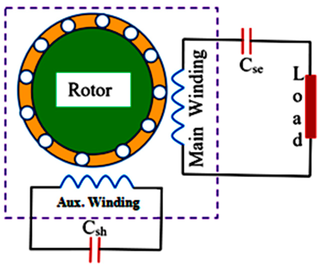
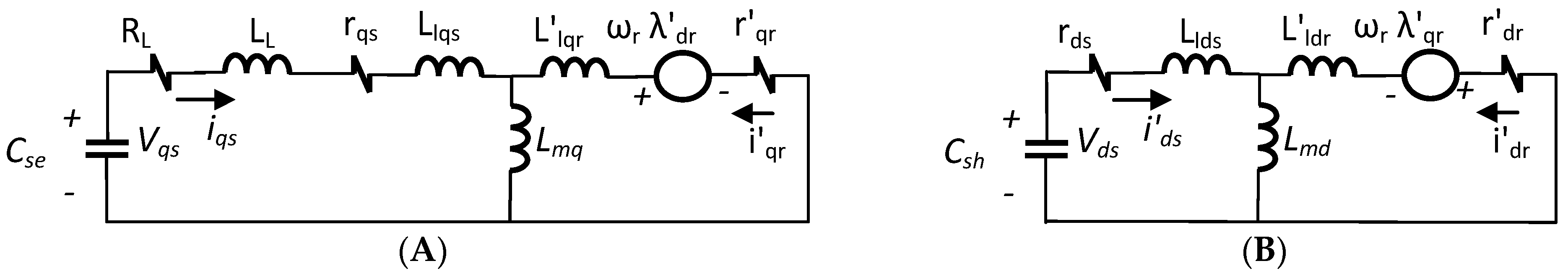
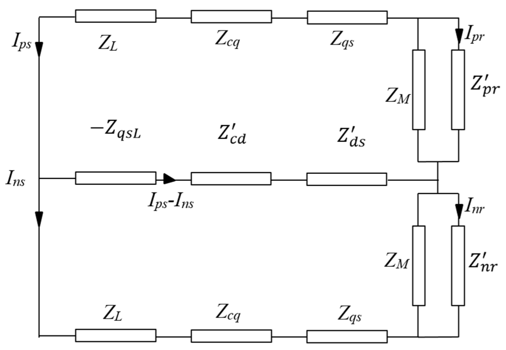
2. Modeling of Single-Phase Self-Excited Induction Generator

Figure 1 shows a schematic diagram of the single-phase self-excited induction generator considered in the current research work. A C_sh capacitor is connected across the auxiliary winding and a C_se capacitor is connected in series to the main winding and supplied load.

Based on the schematic diagram of the SPSEIG system shown in Figure 1 [22,23], the q-axis and d-axis equivalent circuits of SPSEIG in the stationary reference frame are presented in Figure 2A,B. Using the qd-equivalent circuits, the dynamic model of the generator in a stationary reference frame is presented in Equations (1)–(4), which derive dynamic equations to conduct simulations for SPSEIG, as presented in Appendix A. The generator’s steady-state model can be derived by replacing the derivative operator and integrator of the dq dynamic model with $j{\omega }_e$ and ${\displaystyle \frac{1}{j{\omega }_e}}$, respectively [9,22]. The resulting two matrix equations are provided in Equations (5) and (6).

$$v_{qs}=\left(r_{qs}+R_L\right)i_{qs}+{\displaystyle \frac{d}{dt}}{(\lambda }_{qs}+{\lambda }_{L_L})=-{\displaystyle \frac{1}{C_{se}}}\int i_{qs}dt$$

(1)

$$v_{ds}^{\prime }=r_{ds}^{\prime }{i}_{ds}^{\prime }+{\displaystyle \frac{d{\lambda }_{ds}}{dt}}=-{\displaystyle \frac{1}{C_{sh}}}\int i_{ds}^{\prime }dt$$

(2)

$$v_{qr}^{\prime }=r_r^{\prime } i_{qr}^{\prime }-{\lambda }_{dr}{\displaystyle \frac{d {\theta }_r}{dt}}+{\displaystyle \frac{d {\lambda }_{qr}}{dt}}$$

(3)

$$v_{dr}^{\prime }=r_r^{\prime } i_{dr}^{\prime }+{\lambda }_{qr}{\displaystyle \frac{d {\theta }_r}{dt}}+{\displaystyle \frac{d {\lambda }_{dr}}{dt}}$$

(4)

$$\begin{array}{l}\left[\begin{array}{c}{v}_{qs}^s\\ v_{ds}^{s^{\prime }}\end{array}\right]=\left[\begin{array}{cc}{(r}_{qs}+R_L)+{j{\omega }_e(L}_s+L_L)& 0\\ 0& r_{ds}^{\prime }+j{\omega }_e{L}_s\end{array}\right]\left[\begin{array}{c}{i}_{qs}^s\\ i_{ds}^{s^{\prime }}\end{array}\right]+\left[\begin{array}{cc}{j{\omega }_{e}L}_m& 0\\ 0& j{\omega }_e{L}_m\end{array}\right]\left[\begin{array}{c}\acute{i_{qr}^s}\\ \acute{i_{dr}^s}\end{array}\right]\\ ={\displaystyle \frac{1}{j{\omega }_e}}\left[\begin{array}{c}-{\displaystyle \frac{1}{C_{se}}} 0\\ 0-{\displaystyle \frac{1}{C_{sh}}}\end{array}\right]\left[\begin{array}{c}{i}_{qs}^s\\ i_{ds}^{s\prime }\end{array}\right]\end{array}$$

(5)

$$\left[\begin{array}{c}{v}_{qr}^{s\prime }\\ v_{dr}^{s\prime }\end{array}\right]=\left[\begin{array}{cc}{\acute{r_r}+j\omega }_e{L}_r& {-\omega }_r{L}_r\\ {\omega }_r{L}_r& \acute{r_r}+{j\omega }_e{L}_r\end{array}\right]\left[\begin{array}{c}\acute{i_{qr}^s}\\ \acute{i_{dr}^s}\end{array}\right]+\left[\begin{array}{cc}{{j\omega }_{e}L}_m& -{{\omega }_{r}L}_m\\ {{\omega }_{r}L}_m& {{j\omega }_{e}L}_m\end{array}\right]\left[\begin{array}{c}{i}_{qs}^s\\ i_{ds}^s\end{array}\right]$$

(6)

Based on the relationship between the rms time phasors of the positive and negative sequence components, as well as the rms time phasor of the components on the qd-axis, it is possible to obtain the following positive and negative sequences of stator voltages with the help of the derivation procedure presented in [22]:

$$\begin{array}{l}{V}_{ps}={(r}_{qs}+R_L)I_{ps}+\left({\displaystyle \frac{r_{ds}^{\prime }-{(r}_{qs}+R_L)}{2}}\right)\left(I_{ps}-I_{ns}\right)+{j{\omega }_e(L}_{lqs}+L_L)I_{ps}+\\ {\displaystyle \frac{j{\omega }_e{L}_{lds}^{\prime }-{j{\omega }_e(L}_{lqs}+L_L)}{2}}\left(I_{ps}-I_{ns}\right)+{j{\omega }_{e}L}_M({I_{ps}+I}_{pr})\end{array}$$

(7)

$$\begin{array}{l}{V}_{ns}={(r}_{qs}+R_L)I_{ns}+{\displaystyle \frac{r_{ds}^{\prime }-{(r}_{qs}+R_L)}{2}}\left(I_{ns}{-I}_{ps}\right)+{j{\omega }_e(L}_{lqs}+L_L)I_{ns}+\\ {\displaystyle \frac{j{\omega }_e{L}_{lds}^{\prime }-{j{\omega }_e(L}_{lqs}+L_L)}{2}}\left(I_{ns}{-I}_{ps}\right)+{j{\omega }_{e}L}_M{(I}_{ns}+I_{nr})\end{array}$$

(8)

The qdsteady-state of stator voltages can be expressed in terms of excitation capacitors, as shown in the Equation (9) matrix. This equation can be transformed into positive and negative sequence components, as shown in Equations (10) and (11).

$$\left[\begin{array}{c}{V}_{qs}^s\\ V_{ds}^{s\prime }\end{array}\right]={\displaystyle \frac{1}{j{\omega }_e}}\left[\begin{array}{cc}-{\displaystyle \frac{1}{C_{se}}}& 0\\ 0& -{\displaystyle \frac{1}{C_{sh}}}\end{array}\right]\left[\begin{array}{c}{i}_{qs}^s\\ i_{ds}^{s\prime }\end{array}\right]$$

(9)

$$V_{ps}=j{\displaystyle \frac{1}{{{\omega }_{e}C}_{se}}}{I}_{ps}+{\displaystyle \frac{1}{2}}j({\displaystyle \frac{1}{{{\omega }_{e}C}_{sh}}}-{\displaystyle \frac{1}{{{\omega }_{e}C}_{se}}})(I_{ps}-I_{ns})$$

(10)

$$V_{ns}=j{\displaystyle \frac{1}{{{\omega }_{e}C}_{se}}}{I}_{ns}+{\displaystyle \frac{1}{2}}j({\displaystyle \frac{1}{{{\omega }_{e}C}_{sh}}}-{\displaystyle \frac{1}{{{\omega }_{e}C}_{se}}})(I_{ns}-I_{ps})$$

(11)

Equations (7) and (10) are combined in Equation (12) since they are equivalent. Moreover, Equations (8) and (11) are combined in Equation (13) for the same reason. The transformed equations of positive and negative components for the rotor side can be obtained by following the same procedure and considering the reality of zero rotor voltages, along with the slip equation: $s={\displaystyle \frac{{\omega }_e-{\omega }_r}{{\omega }_e}}$, as shown in the Equation (14) matrix. Based on Equations (12)–(14), the equivalent circuit of the positive and negative sequence components for SPSEIG feeding RL-Load at the rated frequency is presented in Figure 3. All the parameters in this circuit are defined in terms of per-unit frequency (the ratio of the operating frequency to the rated frequency); $F={\displaystyle \frac{\acute{f}}{f_b}}={\displaystyle \frac{\acute{{\omega }_e}}{{\omega }_b}}$. In addition, all impedances, except for the magnetizing impedance, were assumed to be fixed and independent of the operating frequency.

$$\begin{array}{l}0={(r}_{qs}+R_L)I_{ps}+\left({\displaystyle \frac{r_{ds}^{\prime }-{(r}_{qs}+R_L)}{2}}\right)\left(I_{ps}-I_{ns}\right)+{j{\omega }_e(L}_{lqs}+L_L)I_{ps}+{\displaystyle \frac{j{\omega }_e{L}_{lds}^{\prime }-{j{\omega }_e(L}_{lqs}+L_L)}{2}}\left(I_{ps}-I_{ns}\right)+\\ { j{\omega }_{e}L}_M\left({I_{ps}+I}_{pr}\right)-j{\displaystyle \frac{1}{{{\omega }_{e}C}_{se}}}{I}_{ps}-{\displaystyle \frac{1}{2}}j({\displaystyle \frac{1}{{{\omega }_{e}C}_{sh}}}-{\displaystyle \frac{1}{{{\omega }_{e}C}_{se}}})(I_{ps}-I_{ns})\end{array}$$

(12)

$$\begin{array}{l}0={(r}_{qs}+R_L)I_{ns}+{\displaystyle \frac{r_{ds}^{\prime }-{(r}_{qs}+R_L)}{2}}\left(I_{ns}{-I}_{ps}\right)+{j{\omega }_e(L}_{lqs}+L_L)I_{ns}+{\displaystyle \frac{j{\omega }_e{L}_{lds}^{\prime }-{j{\omega }_e(L}_{lqs}+L_L)}{2}}+{j{\omega }_{e}L}_M{(I}_{ns}+I_{nr})-\\ j{\displaystyle \frac{1}{{{\omega }_{e}C}_{se}}}{I}_{ns}-{\displaystyle \frac{1}{2}}j({\displaystyle \frac{1}{{{\omega }_{e}C}_{sh}}}-{\displaystyle \frac{1}{{{\omega }_{e}C}_{se}}})(I_{ns}-I_{ps})\end{array}$$

(13)

$$\left[\begin{array}{c}0\\ 0\end{array}\right]=\left[\begin{array}{cc}{\displaystyle \frac{\acute{r_r}}{s}}+j{\omega }_e\acute{L_{lr}}& 0\\ 0& {\displaystyle \frac{\acute{r_r}}{2-s}}+j{\omega }_e\acute{L_{lr}}\end{array}\right]\left[\begin{array}{c}{I}_{pr}\\ I_{nr}\end{array}\right]+\left[\begin{array}{cc}{j\omega }_e{L}_M& 0\\ 0& j{\omega }_e{L}_M\end{array}\right]\left[\begin{array}{c}{I}_{ps}+I_{pr}\\ I_{ns}+I_{nr}\end{array}\right]$$

(14)

The impedances in the circuit of Figure 3 are defined as follows:

$$\begin{array}{l}{Z}_{qs}={\displaystyle \frac{r_{qs}}{F}}+{j{\omega }_{b}L}_{lqs}\hspace{1em}{Z}_{cq}=-j{\displaystyle \frac{1}{F^2}}({\displaystyle \frac{1}{{{\omega }_{e}C}_{se}}})\hspace{1em}\hspace{1em}{Z}_L={\displaystyle \frac{R_L}{F}}+{j{\omega }_{b}L}_L\\ Z_{pns}={\displaystyle \frac{1}{2}}{[(Z}_{ds}^{\prime }+Z_{cd}^{\prime })-Z_{qsL}]\\ Z_{ds}^{\prime }={\displaystyle \frac{1}{a^2}}{\displaystyle \frac{r_{ds}}{F}}+{j{\omega }_{b}L}_{lds})\hspace{1em}\hspace{1em}{Z}_{cd}^{\prime }=-j{\displaystyle \frac{1}{F^2}}({\displaystyle \frac{1}{a^2}})({\displaystyle \frac{1}{{{\omega }_{b}C}_{sh}}})\hspace{1em}{Z}_{qsL}=Z_{qs}+Z_{cq}\\ Z_{pr}^{\prime }={\displaystyle \frac{\acute{r_r}}{F-n}}+j{\omega }_b\acute{L_{lr}}={\displaystyle \frac{1}{a^2}}({\displaystyle \frac{r_r}{F-n}}+j{\omega }_b{L}_{lr})\\ Z_{nr}^{\prime }={\displaystyle \frac{\acute{r_r}}{F+n}}+j{\omega }_b\acute{L_{lr}}={\displaystyle \frac{1}{a^2}}({\displaystyle \frac{r_r}{F+n}}+j{\omega }_b{L}_{lr})\hspace{1em}\hspace{1em}\hspace{1em}{Z}_M=j{\omega }_b{L}_m\end{array}$$

The total impedance equation of the circuit in Figure 3 is expressed by Equation (15). This non-linear equation has six unknowns: operating frequency F, speed n, magnetizing reactance X_M, load impedance Z_L, series capacitance C_se, and shunt capacitance C_sh. Therefore, a numerical solution should be applied to determine these required unknowns. Once these unknowns are determined, the generator’s steady-state performance, including the terminal voltage, can be evaluated.

$$Z_T=[({\displaystyle \frac{Z_M{Z}_{nr}^{\prime }}{Z_M+Z_{nr}^{\prime }}}+Z_{qsL})//Z_{pns}]+Z_{qsl}+{\displaystyle \frac{Z_M{Z}_{pr}^{\prime }}{Z_M+Z_{pr}^{\prime }}}$$

(15)

3. Results and Discussion

Figure 4 shows the terminal voltage (V_T) behavior with series excitation capacitance (C_se) for different values of shunt excitation capacitance (C_sh) at rated load and rated speed (Z_L = 1 pu, n = 1 pu). The terminal voltage increases in a non-linear manner by increasing the series excitation capacitance for fixed shunt excitation capacitance. On the other hand, the terminal voltage decreases by increasing the shunt excitation capacitance for the same series excitation capacitance values. For example, when C_se is 50 μF, V_T values corresponding to C_sh values of 30 μF, 60 μF, 75 μF, and 90 μF are 0.6654, 0.603, 0.5569, and 0.473 pu, respectively.

The output frequency (F) behavior against series excitation capacitance (C_se) for different values of shunt excitation capacitance (C_sh) at rated load and rated speed (Z_L = 1 pu, n = 1 pu) is presented in Figure 5. The output frequency decreases approximately linearly by increasing the series excitation capacitance for fixed shunt excitation capacitance. For the same series excitation capacitance, the output frequency decreases by increasing the shunt capacitance. For example, F is 0.9578 pu when C_se is 40 μF and C_sh is 30 μF. For the same C_se value, F becomes 0.812 pu when C_sh increases to 90 μF.

Figure 6 shows the variation in output voltage versus the series capacitance, with a fixed shunt capacitance of 30 μF and speed of 1 pu, for different loading conditions. As expected, the output terminal voltage increases with the series excitation capacitance at fixed values of C_sh, n, and Z_L. For each C_se value, V_T increases by increasing Z_L (decreasing the load). The variation in output frequency against series capacitance, with a fixed shunt capacitance of 30 μF and speed of 1 pu, for three different load impedances, is presented in Figure 7. Variations in the output frequency with series excitation capacitance are minor, especially for light loads. Observe the F-C_se curve when Z_L is 1.6 pu.

Figure 8 shows the variation in terminal voltage against the series capacitance, with a fixed shunt capacitance of 60 μF and load impedance of 1 pu, for four different speeds. Figure 9 shows the variation in output frequency versus the series capacitance for the same operating conditions. As can be seen, the rotational speed significantly affects the output voltage level and frequency at the same excitation series capacitance. However, with an increased series excitation capacitance value, the terminal voltage can be greatly improved at the same speed. On the other hand, the variation in output frequency with series capacitance, at the same speed, is minor. Based on the results obtained in Figure 4, Figure 5, Figure 6, Figure 7, Figure 8 and Figure 9, the following conclusions can be derived:

(a)

Changes in the shunt excitation capacitance under fixed series excitation capacitance lead to noticeable effects on both terminal voltage and frequency;

(b)

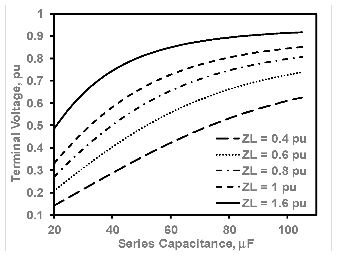
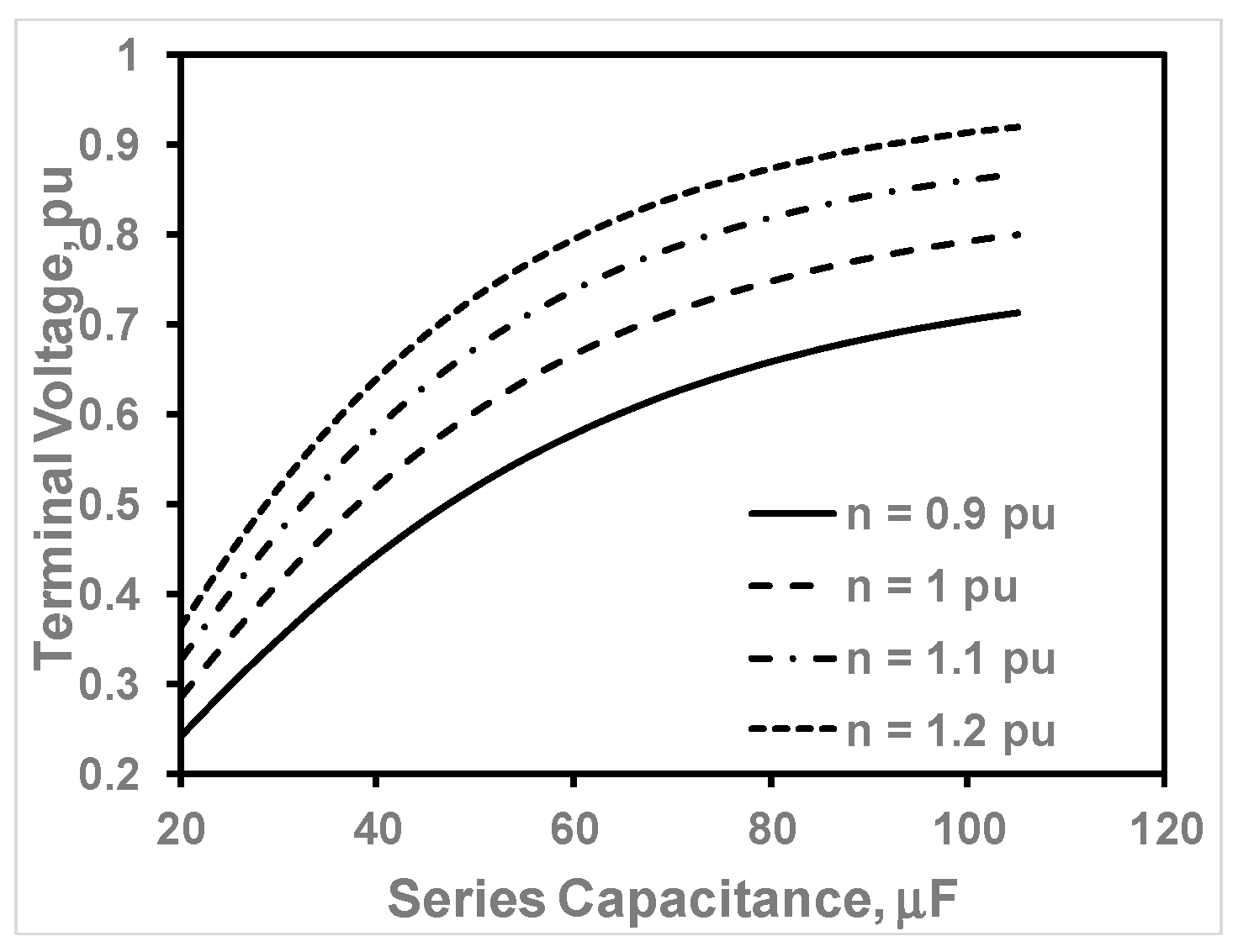
Output terminal voltage is highly affected by changes to the series capacitance with fixed shunt capacitance under different loads and speeds. For example, the variation in terminal voltage when changing the series capacitance between 20 μF and 105 μF, with a shunt capacitance value of 60 μF, under full load and rated speed conditions is between 0.2851 and 0.7998 pu, respectively;

(c)

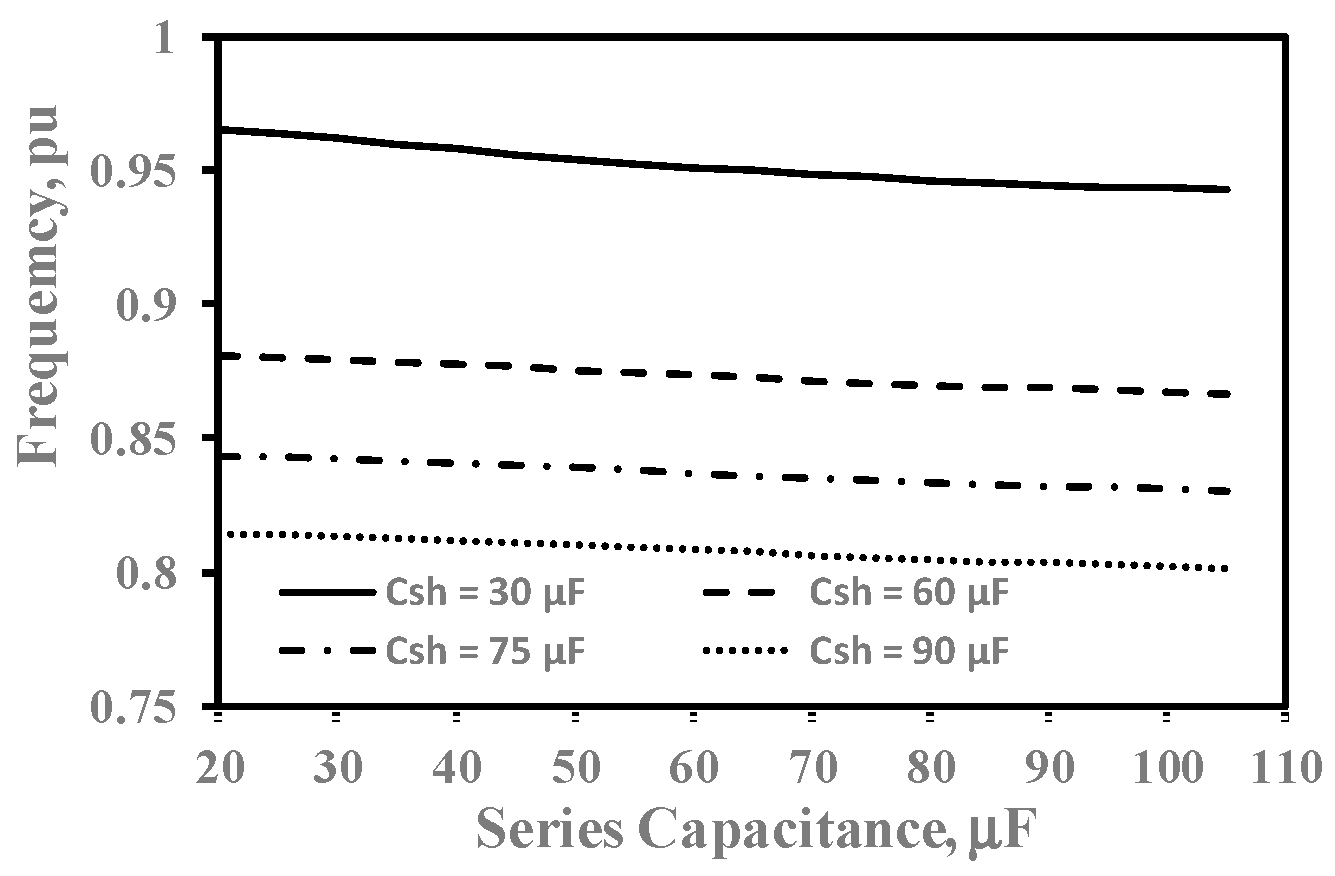
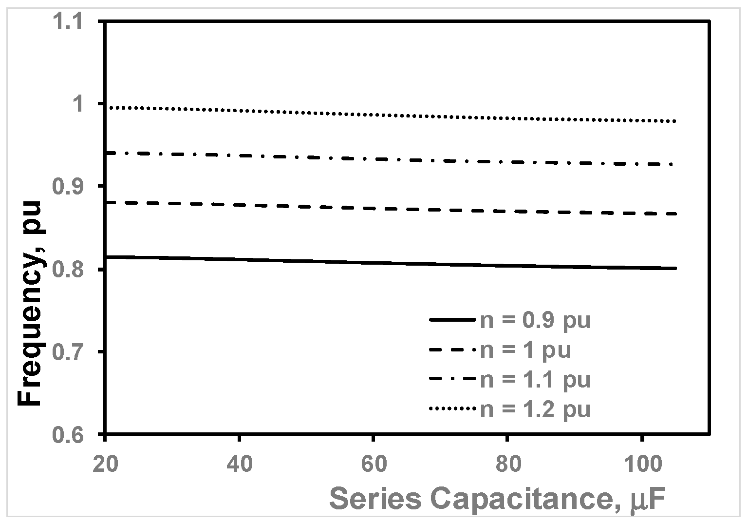
The variation in output frequency is acceptable under different operating conditions with series excitation capacitance but fixed shunt capacitance. For example, the changes in output frequency for the same operating condition provided in the previous point are 0.8808 and 0.8667 pu, respectively;

(d)

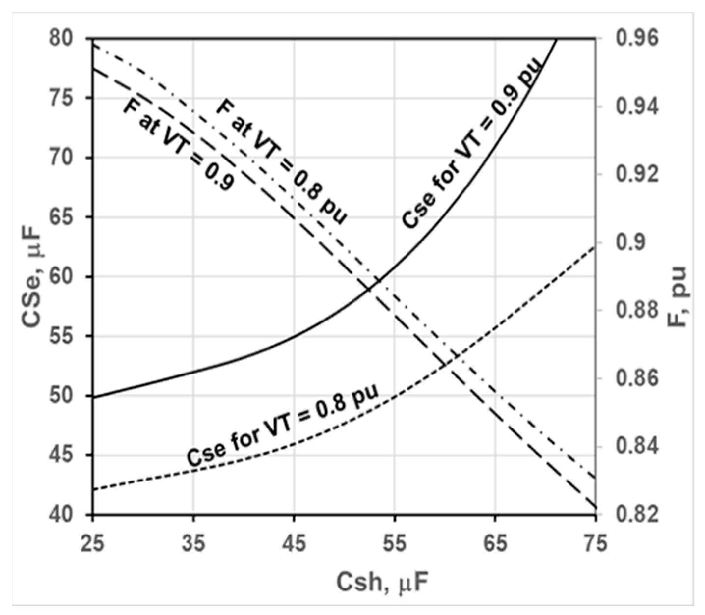
A simply controlled electronic power circuit can be used to achieve fixed terminal voltage and approximately fixed frequency under different operating conditions by selecting the appropriate shunt excitation capacitance value and adjusting the series capacitance.

Figure 10 presents the computed optimum series capacitance for different shunt capacitances to achieve a fixed terminal voltage of 0.9 pu or 0.8 pu. The generator is run at a rated speed of 1 pu and feeds an inductive load with an impedance Z_L of 0.9 pu and a power factor of 0.8. The variations in the output frequency for the same conditions are shown in Figure 10. The required series excitation capacitance to achieve a fixed output voltage of 0.9 pu or 0.8 pu involves increasing the shunt excitation capacitance value. On the other hand, the needed series excitation capacitance to achieve a fixed output voltage of 0.9 pu is higher than that required to acquire a constant voltage of 0.8 for all shunt capacitance values. Concerning the output frequency, a noticeable decrease occurs by increasing the shunt capacitance value. For example, the frequency changes between 0.9513 and 0.8079 pu when changing the shunt capacitance between 25 μF and 80 μF achieves a fixed terminal voltage of 0.9 pu. In addition, the frequency for a fixed terminal voltage of 0.8 pu is higher than a voltage of 0.9 pu for the whole range of shunt capacitance values.

The two curves of the computed optimum series capacitance, with their fixed shunt capacitance of 40 μF, maintain the terminal voltage at 0.95 or 0.9 pu, as shown in Figure 11. The generator during these tests is driven at a rated speed of 1 pu to supply different inductive load impedances with a PF of 0.9. The required series excitation capacitance decreases exponentially with increased load impedance (decreasing the load). For each load impedance, the required capacitance is higher at higher terminal voltages. For example, at a Z_L of 1.2 pu, Cse ≈ 64 μF to achieve a V_T of 0.95 pu, whereas Cse ≈ 45 μF for a V_T of 0.9 pu. From the output frequency curves, the frequency increases non-linearly with Z_L. For the same Z_L value, the frequency is higher for a V_T of 0.9 pu than for a V_T of 0.95 pu.

Figure 12 shows the computed optimum series capacitance with a fixed shunt capacitance of 40 μF, which maintains the terminal voltage at 0.95 or 0.9 pu under variable Z_L with a PF of 0.9 for three different speeds. The output frequency results for the same conditions are presented in Figure 13. The required excitation series capacitance noticeably decreases as the rotational speed increases for the same load. For example, at a load impedance of 1.1 pu, the needed series capacitances for speeds of 0.9, 1, and 1.1 pu are 81, 57, and 39 μF, respectively. As for output frequency behavior, the output frequency increases as the rotor speed increases for each impedance value.

Figure 14 shows three cases of the self-excitation process representing the effect of series and shunt excitation capacitances on SPSEIG voltage buildup. In the first case, the values of C_se and C_sh are 50 μF and 20 μF, respectively. For the second case, the increase in C_se is 5 μF and Csh remains fixed. In the third case, C_se returns to 50 μF and C_sh increases to 25 μF. A small increase in C_se highly affects not only the starting time of voltage buildup but also the amplitude of the voltage. On the other hand, the same increase in C_sh has a minor effect on both voltage amplitude and the initial time of self-excitation. Figure 15 shows the use of C_se to regulate output voltage during load changes. The generator is started at full load, then a step in extra load is applied at 5 s. After 3 s (at time t = 8 s), an appropriate C_se value to regulate the output voltage, with C_sh remaining fixed, is applied. Figure 16 shows C_se regulating output voltage during applied torque changes, corresponding to wind speed variation. As seen in Figure 15 and Figure 16, the terminal voltage of the generator during changes in load or wind speed can be successfully regulated by adjusting the series excitation capacitance.

4. Conclusions

The impact of excitation capacitances on terminal voltage behavior and the frequency of wind-driven self-phase single self-excited induction generators under different conditions was evaluated in this study. Optimum series excitation capacitance values for voltage regulation under load changes and wind speed variation were also computed. Based on the results obtained, it can be concluded that:

• ▪ The increase in C_se has a significant effect on increasing terminal voltage and a minor effect on decreasing output frequency;
• ▪ Increasing C_sh decreases both terminal voltage and frequency;
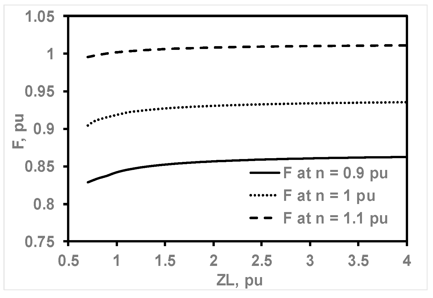
• ▪ For the same C_sh and C_se values, terminal voltage increases by increasing load impedance or speed. The frequency also increases with speed, and is slightly affected by load impedance changes;
• ▪ The optimum C_se for fixed terminal voltage operations under constant load and speed increases with C_sh;
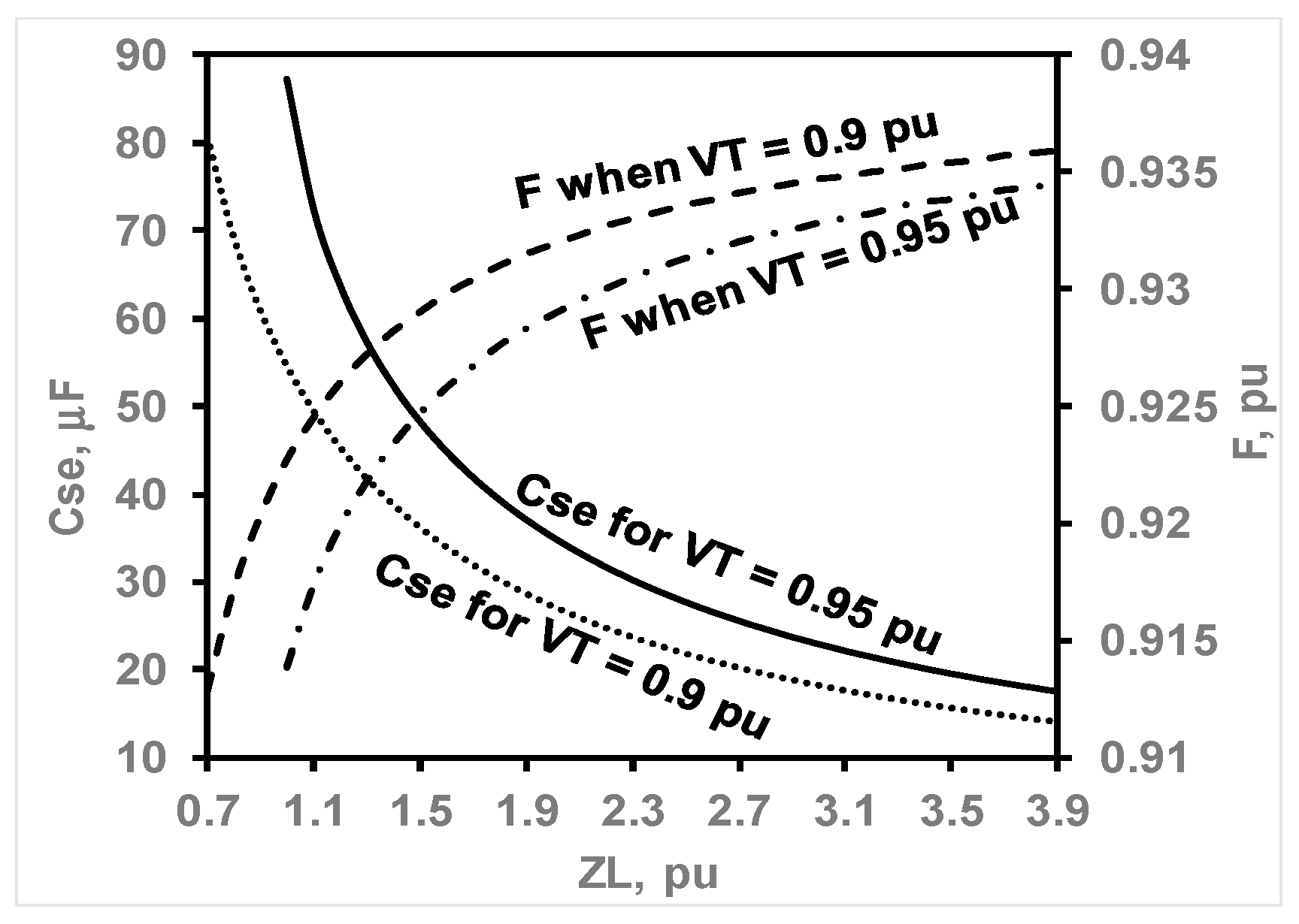
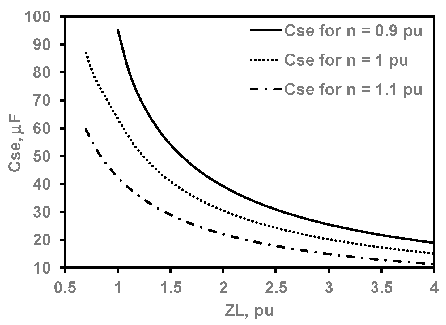
• ▪ The optimum C_se for fixed terminal voltage operation decreases with load impedance and increases with speed;
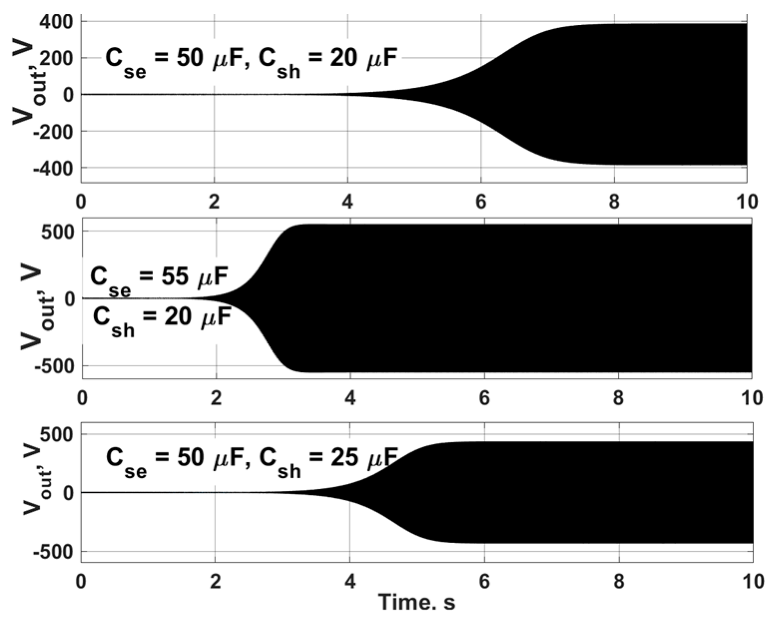
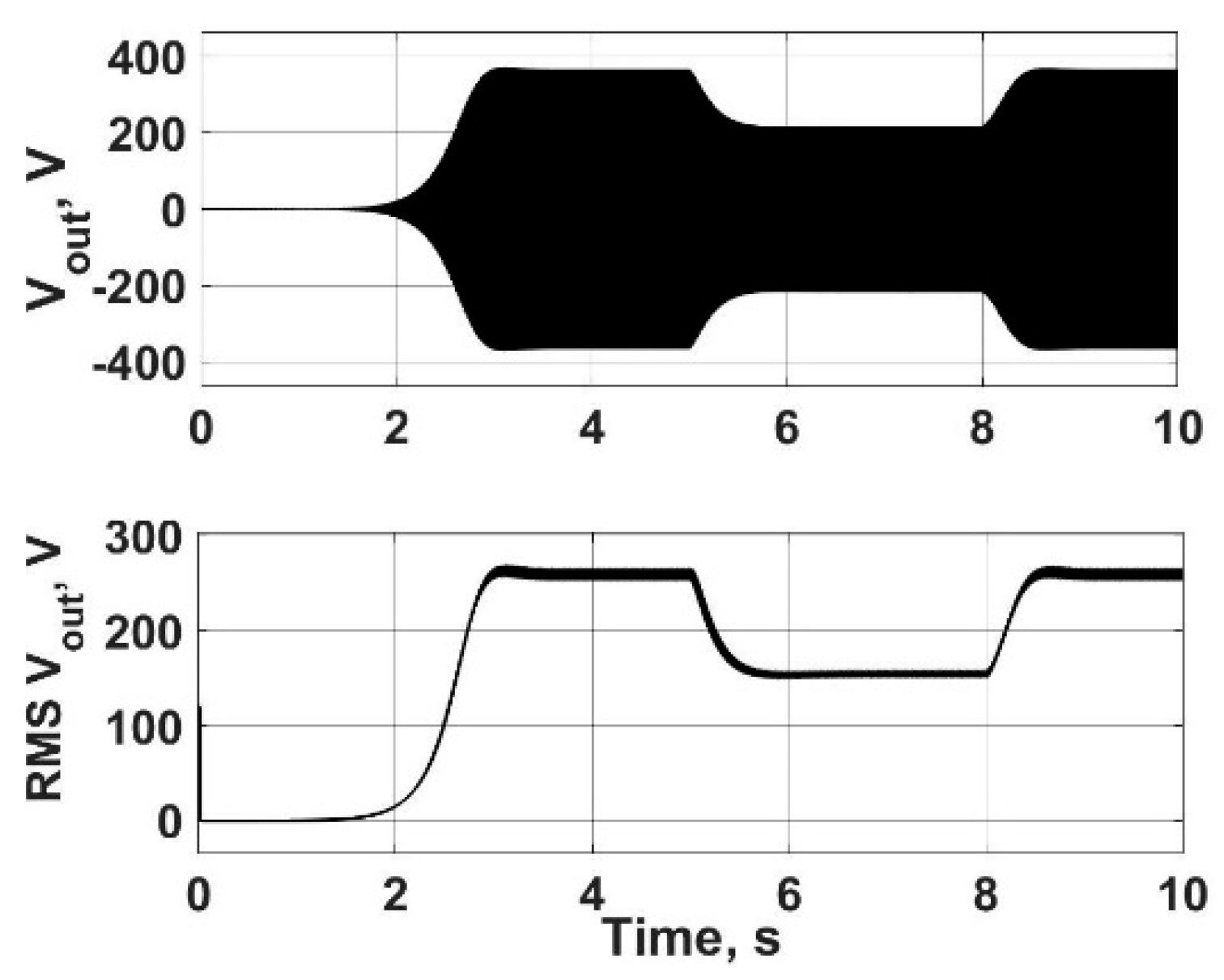
• ▪ During transient operations, a small increase in C_se shortens voltage buildup time and increases the voltage amplitude;
• ▪ Finally, a simple controller for adjusting the series excitation capacitance can successfully regulate the generator’s voltage with acceptable variation in the output frequency.

References

1. Yolcan, O.O. World energy outlook and state of renewable energy: 10-Year evaluation. Innov. Green Dev. 2023, 2, 1–6. [Google Scholar] [CrossRef]
2. Krishna, V.B.M.; Sandeep, V.; Murthy, S.S.; Yadlapati, K. Experimental investigation on performance comparison of self excited induction generator and permanent magnet synchronous generator for small scale renewable energy applications. Renew. Energy 2022, 195, 431–441. [Google Scholar] [CrossRef]
3. Alex, Z.; Kimber, H.M.; Komp, R. Renewable Energy Village Power Systems for Remote and Impoverished Himalayan Villages in Nepal. In Proceedings of the International Conference on Renewable Energy for Developing Countries, Vienna, Austria, 14–16 March 2006. [Google Scholar]
4. Benbouhenni, H.; Ionescu, L.-M.; Mazare, A.-G.; Zellouma, D.; Colak, I.; Bizon, N. Active and reactive power vector control using neural-synergetic-super twisting controllers of induction generators for variable-speed contra-rotating wind turbine systems. Meas. Control 2024, 57, 1–30. [Google Scholar] [CrossRef]
5. Duvvuri, S.S.R.S.; Sandeep, V.; Yadlapati, K.; Krishna, V.B.M. Research on induction generators for isolated rural applications: State of art and experimental demonstration. Meas. Sens. 2022, 24, 1–7. [Google Scholar] [CrossRef]
6. Apostoaia, C. MATLAB-Simulink Model of a Stand-Alone Induction Generator. In Proceedings of the 9th International Conference OPTIM’04, Brasov, Romania, 20–24 May 2004; Transylvania University of Brasov: Brasov, Romania, 2004; Volume 2, pp. 1–8. [Google Scholar] [CrossRef]
7. Krishna, V.B.M.; Sandeep, V.; Narendra, B.K.; Prasad, K.R.K.V. Experimental study on self-excited induction generator for small-scale isolated rural electricity applications. Results Eng. 2023, 18, 2–8. [Google Scholar] [CrossRef]
8. Chakraborty, S.; Samanta, J.; Pudur, R. Experimental analysis of a modified scheme for supplying single-phase remote loads from micro-hydro based three-phase self-excited induction generator. Meas. Sens. 2024, 33, 2–11. [Google Scholar] [CrossRef]
9. Athamnah, I.; Anagreh, Y.; Anagreh, A. Optimization algorithms for steady state analysis of self excited induction generator. Int. J. Electr. Comput. Eng. (IJECE) 2023, 13, 6047–6057. [Google Scholar] [CrossRef]
10. Anagreh, Y.N.; Al-Kofahi, I.S. Genetic Algorithm-Based Performance Analysis of Self-Excited Induction Generator. Int. J. Model. Simul. 2006, 26, 175–179. [Google Scholar] [CrossRef]
11. Domínguez-García, J.L.; Gomis-Bellmunt, O.; Trilla-Romero, L.; Junyent-Ferré, A. Indirect vector control of a squirrel cage induction generator wind turbine. Comput. Math. Appl. 2012, 64, 102–114. [Google Scholar] [CrossRef]
12. Makowski, K.; Leicht, A. Performance Characteristics of Single-Phase Self-Excited Induction Generators with an Iron Core of Various Non-Grain Oriented Electrical Sheets. Energies 2020, 13, 3166. [Google Scholar] [CrossRef]
13. Ion, X.P. A Comprehensive Overview of Single–Phase Self-Excited Induction Generators. IEEE Access 2020, 8, 197420–197430. [Google Scholar] [CrossRef]
14. Leicht, A.; Makowski, K. A single-phase induction motor operating as a self-excited induction generator. Arch. Electr. Eng. 2013, 62, 361–373. [Google Scholar] [CrossRef]
15. Anagreh, Y.N. Matlab-Based Steady-State Analysis of Single-Phase Self-Excited Induction Generator. Int. J. Model. Simul. 2006, 26, 271–275. [Google Scholar] [CrossRef]
16. Sanusi, K.A.; Olatomiwa, L.; Mohammed, A.D.; Sodiq, K.A. Capacitively-Excited Single-phase Asynchronous Generator for Autonomous Applications. Niger. J. Technol. Dev. 2022, 19, 128–135. [Google Scholar] [CrossRef]
17. Arya, S.R.; Maurya, R.; Giri, A.K.; Qureshi, A.; Baladhanautham, C.B. Power quality solutions for effective utilization of single-phase induction generator using voltage source converter. Energy Sources Part A Recovery Util. Environ. Eff. 2020, 1–20. [Google Scholar] [CrossRef]
18. Palwalia, D.K.; Singh, S.P. New Load Controller for Single-phase Self-excited Induction Generator. Electr. Power Compon. Syst. 2014, 57, 1455–1464. [Google Scholar] [CrossRef]
19. Mossad, M.I.; Banakhr, F.A.; Ghoneim, S.S.M.; AbdulFattah, T.A.; Samy, M.M. Self-Regulated Single-phase Induction Generator for Variable Speed Stand-alone WECS. Intell. Autom. Soft Comput. (IASC) 2021, 28, 715–727. [Google Scholar] [CrossRef]
20. Ahshan, R.; Iqbal, M.T. Voltage Controller of a Single Phase Self-excited Induction Generator. Open Renew. Energy J. 2009, 2, 84–90. [Google Scholar] [CrossRef]
21. Ojo, O.; Omozusi, O.; Gonoh, A.G.B. The Operation of a Stand-Alone, Single-Phase Induction Generator Using a Single-Phase, Pulse-Width Modulated Inverter with a Battery Supply. IEEE Trans. Energy Convers. 1999, 14, 526–531. [Google Scholar] [CrossRef]
22. Krause, P.C.; Wasynczuk, O.; Sudhoff, S.D. Analysis of Electric Machinery and Drive Systems, 2nd ed.; Wiley-IEEE Press: Hoboken, NJ, USA, 2002. [Google Scholar]
23. Ojo, O. The Transient and Qualitative Performance of a Self-Excited Single-Phase Induction Generator. IEEE Trans. Energy Convers. 1995, 10, 493–501. [Google Scholar] [CrossRef]
Figure 1. The schematic diagram of two winding SPSEIGs.
Energies 17 03604 g001
Figure 2. (A): q-axis equivalent circuit; (B): d-axis equivalent circuit.
Energies 17 03604 g002
Figure 3. The equivalent circuit of the positive and negative sequence components for SPSEIGs.
Energies 17 03604 g003
Figure 4. Variations in VT with Cse.
Energies 17 03604 g004
Figure 5. Variations in F with Cse.
Energies 17 03604 g005
Figure 6. Variation in VT with Cse for different loads.
Energies 17 03604 g006
Figure 7. Variation in F against Cse for different loads.
Energies 17 03604 g007
Figure 8. Variation in VT vs. Cse at different speeds.
Energies 17 03604 g008
Figure 9. Variation in F vs. Cse at different speeds.
Energies 17 03604 g009
Figure 10. Optimum Cse at different Csh for fixed VT operation under n = 1 pu, ZL = 0.9 pu with PF of 0.8.
Energies 17 03604 g010
Figure 11. Optimum Cse at different ZL with 0.9 PF for a fixed VT operation when n = 1 pu, Csh = 40 μF.
Energies 17 03604 g011
Figure 12. Optimum Cse for fixed VT of 0.9 pu under different ZL, with a PF of 0.9 for different n and a fixed Csh of 40 μF.
Energies 17 03604 g012
Figure 13. Variation in F against ZL for fixed VT operations under different n and a fixed Csh of 40 μF.
Energies 17 03604 g013
Figure 14. The effect of excitation capacitances on the self-excitation of SPSEIGs.
Energies 17 03604 g014
Figure 15. Using Cse to regulate Vout during load changes.
Energies 17 03604 g015
Figure 16. Using Cse to regulate the output voltage during applied torque changes.
Energies 17 03604 g016
Disclaimer/Publisher’s Note: The statements, opinions and data contained in all publications are solely those of the individual author(s) and contributor(s) and not of MDPI and/or the editor(s). MDPI and/or the editor(s) disclaim responsibility for any injury to people or property resulting from any ideas, methods, instructions or products referred to in the content.