Research on Parameter Correction of Distribution Network Model Based on CIM Model and Measurement Data

Abstract

The construction of an energy distribution network can improve the system’s ability to absorb new energy, and its stable and efficient operation has become more and more important. The security and stability analysis of a distribution network needs accurate distribution network model parameters as support. At present, the installation of PMU equipment in China’s distribution network synchronous phase angle measurement unit is limited, which brings challenges to the parameter correction of the distribution network. In this paper, an automatic correction algorithm of distribution network parameters based on the CIM model and measurement data is proposed for the distribution network system without PMU. Firstly, the distribution network topology construction technology based on XML files and key fields of the distribution network is proposed, and the non/small impedance devices (such as switches) are merged and reduced. The breadth-first traversal algorithm is used to verify the connectivity of the constructed topology. Then, based on the topology construction and the least squares method, an iterative parameter correction technique is constructed. Finally, the accuracy and effectiveness of the proposed algorithm are verified in a standard IEEE 33-bus system distribution network and an example of the China Southern Power Grid. The topology connections constructed based on the CIM model have significantly enhanced the efficiency of parameter correction.

1. Introduction

The uncertainty of new energy generation and load can jeopardize the stable operation of the power system [1,2]. As the end link of the power system, the distribution network converts the electrical energy from the high-voltage transmission lines into low-voltage electrical energy and transmits it to the users, carrying the important mission of supplying power directly to the users [3,4]. The difficulty and complexity of distribution network control are high, and in order to ensure the safety, reliability, and stability of the distribution network, accurate distribution network line parameters are the foundation [5]. However, at present, manually woven data has a wide range of applications [6,7]. Grid operators often use theoretical calculations or offline measurements to obtain line parameters according to the type of conductor and geometric parameters, which is likely to lead to analyzing the incorrect line parameters used by the operator. In some cases, the error between the adopted model parameters and the real parameters may reach as much as 25–30% [8], which adversely affects the security and stability analysis of distribution networks.

Scholars at home and abroad have conducted some research on the correction of distribution network line parameters. The literature [9] proposed a deep and shallow neural network with physical consistency to create virtual nodes to simulate missing quantities for distribution network parameter identification. The literature [10] proposed a variance-based reweighted nonlinear least squares method for parameter identification based on the SCADA system. The literature [11] combines synchronized and asynchronized measurements for parameter identification based on an alternating direction multiplier method. The literature [12] used inverse tidal equations for parameter identification by reconstructing the distribution network weighted Laplace matrix. The literature [13] proposed the ‘PaToPaEM’ framework based on measurement errors and used maximum likelihood estimation to solve for parameters and topology. The literature [14] utilizes end-of-line data for joint topology and parameter identification. The algorithms also have O(|V|³) computational complexity.

The current research mostly focuses on measurement data-driven identification methods, which do not fully utilize the original topology information. The Common Information Model (CIM) of the distribution network contains topological information of the distribution network, and the full utilization of topological information will be beneficial for improving the accuracy of line parameter identification. The literature [15] utilized the correlation coefficient method to determine the phase sequence and node connectivity of LV distribution networks. The literature [16] constructs the topology of LV distribution networks based on principal component analysis and graph theory. The literature [17] performs node correlation analysis and topology modeling based on Markov random field. The literature [18] proposed a topology identification model based on mixed integer quadratic programming (MIQP) that can identify topologies with weighted least squares (WLS) with measurement residuals. These studies provide a basis for the construction of topology models for distribution networks, while the algorithm for correcting line parameter identification based on the topology model is yet to be further investigated.

PMU (Phasor Measurement Unit) is a high-precision power system monitoring device that can synchronously acquire voltage and current phasor data. Due to its limited installation, this paper proposes a distribution network line parameter correction method based on the CIM model and measurement data for distribution network systems without PMU. The method consists of three stages. Firstly, the topology of the distribution network is constructed based on the CIM model and combined with the key fields, and the topology reduction is performed for small impedance lines. Then, combined with the constructed topology of the network, the identification and correction of the distribution network parameters are performed based on the measurement data using the least-squares algorithm and the improved Newton’s method. By integrating the CIM model with measurement data, accurate topological connections were established as a foundation, which improved the precision and efficiency of parameter identification and correction, thereby achieving precise construction of the distribution network topology. Finally, this paper carries out an experimental simulation by using the IEEE 33-bus case and the actual data of Southern Grid to validate the feasibility and accuracy of the method.

2. CIM-Based Distribution Network Topology Construction

2.1. Introduction to CIM and XML Files

Currently, CIM is commonly used by electric power enterprises to describe various data on power system operations, including grid equipment attributes, connection relationships between equipment, etc. CIM follows the IEC 61970 standard [19] and uses the Extensible Markup Language and Resource Description Framework to describe equipment in detail [20,21,22,23], which is used for exchanging data and information in an offline situation.

The CIM contains a variety of data in the distribution network, such as information about substations, distribution lines, transformers, switches, and other equipment, as well as their relationships and attributes. The IEC 61970 standard defines the structure and attributes of an XML file to ensure that the file can be parsed and processed by different applications [24].

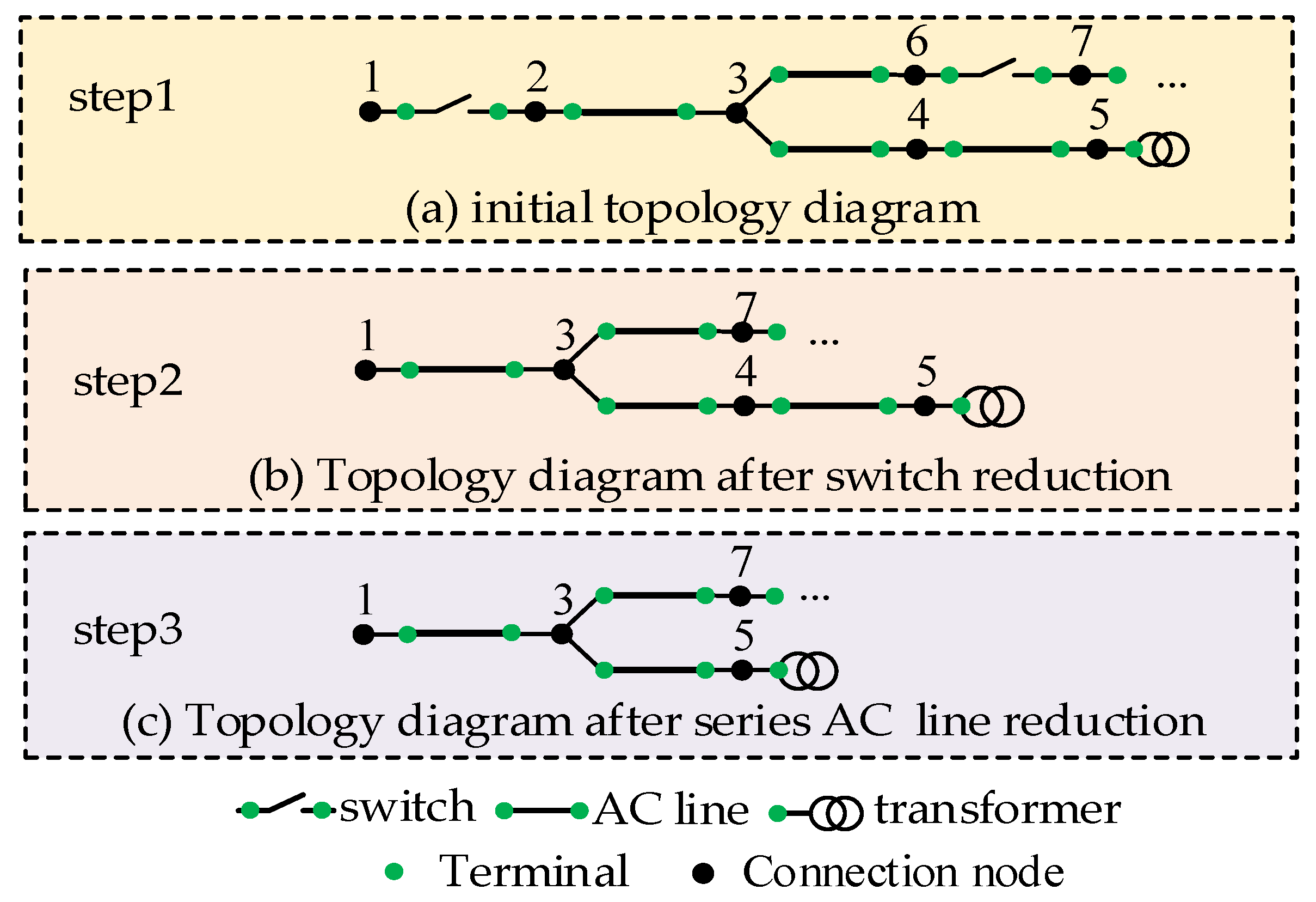
2.2. Topology Construction and Topology Reduction

The key fields used for topology construction in CIM/XML files contain information such as connection nodes, terminals, switches, and device parameters. By interpreting and analyzing the key fields, the topology model of the distribution network is constructed.

The flowchart of topology construction and topology reduction is shown in Figure 1. The first step is to parse the key fields of the XML file describing the equipment of the distribution network to obtain information on the distribution network equipment. Then, the topology construction and topology reduction are performed based on the information of the equipment connections. Then, the missing parameters are supplemented, and, finally, the topology checking is performed, and the topology model is outputted.

The topology reduction of the build consists of three main steps in Figure 2. Step 1: Firstly, key equipment information is extracted, including switch class, AC line class, transformer winding class, and other equipment. By analyzing the connection terminals and connection nodes of these key devices, the initial topology connectivity diagram is obtained, as shown in Figure 2a. Step 2: Due to the very small resistance value of the switch class devices, it is necessary to reduce this class of devices in the process of topology construction, and the schematic diagram of the reduction result is shown in Figure 2b. Step 3: Series-connected AC connecting wires are widely present in the original topology model, and these series-connected AC connecting lines will lead to the construction of the topology nodes, of which there are too many. Therefore, this paper, through the impedance value summing method, will be a series AC line reduction, reducing the number of topology nodes and reducing the final topology graph, as shown in Figure 2c.

2.3. Missing Parameters and Abnormal Data Replacement

Currently, topological model operation mainly relies on manual labor, which requires technicians to maintain the engineering management system or GIS. The manually maintained topological model requires a lot of manual operation and is prone to errors, which leads to the problem of parameter anomalies, such as misspellings, missing data, and so on. Therefore, there is a need to identify and correct such problems. In this design, due to the anomalies and missing data in some of the data within the XML file, which includes the data required for topology construction, they are identified and corrected.

Parameters missing location identification and parameter supplementation methods based on similar devices are first fixed by finding and identifying the missing and abnormal items in the data and then correcting and supplementing them. The identification and correction of missing and abnormal data can improve the accuracy and reliability of the data.

3. Distribution Network Line Parameter Correction

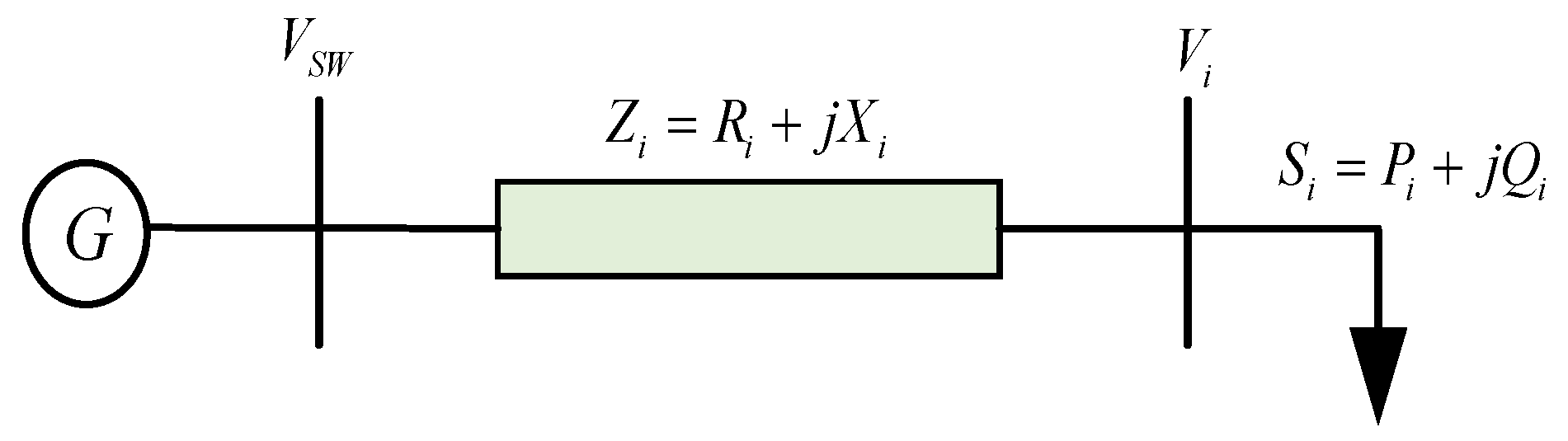
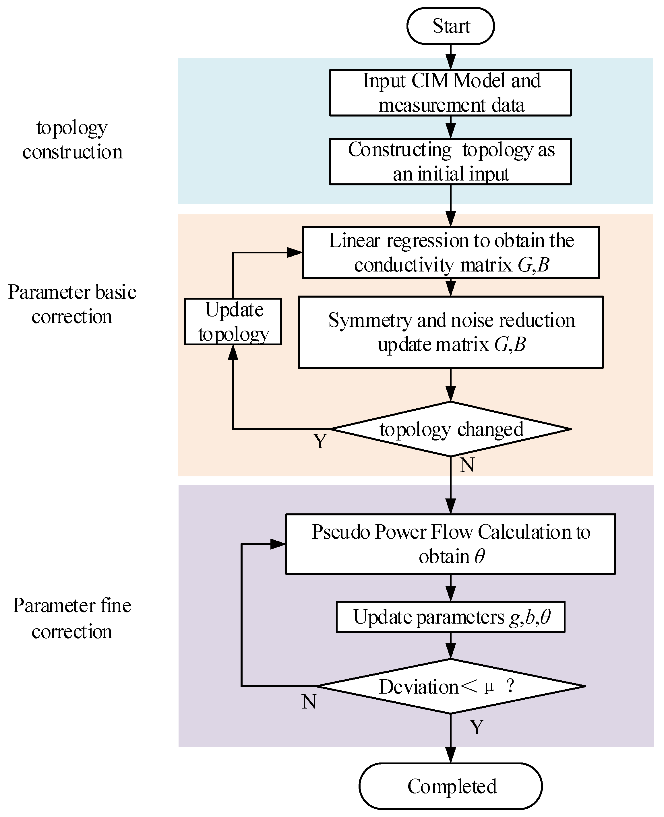
3.1. Distribution Network Parameter Basis Correction

This section describes the principles of a least squares-based foundation correction of distribution network line parameters.

The least squares method determines the function model that best matches the data points by fitting the data points. The least squares method obtains the best parameter estimates by minimizing the sum of squares of the residuals between the actual observations and the predicted values. The process can be implemented using various types of numerical optimization algorithms, e.g., iterative methods or gradient descent algorithms.

In Figure 3, if the voltage as well as the power of a single measurement point is known, the resistance and reactance values of the line can be calculated. If multiple measurement points of data are obtained, the least squares estimates of the line resistance and reactance can be estimated based on the least squares method.

The current equation in the polar coordinate system of a distribution network with n buses is shown in Equation (1).

$$\{\begin{array}{c}{p}_i=v_i{\displaystyle {\sum }_{j=1}^n{v}_j(G_{ij}\cos {\theta }_{ij}+B_{ij}\sin {\theta }_{ij})}\\ q_i=v_i{\displaystyle {\sum }_{j=1}^n{v}_j(G_{ij}\sin {\theta }_{ij}-B_{ij}\cos {\theta }_{ij})}\end{array}$$

(1)

where i and j mean the bus number, p_i, q_i are the active power and reactive power injected into bus i, respectively, v_i is the voltage magnitude of the bus i, θ_ij is the phase angle difference of the voltage between buses i and j, and G_ij, B_ij are the mutual conductance and mutual conductance between buses i and j, respectively.

To find the line parameters and phase angle parameters (g, b, and θ) that satisfy the tidal equation, the least squares method can be used. The principle of least squares is shown in Equation (2):

$$\begin{array}{c}\underset{[G_{ij}],[B_{ij}],\theta }{min}{\displaystyle \sum _{i=1}^n{(p_i-v_i{\displaystyle {\sum }_{j=1}^n{v}_j(G_{ij}\cos {\theta }_{ij}+B_{ij}\sin {\theta }_{ij})})}^2}\\ +{\displaystyle \sum _{i=1}^n{(q_i-v_i{\displaystyle {\sum }_{j=1}^n{v}_j(G_{ij}\sin {\theta }_{ij}-B_{ij}\cos {\theta }_{ij})})}^2}\end{array}$$

(2)

Transforming the nodal voltage magnitude in Equation (1) to the right-hand side of the equation reduces it to the form shown in Equation (3).

$$\begin{array}{c}{p}_i/v_i={\displaystyle {\sum }_{j=1}^n{v}_j(G_{ij}\cos {\theta }_{ij}+B_{ij}\sin {\theta }_{ij})}\\ q_i/v_i={\displaystyle {\sum }_{j=1}^n{v}_j(G_{ij}\sin {\theta }_{ij}-B_{ij}\cos {\theta }_{ij})}\end{array}$$

(3)

Equation (3), written in the form of a matrix, can be changed to Equation (4).

$$\{\begin{array}{c}\widehat{p}=\tilde{G}\widehat{v}\\ \widehat{q}=-\tilde{B}\widehat{v}\end{array}$$

(4)

$$\{\begin{array}{c}\widehat{p}=[p/v]=[p_1/v_1\cdots p_n/v_n{]}^T\\ \begin{array}{c}\widehat{q}=[q/v]=[q_1/v_1\cdots q_n/v_n{]}^T\\ \widehat{v}=[v]={[v_1\cdots v_n]}^T\begin{array}{cc}\begin{array}{cc}& \end{array}& \end{array}\end{array}\end{array}$$

(5)

The matrix in Equation (4) contains the active power, reactive power, and voltage magnitude information of all buses, and in Equation (4), it denotes the approximation of the conductance and conductivity matrix of the distribution network buses, expressed as Equation (6).

$$\begin{array}{l}{\tilde{G}}_{ij}=G_{ij}\cos {\theta }_{ij}+B_{ij}\sin {\theta }_{ij}\\ {\tilde{B}}_{ij}=-G_{ij}\sin {\theta }_{ij}+B_{ij}\cos {\theta }_{ij}\end{array}$$

(6)

The operational characteristics of the distribution network contain the following three points: (1) the R/X ratio is large, generally close to or greater than 1; (2) the nodal voltage magnitude tends to be close to 1 p.u.; and (3) the phase angle difference between the two ends of the line is very small [25]. According to the operational characteristics of the distribution network, it can be seen that the voltage phase angle difference between the two buses of any branch is sinθ_ij ≈ θ_ij. Therefore, it can be approximated as sinθ_ij ≈ 0, cosθ_ij ≈ 1, and the approximation of and can be expressed as Equation (7):

$$\begin{array}{l}{\tilde{G}}_{ij}=G_{ij}+{\theta }_{ij}{B}_{ij}\\ {\tilde{B}}_{ij}=B_{ij}-{\theta }_{ij}{G}_{ij}\end{array}$$

(7)

If there are a total of M sets of bus measurement data, the linear regression method can be utilized to linearly regress the matrix and to obtain the following:

$$\begin{array}{l}\tilde{G}=[\widehat{P}]{[V]}^T{([V]{[V]}^T)}^{-1}\\ \tilde{B}=-[\widehat{Q}]{[V]}^T{([V]{[V]}^T)}^{-1}\end{array}$$

(8)

$$\{\begin{array}{c}\widehat{P}=[{\widehat{p}}_1\cdots {\widehat{p}}_M]=[{[p/v]}_1\cdots {[p/v]}_M]\\ \begin{array}{c}\widehat{Q}=[{\widehat{q}}_1\cdots {\widehat{q}}_M]=[{[q/v]}_1\cdots {[q/v]}_M]\\ V=[{\widehat{v}}_1\cdots {\widehat{v}}_M]=[{[v]}_1\cdots {[v]}_M]\begin{array}{cc}& \end{array}\end{array}\end{array}$$

(9)

According to the operating characteristics of the power grid, it is necessary to ensure that the conductivity matrix is a symmetric matrix, which is symmetrically processed, as shown in Equation (10), and denotes symmetry.

$$\begin{array}{l}{\tilde{G}}_s=(\tilde{G}+{(\tilde{G})}^T)/2\\ {\tilde{B}}_s=(\tilde{B}+{(\tilde{B})}^T)/2\end{array}$$

(10)

Due to the measurement data and linear regression errors resulting in the presence of noise in the conductance matrix, the conductance matrix needs to be noise reduction. In this paper, we use the contribution of mutual conductance to self-conductance to produce a judgment, i.e.,

$$\gamma (i,j)={\displaystyle \frac{\left|G_{ij}\right|}{\left|G_{ii}\right|}}$$

(11)

where G_ij is the mutual conductance between bus i and bus j, and G_ii is the self-conductance of bus i.

When γ(i, j) is less than the set threshold, the branch is considered a noise branch and needs to be removed. If the topology model does not change before and after noise reduction, the line parameters obtained from the base correction are the output.

3.2. Distribution Network Parameter Fine Correction

After the basic correction, the obtained line parameters still have a large deviation from the actual values. In order to reduce the deviation, with the known nodal voltage magnitude v, active power p, and reactive power q, the line parameters g and b obtained from the basic identification correction of the line parameters in Section 3.1 are taken as the initial values to be brought into the improved Newton–Raphson equations, and iteratively solved for more accurate line parameters [26]. Additionally, the pseudo power flow calculation method is employed to enhance convergence using the estimated g and b and measured power p and q to obtain voltage phase angle information. The phase angle obtained from the pseudo power flow calculation replaces the θ in each iteration to assist convergence.

According to the improved Newton–Raphson method, the parameter correction model can be obtained as follows:

$$\left[\begin{array}{c}\Delta P\\ \Delta Q\end{array}\right]=\left[\begin{array}{c}\begin{array}{ccc}{\displaystyle \frac{\partial P}{\partial g}}& {\displaystyle \frac{\partial P}{\partial b}}& {\displaystyle \frac{\partial P}{\partial \theta }}\end{array}\\ \begin{array}{ccc}{\displaystyle \frac{\partial Q}{\partial g}}& {\displaystyle \frac{\partial Q}{\partial b}}& {\displaystyle \frac{\partial Q}{\partial \theta }}\end{array}\end{array}\right]\times \left[\begin{array}{c}\Delta g\\ \Delta b\\ \Delta \theta \end{array}\right]$$

(12)

where ΔP and ΔQ are the active and reactive deviation at each bus during the iteration, respectively.

When there is only one set of measurement data, the results obtained are unreliable due to measurement errors and the characteristics of the underdetermined system. It is necessary to determine the minimum number of samples N, i.e., the number of independent equations is equal to the number of variables when a unique solution can be obtained. For a distribution network with n buses and m branches, the number of unknowns g, b, and θ is 2m + N(n − 1), and the number of independent equations is 2nN, which needs to satisfy 2nN ≥ 2m + N(n − 1), so the minimum number of samples can be satisfied with Equation (13):

$$N\ge {\displaystyle \frac{2m}{n+1}}$$

(13)

The Jacobi matrix obtained from N samples is usually not a square matrix, and the generalized inverse of the Jacobi matrix is solved [27]. From Equation (14), the refined discriminative modified solution for g, b, and θ is shown in Equation (15):

$$\left[\begin{array}{c}\Delta g\\ \Delta b\\ \Delta \theta \end{array}\right]={\left[\begin{array}{c}\begin{array}{ccc}{\displaystyle \frac{\partial P}{\partial g}}& {\displaystyle \frac{\partial P}{\partial b}}& {\displaystyle \frac{\partial P}{\partial \theta }}\end{array}\\ \begin{array}{ccc}{\displaystyle \frac{\partial Q}{\partial g}}& {\displaystyle \frac{\partial Q}{\partial b}}& {\displaystyle \frac{\partial Q}{\partial \theta }}\end{array}\end{array}\right]}^{†}\cdot \left[\begin{array}{c}\Delta P\\ \Delta Q\end{array}\right]$$

(14)

$${\left[\begin{array}{c}g\\ b\\ \theta \end{array}\right]}^{k+1}={\left[\begin{array}{c}g\\ b\\ \theta \end{array}\right]}^k+\left[\begin{array}{c}\Delta g\\ \Delta b\\ \Delta \theta \end{array}\right]$$

(15)

where $†$ denotes the generalized inverse, and k denotes the number of iterations. The iteration is stopped when ΔP and ΔQ satisfy the convergence condition.

The calculation of each element of the Jacobi matrix will be expanded below. For a given sample of measurements, the Jacobi matrix can be divided into six partition matrices: A, B, C, E, F, and H, as shown below:

$$\left[\begin{array}{c}\begin{array}{ccc}{\displaystyle \frac{\partial P}{\partial g}}& {\displaystyle \frac{\partial P}{\partial b}}& {\displaystyle \frac{\partial P}{\partial \theta }}\end{array}\\ \begin{array}{ccc}{\displaystyle \frac{\partial Q}{\partial g}}& {\displaystyle \frac{\partial Q}{\partial b}}& {\displaystyle \frac{\partial Q}{\partial \theta }}\end{array}\end{array}\right]=\left[\begin{array}{c}\begin{array}{ccc}A& B& C\end{array}\\ \begin{array}{ccc}E& F& H\end{array}\end{array}\right]$$

(16)

From the tidal equation, we can obtain Equation (17).

$$\{\begin{array}{c}{p}_i={\displaystyle {\sum }_{j=1}^n(({v_i}^2-v_i{v}_j\cos {\theta }_{ij})G_{ij}-v_i{v}_j\sin {\theta }_{ij}{B}_{ij})}\\ q_i={\displaystyle {\sum }_{j=1}^n(}-v_i{v}_j\sin {\theta }_{ij}{G}_{ij}-({v_i}^2-v_i{v}_j\cos {\theta }_{ij})B_{ij})\end{array}$$

(17)

For branch power partition matrix is given by the above Equation:

$$\begin{array}{l}{A}_{ij}=-F_{ij}=v_i^2-v_i{v}_j\cos {\theta }_{ij}\\ B_{ij}=E_{ij}=v_i{v}_j\sin {\theta }_{ij}\end{array}$$

(18)

For the power angle partition matrix, the relationship between the bus-injected power and voltage data and the voltage phase angle is represented. Since the phase angle θ cannot be expressed linearly, the partial derivatives are used to express and derive Equation (19).

$$\begin{array}{l}{C}_{ij}=\{\begin{array}{c}{v}_i{\displaystyle {\sum }_{j,j\ne i}^n{v}_j(-G_{ij}\sin {\theta }_{ij}+B_{ij}\cos {\theta }_{ij}),i=j}\\ v_i{v}_j(G_{ij}\sin {\theta }_{ij}-B_{ij}\cos {\theta }_{ij}),i\ne j\begin{array}{cc}& \end{array}\end{array}\\ H_{ij}=\{\begin{array}{c}{v}_i{\displaystyle {\sum }_{j,j\ne i}^n{v}_j(G_{ij}\cos {\theta }_{ij}+B_{ij}\sin {\theta }_{ij}),i=j}\\ -v_i{v}_j(G_{ij}\cos {\theta }_{ij}+B_{ij}\sin {\theta }_{ij}),i\ne j\end{array}\end{array}$$

(19)

3.3. Overall Flowchart of the Algorithm

Figure 4 is the overall flow chart of the algorithm, which includes three links: topology construction, parameter base correction, and parameter fine correction.

4. Case Study

In order to verify the effectiveness of the distribution network topology construction method proposed in this paper, this section is tested in a real case of the Southern Power Grid. The parameter correction link uses a typical medium voltage distribution network of the IEEE 33-bus case for the validation test.

4.1. A 10 kV Distribution Network of the Southern Power Grid

4.1.1. Interpretation of CIM Models

The key fields in the CIM/XML file of a feeder of the Southern Power Grid are parsed, and the parsed device types are shown in

Table 1. Equipment class name and type.

No.	Type	CIM Model Class Name
1	AC LINE	Circuit
2		ACLineSegment
3		Junction
4	SWITCH	Breaker
5		LoadBreakSwitch
6		Disconnector
7		GroundDisconnector
8		Fuse
9	TRANSFORMER	PowerTransformer
10	TERMINAL	Terminal
11	NODE	ConnectivityNode

. The table contains the Chinese class names of the devices required for topology construction, the class names of the CIM, and the abbreviations of the CIM categories.

4.1.2. Topology Construction and Reduction

Assuming the impedance of the switches is negligible, the topology constructed based on the CIM model is highly consistent with the actual operational conditions of the power grid, and there are no external interferences in the system. The topology of the distribution network is constructed by first reading and collating the data within the CIM/XML file and then finding the required devices to be processed. As can be seen in Figure 2, in order to obtain the topology of the distribution network, only the information on the terminals and connection nodes of each device is required. Firstly, the key electrical devices required are identified, including switches, overhead lines, cables and electrical connections, and transformer windings, and then the terminals and connection nodes of these devices are found separately. The topology is constructed based on the topological connection relationships, and the impedance values of the AC lines are calculated based on their type and length.

A CIM/XML file of a Southern Power Grid in this example is processed to obtain information on 136 switches, 398 AC lines, and 59 transformers.

Due to the existence of some missing data and errors within the XML file, it will be supplemented and corrected to test the topology. This paper uses the breadth-first traversal algorithm to test the topology; after verification can be obtained, the number of traversed nodes and the total number of nodes is known, proving the connectivity of the topology. The connectivity of the topology can also be observed as shown in Figure 5a.

In order to test the connectivity of the reduced topology, this paper also performs breadth-first traversal of the reduced 180-line Branch data file format, which results in a total of 181 nodes, which are traversed, and its topological model is drawn to obtain Figure 5b.

In conclusion, constructing the distribution network topology based on the CIM model ensures high accuracy through the standardization of equipment components and their interconnections. Compared to actual grid diagrams, the topological connections are almost entirely consistent. The standardization provided by the CIM model significantly enhances the applicability and reliability of the algorithm.

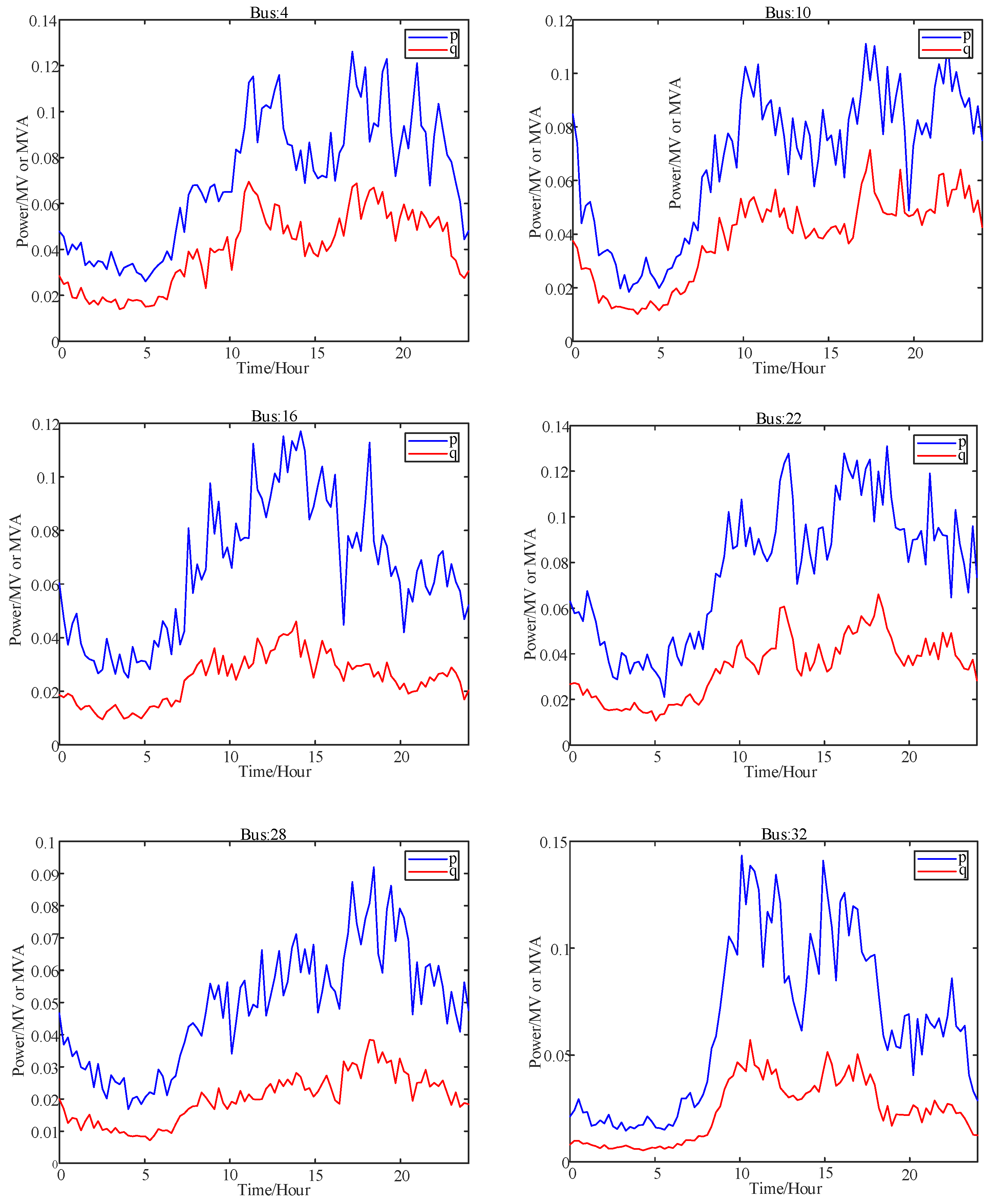
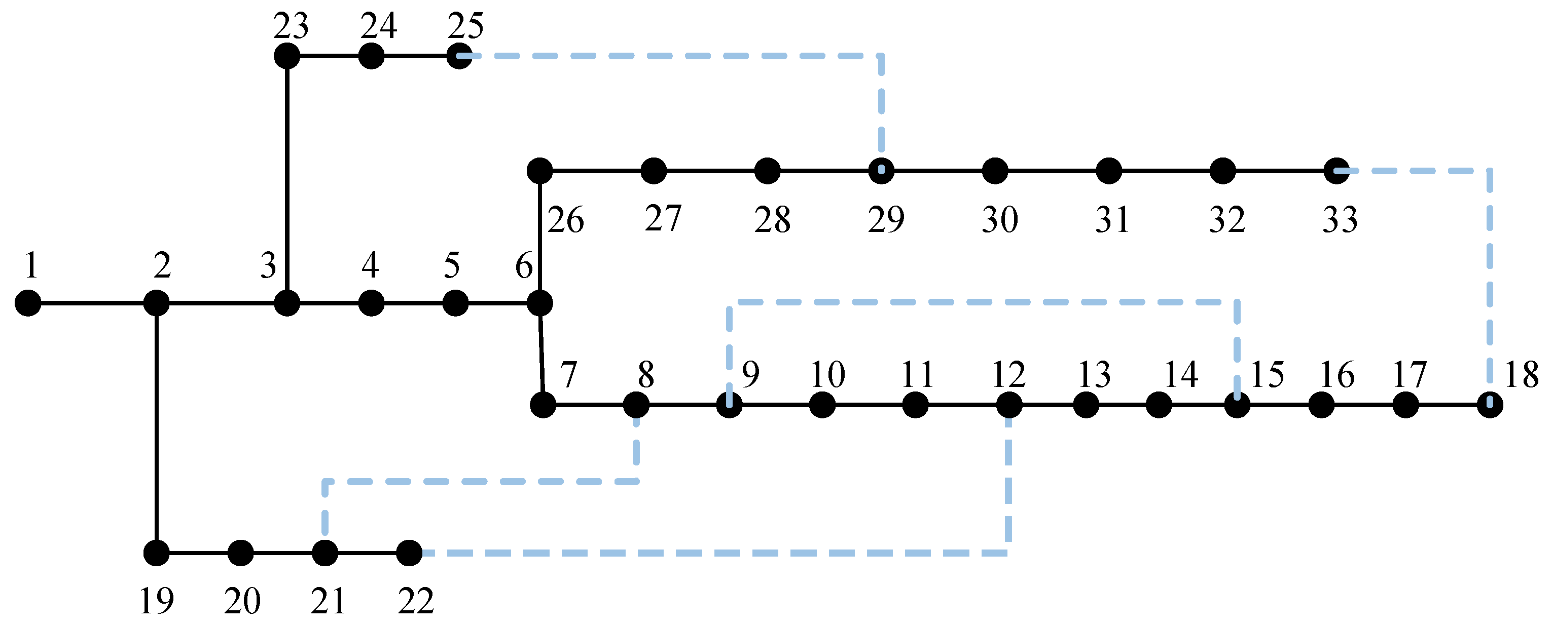
4.2. IEEE 33-Bus Arithmetic Example

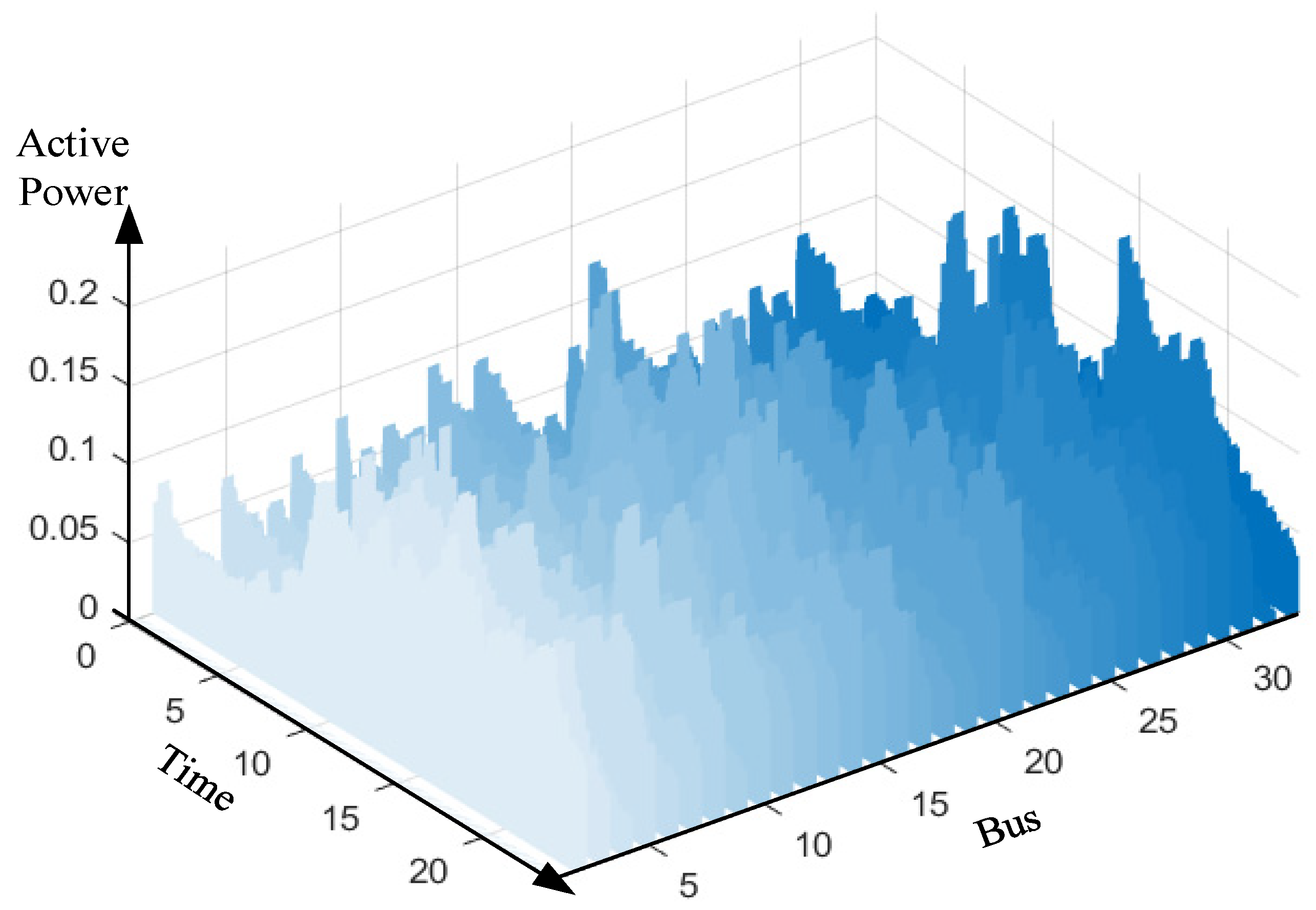
4.2.1. Data Sources

The data utilized in this study is sourced from The Research Perspective Ltd., which collected specific load data of Irish residential users. Since this dataset originates from an actual distribution network system, there are inherent discrepancies between the actual system and the distribution network model used in this paper, leading to differences in specific load values. To better simulate the power flow distribution of the example distribution network, this study retains the shape characteristics of the load curves and the power factor features from the original dataset and adjusts the values based on the anticipated reasonable values for the specific example distribution network.

Specifically, for a distribution system with n buses, there should be n − 1 sets of active power p and reactive power q curves. An easy way to construct load curves for the buses is to sum the load curves of several residents. In this paper, we divide 1000 residents equally into n − 1 groups and obtain the original n − 1 load curves with a half-hour sampling frequency. For times t that are not on the hour or half-hour, linear interpolation between the hour or half-hour points is used. The specific data construction method is shown in Equation (20).

$$\begin{array}{l}{P}_{i,t,new}={\displaystyle \frac{p_{i,t}}{\max (p_{i,t},t)}}\cdot P_0\cdot (1+R_1)\\ Q_{i,t,new}={\displaystyle \frac{p_{i,t}}{\max (p_{i,t},t)}}\cdot Q_0\cdot (1+R_2)\end{array}$$

(20)

In the equation, P_i,t,new and Q_i,t,new represent the active power and reactive power output of bus i at time t, respectively. P_i,t denotes the original user load of bus i, and max(p_i,t, t) represents the maximum load value of the bus. P₀ and Q₀ denote the anticipated maximum active power and reactive power of the distribution network system, respectively. R₁ and R₂ are additional deviations following an independent normal distribution.

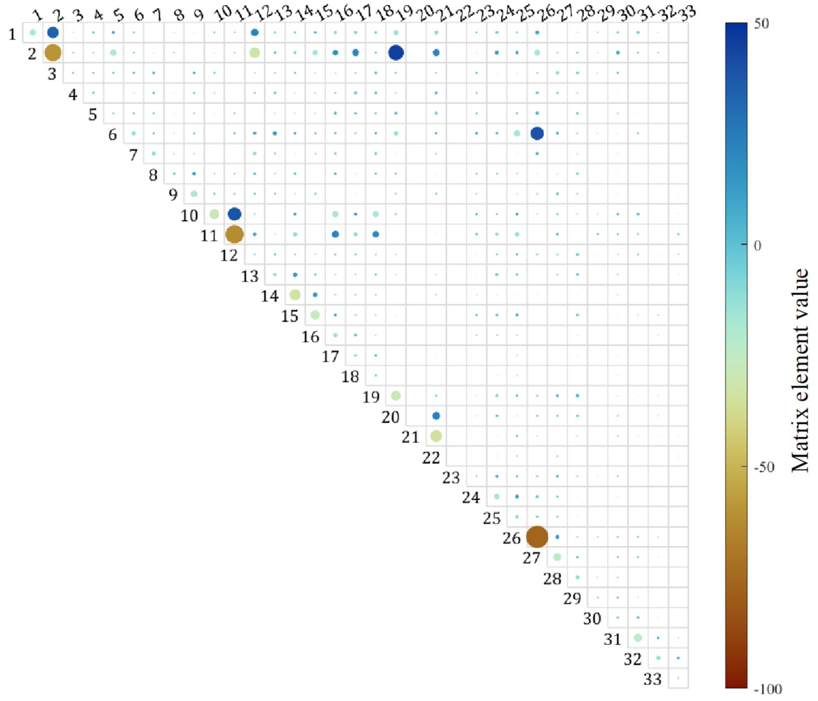
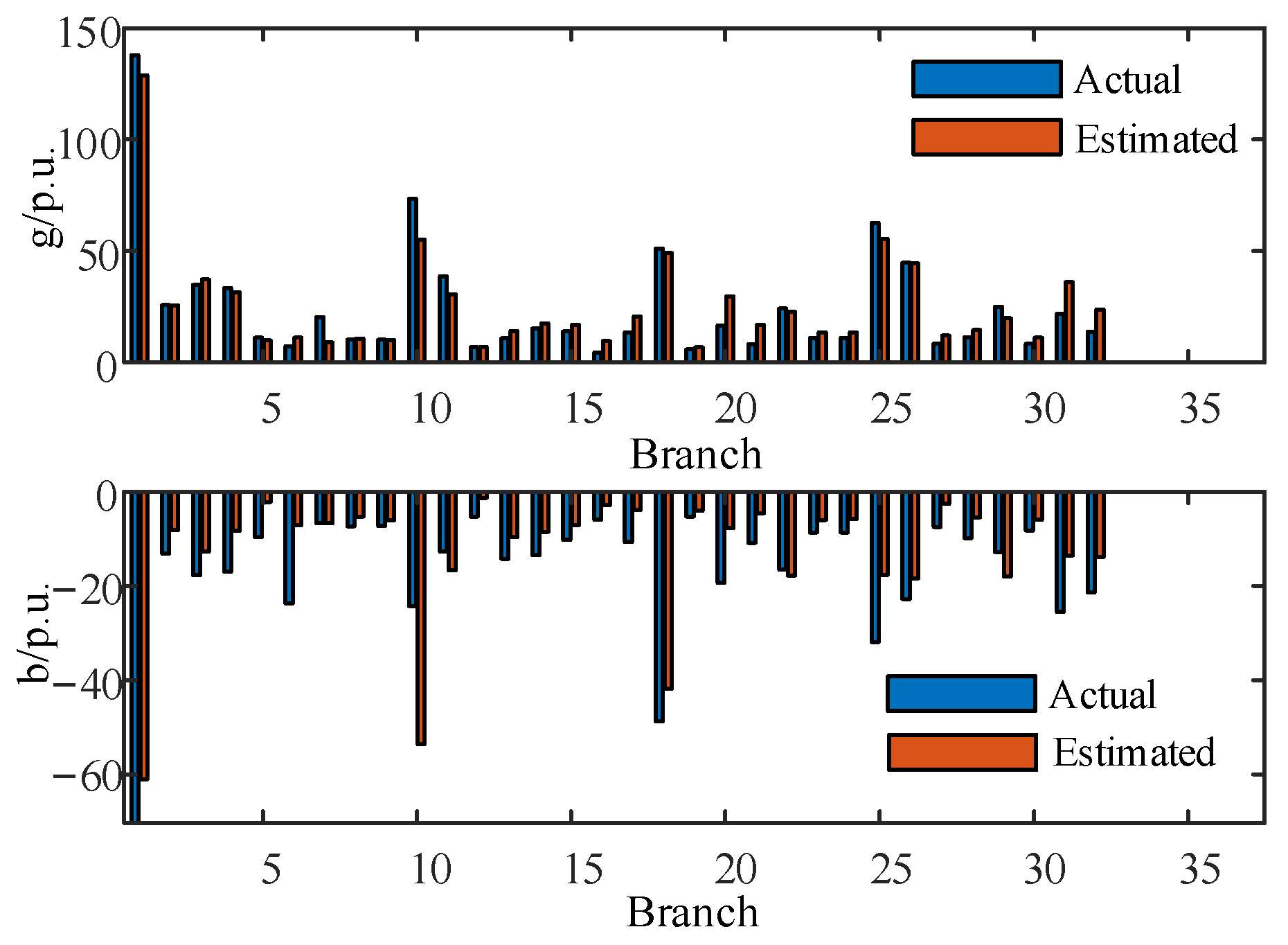
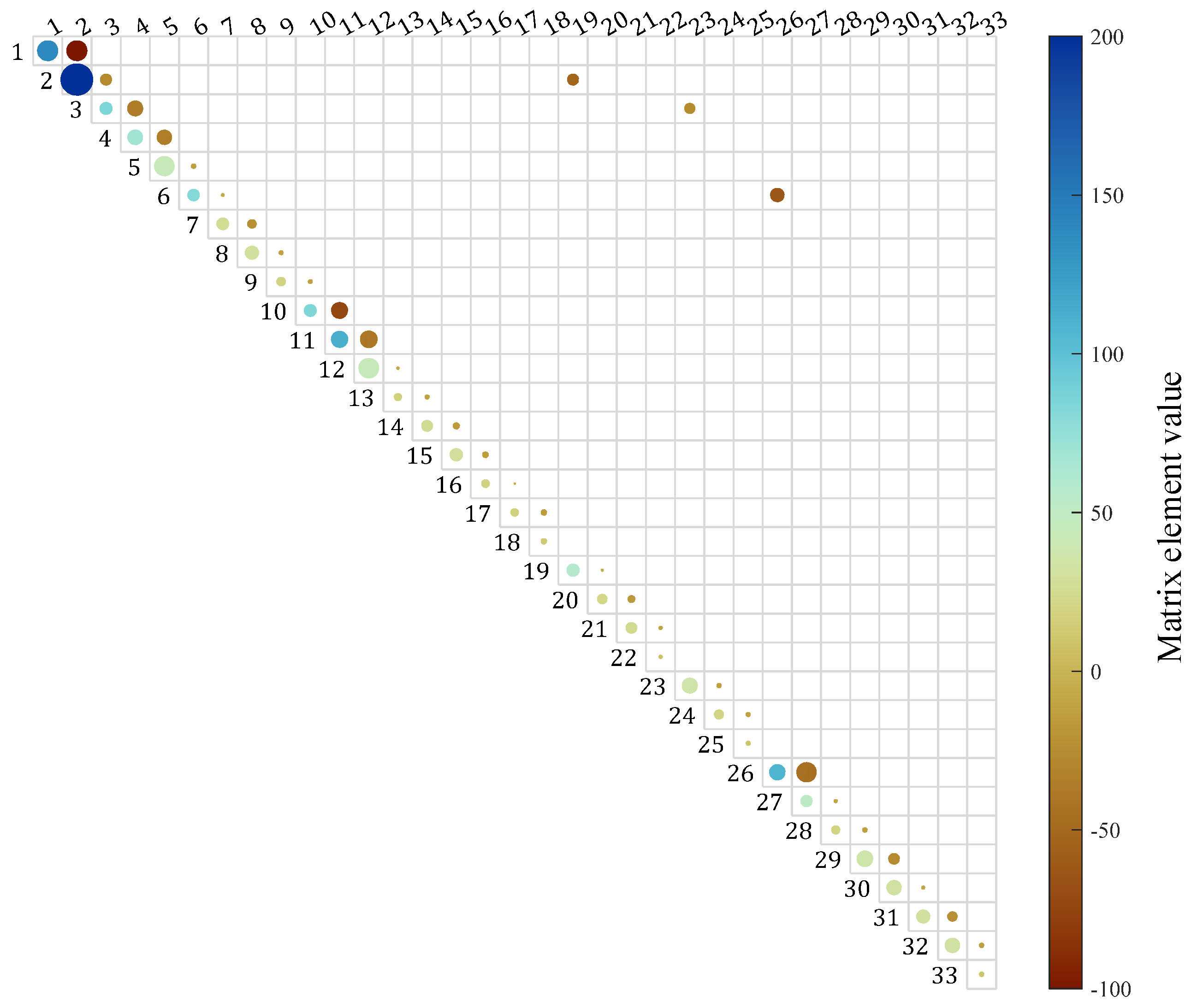
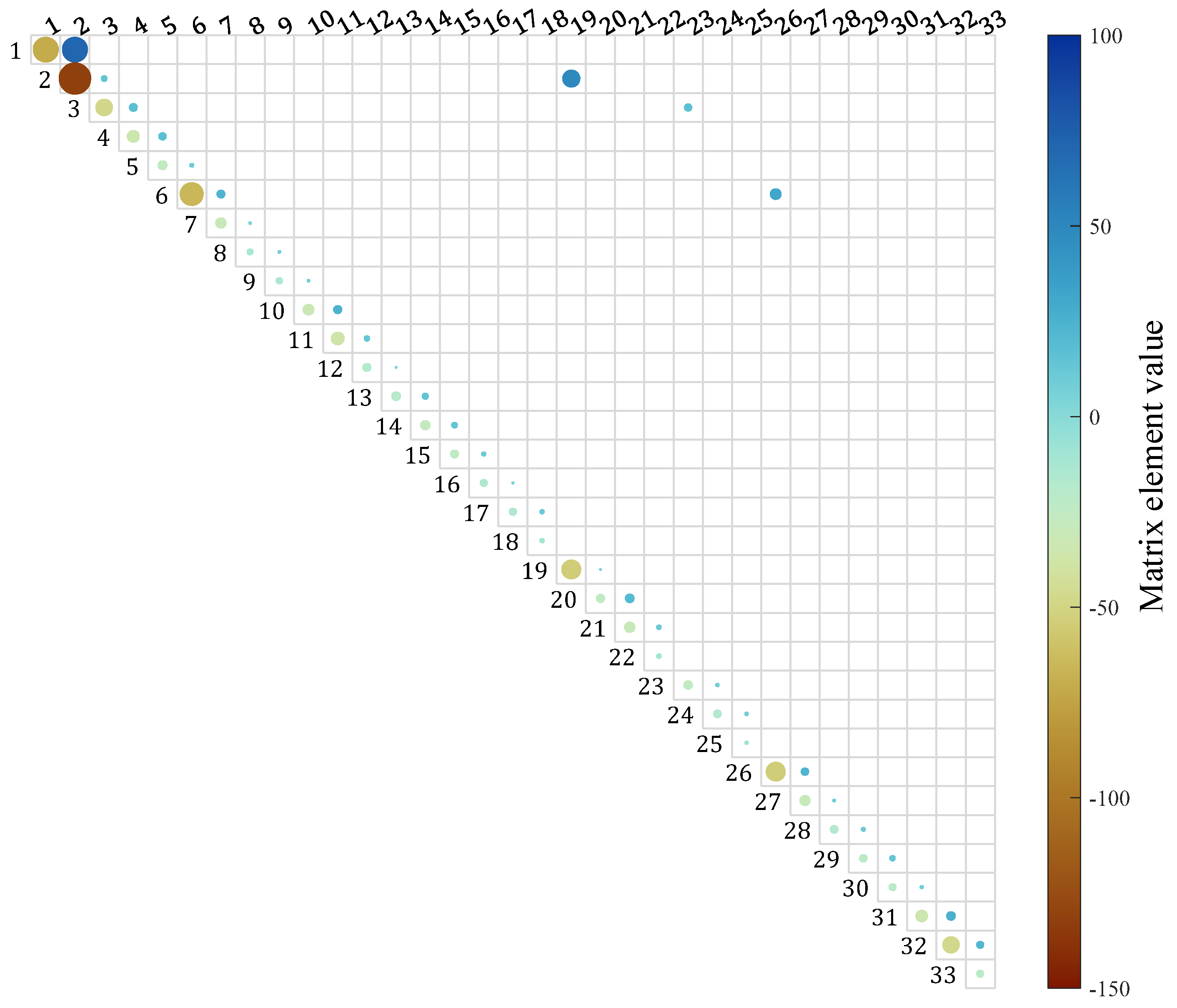
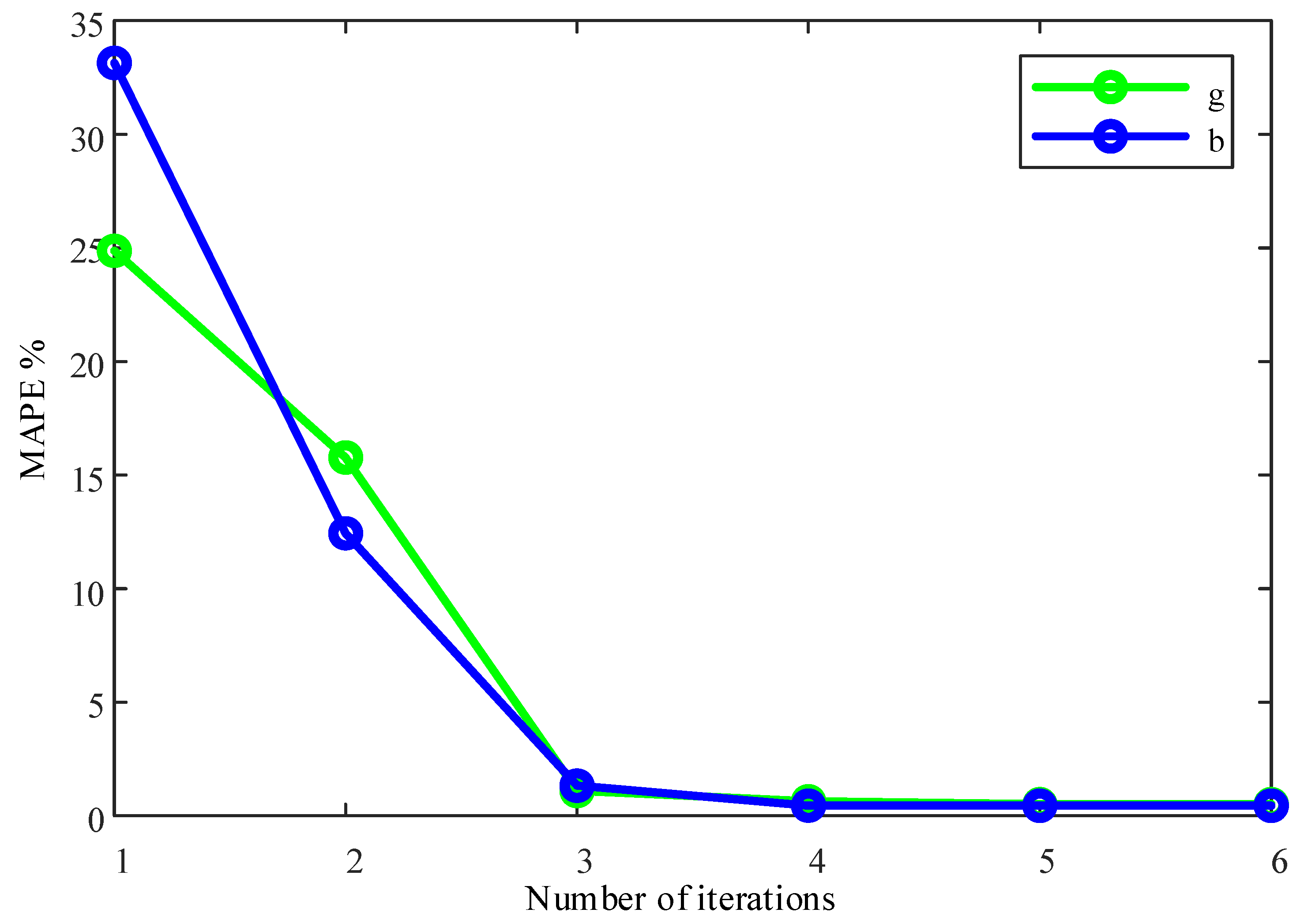
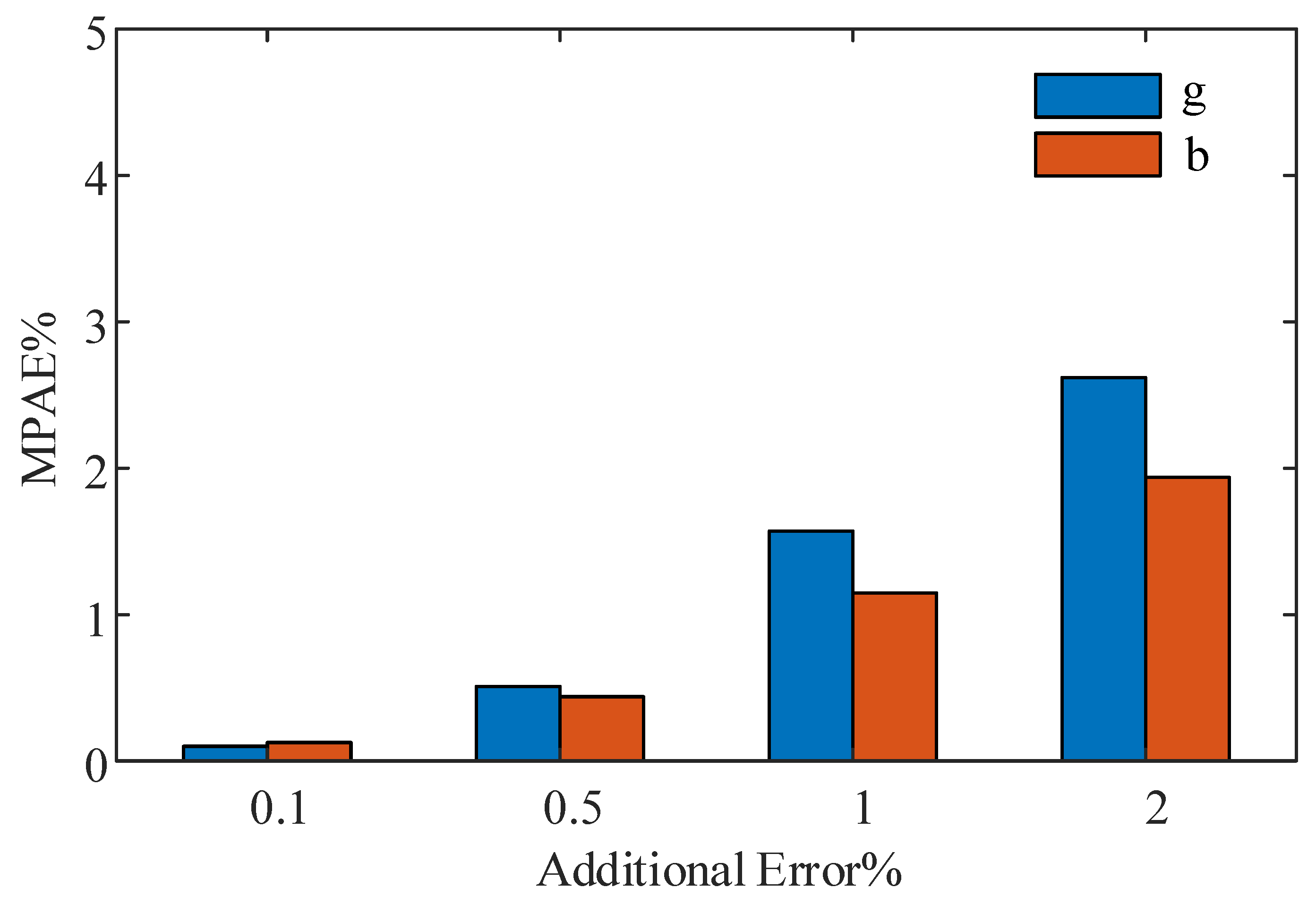
4.2.2. Parameter Identification and Correction

This section validates the effectiveness of parameter correction using the IEEE 33-bus standard test case. The topology of the IEEE 33-bus distribution network is depicted in Figure 6. The system’s nominal voltage is 12.66 kV, and the apparent power base is 10 MVA. Detailed line parameters can be viewed in Appendix A. The network comprises thirty-two connected branches (solid lines) and five unconnected branches (dashed lines). Since topologies constructed from CIM files may contain errors, in this simulation case, the five dashed lines in Figure 6 are assumed to be erroneous branches resulting from the topology construction.

Based on the precision of the medium-voltage distribution network measurement devices, the absolute errors p, q, and v are typically within 0.01%. To evaluate the algorithm’s performance under poor measurement conditions, a 0.5% error was added to the p and q, while a 0.01% error was maintained for the voltage data due to its relative stability.

The active power load curves for each bus over 24 h are shown in Figure 7. Using interpolation, 480 measurement data samples were generated, and the corresponding voltages were calculated to construct the PQV dataset. The power load curves of Bus 15 are shown in Figure 8. Appendix B lists several power load curves.

Based on the known topology (including five erroneous lines), the topology and line impedance parameters of the distribution network were identified and corrected using bus voltage and injected power information. Figure 9, Figure 10, Figure 11 and Figure 12 show the comparison between the obtained line parameters and the actual line parameters. Appendix C shows the heat map of the admittance matrix without reducing noise, given the absence of known topology input.

In the first iteration of the initial identification and correction process, all erroneous lines were effectively identified and subsequently updated to the correct topology by reducing noise. The results indicate that the proposed method can effectively identify and correct erroneous topologies in the distribution network and accurately estimate line parameters. This process not only validates the effectiveness and reliability of the method but also provides reliable data support for subsequent detailed identification and correction.

The average error of the conductance g obtained from the basic discrimination correction is 24.87%, and the average error of the conductance b is 33.14%. The results of the basic discrimination correction are used as the initial values of the fine discrimination correction, and after 10 iterations of the fine discrimination correction, the average error of the conductance g is obtained to be 0.51%, and the average error of the conductance b is obtained to be 0.44%. The comparison between the true values and the fine discrimination correction values is shown in Figure 10.

Figure 11 and Figure 12 present the heat maps of the elements in the admittance matrix after fine correction, visually depicting the magnitude and distribution of each element. The color gradient ranges from blue to brown, representing values from high to low, respectively. The color intensity allows for the quick identification of significant numerical features within the matrix. This visualization method not only effectively displays the distribution characteristics of the admittance matrix but also provides robust support for the parameter correction and identification process, further validating the efficacy of the adopted method in enhancing model accuracy and stability.

To better observe the parameter identification process during correction, Figure 13 illustrates the variation in the mean absolute percentage error (MAPE) of the line parameters g and b throughout the iterations. As indicated by the data in the Figure 13, a total of six iterations were performed. The results clearly demonstrate a trend of progressively decreasing errors with each iteration, further substantiating the effectiveness and reliability of the correction method. This finding not only elucidates the incremental improvements achieved during the parameter correction process but also underscores the significant potential of this method in enhancing model accuracy and stability.

In order to test the effect of different PQ noises on the accuracy of parameter identification correction, this paper analyzes the identification correction of line parameters under additional different noises. Figure 14 reflects the effect of additional errors on active and reactive power on the accuracy of parameter identification correction. From the figure, it can be seen that the errors of line parameters g and b increase with the increase in PQ additional noise, but the overall error of the identification and correction results of this method is small and stable.

5. Conclusions

To address the challenges of constructing distribution network topology models and identifying line parameters without PMU data, this paper proposes a technique based on the Common Information Model (CIM) and measured power-voltage data. Initially, the topology model is constructed using CIM/XML files, and line parameters are preliminarily calculated based on the type and length of AC lines. Subsequently, a regression model is established, based on the constructed topology model and the power flow equations of the distribution network in polar coordinates, to calculate the line admittance parameters obtained from basic identification correction. Finally, a refined parameter identification correction model is established using an improved Newton–Raphson method, iterating through the calculation of the Jacobian matrix until convergence.

The feasibility and accuracy of the proposed method were validated through simulations on the IEEE 33-bus standard test case and an actual case from the Southern Power Grid. The results visually demonstrate that the line parameters obtained through topology model construction and parameter identification correction possess high accuracy, and the method shows robustness under different noise conditions. Compared with other methods, this approach ensures the accuracy of the topology model by leveraging the CIM model, thus enhancing the efficiency and precision of parameter identification correction. The identification and correction results provide effective data support for distribution network analysis and optimization. However, this method has certain limitations when applied to distribution networks with significant data gaps, and its applicability to unbalanced distribution networks requires further investigation. Future research should address these limitations by exploring real-time parameter identification and correction techniques and delve deeper into areas such as fault detection, load forecasting, and power quality analysis.

References

1. Liu, D. Planning Strategy of New Energy System for Power Distribution Network Considering Uncertainty of Source and Load. Guangdong Power 2023, 36, 77–83. [Google Scholar]
2. Zhu, Y.; Yao, R.; Wang, L.; Bai, H.; Li, W.; Du, W.; Xu, M. Sensitivity Analysis Method for Resonant Frequency of Power Grids Based on Singular Value Decomposition. South. Power Syst. Technol. 2024, 1–8. [Google Scholar]
3. Zhang, Y.; Hu, Y.; Wang, D. Automatic Modeling Method of Distribution Network Topology Based on Power Line Communication. Electr. Autom. 2022, 44, 61–62, 66. [Google Scholar]
4. Zhou, L. Research on Self-Healing Technology of Active Distribution Network; Southeast University: Nanjing, China, 2017. [Google Scholar]
5. Li, B.; Sun, M.; Chen, X.; Li, B.; Ji, X.; Xiao, F. Line Parameter Identification Method for Multi-ring Medium-voltage Distribution Network Based on Phaseless Measurement. Autom. Electr. Power Syst. 2023, 47, 22–30. [Google Scholar]
6. Sun, K.; Wang, D.; Ge, X.; Wang, W.; Sun, W. Topoloqical Evolution Model of Power System Based on Positioning Probability and Attenuation Mechanism. Proc. CSU-EPSA 2021, 33, 22–28. [Google Scholar]
7. Ma, D.; Shen, C.; Chen, Y.; Li, D. Feasibility Study on the Convergence Criterion of Power Flow Calculation Based on Deep Learning. South. Power Syst. Technol. 2020, 14, 46–54. [Google Scholar]
8. Kusic, G.L.; Garrison, D.L. Measurement of transmission line parameters from SCADA data. In Proceedings of the IEEE PES Power Systems Conference & Exposition, New York, NY, USA, 10–13 October 2004; Volume 1, pp. 440–445. [Google Scholar]
9. Li, H.; Weng, Y.; Vittal, V.; Blasch, E. Distribution Grid Topology and Parameter Estimation Using Deep-Shallow Neural Network with Physical Consistency. IEEE Trans. Smart Grid 2024, 15, 655–666. [Google Scholar] [CrossRef]
10. Dutta, R.; Patel, V.S.; Chakrabarti, S.; Sharma, A.; Das, R.K.; Mondal, S. Parameter Estimation of Distribution Lines Using SCADA Measurements. IEEE Trans. Instrum. Meas. 2021, 70, 1–11. [Google Scholar] [CrossRef]
11. Shah, P.; Zhao, X. Network Identification Using μ-PMU and Smart Meter Measurements. IEEE Trans. Ind. Inform. 2022, 18, 7572–7586. [Google Scholar] [CrossRef]
12. Guo, Y.; Yuan, Y.; Wang, Z. Distribution Grid Modeling Using Smart Meter Data. IEEE Trans. Power Syst. 2022, 37, 1995–2004. [Google Scholar] [CrossRef]
13. Yu, J.; Weng, Y.; Rajagopal, R. PaToPaEM: A Data-Driven Parameter and Topology Joint Estimation Framework for Time-Varying System in Distribution Grids. IEEE Trans. Power Syst. 2019, 34, 1682–1692. [Google Scholar] [CrossRef]
14. Park, S.; Deka, D.; Backhaus, S.; Chertkov, M. Learning With End-Users in Distribution Grids: Topology and Parameter Estimation. IEEE Trans. Control Netw. Syst. 2020, 7, 1428–1440. [Google Scholar] [CrossRef]
15. Luan, W.; Peng, J.; Maras, M.; Lo, J.; Harapnuk, B. Smart Meter Data Analytics for Distribution Network Connectivity Verification. IEEE Trans. Smart Grid 2015, 6, 1964–1971. [Google Scholar] [CrossRef]
16. Pappu, S.J.; Bhatt, N.; Pasumarthy, R.; Rajeswaran, A. Identifying Topology of Low Voltage Distribution Networks Based on Smart Meter Data. IEEE Trans. Smart Grid 2018, 9, 5113–5122. [Google Scholar] [CrossRef]
17. Zhao, J.; Li, L.; Xu, Z.; Wang, X.; Wang, H.; Shao, X. Full-Scale Distribution System Topology Identification Using Markov Random Field. IEEE Trans. Smart Grid 2020, 11, 4714–4726. [Google Scholar] [CrossRef]
18. Tian, Z.; Wu, W.; Zhang, B. A Mixed Integer Quadratic Programming Model for Topology Identification in Distribution Network. IEEE Trans. Power Syst. 2016, 31, 823–824. [Google Scholar] [CrossRef]
19. Zhang, S.; Liu, G. Introduction to IEC61970 standard series. Autom. Electr. Power Syst. 2002, 14, 1–6. [Google Scholar]
20. Chen, G.; Zhang, Z.; Hong, X.; Li, C. Modeling Method for Digital Twin of Distribution Automation Terminal Based on lEC 61968. Power System Technol. 2024, 1–9. [Google Scholar] [CrossRef]
21. Cai, W.; Fang, W.; Zhu, W.; Liu, P.; Xia, W. Power system graph model data fusion technology based on CIM/SVG. J. Shenyang Univ. Technol. 2023, 45, 656–660. [Google Scholar]
22. Xu, Y.; Ma, W.; Zhao, L.; Weng, Y.; Zhen, H.; Shi, J.; Zhai, H.; He, X. Multi-Granularity Power Flow Calculation Data Construction Method Based on ClM. South. Power Grid Technol. 2022, 16, 40–47. [Google Scholar]
23. Wang, X.; Zhang, J.; Du, X.; He, X.; Zhang, W.; Zhao, B.; Liu, Q. Optimal Allocation of Energy Storage in Distribution Networks Based on Electric Common Information Model. South. Power Syst. Technol. 2024, 18, 112–123. [Google Scholar] [CrossRef]
24. Zhou, L.; Wang, T. Research on CIM model based on IEC61970. Sci. Technol. Inf. 2013, 89+93. [Google Scholar]
25. Ao, X.; Wang, C.; Zhu, W.; Xiao, Y. Derivation and Comparison of Two Versions of Linear Power Flow Method for Distribution Networks. Power Syst. Technol. 2017, 41, 4004–4013. [Google Scholar]
26. Zhang, J.; Wang, Y.; Weng, Y.; Zhang, N. Topology identification and line parameter estimation for non-PMU distribution network: A numerical method. IEEE Trans. Smart Grid 2020, 11, 4440–4453. [Google Scholar] [CrossRef]
27. Chen, J.; Zhang, X. Decompositions and Generalized Inverses of Matrices. Univ. Math. 2019, 36, 57–66. [Google Scholar]
Figure 1. Flowchart for topology construction.
Energies 17 03611 g001
Figure 2. Schematic diagram of the topology reduction process.
Energies 17 03611 g002
Figure 3. Application of least squares to parameter identification.
Energies 17 03611 g003
Figure 4. Overall flowchart of the parameter correction algorithm.
Energies 17 03611 g004
Figure 5. Topology node connection diagram. (a) Before topology reduction; (b) After topology reduction.
Energies 17 03611 g005
Figure 6. IEEE-33 bus system topology connection diagram.
Energies 17 03611 g006
Figure 7. 24 h active power load curves of each bus.
Energies 17 03611 g007
Figure 8. Active power and reactive power of bus 15 in 24 h.
Energies 17 03611 g008
Figure 9. Basic corrected g and b values vs. actual value.
Energies 17 03611 g009
Figure 10. Fine corrected g and b values vs. actual values.
Energies 17 03611 g010
Figure 11. Fine-corrected G-matrix.
Energies 17 03611 g011
Figure 12. Fine-corrected B-matrix.
Energies 17 03611 g012
Figure 13. Variation in the MAPE of g and b throughout the iterations.
Energies 17 03611 g013
Figure 14. Mean errors of g and b for different PQ noises.
Energies 17 03611 g014