Abstract
With the development of the power distribution Internet of Things (IoT), the escalating power demand of data centers (DCs) poses a formidable challenge to the operation of distribution networks (DNs). To address this, the present study considers the operational flexibility of DCs and its impact on DNs and constructs a collaborative planning framework of DCs, renewable energy sources (RESs), and DNs. This framework employs the interval optimization method to mitigate uncertainties associated with RES output, wholesale market prices, carbon emission factors, power demand, and workloads, and the collaborative planning model is transformed into an interval optimization problem (IOP). On this basis, a novel hybrid solution method is developed to solve the IOP, where an interval order relation and interval possibility method are employed to transform the IOP into a deterministic optimization problem, and an improved integrated particle swarm optimization algorithm and gravitational search algorithm (IIPSOA-GSA) is presented to solve it. Finally, the proposed planning framework and solution algorithm are directly integrated into an actual integrated system with a distribution network and DC to verify the effectiveness of the proposed method.
1. Introduction
In recent years, with the burgeoning development of the power distribution Internet of Things (IoT), Data centers (DCs), as pivotal entities for large-scale data storage and computation, are projected to expand in scale continuously. It is estimated that the energy consumption of data centers already comprises approximately 2% of global electricity usage, with an anticipated annual growth rate of 15% to 20% [1]. Consequently, if the DC load is supplied primarily by China’s current fossil-fuel-dominated power grid structure, which comprises roughly 70% of energy generation, this could adversely affect the security and economic efficiency of power system operations while contributing to substantial carbon emissions. This, in turn, could obstruct the achievement of the carbon neutrality goal [2].
Acknowledging the heightened global concern over climate change, China has committed to achieving “carbon peaking” by 2030 and aspires to attain “carbon neutrality” by 2060 [3]. In pursuit of these ambitious carbon emission reduction targets within distribution networks (DNs), particularly amidst the proliferation of large-scale data center (DC) integration, incorporating renewable energy sources (RES) such as wind turbines and photovoltaic systems into DNs is recognized as a pivotal strategy. Nevertheless, RESs within DNs, exemplified by solar and wind power, are inherently volatile and unstable due to geographical location, weather conditions, time of day, and other factors, posing significant challenges in scheduling operations [4].
To promote the consumption of RESs and realize carbon emissions reduction, three key measures can be implemented. Firstly, harnessing the operational flexibility of geographically dispersed data centers (DCs) can significantly enhance the absorption of RESs, thereby aligning with carbon reduction targets. Distinct from other major energy consumers, DCs, reliant on information networks, possess temporal and spatial load regulation capabilities facilitated by the scheduling of delay-tolerant workloads (DWs) and real-time workloads (RWs) [5]. Furthermore, given the presence of cooling systems in DCs, the thermal inertia inherent in DC buildings can be exploited to further enhance temporal load regulation potentials. By integrating these three avenues for DC load regulation, it becomes feasible to consume entirely zero-emission RES-generated electricity, ultimately contributing to a reduction in carbon emissions.
Secondly, implementing source–network–load collaborative optimization from a long-term perspective is crucial. The effectiveness of leveraging DCs’ flexibility, encompassing spatiotemporal workload scheduling and thermal inertia processes, in promoting RES consumption and mitigating carbon emissions within distribution networks (DNs) is fundamentally contingent upon the strategic location and capacity of RES sources, DCs, and distribution lines.
Thirdly, the adoption of advanced uncertainty modeling methods is imperative for the collaborative optimization of DNs, DCs, and RESs under uncertain conditions. Two primary approaches exist for managing RES-related uncertainties: robust optimization (RO) and stochastic optimization (SO). However, RO, grounded in worst-case analysis, often results in overly conservative solutions. Conversely, SO necessitates prior knowledge of the probability distribution of uncertain variables to generate scenarios, which can be challenging when the distribution of uncertain parameters remains elusive. Consequently, the development of innovative uncertainty modeling techniques is paramount.
Based on the above analysis, it is urgent to exploit a collaborative planning framework of DNs, DCs, and RESs in an uncertain environment to achieve the carbon reduction target, wherein the operational flexibility of DCs would be fully considered. The key research questions addressed in this context are as follows:
- ▪
- How can a collaborative optimization of DCs, RESs, and DNs be developed from a long-term planning perspective to promote carbon reduction?
- ▪
- How can multidimensional uncertain factors be modeled in a collaborative planning setting?
- ▪
- How can the mathematical model with interval variables be solved efficiently?
2. Literature Review
Growing research effort has been expended on the energy management of DCs in the last several years.
In order to deal with the high energy consumption problems of DCs, existing research has explored the development of energy-saving technology from the DC-equipment level. The authors of [6] proposed incorporating a hybrid air/liquid-cooled server in the DC to improve the effectiveness of cooling and waste-heat recovery. Reference [7] presented a dynamic voltage frequency scaling technique for physical servers to reduce power consumption. In [8], a dynamic virtual machine consolidation technique was developed for a DC to minimize energy consumption. Reference [9] proposed a real-time optimization of a liquid-cooled DC based on cold plates to save energy. The work of [10] presented a novel data center free radiating system driven by waste heat and wind energy to reduce cooling consumption.
Despite the notable benefits associated with DC energy savings outlined in the aforementioned studies, these efforts have primarily centered around DC self-scheduling, overlooking the potential flexibility of DCs within the context of DNs. Nevertheless, it is imperative to acknowledge that achieving low-carbon operation in DC-integrated DNs solely through equipment-energy-saving techniques may prove exceedingly challenging due to technological and financial constraints [11]. As mentioned above, DCs could be exploited as a potential flexibility resource in the DNs via the spatio-temporal scheduling of workloads and a building’s thermal inertia process. Specifically, based on the operator’s requirements, the DW could be shifted to low-tariff periods or high-RES-output periods for processing before deadlines; the RW could be dispatched to a low-load DC for processing to improve system economy efficiency and promote renewable energy consumption. In addition, the thermal inertia processes of DC building could be utilized to schedule the cooling power to enhance system performance.
Given this, some studies, starting from the DN level, have developed the flexibility of DCs and facilitated the interaction of DCs and DNs to increase operation efficiency. For instance, Reference [12] proposed a DN dispatch model considering DC flexibility to improve energy efficiency. In [13], a flexible scheduling strategy of workloads is proposed for an internet DC with renewable energy, an electric energy storage device, and a water-cooling system to reduce the operating cost. Reference [14] proposed a coordinative optimization model for demand response among multiple DC operator and system operator. Reference [15] proposes a data center microgrid supply-and-demand scheduling problem to minimize operation costs and wind power curtailment by profoundly exploring the temporal distribution of workloads. Ref. [16] proposed an online algorithm based on the Lyapunov optimization framework developed for the optimal coordination of DCs in a regional cluster to reduce operational costs and save computation, considering the flexibility of the computing workload. Considering the schedules of workloads, Reference [17] proposed a cooperative online schedule framework for local interconnected DCs considering shared energy storage to reduce operation costs and carbon emissions. Reference [18] developed an online job-scheduling scheme for low-carbon DC operation. A coordinated operation framework of DCs and power systems was proposed by [19] to facilitate renewable energy integration. Reference [20] proposed a coordinated optimization model of the operational scheduling of integrated energy systems for DCs according to computing load transfer.
While the aforementioned literature has indeed made significant contributions to energy savings and emission reduction through harnessing the flexibility of DCs, their research endeavors remain limited by two pivotal shortcomings, as noted below.
On the one hand, the majority of existing research endeavors have predominantly explored DC flexibility from an operational standpoint, neglecting the crucial long-term planning perspective. In reality, maximizing the benefits derived from DC flexibility in DNs, such as the spatiotemporal scheduling of workloads and the effective utilization of thermal inertia, is inherently tied to the strategic site selection and optimal capacity allocation of the constituent components. For instance, the location of the DC and the configuration of servers and cooling systems play pivotal roles in determining the DC’s operational flexibility and the resultant enhancement of DN performance [21]. Consequently, to fully realize the potential benefits of DC flexibility, it is imperative for system operators to delve into the optimal integration and configuration of distribution systems with DCs and RESs through a planning approach. While a few studies have begun to address the planning problem associated with DCs [22,23,24,25], their focus remains primarily on the standalone planning of DC configurations, overlooking the imperative need for collaborative planning.
On the other hand, existing investigations concerning DCs and their flexibility have predominantly overlooked the intricate multidimensional uncertainties inherent in the system [6,7,8,9,10,11,12,13,14,16,17,18,19,20,21,22,23]. Alternatively, they have resorted to either stochastic optimization (SO) [21,25] or robust optimization (RO) [15,24]. The intermittent nature of renewable energy sources (RESs) introduces substantial uncertainty in output levels, heavily influenced by meteorological fluctuations. Furthermore, the electric load and workloads accessed by DCs exhibit stochasticity, stemming from the unpredictable behavior of end-users. Moreover, external factors such as electricity prices and emission coefficients from the grid remain uncertain.
In practical applications, if the flexibility of DCs within distribution networks (DNs) is exploited solely from a long-term planning perspective, without accounting for these multifaceted uncertainties, this could lead to overly optimistic projections. Consequently, this may result in an overreliance on external, high-emission electricity sources and underutilization of renewable energy. Additionally, RO, rooted in worst-case analysis, tends to be overly conservative, while SO necessitates prior knowledge of uncertainty variable probability distributions for scenario generation, which can be challenging when such distributions remain unknown.
To harmonize the strengths of both approaches, interval optimization (IO) methodologies have been devised and deployed to address uncertainties. In contrast to SO, IO characterizes uncertainty through interval variables, delineated by their lower and upper bounds derived from a dataset. This approach facilitates implementation within the context of long-term planning, as it simplifies the requirement for detailed probability distributions [26]. IO is designed to minimize the interval of the objective function, avoiding overly conservative decisions [27]. For instance, reference [28] developed an available transfer capability evaluation model based on IO. For the uncertainty caused by household load and photovoltaic systems, an IO method considering integrated demand response and tolerance degree was presented for the household-load-scheduling problem [29]. In light of the uncertainty of demand response and wind power, a coordinated operating strategy of the gas–electric integrated energy system based on IO was investigated to improve overall system operation [30]. Reference [31] proposed a low-carbon economic dispatch model in renewable energy power systems, where the IO was used to manage the uncertainty of wind power output. A comparison of the reviewed literature is summarized in Table 1.

Table 1.
Comparison of the proposed approach with related studies.
Contributions and Paper Organization
This paper establishes a collaborative planning framework of DCs, RESs, and DNs to promote the low-carbon development of DC-integrated DNs. Interval optimization is employed to consider the system’s uncertainties, such as RES output, electricity price, emission factor, power load demand, and workloads, consequently, the planning model is reformulated as an interval optimization problem. Then, to tackle this reformulated problem, an improved integrated particle swarm optimization algorithm and gravitational search algorithm (IIPSOA-GSA) is developed. Finally, to verify the proposed method’s effectiveness, the improved IEEE-33 node distribution network is taken as an example to verify the effectiveness of the proposed planning model and algorithm.
The main contributions of this paper are summarized as follows:
(1) A collaborative planning framework for the integration of DCs, RESs, and DNs is developed to foster the low-carbon evolution of distribution systems. Targeting the efficient integration of DCs and DNs, a collaborative planning model for DCs and DNs is developed. Considering the uncertainties existing in the system, the planning framework is reformulated as an interval optimization problem to co-optimize economic and environmental performances.
(2) Multifaceted uncertain factors associated with DC-integrated DNs are modeled through interval optimization. In contrast to prevailing research, uncertainties pertaining to RES output, electric load demand, workload demand, electricity prices, and emission factors from the external grid are explicitly incorporated. The above uncertainties are represented as interval numbers obtained via the fluctuation in long-term planning. These considerations make our work distinctive and more practical in reality, ultimately resulting in more persuasive planning results.
(3) A novel hybrid solution methodology that combines interval order relation, interval possibility, and the IIPSOA-GSA is proposed to solve the interval optimization. To solve the IO-based collaborative planning model, the interval order relation method (IORM) and interval possibility method (IPM) are leveraged to transform the IO model into a deterministic optimization model, and a hybrid modified gravitational search algorithm and particle swarm optimization algorithm is developed to solve the transformed model efficiently.
The remainder of this paper is structured as follows. Section 3 outlines the model framework. In Section 4, the DC model is elaborated upon. Section 5 presents a collaborative planning model for a DN, RESs, and DCs. Section 6 introduces the solution methodology employed. Section 7 conducted case studies. Section 8 discusses the limitations of the proposed theoretical framework. Finally, Section 9 concludes the paper and elaborates on the extension of this research.
3. Model Framework
3.1. System Structure
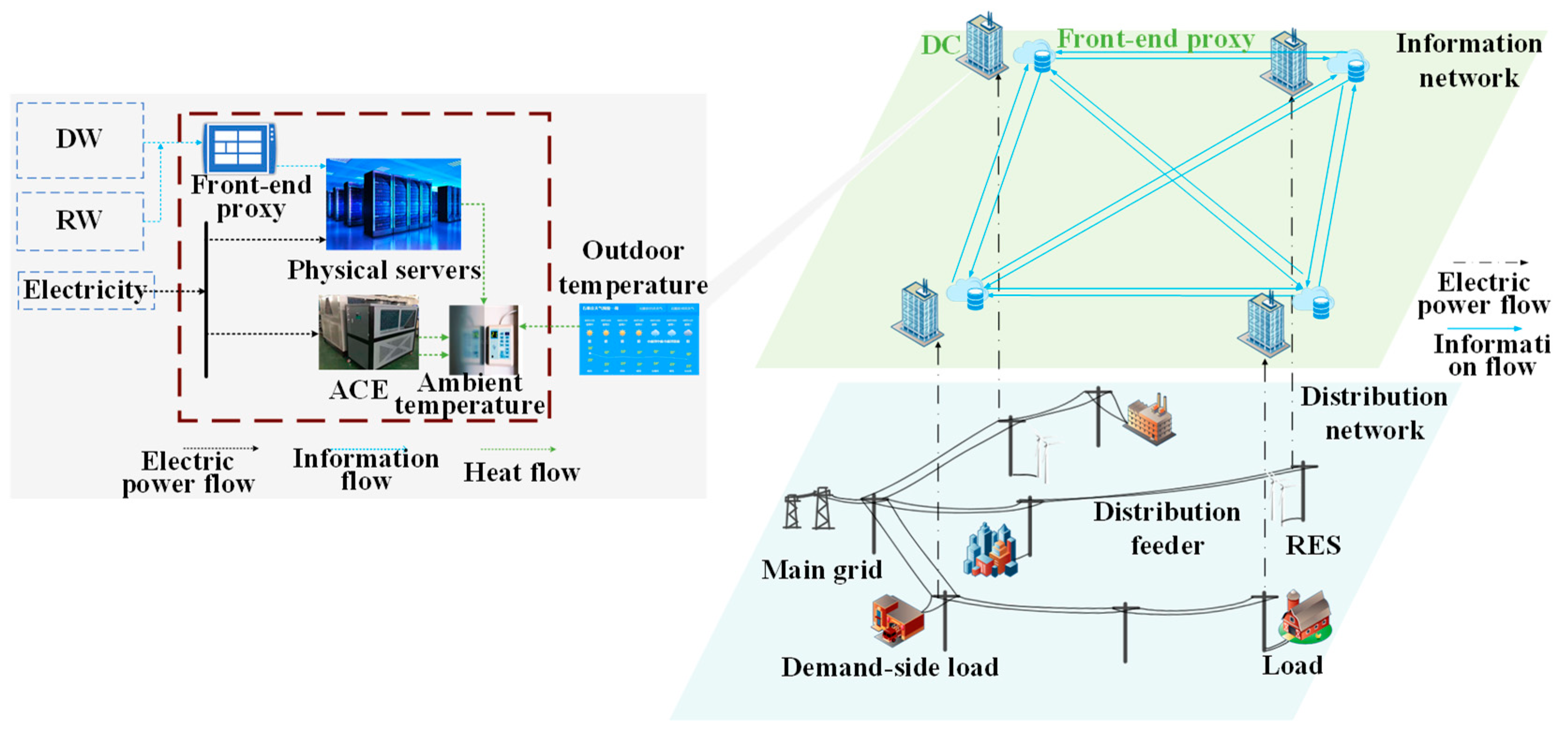
A schematic representation of the typical equipment configuration in a data center is depicted on the left side of Figure 1. Within the DC, the equipment consists of IT, primarily physical servers, and supplementary devices. Considering the strict temperature constraints of physical servers, the air-conditioning equipment (ACE) must be equipped in the DC. In addition, a front proxy in the DC is responsible for collecting and distributing workloads.

Figure 1.
Architecture of DC–distribution network integrated system.
Workloads can broadly be classified into two categories: delayable workloads (DWs) and real-time workloads (RWs) [32]. DWs encompass tasks with a predefined volume to be processed within a specified time frame yet offering flexibility in the processing timeline. Conversely, RWs involve processing requests with strict timing constraints, allowing for their transfer between geographically dispersed DC regions.
3.2. Model Framework
In the context of the profound development of the power distribution IoT, Power grid company are increasingly being encouraged to establish dedicated private DC systems, specifically ones tailored to facilitate calculations for DNs [33] and leverage high-performance-computing capabilities to support their operations [23]. As a result, the DC and DN operate as an integrated unit, where DCs are utilized for the analysis of DN data, while the DN provides reliable power to the DCs. Consequently, it is postulated that the distribution network operator (DSO) performs both investment and operation of DCs, RESs, and the DN.
The architecture of this integrated system is depicted in the right-hand section of Figure 1. It is evident that the system encompasses both an information network and the DN. The information network comprises geographically dispersed DCs, whereas the DN primarily consists of distribution feeders and RESs. The DN interfaces with the primary grid through a distribution substation, supplying electricity to demand-side users within the DN, including DCs, via external market electricity acquisitions and distributed power generation.
In this context, the operator is charged with devising an optimal system configuration scheme to minimize economic costs. However, the decision-making process is intricately linked to multidimensional uncertainties. To tackle these uncertainties, this study employs interval optimization, where uncertain variables are represented by compiling predicted confidence intervals. Each interval is defined by the upper and lower bounds of uncertain parameters based on forecasting values and statistical data spanning a year.
In conclusion, the collaborative planning of the DN, RES, and DC is formulated as an interval optimization model, which aims to improve economic and environmental performance. However, the interval representation poses challenges in solving the model. To address this, we initially leverage the IORM and IPM to convert the IOP into a deterministic model and develop an IIPSOA-GSA approach to solve the proposed IO problem.
4. DC Modeling
4.1. Information Domain
4.1.1. Delay-Tolerant Workloads (DW)
Considering the nature of DW requirements, the DW characteristic is represented as follows:
Equation (1) delineates the proportion of DW to the total workloads, where the subscripts t and d represent the index of the time period and the DC, respectively, and the superscript DW0 represents the index of the initial DW demand. Equation (2) ensures the actual processed DW is related to the DWs that have arrived, the DW transferred to another time period, and the DW transferred to this time period, where the subscript tt’ represents the time period from t to t’, and the superscripts DW and DWT represent the index of the DW demand and transferred DW demand. T is the total operating period. Equation (3) ensures that the transferred DWs cannot exceed the DWs that have arrived. Equation (4) constrains the total transferred DWs so that they cannot exceed the DWs that arrived at a given time.
4.1.2. Real-Time Workloads (RWs)
For the scheduling control of RW, the relevant constraints are expressed as follows:
Equation (5) represents the proportion of RWs to the total workloads, and the superscript RW0 represents the index of the initial RW demand. Equation (6) states that the actual processed RW is the RWs that have arrived minus the RW transferred to other distributed DCs and adds the RW transferred to that DC, where the subscript dd’ represents the DW from the DC d to d’, and the superscript RW represents the index of the DW demand.
Based on Equations (1)–(6), considering the spatial and temporal distribution of workloads, the total workload that DCs need to process is determined by (7).
4.1.3. Quality of Service Requirement
Indeed, when handling workloads, one must account for inherent transmission and queuing latencies. To ensure that DCs maintain an acceptable quality of service (QoS), it is imperative that the queues and handling latencies remain below the workloads’ maximum permissible delay threshold. Therefore, based on M/M/1 queue theory, the QoS of workloads can be determined as follows [34]:
Equation (8) calculates the queue waiting time based on the M/M/1 queue theory, where the superscripts Queue and ser-on represent the index of the queue time delay and power for servers. Equation (9) indicates that the workload’s processing time is inversely proportional to the server processing speed, where the superscript Handle represents the handle time delay. Equation (10) stipulates that the total workload time delay cannot exceed the maximum allowable delay.
4.2. Physical Domain
4.2.1. Thermodynamic Process
As already mentioned, the ACE is integrated within the DC to ensure that the ambient environmental temperature is consistently maintained within a safe operational range, thereby guaranteeing stable operation. In this context, by considering the operational interval of the ambient environmental temperature, the ACE can be flexibly dispatched during actual operation to provide support for the DN and improve its own performance. This attribute is colloquially referred to as thermal inertia. This subsection presents a detailed thermodynamic model of the DC, as outlined in (11)–(15).
As detailed in Equation (11), a thermal balance is established among the ambient environmental temperature, the heating power emanating from the servers, the cooling power supplied by the ACE, and the outdoor temperature based on the principle of building thermal equilibrium, where H represents the heat generated by the ambient environmental, servers, and ACE, while V stands for the DC space volume. Equation (12) characterizes the heat transfer occurring through the external walls of the DC, which is quantified by multiplying the pertinent coefficient by the temperature differential between the external walls and the interior of the DC. The heat emanating from the operational physical servers can be computed as illustrated in Equation (13). Equation (14) imposes a constraint on the ambient environmental temperature to ensure the stable operation of the data center (DC). Additionally, Equation (15) defines the permissible range for the temperature variation rate within the DC structure.
4.2.2. Power Consumption Characteristics
The total power consumption of the DC during operation primarily includes two parts, namely, IT equipment and ACE, as shown in (16).
The total power consumption of IT equipment is predominantly determined by the number of operating servers, the fixed power consumption of an individual physical server, the peak power consumption of a single physical server, and the prevailing data load during the current timeframe, as depicted in Equation (17), where the superscripts Serv-p and Serv-s represent the index of the peak and silent power. For the sake of simplicity, this study assumes that all servers within the DC are identical and the workload at any particular instant is evenly distributed across all active servers. Moreover, the total number of servers that turned on within the DC should not surpass the installed capacity, as stipulated in Equation (18). Furthermore, Equation (19) limits the CPU utilization rates of the physical servers.
The operational characteristics of the ACE are defined by Equations (20) and (21). The cooling power generated by the ACE is calculated based on its power consumption and energy efficiency coefficient, as expressed in Equation (20). Additionally, Equation (21) ensures that the ACE power consumption does not exceed its installation capacity constraints, where the superscript ACE-R indicates the rated power of the ACE.
5. A Collaborative Planning Model for the DN and DC Based on Interval Optimization
5.1. Objective Function
The suggested interval-based collaborative planning framework aims to reduce financial expenditures, encompassing both the annualized costs of capital investment and the expenses incurred from operations, as delineated below.
The investment expenditure consists of the costs associated with RESs, DNs, and the DC’s equipment installation, represented as (23), where the subscripts ij, m, and r represent the index of the distribution lines, the type of distribution lines, and the RES, while the superscripts TF-add, Line, and RES-rated represent the index of the expansion capacity of the distribution transformer, the distribution lines, and the rated power of the RES.
The operational expenditure includes electricity expenditure, RES curtailment expenditure, and the loss cost about DC flexibility:
Equation (25) represents the electricity purchase cost, computed by multiplying the prevailing market price by the quantity of electricity procured. The penalty cost associated with the curtailment of RES, as detailed in Equation (26), is formulated based on the penalty factor and the volume of RES curtailed, where the superscript ‘wat’ designates the index for the wasted RES quantity. Equation (27) encapsulates the costs incurred by the DC’s participation in demand response programs. Furthermore, in practical scenarios where fossil-fuel-based energy sources contribute significantly to the generation mix within a DN, the construction of energy-intensive DCs would result in substantial carbon emissions. Consequently, this study incorporates the carbon emissions cost, as outlined in Equation (28).
5.2. Constraints Conditions
5.2.1. Planning Stage
During the planning phase, it is crucial to incorporate capital costs and land area constraints, thereby necessitating the imposition of corresponding limitations on the construction of diverse components. Equations (29)–(32) explicitly define these planning-related constraints.
5.2.2. Operation Stage
- (1)
- RES
The power production from RES units is constrained by the planning capacity and the load factor, signifying the impact of meteorological conditions [35]:
- (2)
- DN
To maintain the voltage quality within the DN in accordance with established standards, it is imperative to impose constraints on voltage fluctuations, as stipulated in Equation (35). The balance of active and reactive power flow at each node within the DN is represented by Constraints (36) and (37), where the subscripts i and j signify the indices of the buses in the DN. Constraints (38) and (39) delineate the voltage drop experienced across each distribution feeder within the DN. Moreover, Constraint (40) specifies that the power transmitted through each distribution feeder must remain within permissible limits. Finally, the power flowing from the distribution transformer, subject to the transformer’s installed capacity, must adhere to the constraints outlined in Equation (41).
5.2.3. Uncertain Variables
As previously stated, the decision-making process concerning collaborative planning is intricately linked to various uncertainties, primarily stemming from RES outputs, electricity prices, carbon emission factors, electrical load demands, and workloads. To address these uncertainties within our proposed planning framework, an interval-based methodology is employed, as exemplified in (42)–(46), where the superscripts − and + represent the lower and upper bounds of the interval variables.
6. Solution Algorithm
The general formulation of the collaborative planning is presented as follows:
In this study, X is a planning variable vector; Y is an operational variable vector; U is an uncertain variable vector; and is the parameter vector of the constraints.
6.1. Deterministic Transformation
Considering the interval variables in the model l, the solution process becomes more complex. In this paper, the objective function and constraints are transformed by introducing an IORM and IPM so that the proposed optimization problem with interval parameters can be converted into a deterministic model. The specific process is presented as follows.
In the IO model, for the objective function , the fluctuation due to interval variables at the decision variables can be represented by interval numbers . can be calculated using (51) and (52).
To objectively evaluate the value of the interval objective and identify the best solution, the interval objective function is addressed by the IORM, which equivalently transforms them into a deterministic objective consisting of the midpoint and the deviation value [27], as shown in (53)–(55), where denotes the optimization objectives for the proposed model.
In actual implementation, considering the different preferences for investment risks and benefits for the decision makers, this study integrates and by using the linear weighted summation method, finally resulting in the following deterministic objective function:
Similarly, for each interval constraint, the fluctuation caused by uncertain variables at the decision variables can be represented by interval numbers. The interval possibility method is used to address the interval-formed constraints. In the interval possibility method, the possibility function is used to assess whether the interval meets the specified constraint, which would be more fit to transform the interval-form constraints [29]. The constraints can be transformed into the following formulation based on the interval possibility method.
where denotes the possibility limit for constraint i, and its value defines the feasible region of the optimization problem. That is, a larger indicates that the operator would be stricter with the constraint.
By following the aforementioned steps, the IO model proposed in this study was converted into a deterministic model.
6.2. Improved Integrated PSOGSA Algorithms
6.2.1. Traditional PSO and GSA
Particle swarm optimization (PSO) is a population-based algorithm inspired by the collective behavior of flocks of birds [36]. In PSO, particles represent potential solutions to the optimization problem. The velocity of these particles serves a crucial role. It determines how the particles move through the search space in their quest for the optimal solution. The velocity component in PSO is inspired by the swarming behavior observed in nature, where r particles adjust their movement based on their own experience (personal best) and the experience of their neighbors (global best). By updating their velocity, particles are able to explore new areas of the search space while also exploiting known good regions, balancing exploration and exploitation. The formulae for updating the velocity and position of a particle in the ith dimension is as follows:
where represent the inertia weight, and represent learning constants, and represent two random numbers.
The gravitational search algorithm (GSA), rooted in Newton’s law of universal gravitation and mass interactions [37], formulates an optimization framework where a collection of masses, conceptualized as potential solutions, interact based on Newtonian gravity and motion principles. Within this context, the search domain is traversed by these masses as they seek to optimize a given problem with N masses, defined as follows:
In the m-th iteration, the gravitational force on mass i from mass j in a dimension d is determined by (61)–(63).
where and represent the passive gravitational mass related to mass i and the active gravitational mass related to mass j, while denotes the gravity constant, shown in (62). represents the Euclidean distance between mass i and mass j, calculated via (63):
Therefore, the total gravitational force acting on mass i is determined as follows:
Then, based on the law of motion, the acceleration of mass i is calculated using (65).
Based on the acceleration, the velocity and position of mass i are given as follows:
Notably, a greater mass indicates a better solution, which implies an object could induce stronger attraction and move at a slower pace. Given the gravitational and inertial mass equivalence, the gravitational and inertial masses are updated using (68)–(70).
6.2.2. IIPSOA-GSA
The above description shows that the PSO algorithm faces a dilemma between global exploration and local exploitation, making it tend to converge prematurely to the local optimum. To address the above challenge, by integrating the preponderance of the GSA, an IIPSOA-GSA is proposed to solve the collaborative planning problem, which could achieve an equilibrium between exploration and exploitation.
- (1)
- Improved particle-updating scheme
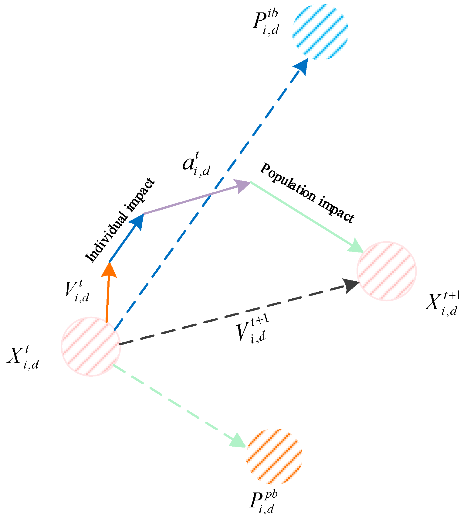
In the IIPSOA-GSA, by combining the acceleration of GSA into the local search part of the PSO algorithm and taking into account the adaptive coefficient, the position and velocity of a particle based on the improved particle-updating scheme are defined in (71) and (72):
where and denote the adaptive coefficients for the particle and population, respectively.
It is noteworthy that the velocity of the particle based on the improved particle-updating scheme in (71) consists of four components: self-inertia, individual knowledge, acceleration, and population knowledge. The process of the improved particle-updating scheme is shown in Figure 2. The parameters corresponding to the improved particle-updating scheme can be adjusted reasonably to combine the advantages of PSO and GSA to achieve an equilibrium between global exploration and local exploitation.
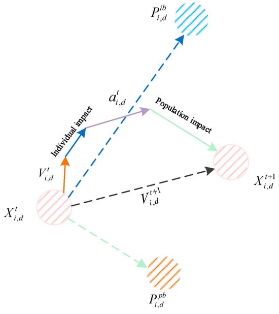
Figure 2.
Improved particle-updating scheme of the IIPSOA-GSA.
- (2)
- Adaptive parameter strategy
The realization of the global optimal solution in relation to the IIPSOA-GSA greatly depends on the parameters related to the inertia weight and setting of learning constants. An equilibrium between global exploration and local exploitation could be achieved by setting an appropriate inertia weight value for the particle. Given this, a dynamic inertia weight is proposed to balance the exploration and exploitation in the algorithm, as shown in (73).
where , , and denote the current function value, the average function value, and the minimum function value. and denote the minimum and maximum values of the inertia weight. It can be observed in (73) that if the fitness function value falls below the average value, it will exhibit better global exploration capability. Conversely, if the fitness function value surpasses the average value, it would demonstrate better local exploitation capability.
The learning constants represent individual knowledge guidance and collective knowledge guidance, meaning a particle can learn from its neighborhood and the best particle in the population. Therefore, an adaptive learning constant strategy was designed to simultaneously enhance global exploration and local exploitation capability, as shown in (74). Considering that learning factors are related to exploration and local exploitation capability at the same time, in the early global exploration phase, would be reduced with iteration, which could weaken the global exploration capability of the population. And, in the exploitation phase, would be increased with iteration, which could improve the local exploitation capability of the population.
6.3. Steps of the Algorithm
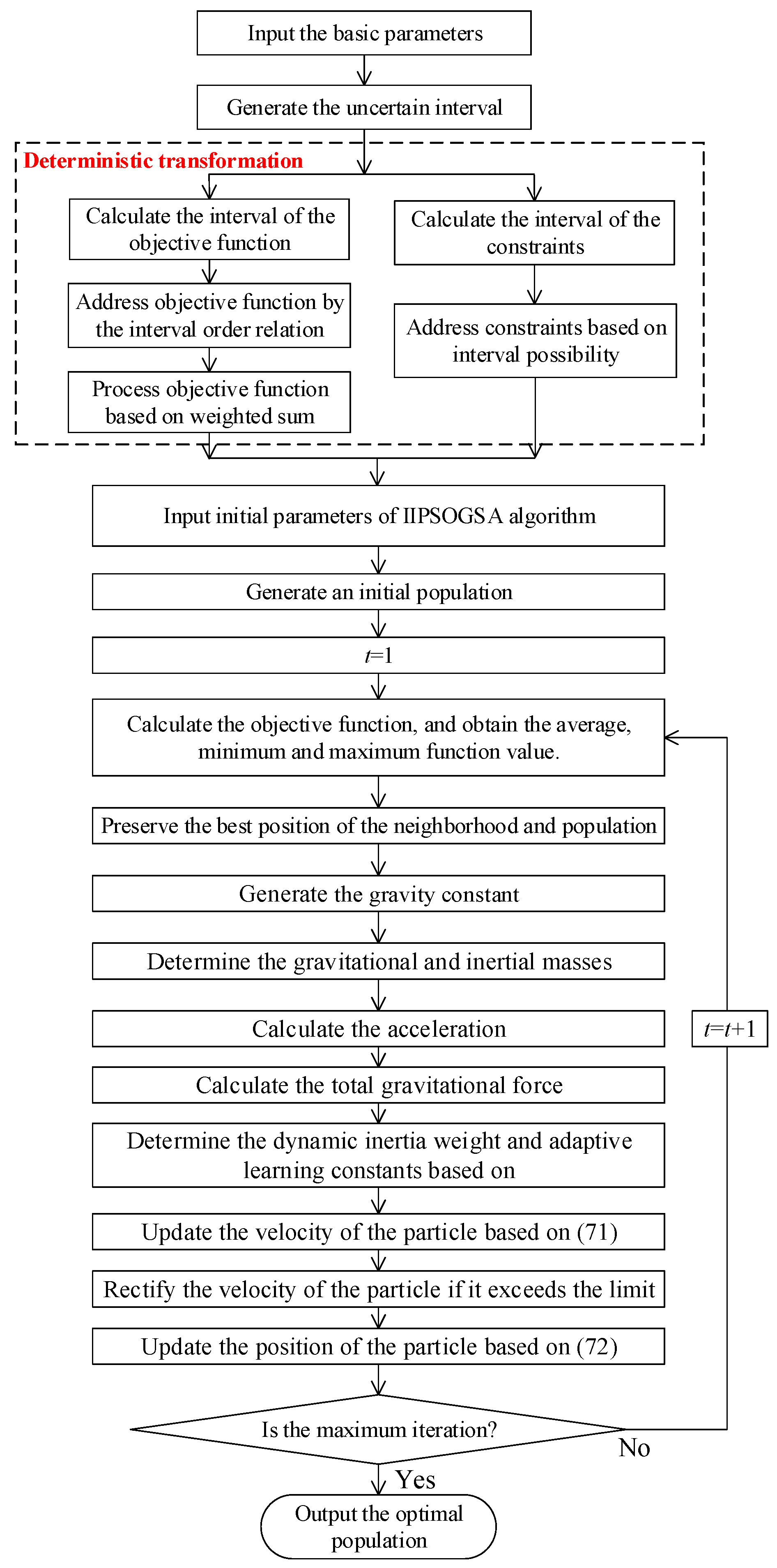
The procedure followed by the proposed IIPSOA-GSA to determine the location and capacity of RESs, the renovation of distribution lines, the site and size of DCs, and the optimal operating strategy is illustrated in Figure 3. The detailed steps of the algorithm are described as follows:

Figure 3.
Flowchart of solution procedures.
Step 1: Input the basic parameters of DCs, RES, and the DN.
Step 2: Generate the uncertain interval concerning the uncertain variables based on the interval-forecasting technique.
Step 3: Implement the deterministic transformation on the IO-based collaborative planning and transform the IOP into a deterministic problem.
Step 4: Input the IIPSOA-GSA related parameters, such as the maximum number of iterations T and the population size N.
Step 5: Generate an initial population corresponding to the RES, DN, and DC investment solutions randomly, i.e., regarding the position and velocity of particles.
Step 6: Set t = 1.
Step 7: Calculate the objective function of the individual, and obtain the average function value, the minimum function value, and the maximum function value.
Step 8: Preserve the best position of the neighborhood particle and the population.
Step 9: Generate the gravity constant based on (62), the gravitational and inertial masses based on (68)–(70), the acceleration based on (65), and the total gravitational force based on (64).
Step 10: Calculate the dynamic inertia weight (73) and adaptive learning constants based on (74).
Step 11: Update the velocity of the particle based on (71).
Step 12: Rectify the particle’s velocity if it exceeds the limit.
Step 13: Update the particle’s position based on (72).
Step 14: If the maximal number of iterations is reached, output the optimal solution. Otherwise, revert to step 2.
7. Case Study
7.1. Test System and Parameters
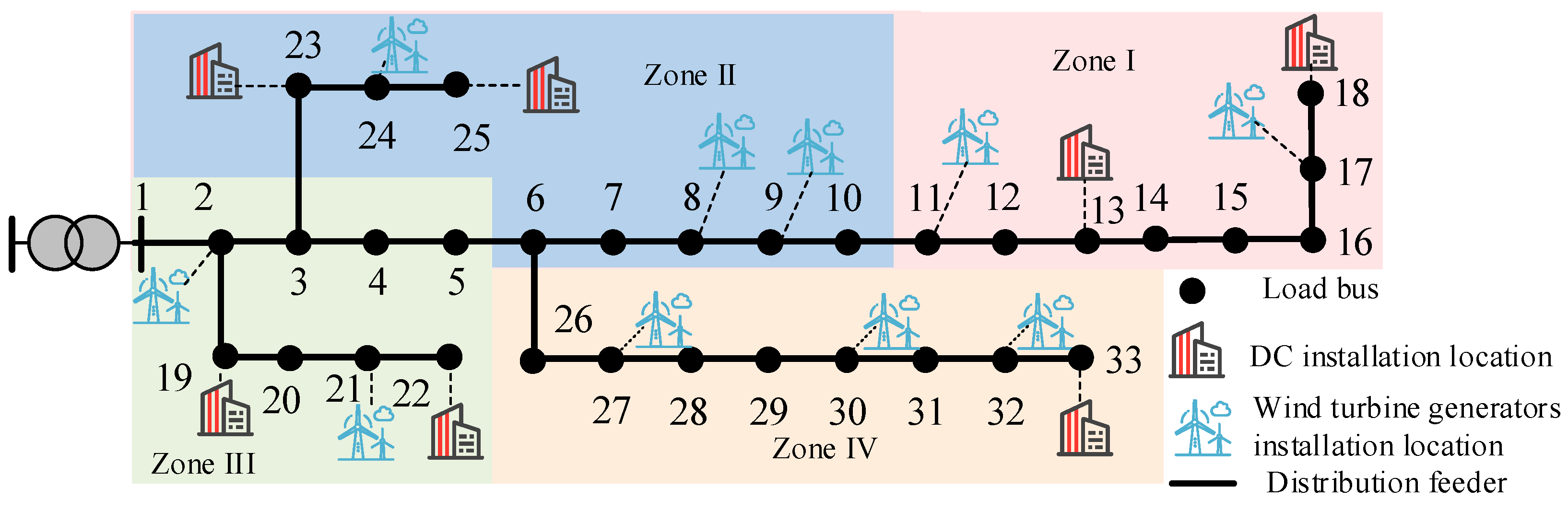
To validate the applicability of the presented planning framework, a case simulation was performed utilizing the improved IEEE-33 bus DN. It is segmented into four zones, where each zone intends to host a DC to meet its workload, with the assumed installation locations being {13,18}, {19,22}, {23,25}, and {26,33} (Figure 4).
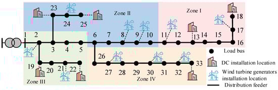
Figure 4.
Modified IEEE 33-bus distribution network.
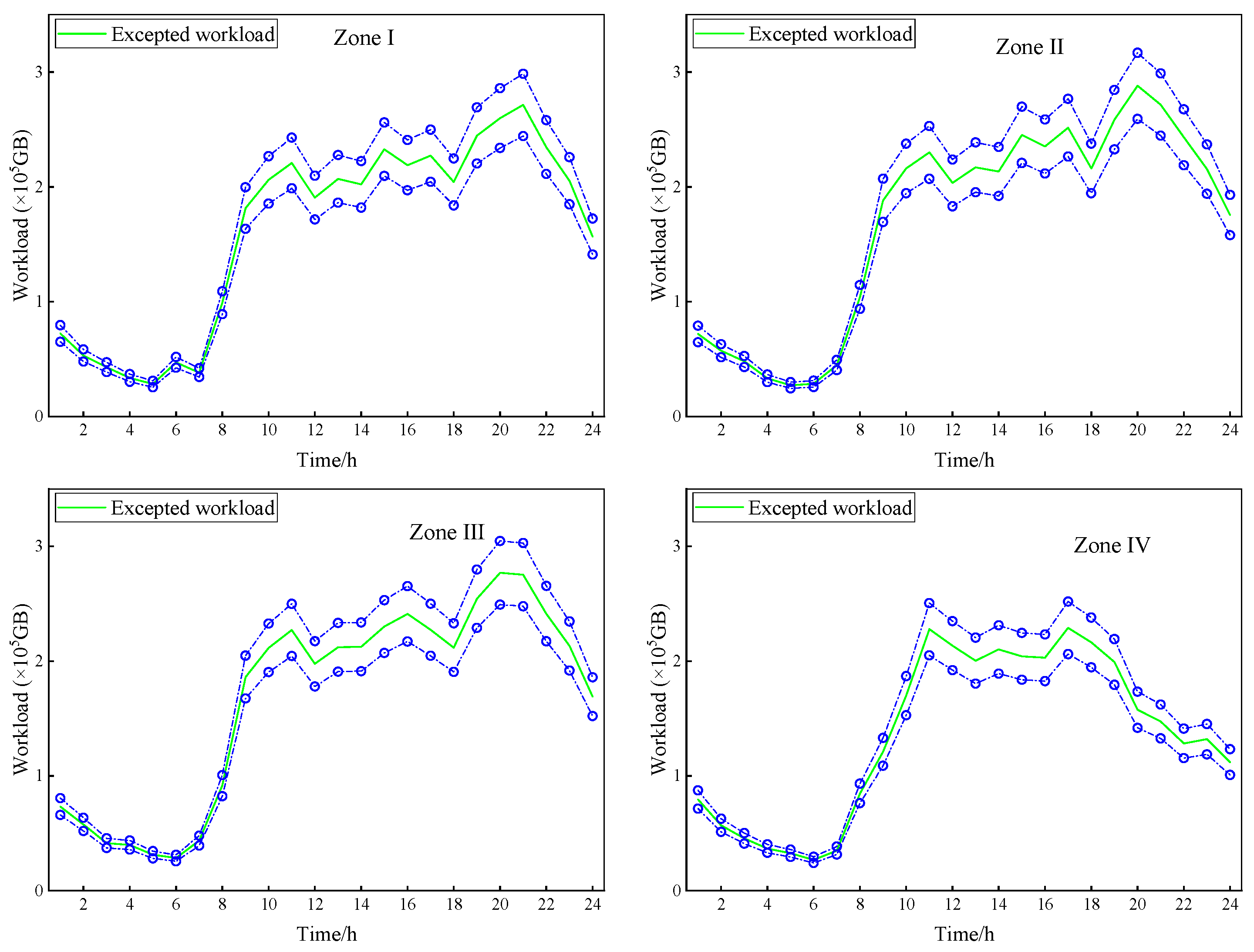
In the DC simulation, the indoor temperature is set to a range of 5–25 °C. A maximum delay of 500 ms is assigned to workloads [38], and the ratio of DW to RW is set at 4:1. The workloads are ascertained with a ±10% uncertainty interval [5], as depicted in Figure 5.
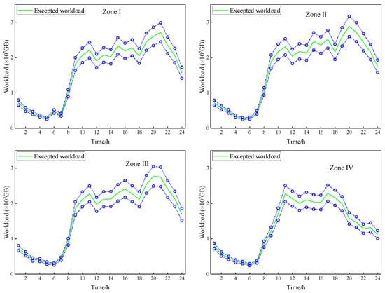
Figure 5.
Uncertain parameter interval predictions of workloads, where the bule lines are the upper and lower bounds of workloads.
The corresponding parameters of different components are presented in Table 2. The expansion expense of the distribution transformer was set to RMB/MVA 2M (RMB/MVA represents million Chinese Renminbi (RMB) per megavolt-ampere (MVA)). DC and distribution line parameters are presented in Table 3 and Table 4.
Table 2.
Basic parameters of components related to planning.
Table 3.
Settings of DC parameters.
Table 4.
Parameters of feeders.
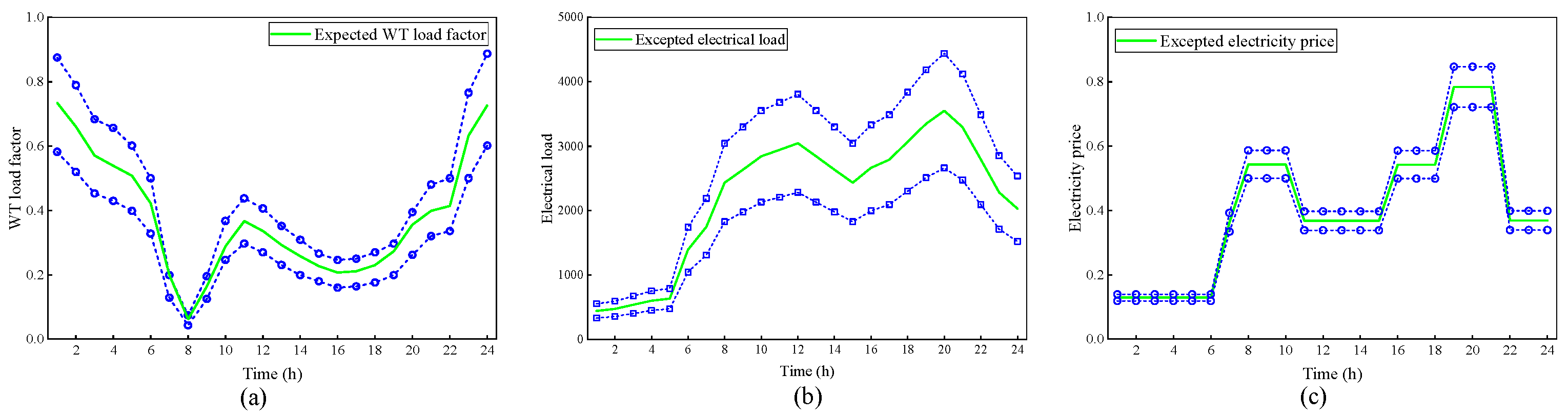
Utilizing recorded actual wind speed data, the expected load factor is ascertained, considering an interval range of ±20%, which is depicted in Figure 6a. We determine the electrical load with ±20% uncertain boundaries, as shown in Figure 6b. The electricity price is also presented in Figure 6c, and the predicted emissions coefficient is 0.899, with a ±10% uncertainty limit [34,39].
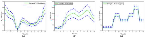
Figure 6.
Intervals of uncertainty variable, where the bule lines are the upper and lower bounds of uncertainties: (a) RES load factor; (b) power load; and (c) electricity price.
Based on the previous test, the relevant parameters of the algorithm were set as follows: = 0.4, = 0.9, = = 2.5, = = 0.5, G0 = 100, and = 0.2.
7.2. Results of the Experiments
To expound on the advantages of collaborative planning between DCs and DNs, a comparison is presented examining three distinct cases.
Case I: Independent planning for the DCs, RES, and DN. In this scenario, it is presumed that the locations of DCs remain stationary, and there is no interaction between DCs and the DN.
Case II: Collaborative planning for the DCs, RES, and DN, in which the DCs do not provide flexibility.
Case III: The proposed planning model.
Utilizing the suggested methodology, the planning performance and solutions in different cases were shown in Table 5 and Table 6.
Table 5.
Planning performance in different cases.
Table 6.
Optimal planning solutions in different cases.
The comparison between Cases I and II affirms the validity of the collaborative planning. Case I, with a higher RES capacity, exhibits elevated costs and emissions compared to Case II corroborating our prediction of suboptimal DC station positioning. Conversely, Case II’s integrated planning fosters synergistic RES and DC planning by assessing their collective impact on DN operations.
Furthermore, the analysis of Cases II and III underscores the significant impact of harnessing the demand response of DCs. As evidenced by Table 5, Case III exhibits notably superior system benefit compared to Case II. And, the diminished RES capacity in Case III, relative to Case II, indicates the investment reduction could be achieved through optimizing workload distribution, minimizing DC power consumption, and enhancing load curves. These measures collectively result in a reduction in the investment of servers, ACE. By fully leveraging DC operating flexibility, the operator can enhance RES utilization and decrease reliance on high-carbon external market electricity. Conversely, in Case II, the infeasible rescheduling of DCs workload demand leads to elevated consumption, particularly during peak demand and low RES generation, necessitating additional RES capacity allocation and external grid electricity procurement.
7.3. Discussion
7.3.1. Performance of DC Demand Response
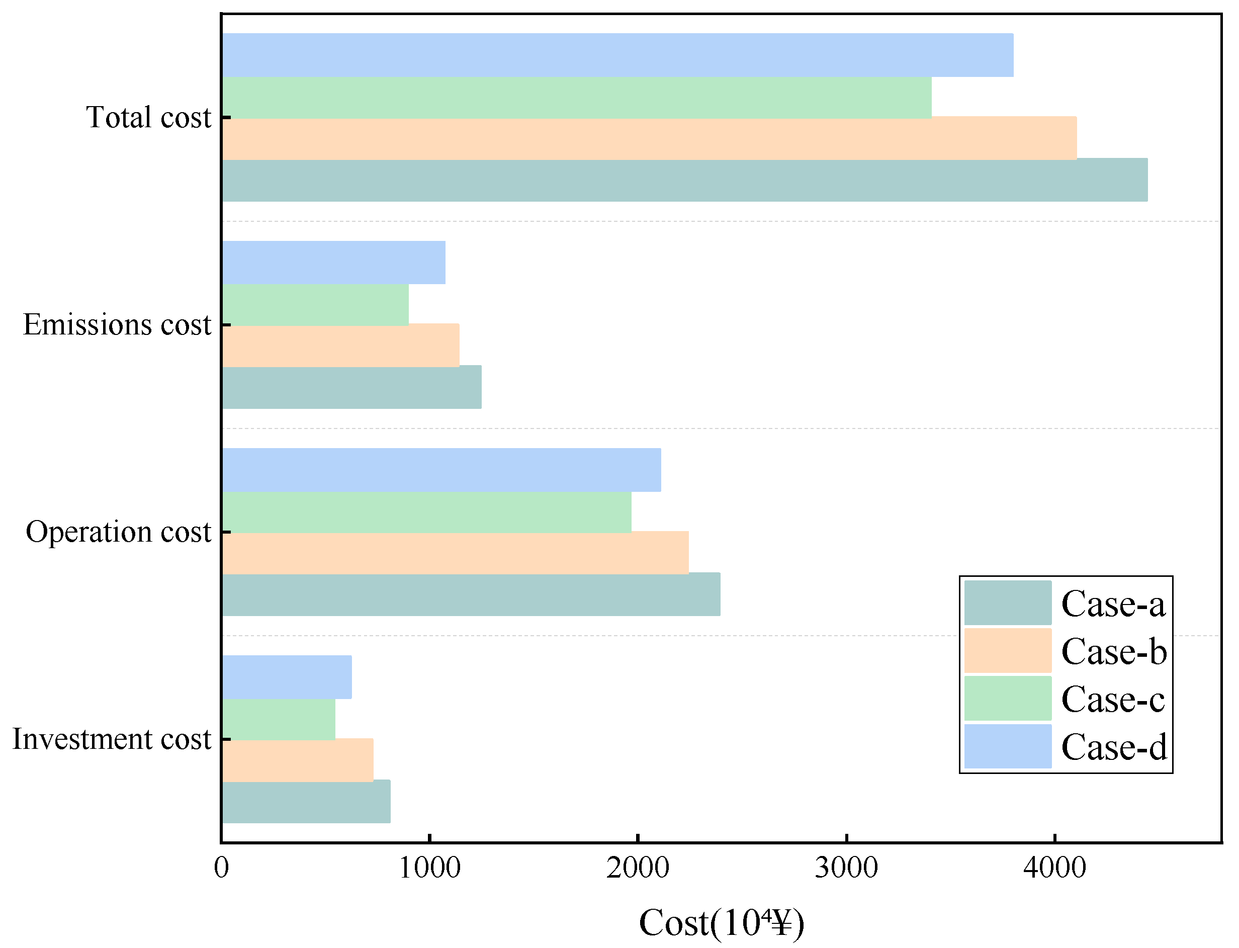
In that research, the operational flexibility of DCs was considered. To demonstrate the influence of flexibility, four cases were defined to facilitate an assessment.
Case a: Ignore the DW and RW in the DC modeling.
Case b: Only DW is taken into account.
Case c: DW and RW are considered at the same time. It is noteworthy that Cases aߝc all consider the thermal inertia in DC building.
Case d: Both DW and RW are taken into account. But thermal inertia is exclusive with the indoor temperature is fixed at 20 °C.
The results of the above four cases are shown in Figure 7. As can be seen, the most favorable outcomes, characterized by the minimal economic cost, are observed in Case c. Subsequently, Case d and Case b perform relatively better, albeit not as optimal as Case c. On the other hand, Case a is associated with the least-desirable results. These findings underscore the significant potential of leveraging DC flexibility to enhance the system benefits.
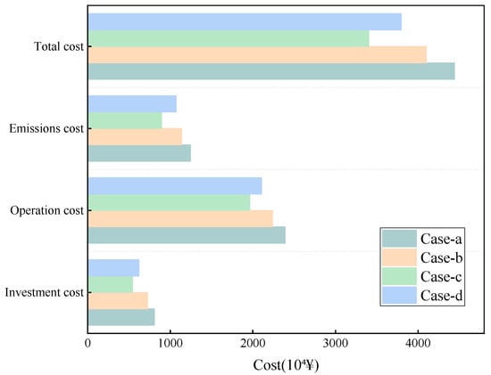
Figure 7.
Comparison of performance in the four cases.
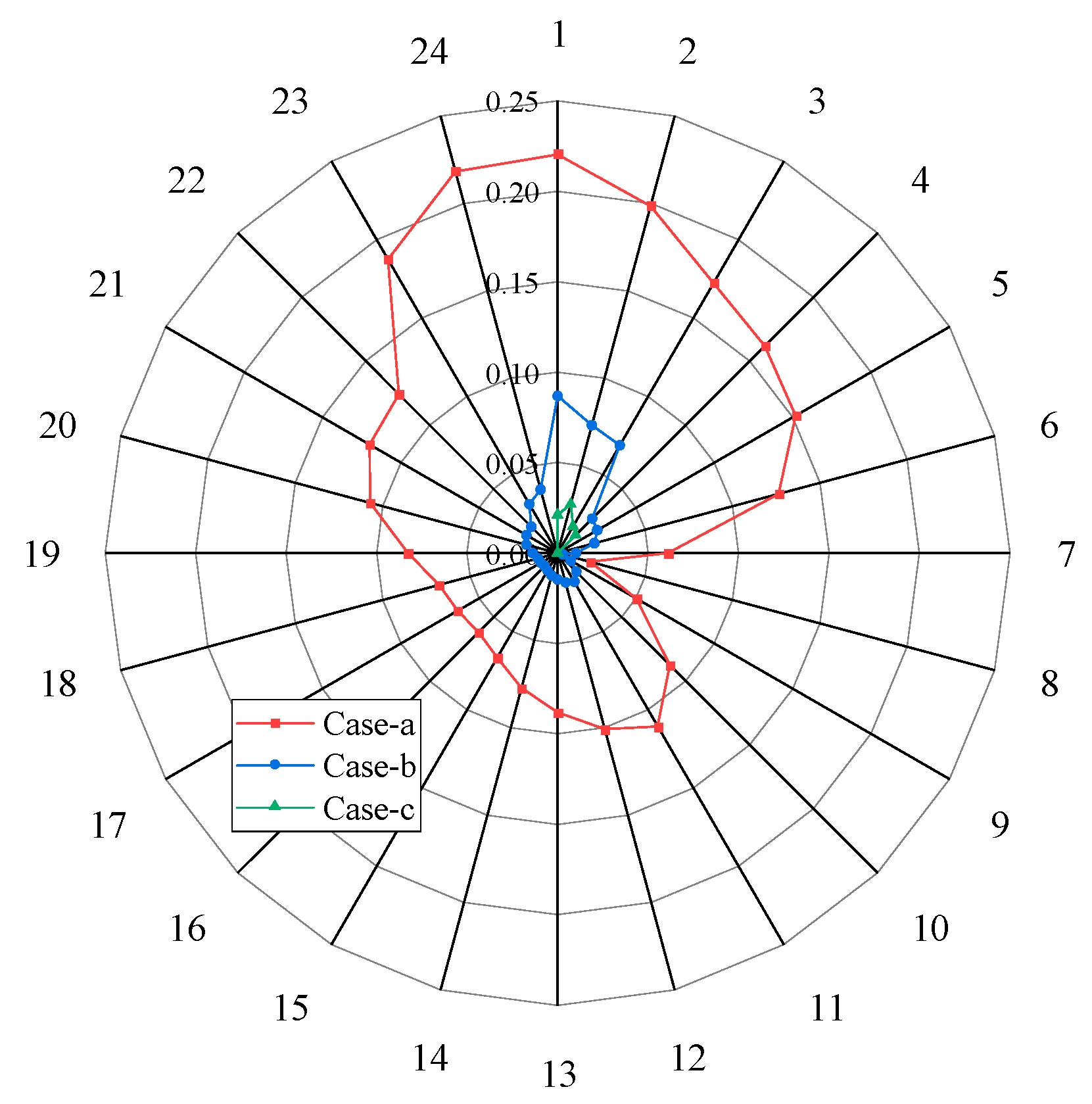
To further elucidate the practical effect of the temporal and spatial distribution of DC workloads on the enhancement of DN benefits, the dispatching results of the RES curtailment and active servers under Cases a-c are illustrated in Figure 8 and Figure 9, respectively. As shown in Figure 8, when the DC does not participate in scheduling workloads (Case a), a notable mismatch exists between RES and DC power consumption, which results in significant curtailment. In particular, considering the temporal and spatial distribution of DC workloads simultaneously, the utilization rate of RESs further increases compared to Cases b and c.
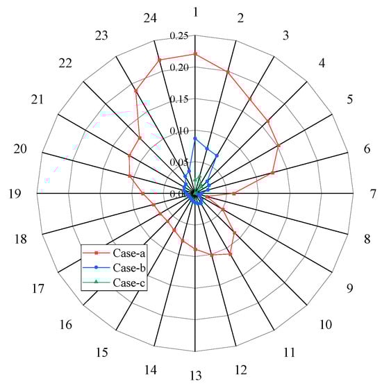
Figure 8.
Wind power curtailment in cases a–c.
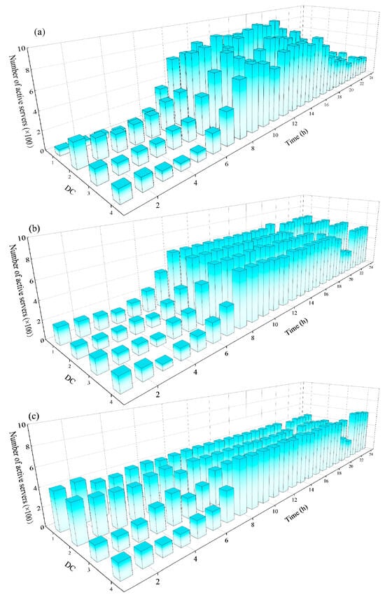
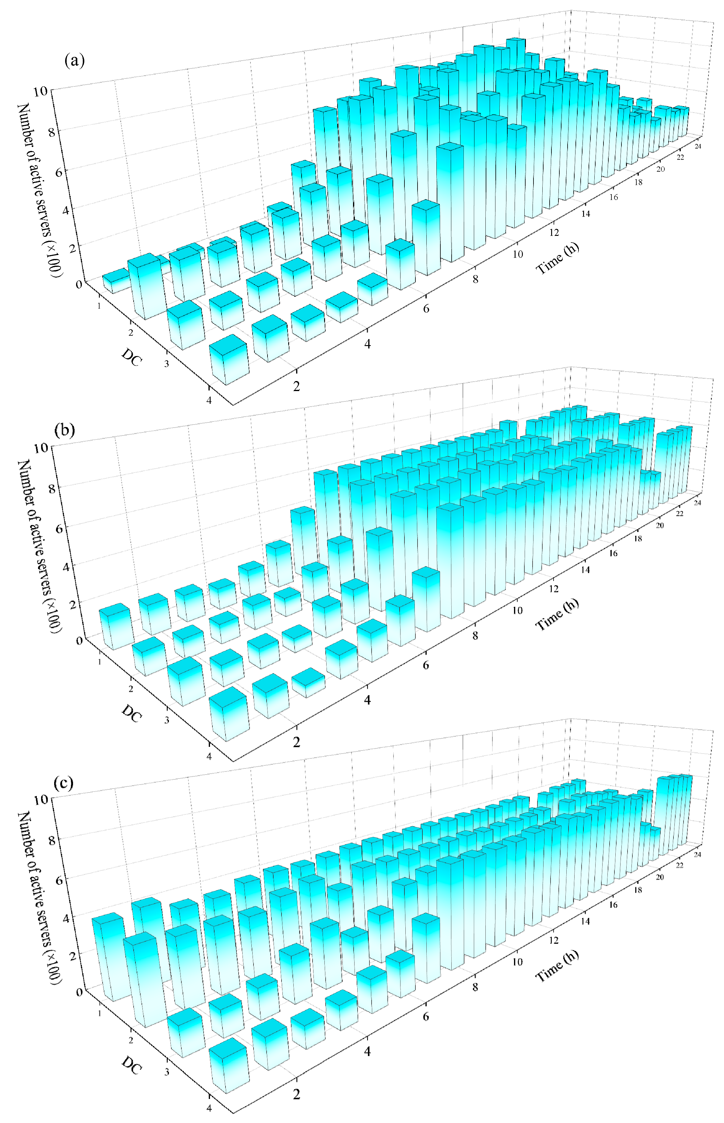
Figure 9.
Number of active servers: (a) Case a; (b) Case b; (c) Case c.
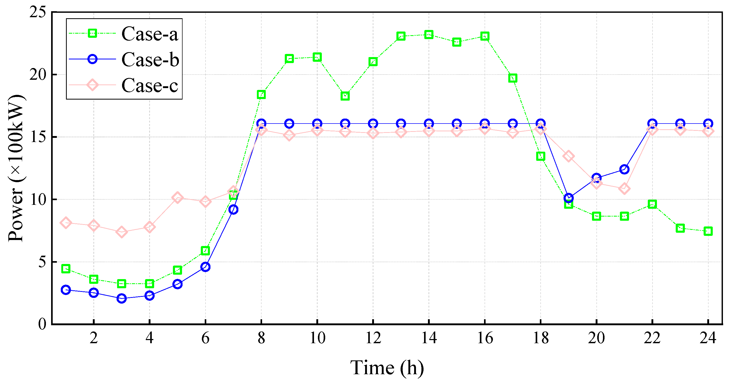
The dispatching results of the active servers in Figure 9 further confirm the point made above: in Case b, the workload originally scheduled from 08:00 to 17:00 is deferred to the period from 18:00 to 24:00, aligning with high wind power generation intervals. This adjustment leads to a reduction in the RES curtailment rate, decreasing from 11.66% to 9.1%. But, since DW solely modifies the power consumption on time, wind curtailment persists during the hours of 01:00 to 05:00. Conversely, Case c, which considers both DW and RW simultaneously, increases the number of operating servers in DC1 and DC2, thereby further enhancing the consumption efficiency of renewable energy so as to transfer more workloads to zone 1 and 2, improving both economic and environmental benefits. In addition, the total DC power consumption in Cases a–c is shown in Figure 10. As can be seen, the total DC power consumption in Case c matches the RES output to a greater extent, and the difference between peak and valley in each period is smaller. On the contrary, the difference between the peak and valley in each period with respect to the power consumption in Case c is significantly large. The above analysis demonstrates that if a DC fully uses the temporal and spatial flexibility of its workloads, greater efficiency can be obtained.
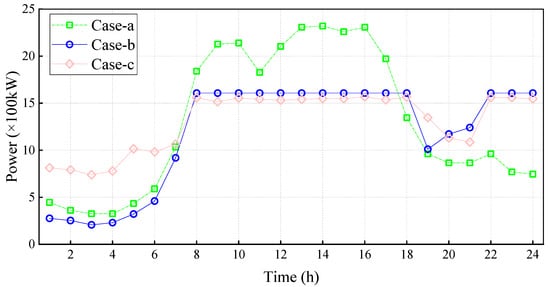
Figure 10.
Toal DC power consumption: Case a; Case b; Case c.
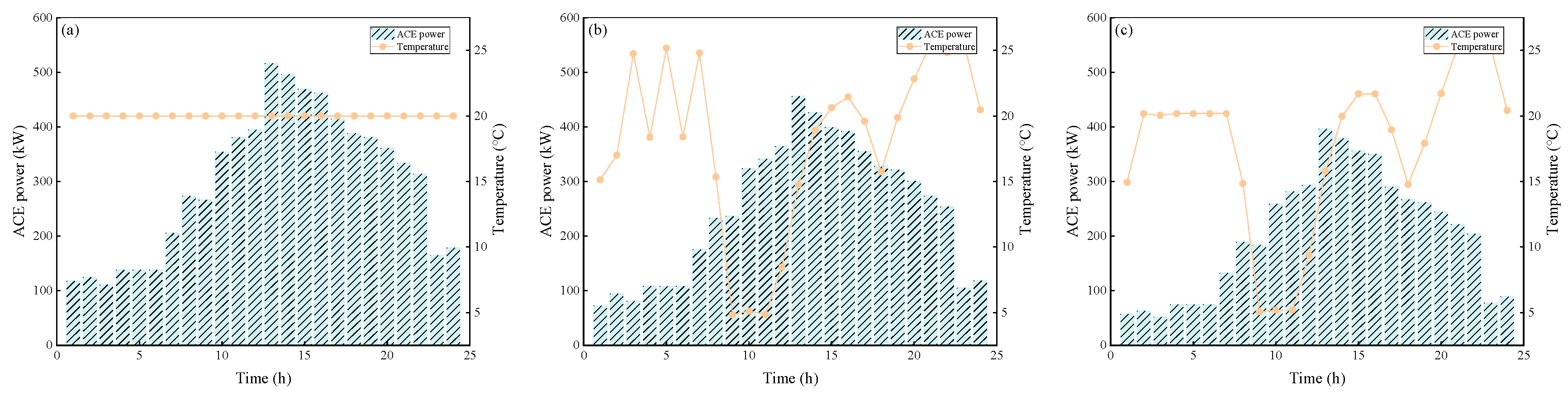
To investigate the impact of the thermal inertia in DC building, we determined the impact of the thermodynamic process on indoor temperature variations, as Figure 11 illustrates. Once thermal inertia is disregarded, the ambient temperature remains stable at 20 °C without any fluctuations, which could lead to high cooling power consumption. However, with thermal inertia considered, the temperature in Case d exhibits fluctuations in a tolerable limit. This characteristic potentially enables the deployment of an ACE to reduce cooling consumption. Therefore, leveraging the thermal inertia allows for the relaxation of constraints on indoor temperature, which could allow the dispatch of a cooling system that is as flexible as possible to provide support for the DN.
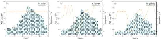
Figure 11.
DC temperature and ACE power: (a) Case d; (b) Case a; (c) Case c.
7.3.2. Performance of the Proposed Algorithm
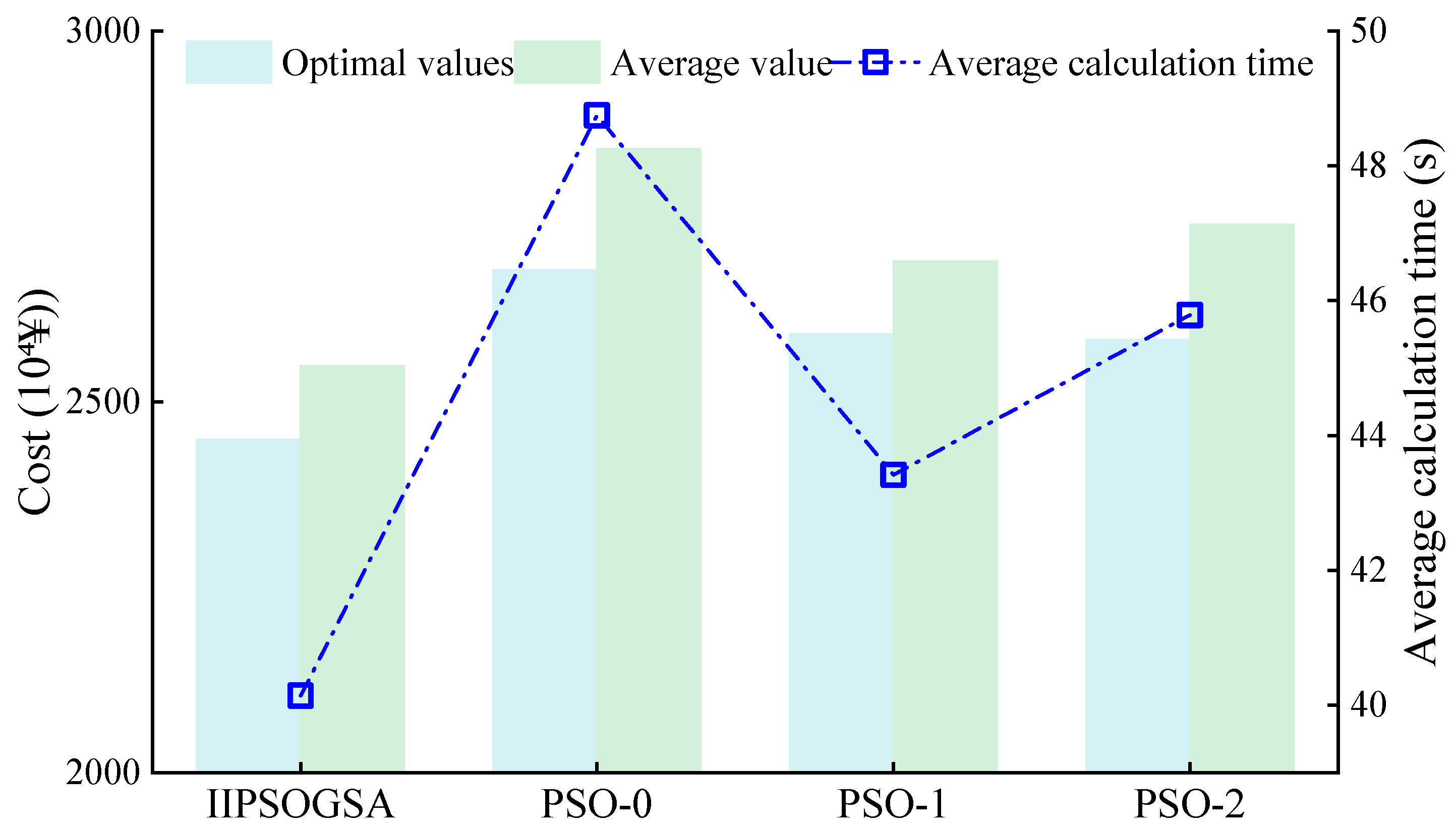
To illustrate the advantage of the proposed IIPSOA-GSA, in this section, this algorithm is compared with the traditional PSO (PSO-0), modified PSO-1 [40], and modified PSO-2 [41]. For the PSO-0, was set to 1, and h1 and h2 were both set to 2. The corresponding parameters of PSO-1 and PSO-2 were derived from the literature. The above four algorithms were utilized to solve the collaborative planning model over 100 runs. The results concerning the average calculation time and the optimal and average values are presented in Figure 12.
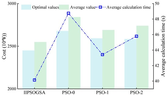
Figure 12.
Comparison of algorithm performance.
As observed, the optimal values for the IIPSOA-GSA are 9.32%, 5.76%, and 5.47% lower than those of PSO-0, PSO-1, and PSO-2, respectively. The average objective function values are 11.5%, 5.53%, and 7.50% lower than those of PSO-0, PSO-1, and PSO-2, respectively. At the same time, compared to PSO-0, PSO-1, and PSO-2, the IIPSOA-GSA demonstrates a shorter average computation time, which shows that the IIPSOA-GSA algorithm has stronger search ability and can provide better choices for system operators when planning.
8. Imitations of the Proposed Framework
This research endeavor possesses certain limitations that we intend to address in subsequent studies. First, the proposed planning model is assumed to be implemented under a centralized setting, wherein the planning and operation of all the system components (including data centers, the distribution network, and the RES) are performed by a single entity. However, in real-world situations, this assumption may not be tenable as system planning and operation may involve different market players. In this case, it is meaningful to establish a decentralized optimization framework to ensure the profitability of different stakeholders while respecting the system’s constraints. Furthermore, for the sake of practicability, the impacts of information networks should also be considered in DC modeling.
9. Conclusions and Future Work
This paper presents an IO-based framework for the coordinated planning of data centers, RESs, and DNs within the context of low-carbon development. The presented model considers the flexibility characteristics of DCs, thereby harnessing their latent flexibility. Through the utilization of an interval optimization method, it explicitly integrates the influence of uncertainties. A deterministic transformation approach and an IIPSOA-GSA were developed to solve the proposed model effectively. A case study on the modified IEEE 33-bus system was conducted, leading to the following conclusions.
(a): The proposed collaborative planning framework can reduce the total annualized cost by 35.29%. Additionally, the operational flexibility of DCs in the proposed planning model greatly impacts the planning results. For instance, relative to the model that does not consider flexibility, there were 46.2% and 40% drops in the capacities of servers and ACE, respectively, in the proposed planning model.
(b): The coordinated energy management of DCs and the corresponding DN can significantly promote RES utilization via the flexible utilization of the spatiotemporal characteristics of workloads. Considering the spatio-temporal scheduling of workloads, the RES curtailment rate can be reduced by 91.2%. Furthermore, integrating thermal inertia into DC management facilitates more adaptable cooling strategies, resulting in cost savings and carbon emission reductions of 11.5% and 19.8%, respectively.
(c): After comparing the different algorithms, the optimal values attained by the proposed IIPSOA-GSA exhibited reductions of 9.32%, 5.76%, and 5.47% compared to those of PSO-0, PSO-1, and PSO-2, respectively. Additionally, the average objective function value for IIPSOA-GSA was 11.5%, 5.53%, and 7.50% lower than that for PSO-0, PSO-1, and PSO-2, respectively. These findings indicate that the proposed IIPSOA-GSA possesses superior search capabilities, furnishing system operators with more optimal planning alternatives.
This research focused on the collaborative planning of DCs, RESs and DNs from a single power system setting. In the real world, the data center is an emerging power consumption subject that integrates the use and transformation of various energy sources, e.g., electricity, cooling, and heating. In the future, the collaborative planning of data centers, renewable energy resources, and energy networks will be exploited from a holistic multi-energy system viewpoint.
Author Contributions
Conceptualization, L.S. and W.W.; methodology, W.F.; software L.S.; validation, J.Q., Y.A. and L.S.; formal analysis, L.S.; investigation, W.W.; resources, W.F.; data curation, W.F.; writing—original draft preparation, L.S., W.W., W.F., J.Q.; writing—review and editing, J.Q.; visualization, Y.A.; supervision, Y.A.; project administration, L.S.; funding acquisition, L.S. All authors have read and agreed to the published version of the manuscript.
Funding
This work was funded by the Science and Technology Project of State Grid Hubei Electric Power Co., Ltd. (Grant number: B31532236158).
Data Availability Statement
The data presented in this study are available on request from the corresponding author. The data are not publicly available due to confidentiality.
Conflicts of Interest
Authors Lei Su, Wanli Feng and Yuqi Ao were employed by the State Grid Hubei Electric Power Research Institute. Authors Wenxiang Wu and Junda Qin were employed by the company State Key Laboratory of Advanced Power Transmission Technology, State Grid Smart Grid Research Institute Co., Ltd. The authors declare that the research was conducted in the absence of any commercial or financial relationships that could be construed as a potential conflict of interest.
Nomenclature
| Indicates (Sets) | |
| i | Load node |
| d | DC node |
| t | Time periods |
| j | RES node |
| Variables | |
| Data workload capacity transferred from time t to time t’ | |
| Number of data transferred between the two DCs | |
| Quantity of DW/RW data at the end of scheduling | |
| Waiting time for data workloads in the queue | |
| Data-processing time | |
| Indoor/outdoor temperature of the DC | |
| Upper and lower bounds of the indoor temperature of the DC | |
| Indoor-temperature variation rates of the data center | |
| Total active power consumption of the DC at time t for node d | |
| Active power of servers / ACE | |
| Number of servers in the powered-on state at time t | |
| Number of installed servers | |
| Maximum CPU utilization | |
| Cooling power of the DC | |
| ACE installation capacity | |
| Capacity expansion of the distribution transformer | |
| Investment cost for equipment X | |
| Investment cost for the distribution line | |
| Binary variable representing the linear selection | |
| Length of the line | |
| Purchased power from the main grid | |
| Purchase price of electricity | |
| Cost coefficient for DW participating in demand response | |
| Intensity of carbon emissions for electricity production on the grid side | |
| Maximum expansion capacity of the substation | |
| Maximum installation number of equipment X | |
| / | Active/reactive power flowing through line ij at time t |
| Active/reactive power of the load at time t | |
| Reactive power of RES/DC at time t | |
| Maximum/minimum allowable voltage values at node i | |
| / | Resistance/reactance of line ij |
| Capacities of line ij before and after the transformation | |
| Uncertain variables | |
| Interval of RES load factor | |
| Interval of electricity price | |
| Interval of carbon emission coefficient | |
| Interval of electric load demand | |
| Interval of workloads | |
| Parameters | |
| Ratio of DW/RW in the total data workloads | |
| Initial amount of DW/RW | |
| The maximum allowable delay time for users | |
| Air density | |
| Specific heat capacity of air | |
| Wall area of the DC room | |
| The unit wall heat exchange coefficient | |
| Operating heat dissipation coefficient of the equipment | |
| Energy efficiency coefficient of the DC/ACE | |
| Average utilization of the server | |
| Server processing rate | |
| Server spare coefficient | |
| Standby/peak power consumption of a single server |
References
- Koot, M.; Wijnhoven, F. Usage impact on data center electricity needs: A system dynamic forecasting model. Appl. Energy 2021, 291, 116798. [Google Scholar] [CrossRef]
- Ting, Y.; Han, J.; Yucheng, H. Study on carbon neutrality regulation method of interconnected multi-datacenter based on spatio-temporal dual-dimensional computing load migration. Proc. CSEE 2022, 42, 164–177. [Google Scholar]
- Li, C.; Yan, Z.; Yao, Y.; Deng, Y.; Shao, C.; Zhang, Q. Coordinated low-carbon dispatching on source-demand side for integrated electricity-gas system based on integrated demand response exchange. IEEE Trans. Power Syst. 2024, 39, 1287–1303. [Google Scholar] [CrossRef]
- Zhu, X.; Zhan, X.; Sun, Y.; Zhang, Y. Cloud-edge collaborative distributed optimal dispatching strategy for an electric-gas integrated energy system considering carbon emission reductions. Int. J. Electr. Power Energy Syst. 2022, 143, 108458. [Google Scholar] [CrossRef]
- Chen, M.; Gao, C.; Shahidehpour, M.; Li, Z.; Chen, S.; Li, D. Internet data center load modeling for demand response considering the coupling of multiple regulation methods. IEEE Trans. Smart Grid 2021, 12, 2060–2076. [Google Scholar] [CrossRef]
- Sakanova, A.; Alimohammadi, S.; McEvoy, J.; Battaglioli, S.; Persoons, T. Multi-objective layout optimization of a generic hybrid-cooled data centre blade server. Appl. Therm. Eng. 2019, 156, 514–523. [Google Scholar] [CrossRef]
- Ajmal, M.S.; Iqbal, Z.; Khan, F.Z.; Bilal, M.; Mehmood, R.M. Cost-based energy efficient scheduling technique for dynamic voltage and frequency scaling system in cloud computing. Sustain. Energy. Technol. 2021, 45, 101210. [Google Scholar]
- Arshad, U.; Aleem, M.; Srivastava, G.; Lin, J. Utilizing power consumption and SLA violations using dynamic VM consolidation in cloud data centers. Renew. Sustain. Energy Rev. 2022, 167, 112782. [Google Scholar] [CrossRef]
- Qu, S.; Duan, K.; Guo, Y.; Feng, Y.; Wang, C.; Xing, Z. Real-time optimization of the liquid-cooled data center based on cold plates under different ambient temperatures and thermal loads. Appl. Energy 2024, 363, 123101. [Google Scholar] [CrossRef]
- Zou, Z.; Yang, C.; Hu, L.; Zhang, Q. A novel data center free radiating system driven by waste heat and wind energy system (DCFRWWs) and its operation performance analysis. Energy Build. 2024, 310, 114061. [Google Scholar]
- Chen, T.; Wang, X.; Giannakis, G.B. Cooling-aware energy and workload management in data centers via stochastic optimization. IEEE J. Sel. Top. Signal Process 2015, 10, 402–415. [Google Scholar] [CrossRef]
- Chen, S.; Li, P.; Ji, H.; Hao, Y.; Ji, H.; Wu, J.; Wang, C. Operational flexibility of active distribution networks with the potential from data centers. Appl. Energy 2021, 293, 116935. [Google Scholar] [CrossRef]
- Liu, X. Research on collaborative scheduling of internet data center and regional integrated energy system based on electricity-heat-water coupling. Energy 2024, 292, 130462. [Google Scholar] [CrossRef]
- Han, O.; Ding, T.; Mu, C.; Jia, W.; Ma, Z. Coordinative optimization between multiple data center operators and a system operator based on two-level distributed scheduling algorithm. IEEE Internet Things J 2023, 10, 7517–7527. [Google Scholar] [CrossRef]
- Lian, T.; Li, Y.; Zhao, Y.; Yu, C.; Zhao, T.; Wu, L. Robust multi-objective optimization for islanded data center microgrid operations. Appl. Energy 2023, 330, 120344. [Google Scholar] [CrossRef]
- Huang, S.; Yan, D.; Chen, Y. An online algorithm for combined computing workload and energy coordination within a regional data center cluster. Int. J. Electr. Power Energy Syst. 2024, 158, 109971. [Google Scholar] [CrossRef]
- Xiao, J.; Yang, Y.; Cui, S.; Wang, Y. Cooperative online schedule of interconnected data center microgrids with shared energy storage. Energy 2023, 285, 129522. [Google Scholar] [CrossRef]
- Liu, W.; Yan, Y.; Sun, Y.; Mao, H.; Cheng, M.; Wang, P.; Ding, Z. Online job scheduling scheme for low-carbon data center operation, An information and energy nexus perspective. Appl. Energy 2023, 338, 120918. [Google Scholar] [CrossRef]
- Wu, Z.; Lin, C.; Wang, J.; Zhou, M.; Li, G.; Xia, Q. Incentivizing the spatiotemporal flexibility of data centers toward power system coordination. IEEE Trans. Netw. Sci. Eng. 2023, 10, 1766–1778. [Google Scholar] [CrossRef]
- Wang, J.; Deng, H.; Liu, Y.; Guo, Z.; Wang, Y. Coordinated optimal scheduling of integrated energy system for data center based on computing load shifting. Energy 2023, 267, 126585. [Google Scholar] [CrossRef]
- Wan, T.; Tao, Y.; Qiu, J.; Lai, S. Internet data centers participating in electricity network transition considering carbon-oriented demand response. Appl. Energy 2023, 329, 120305. [Google Scholar] [CrossRef]
- Qi, W.; Li, J.; Liu, Y.; Liu, C. Planning of distributed internet data center microgrids. IEEE Trans. Smart Grid 2017, 10, 762–771. [Google Scholar] [CrossRef]
- Liu, J.; Xu, Z.; Wu, J.; Liu, K.; Sun, X.; Guan, X. Optimal planning of internet data centers decarbonized by hydrogen-water-based energy systems. IEEE Trans. Autom. Sci. Eng. 2022, 20, 1577–1590. [Google Scholar] [CrossRef]
- Li, W.; Qian, T.; Zhang, Y.; Shen, Y.; Wu, C.; Tang, W. Distributionally robust chance-constrained planning for regional integrated electricity–heat systems with data centers considering wind power uncertainty. Appl. Energy 2023, 336, 120787. [Google Scholar] [CrossRef]
- Vafamehr, A.; Khodayar, M.E.; Manshadi, S.D.; Ahmad, I.; Lin, J. A framework for expansion planning of data centers in electricity and data networks under uncertainty. IEEE Trans. Smart Grid 2017, 10, 305–316. [Google Scholar] [CrossRef]
- Zeng, B.; Xu, F.; Liu, Y.; Gong, D.; Zhu, X. Multi-objective interval optimization approach for energy hub planning with consideration of renewable energy and demand response synergies. Proc. CSEE 2021, 41, 7212–7224. [Google Scholar]
- Li, Y.; Wang, P.; Gooi, H.; Ye, J.; Wu, L. Multi-objective optimal dispatch of microgrid under uncertainties via interval optimization. IEEE Trans. Smart Grid 2019, 10, 2046–2058. [Google Scholar] [CrossRef]
- Jiang, T.; Li, X.; Kou, X.; Zhang, R.; Tian, G.; Li, F. Available transfer capability evaluation in electricity-dominated integrated hybrid energy systems with uncertain wind power: An interval optimization solution. Appl. Energy 2022, 314, 119001. [Google Scholar] [CrossRef]
- Su, Y.; Zhou, Y.; Tan, M. An interval optimization strategy of household multi-energy system considering tolerance degree and integrated demand response. Appl. Energy 2020, 260, 114144. [Google Scholar] [CrossRef]
- Wang, W.; Dong, H.; Luo, Y.; Zhang, C.; Zeng, B.; Xu, F.; Zeng, M. An Interval Optimization-Based Approach for Electric–Heat–Gas Coupled Energy System Planning Considering the Correlation between Uncertainties. Energies 2021, 14, 2457. [Google Scholar] [CrossRef]
- Song, J.; Zhang, Z.; Mu, Y.; Wang, X.; Chen, H.; Pan, Q.; Li, Y. Enhancing environmental sustainability via interval optimization for low-carbon economic dispatch in renewable energy power systems: Leveraging the flexible cooperation of wind energy and carbon capture power plants. J. Clean. Prod. 2024, 442, 140937. [Google Scholar] [CrossRef]
- Wang, P.; Cao, Y.; Ding, Z.; Tang, H.; Wang, X.; Cheng, M. Stochastic programming for cost optimization in geographically distributed internet data centers. CSEE JPES 2022, 8, 1215–1232. [Google Scholar]
- Chinese Grids’ Transformation to Benefit Digital&Tech Companies Globally. Available online: https://energyiceberg.com (accessed on 13 April 2024).
- Dong, H.; Wang, L.; Zhang, X.; Zeng, M. A two-stage stochastic collaborative planning approach for data centers and distribution network incorporating demand response and multivariate uncertainties. J. Clean. Prod. 2024, 451, 141482. [Google Scholar] [CrossRef]
- Zeng, B.; Wang, W.; Zhang, W.; Wang, Y.; Tang, C.; Wang, J. Optimal configuration planning of vehicle sharing station-based electro-hydrogen micro-energy systems for transportation decarbonization. J. Clean. Prod. 2023, 387, 135906. [Google Scholar] [CrossRef]
- Lei, G.; Xu, C. Optimal intelligent reconfiguration of distribution network in the presence of distributed generation and storage system. Energy Eng. 2024, 119, 2005–2029. [Google Scholar] [CrossRef]
- Rashedi, E.; Nezamabadi-pour, H.; Saryazdi, S. GSA: A Gravitational Search Algorithm. Inf. Sci. 2009, 179, 2232–2248. [Google Scholar] [CrossRef]
- Zhao, Z.; Fan, L.; Han, Z. Optimal data center energy management with hybrid quantum-classical multi-cuts benders’ decomposition method. IEEE Trans. Sustain. Energy 2024, 15, 847–858. [Google Scholar] [CrossRef]
- Zeng, B.; Zhang, W.; Hu, P.; Sun, J.; Gong, D. Synergetic renewable generation allocation and 5G base station placement for decarbonizing development of power distribution system: A multi-objective interval evolutionary optimization approach. Appl. Energy 2023, 351, 121831. [Google Scholar] [CrossRef]
- Lu, X.; Zhou, K.; Yang, S.; Liu, H. Multi-objective optimal load dispatch of micro-grid with stochastic access of electric vehicles. J. Clean. Prod. 2018, 195, 187–199. [Google Scholar] [CrossRef]
- Lu, X.; Zhou, K.; Yang, S. Multi-objective optimal dispatch of micro-grid containing electric vehicles. J. Clean. Prod. 2017, 165, 1572–1581. [Google Scholar] [CrossRef]
Disclaimer/Publisher’s Note: The statements, opinions and data contained in all publications are solely those of the individual author(s) and contributor(s) and not of MDPI and/or the editor(s). MDPI and/or the editor(s) disclaim responsibility for any injury to people or property resulting from any ideas, methods, instructions or products referred to in the content. |
© 2024 by the authors. Licensee MDPI, Basel, Switzerland. This article is an open access article distributed under the terms and conditions of the Creative Commons Attribution (CC BY) license (https://creativecommons.org/licenses/by/4.0/).