Planning a Hybrid Battery Energy Storage System for Supplying Electric Vehicle Charging Station Microgrids

Abstract

This paper presents a capacity planning framework for a microgrid based on renewable energy sources and supported by a hybrid battery energy storage system which is composed of three different battery types, including lithium-ion (Li-ion), lead acid (LA), and second-life Li-ion batteries for supplying electric vehicle (EV) charging stations. The objective of this framework is to determine the optimal size for the wind generation systems, PV generation systems, and hybrid battery energy storage systems (HBESS) with the least cost. The framework is formulated as a mixed integer linear programming (MILP) problem, which incorporates constraints for battery ageing and the amount of unmet load for each year. The system uncertainties are managed by conducting the studies for various scenarios, generated and reduced by generative adversarial networks (GAN) and the k-means clustering algorithm for wind speed, global horizontal irradiation, and EV charging load. The studies are conducted for three levels of unmet load, and the outputs are compared for these reliability levels. The results indicate that the cost of hybrid energy storage is lower than individual battery technologies (21% compared to Li-ion, 4.6% compared to LA, and 6% compared to second-life Li-ion batteries). Additionally, by using HBESS, the capacity fade of LA batteries is decreased (for the unmet load levels of 0, 1%, 5%, 4.2%, 6.1%, and 9.7%, respectively), and the replacement of the system is deferred proportional to the degradation reduction.

1. Introduction

1.1. Motivation

In line with the 2015 Paris Agreement, many governments have adopted policies for reaching net-zero carbon emissions by 2050, which are mainly founded on increasing the penetration of renewable energy in energy grids and the transition from fossil-fuel vehicles to electric vehicles (EV) [1,2]. Due to the volatility and interruptible nature of renewable generation, relying merely on these sources could lead to oversized capacities, which is costly and inefficient. The combination of renewable generation with battery energy storage systems is an effective solution which also facilitates the exploitation of these systems independent from bulk energy grids in the form of microgrids [3,4]. On the other hand, the transportation sector has been recognised as an emitting source, and the transition from fossil-fuel vehicles to electric vehicles can have a significant effect on reaching the net zero carbon emission goal [5,6]. Nonetheless, both renewable generation and electric vehicle charging stations have stochastic behaviours, and uncertainty management approaches must be considered when planning microgrids with EV electric chargers and renewable sources by generating scenarios [7,8].

Lead-acid (LA) batteries are the most common type of batteries that are used widely in energy grids and the automotive industry. They are fully recyclable and lower in cost than other types of battery; however, they need to be replaced after 4–5 years and have high rates of degradation [9]. Conversely, lithium-ion (Li-ion) batteries are more expensive (LA batteries are 1.5 times cheaper than Li-ion batteries in this reference) [9] but have lower degradation rates which prolong their operational lives. Also, with the increasing trend of utilising EVs, Li-ion batteries from these vehicles are considered for use as second-life batteries in stationary applications such as microgrids and stand-alone energy systems using renewables once they have come to the end of their useful life in the vehicles [10].

These policies and technological developments have motivated research into optimal sizing of energy storage, considering the stochastic nature of renewable generation and hybrid energy storage.

1.2. Literature Review

In recent years, significant research has been conducted on planning and sizing microgrids regarding various aspects of each component. Reference [4] introduces a microgrid capacity planning model incorporating dynamic wireless charging stations. In this research, the authors consider the potential of (in-motion electric vehicles) to be used for microgrid energy regulation. By using this potential, there will be a moveable load and energy storage system that can enhance the system’s power loss and voltage. In [11], a capacity planning scheme is presented for an autonomous microgrid that includes controlling the power ramp rate of the microgrid elements. This research involves the power released by the elements in response to a frequency deviation and proportional to the droop in the capacity sizing process for each element. The paper indicates how the droop parameters can affect the size of each element. The optimal energy storage sizing for controlling the ramp rate of a microgrid is investigated in [12] using a representative day selection technique. The day selection day is based on a clustering approach using the k-medoids method. A capacity planning scheme for a grid-connected microgrid is studied in [13] based on generated scenarios and multi-dimensional uncertainties. A multi-objective energy battery sizing approach is introduced in [14] for a grid-connected microgrid; in this research, the authors consider system reliability and battery degradation. In [15], the authors formulate a mixed integer multi-objective linear programming problem (MIMLP) for the robust planning of a stand-alone microgrid using a typical day selection method; in this research, after the days are selected, a bilevel programming scheme is used for capacity planning where in the upper stage the CAPEX of the system is minimised and in the lower level the operation costs are minimised. The reliability-based microgrid planning model is proposed in [16], where the researchers consider photovoltaic, diesel, and battery energy storage systems for the stand-alone system; however, battery degradation and different technologies are not studied. Techno-economic studies are presented in [17] for PV-battery sizing of microgrids and to investigate the effect of the meteorological conditions on the size of PV and battery. Stochastic programming is used in [18] for the optimal sizing of microgrid components; the planning cost and system reliability are regarded as the objective functions. A bi-objective model is used in [19] for renewable generation and energy storage sizing for a stand-alone microgrid; a distributionally robust shortfall risk of load shedding is studied to achieve a compromise between the system planning cost and system reliability. Also, a two-stage stochastic programming approach is presented in [20] for sizing PV generation and battery energy storage for peak load shaving in district buildings; the first stage of this framework determines the capacities, and the second stage obtains the optimal operation for the grid-connected mode. Repurposed electric vehicle batteries are used in [21] for microgrid planning; a linearisation technique is used to obtain the replacement year of the battery; this research also models these batteries based on their first-life drive cycles and the corresponding degradation. A battery sizing approach is presented in [22] for an AC/DC microgrid regarding corrective actions for contingencies; the approach in this work enhances the voltage and frequency regulations for an isolated microgrid. A new objective function for making a trade-off between the economy and the utilisation rate of renewable energy is presented in [23]; the model is based on predicting power to assure the economical and reliable performance of the system.

Several studies have also been carried out on combining various types of battery technologies. In [24], a battery sizing approach for microgrids is introduced using two stages, wherein in the first stage, the capacity and maximum depth of discharge (DOD) are acquired, and in the second stage, the technology is selected, and the battery lifetimes are estimated; three various technologies including Li-ion, LA, and sodium sulfur (NaS) are used. A techno-economic comparison between the utilisation of Li-ion and LA batteries has been conducted in [25]. The study demonstrates the advantages of Li-ion batteries over LA batteries but does not study the concurrent use of these technologies. The possibility of connecting dual chemistries directly to a DC bus with a semi-control of battery strings is investigated in [26]. In [27], both new and 2nd life Li-ion batteries (SLi-ion) are used for multi-stage network planning; the results show some reduction in system costs and maintaining the required degree of flexibility by considering SLi-ions. In [28], a Li-ion and LA hybrid battery energy storage system (HBESS) is proposed to supply a fully renewable-based electric vehicle charging station. The results show that using HBESS costs less than using a single battery type system.

1.3. Research Gap and Contribution

Even though several researchers have worked on sizing stand-alone microgrids considering various dimensions of the problem, there is a gap in planning these energy systems considering the concurrent utilisation of different battery technologies, including second-life batteries and incorporating battery degradation and reliability limits of the system. In this paper, the planning is studied using three different types of battery, including fresh Li-ion, 2nd life Li-ion, and LA batteries, so the system can take advantage of the benefits of each of these batteries. In addition, most of the techniques reported in the literature use stochastic programming and scenario-based approaches, and the scenarios generated for EV load, solar irradiation, and wind speed are generated without regard to temporal correlations. To fill this gap, general adversarial networks (GAN) are used to generate scenarios that emulate what happens in reality in terms of the variation of these stochastic elements. To show the research gaps in the past literature,

Table 1. Summary of the literature.

Ref.	Uncertainty Modeling	Battery Degradation	Microgrid Reliability	Scenario Generation	Hybrid BESS Management	2nd Life Li-Ion BESS
[4]	No	No	No	No	No	No
[6]	Stochastic	No	Yes	Not Specified	No	No
[7]	Stochastic/Robust	No	No	Not Specified	No	No
[8]	Chance constrained	No	Yes	Monte Carlo simulation	No	No
[9]	No	No	No	No	No	No
[11]	No	Yes	Yes	No	No	No
[13]	Scenario based	No	No	GAN	No	No
[14]	Stochastic	Yes	Yes	Monte Carlo simulation	No	No
[15]	Robust	No	Yes	No	No	No
[16]	No	No	Yes	No	No	No
[18]	Stochastic	No	Yes	Monte Carlo simulation	No	No
[19]	Robust	No	Yes	No	No	No
[20]	Stochastic	No	No	GAN	No	No
[21]	Stochastic	Yes	No	Not Specified	No	Yes
[23]	No	No	Yes	No	No	No
[27]	Stochastic	No	No	GAN	No	Yes
Current Research	Stochastic	Yes	Yes	GAN	Yes	Yes

provides a comparison between this paper and the past research. Based on the contributions of this research, six items are selected to distinguish this research from the past work. In summary, the contributions of this work are as follows:

• A new formulation is presented for planning off-grid microgrids, including hybrid battery energy storage systems (HBESS). The formulation is able to specify the capacity of each system component and take advantage of the benefits of different battery technologies in terms of cost and degradation characteristics. The formulation is based on a mixed integer linear programming (MILP) approach to guarantee reaching a global or near-optimal global solution to the problem.
• The formulation includes an energy management scheme that can set the reliability level of the system and the capacity fading of different types of batteries in order to manage the planning cost and defer battery replacement.
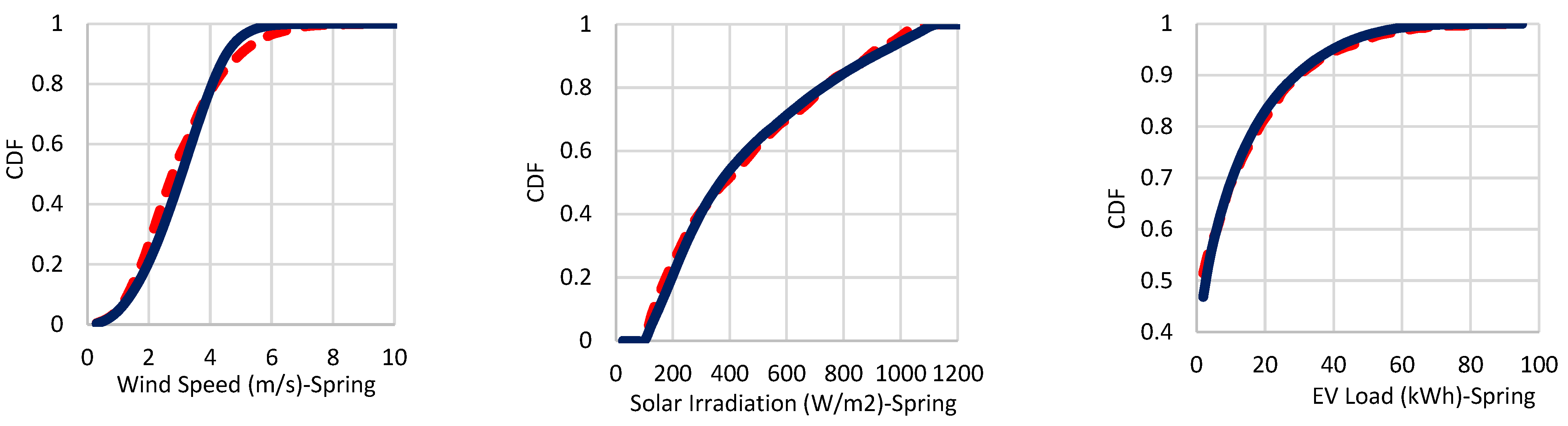
• A scenario generation approach based on GAN is developed to capture the uncertainties caused by wind speed, solar irradiation, EV load and the temporal correlation of these uncertain parameters. The method is designed to generate scenarios for each season to emulate stochastic generation and consumption.

The next section of this paper elaborates on the modelling of each component of the microgrid and describes the methodology. The corresponding formulation of the microgrid planning problem is presented in Section 3. Section 4 illustrates the numerical results extracted from the simulations. Eventually, the related conclusions are explained in the last section.

2. System Model and Methodology

In this paper, a stand-alone microgrid composed of PV generation systems, wind generation systems, and EV charging stations is studied. The system is supported by a battery energy storage system (BESS) composed of lithium-ion (Li-ion), lead acid (LA), and 2nd life Li-ion (SLi-ion) batteries. Figure 1 illustrates the system, which uses a common DC bus to connect the system components. In this framework, all batteries are connected to the coupling point by power electronic converters. In some types of research, such as [28], an idea is presented to connect the batteries directly without using converters. Nonetheless, the framework can be generalised to an AC system. In the following, the models used for each of these elements are explained. After the models are presented, the uncertainty modelling scheme is presented.

2.1. PV Generation Modelling

To model the power generated by PV panels, the irradiation received by PV panels has to be modelled initially. The irradiation that the PV uses to generate power is composed of three main elements as follows [29]:

$$G_{T,\beta }\left(t\right)=G_{B,\beta }(t)+G_{D,\beta }(t)+G_R(t)$$

(1)

In this relation, $G_{T,\beta }\left(t\right)$, is the global irradiance in ($\mathrm{W}/{\mathrm{m}}^2$), $G_{B,\beta }(t)$, $G_{D,\beta }(t)$, and $G_R(t)$ are the direct, diffuse, and reflected irradiation components for an inclined PV surface with the tilt angle of β in ($\mathrm{W}/{\mathrm{m}}^2$). After the global irradiance for the tilted surface is calculated, the total power generated by the PV generation system can be calculated as follows:

$$P_{PV}\left(t\right)=N_{PV}{\eta }_{PV}{A}_{PV}{G}_{T,\beta }\left(t\right)$$

(2)

where $A_{PV}$ and ${\eta }_{PV}$ are the solar panel area in (${\mathrm{m}}^2$) and solar power efficiency. $N_{PV}$ is the total number of PV panels.

2.2. Wind Generation Modelling

The output power generated by a wind turbine can be estimated as (3) [30].

$$P_W\left(t\right)=\left\{\begin{array}{c} 0 for v\left(t\right)\le v_{ci}\\ \begin{array}{c}a+b.V^w for v_{ci}\le v\left(t\right)\le v_R\\ \begin{array}{c} P_R for v_R\le v\left(t\right)\le v_{co}\\ 0 for v\left(t\right)\ge v_{co}\end{array}\end{array}\end{array}\right.$$

(3)

where:

$$a=P_R{v}_c/(v_{ci}-v_r)$$

(4)

$$b=P_R/(v_R-v_{ci})$$

(5)

power generated by the wind turbine in (kW). In addition, $v(t)$, $v_{ci}$, $v_R$, $v_{co}$, and $w$ show the wind speed, cut-in wind speed, rated wind speed, cut-out wind speed, and the Weibull factor, respectively. The Weibull factor specifies how the wind generation changes for wind speeds between the cut-in and rated wind speed. Usually, this factor is equal to 1, and a linear relation is assumed for this wind speed interval. In this research, the power-wind speed curve is available for the utilised wind turbines and is used to calculate the output power for each hour according to the related wind speed [31].

2.3. Battery Capacity Fading Model

Battery capacity fading is caused by two types of degradation: cycle degradation and calendar degradation. While the former is caused by the charge and discharge of the battery, the latter is related to the stored energy in the battery [32]. Cycle degradation has been regarded in several microgrid capacity sizing studies. However, in a number of these studies, for incomplete cycles, the degradation of complete cycles is calculated. Figure 2 shows an example of how the incomplete cycles are calculated using the rain-flow counting algorithm [33]. In this figure, the total cycle degradation is calculated using the following equation:

$$\begin{array}{c}Deg=AG\left(DOD=50\mathrm{\%}\right)+AG\left(DOD=40\mathrm{\%}\right)-AG\left(DOD=10\mathrm{\%}\right)+AG\left(DOD=50\mathrm{\%}\right)\\ -AG(DOD=20\mathrm{\%})\end{array}$$

(6)

In (6) $Deg$, and $AG\left(DOD=\mathrm{*}\right)$ indicate the total cycle degradation and the cycle degradation (complete cycle) for a depth of the discharge. It must be noted that if complete cycle degradation was applied for this figure, the calculated degradation would be the degradation of full cycles at points 2, 4, and 6, which would overestimate the amount of degradation for the battery. The cycle degradation for a specific depth of discharge $DOD$ is calculated as:

$$D^{Cyc}={\alpha }^{cyc}DOD{C}_{BESS}$$

(7)

where ${\alpha }^{cyc}$ is the percentage of capacity fading for 1000 cycles of 100% $DOD$. It can be illustrated that by simplifying (7), the relation (8) can be used instead [34].

$$D^{Cyc}={\alpha }^{cyc}{P}_{dis}\Delta t$$

(8)

Calendar ageing is proportional to the SOC of the battery and can be formulated as:

$$D^{cal}={\alpha }^{cal}{C}_{BESS}SOC$$

(9)

However, the corresponding coefficient ${\alpha }^{cal}$ shows the percentage of capacity fade for a certain amount of SOC that is stored for 1 month. To convert this capacity fading for each time interval $∆t$, (9) is used (30 days is assumed for a month with 24 h for each day). Instead of (9), the following relation can be used where $E$ shows the stored energy in the battery:

$$D^{cal}={\alpha }^{cal}E/(720∆t)$$

(10)

The total amount of degradation is obtained by the aggregation of two types of degradation for each time interval [34].

2.4. Uncertainty Modelling

The system uncertainties are caused by the stochastic generation of PV/wind and the stochastic EV loads. To manage the uncertainty of the system, various scenarios are generated according to the wind speed, total solar irradiation, and the EV load. In this research, generative adversarial networks (GAN) are used to generate the scenarios. In the past literature, various scenario-generating approaches have been applied for modelling the uncertain space, such as Monte Carlo Sampling (MCS) and Latin Hypercube Sampling (LHS) based on methods like copulas for modelling the distributions and correlations. Most of these approaches are based on fitting a probability density function (pdf) to a data set and randomly selecting data from this function. Nevertheless, the probability density functions are based on statistical assumptions which are not always valid for dynamic and time-varying uncertainties [18]. In this research, the probability density function for the EV charging station loads is not known. Furthermore, a specified pdf for the solar irradiation and wind speed cannot always be valid. Therefore, a data-driven approach is used for generating scenarios that do not require a probability distribution function and are able to capture the temporal correlations for various uncertain parameters, including the EV station charging load, solar irradiation, and wind speed. After the scenarios are generated, to compromise between the computational burden and the accuracy of the results, the number of scenarios is reduced using the k-means algorithm. Figure 3 shows an overview of the uncertainty management scheme. In the following sections, each of the stages is explained.

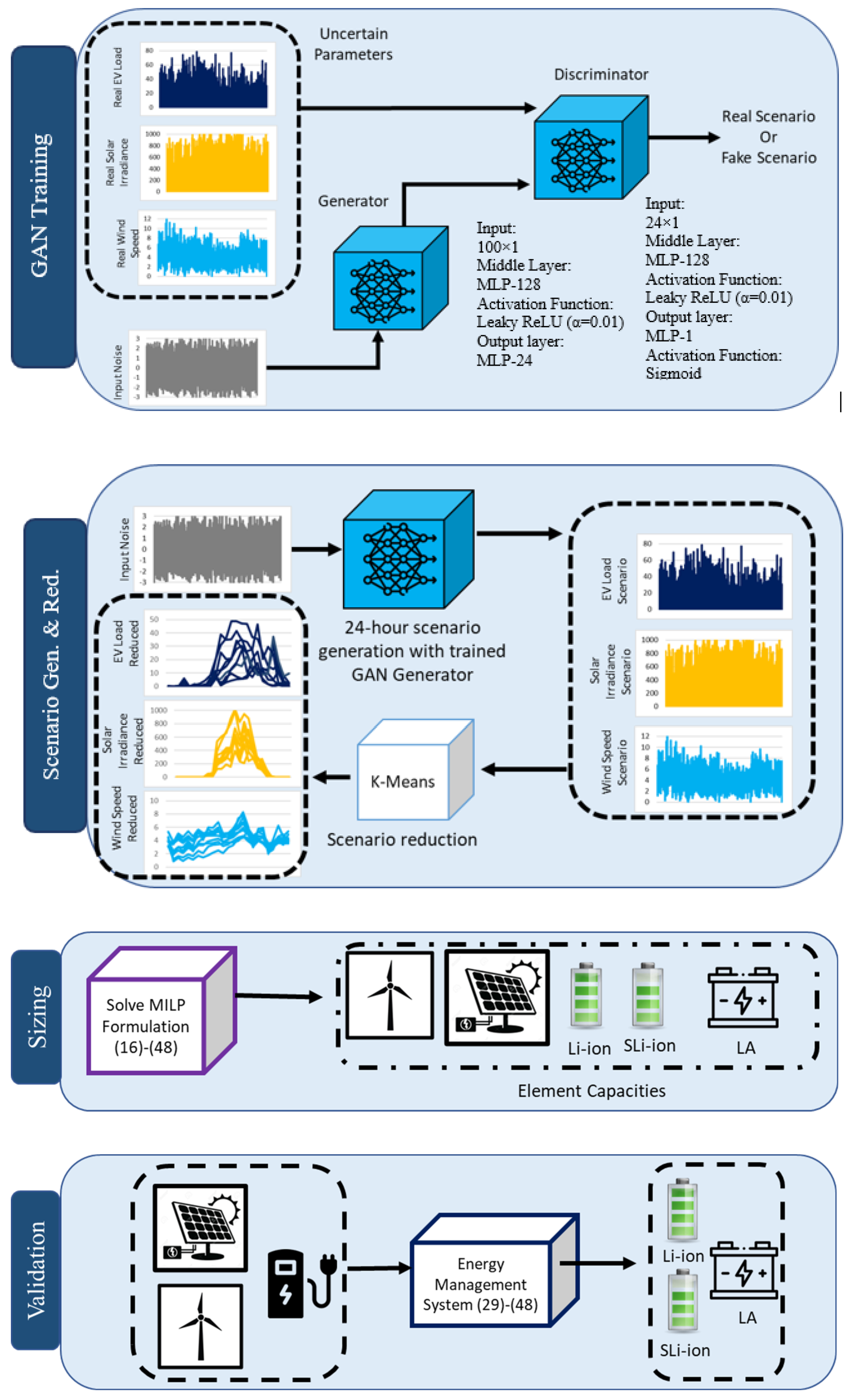
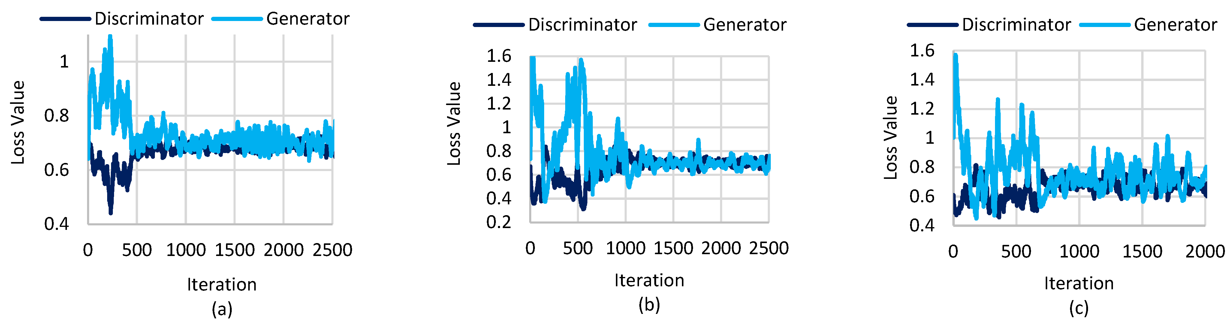
2.4.1. Scenario Generation

GAN is a type of machine-learning approach that can be used to emulate a set of data [35]. Without requiring information about the distribution of data (wind speed, solar irradiation, and EV load), GAN is able to generate scenarios from a noisy input. The idea of these networks is based on a MinMax game between two interconnected networks, which are recognised as the generator (G) and the discriminator (D), as shown in Figure 3. While the discriminator acts as a binary classifier and tries to detect the real data, the generator attempts to confuse the discriminator by generating fake data. The generator and discriminator compete until they reach the Nash-equilibrium point (Nash equilibrium is a situation where none of the players can increase their profit by changing their strategy while the strategy of other players is fixed). Eventually, after the generator is trained, it can be separated and used to generate scenarios with the noise input. The objective function of this system, in which the generator generates samples from the input noise ($z$) similar to real samples ($x$), can be formulated as follows:

$${Min}_{\theta }{Max}_{\omega }\left(E_{x~P(x)}\left[log\left(D_{\omega }(x)\right)\right]+E_{z~P(z)}\left[log\left(1-D_{\omega }\left(G_{\theta }\left(z\right)\right)\right)\right]\right)$$

(11)

In (11), $D_{\omega }$ and $G_{\theta }$ show the discriminator and generator which have the set of weights and biases $\omega$ and $\theta ,$ respectively. $P(x)$ is the real historical dataset from which the real samples $x$ are taken. $P(z)$ is the latent space (a random generator such as a noise function) that the random data $z$ is taken from. $E(.)$ is the expected value.

In each iteration, the generator and discriminator are trained concurrently. The general loss function from the view of the generator network is as follows:

$${Min}_G{L}_G\left(G\right)=-E_{z~P(z)}\left[log\left(D_{\omega }\left(G_{\theta }\left(z\right)\right)\right)\right]$$

(12)

The goal of the generator is to confuse the discriminator which is fulfilled by (12) [35]. When the generator is trained, all the parameters of the discriminator are fixed, and the weights and biases of the generator are updated by minimising (12). Also, the loss function from the view of the discriminator is as follows:

$${Max}_D{L}_D\left(D\right)=E_{x~P(x)}\left[log\left(D_{\omega }\left(x\right)\right)\right]+E_{z~P(z)}\left[1-log\left(G_{\theta }\left(z\right)\right)\right]$$

(13)

The discriminator’s objective function is to distinguish between the fake samples generated by the generator and the real samples by updating the weights and biases $\theta$ for each iteration. Like the previous step, the weights and biases of the generator are fixed for this update. For the initial iterations, the discriminator will be able to easily detect the fake samples, the discriminator loss function will be low, and the generator loss function will have a high value. However, after a number of iterations, the loss function of the discriminator and the generator will increase and decrease, respectively, and the discriminator will be fooled into recognising the true and fake samples. After the generator is trained, it can be used to generate scenarios. The training process can be fulfilled by using Algorithm 1 below.

Algorithm 1: Training of GAN for scenario generation

Default Values: Mini-Batch ($N_{bch})$, number of iterations ($N_{it}$) Initialise hyperparameters $\theta$ and $\omega$ for generator and discriminator

In Algorithm 1, the Adam (adaptive moment estimation) optimiser is used, which is based on estimating the first and second-order moments. In terms of computation and memory requirements, the optimiser is efficient for large-scale problems with many parameters and data [36].

It is worth mentioning that using a solo deep learning model, such as a convolutional neural network model, can make it difficult to generate scenarios. If the deep learning model is trained with the historical dataset, it will perform as a forecaster. Forecasted values have errors; however, their errors are usually low, and the outputs of a solo CNN can be very similar to realised profiles. By merely using CNNs, it is difficult to generate scenarios which are similar to the real parameter profiles. To generate these datasets, in addition to a generator which is fed by white noise (despite a CNN which is fed by real data), a discriminator is also required to assist the generator in learning how to generate data profiles which are similar to the real data and not detectable by the discriminating network as “fake” data. Also, in this research, in order to investigate hyperparameter tuning, different combinations of various hyperparameters such as the batch size (10 to 50 batches), epochs (1000 to 5000), optimiser (Adam, SGD, RMSprop), number of nodes, and number of layers are examined for the generator and discriminator. In addition to the mentioned optimisers, the AdamW optimiser can also be used for training the discriminator and generator by also considering the weight decay to be optimised.

In this study, for each season, a separate GAN is trained for the wind speed, solar irradiation, and EV load, as illustrated in Figure 3. After the GAN is trained, it is used to generate scenarios for each stochastic parameter and for each season. Eventually, using the k-means method, the generated scenarios are reduced to a set of scenarios which represent the total stochastic space.

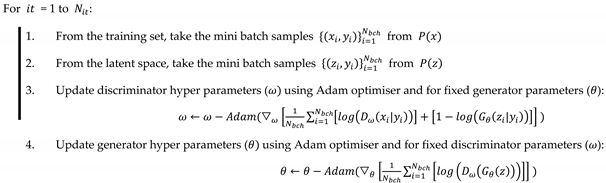
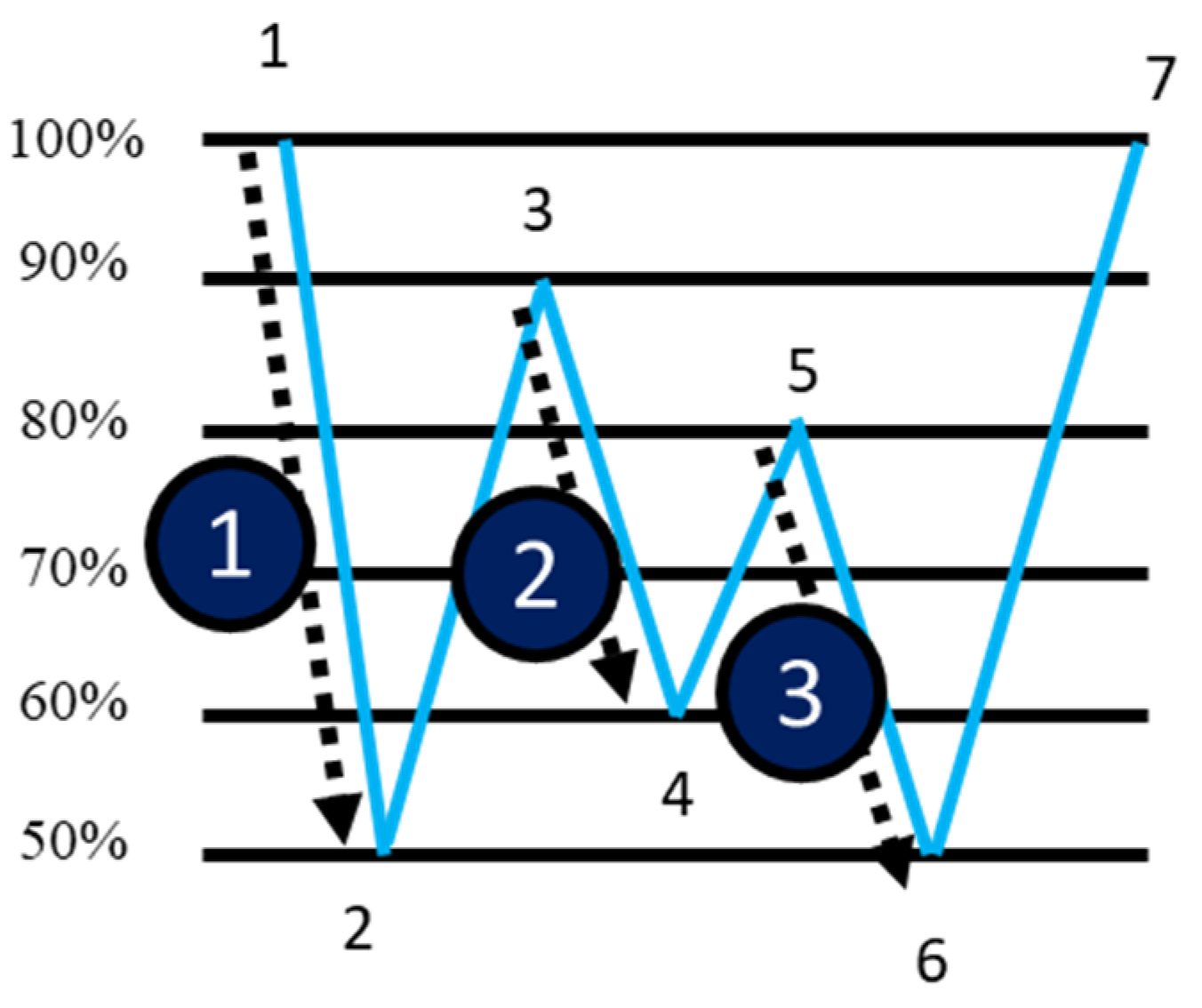
2.4.2. Scenario Reduction

In this section, after the scenarios are generated for the electric vehicle charging loads, solar irradiation, and wind speed, the scenarios are reduced using the k-means approach [37]. k-means is a clustering algorithm that specifies k clusters with the corresponding centres and specifies which data objects belong to which cluster. The k-means algorithm seeks to find the optimal centres of each cluster in order to minimise the distance of the centres from the data samples in the vicinity of these clusters. This distance is based on calculating the Euclidean distance between the samples as follows:

$$d\left(a^p,c^q\right)=\sqrt{\sum _{i=1}^n{\left(a_i^p-c_i^q\right)}^2}={‖a^p-c^q‖}_2$$

(14)

where $a$ and $c$ are sets of n-dimensional of data samples and cluster centroids, respectively. Also, $a_i^p$ and $c_i^q$ show the p^th sample from the data set and the q^th centroid of the clusters. The k-means algorithm is initiated by selecting k data sets as the cluster centres and by defining a loop; the centres are modified for each iteration. During each iteration, each data set is assigned to the closest centre according to the calculated Euclidean distance. In the next step, the centres are shifted to the mean of all data sets of a cluster. The calculation continues until the distance between the new and previous centres is below a specified amount as follows [37]:

$$\sum _{i=1}^k{‖c_t^i-c_{t-1}^i‖}^2\le ϵ$$

(15)

where $c_t^i$ and $c_{t-1}^i$ are the centroids of the ith cluster for the tth and tth−1 iteration. The clustering algorithm is illustrated in Algorithm 2 below:

Algorithm 2: k-means algorithm

Input:      Input data set: $\mathbf{A}=\left\{{\mathit{a}}^1,{\mathit{a}}^2,\cdots ,{\mathit{a}}^j\right\}, a^i\in R^n$  Output:      Output: Cluster Centroids: C$=\left\{{\mathit{c}}^1,{\mathit{c}}^2,\cdots ,{\mathit{c}}^{\mathit{k}}\right\},$ Data set of each cluster: D$=\left\{{\mathit{d}}^1,{\mathit{d}}^2,\cdots ,{\mathit{d}}^{\mathit{k}}\right\}$

Initialisation:      Select k random points from the dataset $\mathbf{A}$ as the centroids

While  ${\sum }_{i=1}^k{‖c_t^i-c_{t-1}^i‖}^2>ϵ$: For i = 1 to j:      ${argmin}_m{‖a^i-c^m‖}_2\to m^{*}$      $D^{m^{*}}\cup \left\{a^i\right\}\to D^{m^{*}}$ For i=1 to k:      $c^i={\displaystyle \frac{1}{\left|c^i\right|}}{\sum }_{a^j\in c^i}{a}^j$ Return:      C and D

2.4.3. Methodology

The overall diagram of the proposed microgrid planning method is presented in Figure 3. In the first step, the GAN is trained using the gathered data for EV load, wind speed, and solar irradiation, which are determined for each season (December, January, February for winter, March, April, May for spring, June, July, August for summer, and September, October, November for autumn). In the second stage, after the generative network is trained, it is used for generating various scenarios for 24 h, and the corresponding annual profiles are built based on these scenarios; however, to reduce the computational burden of the problem, the scenarios are reduced using k-means. After the final scenarios are selected, the MILP formulation is solved for each scenario, and the final capacities are acquired. Eventually, with the goal of assessing the results, the obtained capacities are passed to the energy management system, and the performance of the system in terms of the total unmet load and battery degradation is evaluated.

3. Microgrid Planning Formulation

3.1. Microgrid Capacity Sizing

The objective function of the problem is composed of the capital cost (CAPEX) and the operation and maintenance cost (OPEX) of each element as follows:

$$F(s)={Cost}_W\left(s\right)+{Cost}_{PV}\left(s\right)+\sum _{tc=1}^{N_{TC}}{Cost}_{BESS}\left(s,tc\right)+\sum _{tc=1}^{N_{TC}}{Cost}_{Conv.}\left(s,tc\right)-\sum _{tc=1}^{N_{TC}}{Sal}_{BESS}\left(s,tc\right)$$

(16)

$${Cost}_W(s)={CAPEX}_W{C}_W(s)+{OPEX}_W(s)$$

(17)

$${Cost}_{PV}(s)={CAPEX}_{PV}{C}_{PV}(s)+{OPEX}_{PV}(s)$$

(18)

$${Cost}_{BESS}(s,tc)={CAPEX}_{BESS}(tc)C_{BESS}(s,tc)+{OPEX}_{BESS}(s,tc)$$

(19)

$${Cost}_{Conv}(s,tc)={CAPEX}_{Conv.}(tc)C_{BESS}(s,tc)$$

(20)

$${OPEX}_W(s)=\sum _{y=1}^{N_Y}\sum _{t=1}^{N_T}{\displaystyle \frac{1}{{\left(1+r\right)}^y}}({OPEX}_{W,F}{N}_W(s)+{OPEX}_{W,V}{C}_W(s)Wind(s,t,y)∆t)$$

(21)

$${OPEX}_{PV}(s)=\sum _{y=1}^{N_Y}\sum _{t=1}^{N_T}{\displaystyle \frac{1}{{\left(1+r\right)}^y}}({OPEX}_{PV,F}{C}_{PV}(s)+{OPEX}_{PV,V}{C}_{PV}(s)PV(s,t,y)∆t)$$

(22)

$$\begin{array}{c}{OPEX}_{BESS}(s,tc)={\displaystyle \sum _{y=1}^{N_Y}}{\displaystyle \sum _{t=1}^{N_T}}{\displaystyle \frac{1}{{\left(1+r\right)}^y}}({OPEX}_{BESS,F}(tc)C_{conv}(s,tc)+{OPEX}_{BESS,V}(tc)(P_{ch}(s,tc,t,y)\\ +P_{dis}(s,tc,t,y))∆t)\end{array}$$

(23)

$${Sal}_{BESS}\left(s,tc\right)={\displaystyle \frac{\gamma .{CAPEX}_{BESS}(tc)}{{\left(1+r\right)}^{N_Y}}}\left(\left(1-EOL\left(tc\right)\right)C_{BESS}\left(s,tc\right)-\sum _{y=1}^{N_Y}\sum _{t=1}^{N_T}D\left(s,tc,t,y\right)\right)$$

(24)

$$C_W(s)=N_w{(s)PR}_W$$

(25)

$$C_{PV}(s)=N_{PV}(s){PR}_{PV}$$

(26)

$$C_{BESS}(s)=N_{BESS}{(s)PR}_{BESS}$$

(27)

$$C_{Conv}(s)=N_{Conv}(s){PR}_{Conv.}$$

(28)

In these relations, (17)–(20) show the total cost for each element of the microgrid including the wind turbine, PV panels, BESSs for different technologies and the converters for each BESS. The OPEX of each component of the microgrid is also indicated in (21)–(23) for the wind turbine, PV panels, and different technologies of the BESSs (there was no data for the OPEX of converters; however, if the OPEX of converters is available, it can be involved in the objective function). In (24), the residual value of the battery at the end of the planning horizon is calculated. In this relation, the residual capacity (obtained from subtracting the amount of capacity fade from the initial useable capacity) is multiplied by an initial percentage of the battery’s price. For these relations, the term $\left(1/{\left(1+r\right)}^y\right)$ is used for converting the costs in the later years to the present value according to the discount rate of $r.$ Relations (25)–(28) calculate the capacity from the number of elements used and the size of each unit element.

The objective function is restricted by the following constraints:

$$C_W(s)\le C_{W,max}$$

(29)

$$C_{PV}(s)\le C_{PV,max}$$

(30)

$$C_{BESS}(s,tc)\le C_{BESS,max}(tc)$$

(31)

$$C_{Conv}(s,tc)\le C_{Conv,max}(tc)$$

(32)

In (29)–(32), the capacity for each scenario for wind, PV, BESS, and converters are restricted to an upper bound. The load balance equation for the microgrid is as follows:

$$\begin{array}{c}{N}_{W}WG\left(s,t,y\right)∆t+C_{PV}PVG\left(s,t,y\right)∆t+{\sum }_{tc=1}^{N_{tc}}{P}_{dis,tc}(s,tc,t,y)+UL\left(s,t,y\right)=EV\left(s,t,y\right)+\\ {\sum }_{tc=1}^{N_{tc}}{P}_{ch,tc}\left(s,tc,t,y\right)+RS(s,t,y)\end{array}$$

(33)

In this relation, for each time interval for each year and of each scenario, the sum of the energy generated by the wind and PV systems in addition to the discharge of all batteries and the amount of load that is not supplied must provide the load, charge the battery, or be curtailed. The relations for the BES systems are as follows:

$$P_{ch}(s,tc,t,y)\le C_{conv}(s,tc)$$

(34)

$$P_{dis}(s,tc,t,y)\le C_{conv}(s,tc)$$

(35)

$$P_{ch}(s,tc,t,y)\le M{u}_{ch}(s,tc,t,y)$$

(36)

$$P_{dis}(s,tc,t,y)\le M{u}_{dis}(s,tc,t,y)$$

(37)

$$u_{ch}\left(s,tc,t,y\right)+u_{dis}(s,tc,t,y)\le 1$$

(38)

$$\begin{array}{c}{E}_{tc}\left(s,tc,t,y\right)=E_{tc}\left(s,tc,t-1,y\right)+\left({\eta }_{ch}(tc){\eta }_{Conv}(tc)P_{ch,tc}(s,tc,t,y)∆t\right)\\ -(P_{dis,tc}(s,tc,t,y)∆t/{\eta }_{dis}(tc){\eta }_{Conv}(tc))\end{array}$$

(39)

$${SOC}_{min}(tc)C_{BESS}(s,tc)\le E(s,tc,t,y)\le {SOC}_{max}(tc)C_{BESS}(s,tc)$$

(40)

$$RS\left(s,t,y\right)\le M(1-u_{dis}(s,tc,t,y)$$

(41)

$$UL\left(s,t,y\right)\le M(1-u_{ch}(s,tc,t,y)$$

(42)

In (34) and (35), the power discharged, and charged by the BESS are limited by the converter size and for each type of technology. Binary variables in (36)–(38) determine the charge and discharge states for the batteries. In these relations, M is any large value which is used for linearisation in MILP problems. The energy balance equation for each type of battery technology is demonstrated in (39). The energy stored in the batteries is limited by (40). Relations (41) and (42) show that if any battery is discharging, there should be no renewable energy spillage, and conversely, if there is any unmet load for a specific time interval, none of the batteries are permitted to charge. The degradation limitations of the batteries are as follows:

$$D^{cyc}\left(s,tc,t,y\right)={{\alpha }^{cyc}(tc)P}_{dis}(s,tc,t,y)∆t$$

(43)

$$D^{cal}\left(s,tc,t,y\right)={\alpha }^{cal}(tc)/(24\times 30)E_{tc}(s,tc,t,y)$$

(44)

$$D(s,tc,t,y)=D^{cyc}\left(s,tc,t,y\right)+D^{cal}\left(s,tc,t,y\right)$$

(45)

$$\sum _{y=1}^{N_Y}\sum _{t=1}^{N_T}D\left(s,tc,t,y\right)\le \left(1-EOL\left(tc\right)\right)C_{BESS}(s,tc)$$

(46)

Relations (43)–(45) calculate the amount of cycle degradation, calendar degradation, and total degradation for each type of battery, respectively. Equation (46) restricts the total amount of degradation to less than the end-of-life capacity fade of the battery for each type of technology. Eventually, the reliability constraints for the microgrid capacity sizing framework are as follows:

$$EENS\left(s,y\right)={\sum }_{t=1}^{N_T}UL(s,t,y)$$

(47)

$$EENS\left(s,y\right)\le {EENS}_{max}·\sum _{t=1}^{N_T}EV(s,t,y)$$

(48)

In (47), the total expected energy not supplied is calculated for each year of each scenario. Relation (48) limits this value to a maximum portion of the total EV load by ${EENS}_{max}$ (${0\le EENS}_{max}\le 1$).

When the capacities are obtained for each scenario, the final solutions are specified as the expectation of the capacities for all scenarios. The next section explains how these capacities are evaluated by the energy management system.

For the microgrid capacity planning section, the coefficient costs (CAPX, fixed OPEX, and variable OPEX) for various parameters used in the objective function are shown in

Table 2. Cost parameters for each component of the microgrid.

Component	CAPEX (£/kW)	Fixed OPEX (£/kW/Year)	Variable OPEX (£/kWh)
Wind	5000	83	0.016
PV	730	50	0.008
Li-ion Battery	335	8	0.00024
LA Battery	80	8	0.00024
SLi-ion Battery	150	8	0.00024
Converter	90	-	-

[34]. In addition, the battery characteristics are illustrated in

Table 3. Battery characteristics for each type of battery [34].

Parameter	Li-Ion	LA	SLi-Ion
${\eta }_{ch,tc}-{\eta }_{dis,tc}$ (%)	97–97%	90–90%	97–97%
${SOC}_{min}$ (%)	20%	50%	20%
${SOC}_{max}$ (%)	100%	100%	80%
${\alpha }^{cyc }$(per 1000 cycle) (%)	4.5%	61.5%	4.5%
${\alpha }^{cal }$(per month) (%)	0.125	0.125	0.125
EOL (%)	60	70	60

.

3.2. Capacity Sizing Assessment with the Energy Management System

After specifying the capacity of each component of the microgrid, the results are studied to quantify the efficacy of the proposed framework. To do so, an energy management scheme that minimises the unmet load (expected energy not supplied) is solved, considering the relations (29)–(48). The criteria for evaluating the results are based on the amount of unmet load and the total degradation of the batteries.

4. Simulations and Results

In this section, the results are presented to demonstrate the efficacy of the proposed capacity sizing scheme. For the scenario generation section, the Keras [38] library in Python is used to train the GAN networks (Keras is an open-source library that provides a Python interface for artificial neural networks). The details of the GAN used for generating scenarios for wind speed, solar irradiation, and EV load scenarios are illustrated in Figure 3, training stage.

In this research, an initial state of health (SOH) of 80% is assumed for the SLi-ion batteries. Also, the converter efficiency for all battery types is assumed to be 97%. The global irradiance and wind speed (10 m height) are extracted from [39] according to the coordination of the installation site. Finally, the data used for the EV load is extracted from the EV charging points of the Perth and Kinross Council [40]. The main limitation of this research is that it has not been able to access the EV charging profile for more than two years. By possessing access to larger EV charging datasets, more precise scenarios can be generated, and the microgrid capacity sizing can be conducted with a higher accuracy. The MILP problem is also formulated in the Python environment using the Spyder IDE [41] and the GUROBI solver [42] to solve it using a Core i7, 2.1 GHz PC with 16 GB RAM and setting the duality gap to 0%. Also, to reduce the number of scenarios using k-means and to initialise the clusters’ centroids, the k-means++ option can be used in Scikit-learn to obtain more effective results [43].

Two main study cases are investigated for the microgrid capacity sizing approach. In the first case, the capacity sizing is fulfilled by using a single technology, BESS. In the second case study, hybrid BESS technologies are studied for microgrid planning. For these studies, initially, 9000 scenarios are generated for the daily wind speed, solar irradiation, and EV load and for each season (as these scenarios are for 24 h and they are used for making 1 year EV charging load, solar irradiation, and wind speed profiles; an adequate number of scenarios have to be generated). By using k-means, the number of scenarios is reduced to 10 for each year (the number of reduced scenarios can be specified by the elbow method [44]). Figure 4 shows the loss function for the generator and discriminator for winter for the three uncertain parameters. The results indicate that for the first initial iterations, the discriminator is able to detect between the real samples, and the generator is not able to confuse the discriminator; however, after a few iterations, the generator starts generating samples that are similar to the real samples and the discriminator is not able to distinguish them.

To show the similarity of the generated scenarios to the real data from the statistical point of view, the cumulative distribution functions for the uncertain parameters are shown in Figure 5. The results verify that the generated scenarios are able to emulate the set of real data for wind speed, solar irradiation, and EV load. In addition, a comparison is made between the normalised values of some samples from the real dataset and the generated dataset for the solar irradiance, wind speed and EV load using the Euclidean distance to find similar samples in Figure 5. To show the similarity between these datasets in terms of correlation, the autocorrelation between these samples for each time lag is also shown in Figure 6. In the next section, the results of the microgrid capacity planning are presented for the two different case studies.

4.1. Single BESS Technology Use

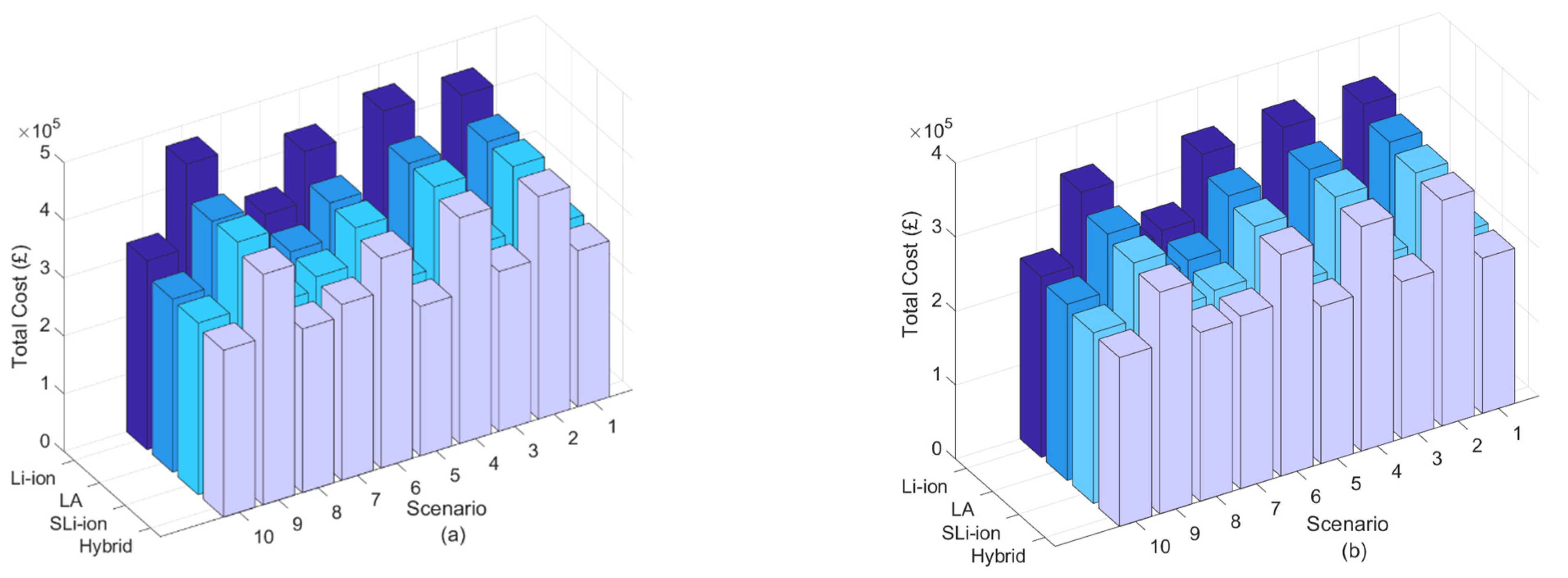
In this part, the simulation results are scrutinised for the utilisation of single technology types of battery.

Table 4. Microgrid planning cost for various study cases and EENS = 0.

BESS Type	Scenario#1 Cost (£)	Scenario#2 Cost (£)	Scenario#3 Cost (£)	Scenario#4 Cost (£)	Scenario#5 Cost (£)	Scenario#6 Cost (£)	Scenario#7 Cost (£)	Scenario#8 Cost (£)	Scenario#9 Cost (£)	Scenario#10 Cost (£)
Li-ion	371,433	559,212	438,444	606,928	362,084	540,559	480,344	423,876	774,297	417,563
LA	358,098	473,140	416,131	496,903	325,166	447,650	448,255	361,067	702,401	367,656
SLi-ion	352,144	478,819	406,921	510,220	325,681	457,867	452,566	363,209	689,997	371,382
Hybrid	347,909	452,658	397,476	479,286	314,873	430,677	444,727	344,331	674,013	354,413

compares the total capacity sizing cost for using each of these types of battery for the maximum level of reliability (${EENS}_{max}=0$). As expected, the new Li-ion batteries have the highest planning cost compared to LA and second-life Li-ion-batteries. In this study, scenario 9 has the highest planning cost with £774,297, £702,401, and £689,997 for Li-ion, LA, and SLi-ion batteries, respectively for the ${EENS}_{max}=0$ study case. For supplying 99% of the EV charging load, these costs decrease to £472,600, £412,868, and £415,861, and for 95% of the met load for each year, these values drop to £341,325, 316,066, and £308,104 for the three mentioned technologies, respectively.

The results indicate that the system planning cost can be decreased at the expense of a lower reliability level of charging EVs. Moreover, due to the high price of Li-ion batteries, the usage of these technologies results in high planning costs, even though they have a better degradation characteristic compared to LA and SLi-ion batteries. Figure 7 shows the planning cost for the other two reliability limits of ${EENS}_{max}=1\mathrm{\%}$ and ${EENS}_{max}=5\mathrm{\%}$. Although the study case of ${EENS}_{max}=0$, wherein a number of cases using LA batteries leads to lower planning costs, for the two other reliability levels, the planning cost is higher for LA batteries compared to SLi-ion BESS.

The size of each component for each scenario is presented in Figure 8 for ${EENS}_{max}=0$. This figure illustrates that for scenario 9, the optimiser sizes near 300 kW PV for all various battery technologies. However, for the other scenarios, the PV size is less than 100 kW due to a lower peak of EV charging load. For the wind generation capacity, scenario S7 has the largest size at 55.8 kW. The wind generation capacity is almost the same for different types of batterie for most scenarios. For battery sizing, the LA battery has larger capacities for all scenarios than Li-ion and SLi-ion. The reason for this solution is that despite Li-ion and SLi-ion batteries that can be discharged to a SOC of 20%, the LA batteries are only discharged to half of their capacity. In addition, the cycle ageing coefficient is larger for LA batteries compared to Li-ion and SLi-ion, which results in a larger capacity to compensate for the battery capacity loss caused by cycling.

The same interpretation can be provided when comparing the sizes of Li-ion and SLi-ion batteries. The SLi-ion can be charged up to 80% of the specified capacity. Hence, when compared to a fresh Li-ion battery with the same conditions, the capacity of the SLi-ion battery has to be increased to achieve the same capability as a fresh Li-ion battery. The other reason for the selection of larger sizes of SLi-ion compared to Li-ion batteries is the cheaper price. In a number of scenarios, for example, for scenario S2, the optimiser decreases the capacity of wind generation (14.4 kW) and tries to manage the load with a lower cost by increasing the size of SLi-ion batteries. For the converters, in most of the scenarios, the optimisation sizes have similar capacities for these components independent of the type of battery that is used.

To investigate the effect of the system reliability of the microgrid component sizes,

Table 5. Average microgrid component sizes for all scenarios and all battery-type study cases.

Reliability Level	PV (kW)	Wind (kW)	Battery (kWh)	Converter (kW)
${EENS}_{max}$ = 0	65	6.3 × 6.2	887	73
${EENS}_{max}$ = 1%	60.3	4.7 × 6.2	620	56
${EENS}_{max}$ = 5%	64.4	3.3 × 6.2	393	42

shows the average size of all scenarios and for all battery-type study cases for three levels of reliability. As it was expected, when higher reliability levels are desired, the overall component size increases. For instance, for the single SLi-ion study case, the capacity size of the battery is 624 kWh and 194 kWh for ${EENS}_{max}=0$ and ${EENS}_{max}=5\mathrm{\%}$ respectively. For the wind turbines and for the two mentioned levels of reliability, the wind capacity sized for the single SLi-ion study case is 7 × 6.2 kW and 4 × 6.2 kW, respectively.

4.2. Hybrid BESS

In this section, the results of using hybrid BESS technologies for microgrid capacity sizing are presented. The numerical values of the planning cost for this study case are presented in Table 4 for the case of ${EENS}_{max}=0$ and compared with the planning costs of using single types of BESS technology. For the hybrid BESS study case, the three types of batterie, including Li-ion, LA, and SLi-ion, are considered in the optimisation problem. The table shows the lower microgrid planning cost when using hybrid BESS technologies. The results show that using new Li-ion batteries only leads to expensive plans for all scenarios. For instance, when using hybrid BESS technologies, for scenario 9, the planning cost is £100,284 cheaper. In addition, compared to the single usage of LA and SLi-ion batteries, hybrid BESS planning leads to lower system costs. It is worth mentioning that for the hybrid BESS planning studies, the optimiser does not include any Li-ion battery capacity for any scenario. The reason for this strategy is the high cost of using this type of battery for the system, and for all scenarios, a combination of LA and SLi-ion is used. Utilising hybrid BESS technologies also results in lower planning costs for lower reliability levels. Figure 9 shows the capacity of each component for each scenario and each reliability level. Like the single BESS technology study case, for most of the components and scenarios, the capacity decreases when higher levels of ${EENS}_{max}$ is acceptable.

The advantage of using hybrid BESS technologies in the microgrid is not limited to the lower cost of the system. Deferring the LA battery replacement is the other benefit of hybrid BESS usage.

Table 6. Average capacity fades (kWh and % of total capacity) for LA and Li-ion batteries using single and hybrid BESS technology for microgrid capacity planning.

	${\mathit{E}\mathit{E}\mathit{N}\mathit{S}}_{\mathit{m}\mathit{a}\mathit{x}}$ = 0		${\mathit{E}\mathit{E}\mathit{N}\mathit{S}}_{\mathit{m}\mathit{a}\mathit{x}}$ = 1%		${\mathit{E}\mathit{E}\mathit{N}\mathit{S}}_{\mathit{m}\mathit{a}\mathit{x}}$ = 5%
	Single	Hybrid	Single	Hybrid	Single	Hybrid
LA Degradation	170 kWh—12.7%	88 kWh—8.5%	152 kWh—15.2%	60 kWh—9.1%	123.2 kWh—19.3%	33 kWh—9.6%
SLi-ion Degradation	29 kWh—4%	11.72 kWh—6.08%	22.8 kWh—4.4%	12 kWh—6.8%	16 kWh—5.3%	11 kWh—7.5%

shows the average of degradation for the LA and SLi-ion batteries for the two study cases of using single and hybrid BESS technologies and for the 10 years planning horizon. As the results indicate, not only has the battery degradation decreased for the LA battery and for the hybrid BESS technology utilisation, but the percentage of battery capacity fade has also been reduced compared to the case of only using the LA battery.

Also, for the SLi-ion battery, although the percentage of capacity fade increases, the amount of battery degradation decreases when a hybrid BESS technology is considered for the planning. Figure 10 shows the charge and discharge power of the LA and SLi-ion batteries for the last scenario and the last year of operation with ${EENS}_{max}=0$. This figure illustrates that in the hybrid BESS usage case, the LA is discharged only for high levels of EV charging load, which decreases battery degradation. It should be noted that the model is able to consider other types of battery chemistries with the related data and costs indicated in Table 3.

To show the sensitivity of the results to the prices, another case study is presented for the microgrid capacity sizing problem. For this case, a hybrid battery energy storage capacity sizing with an ${EENS}_{max}=0$ is studied, and the CAPEX of Li-ion batteries are decreased to 200 £/kWh with the same prices for the two other batteries. The results of this study case are presented in

Table 7. Results for the sensitivity of results to the Li-ion battery price.

Scenario	Total Cost (£)	PV (kW)	Wind (kW)	Li-ion (kWh)	LA (kWh)
#1	346,155	102	4 × 6.2	109	500
#2	448,986	55	6 × 6.2	272	1230
#3	395,758	35	8 × 6.2	101	424
#4	476,281	11	8 × 6.2	209	1534
#5	313,068	21	6 × 6.2	109	506
#6	427,170	33	6 × 6.2	269	1306
#7	443,391	33	9 × 6.2	89	588
#8	341,802	29	5 × 6.2	197	1043
#9	669,309	327	2 × 6.2	365	949
#10	352,700	20	6 × 6.2	105	1089

. As can be seen from this table, the optimiser does not size any SLi-ion batteries. Instead of this type of battery, the optimiser sizes Li-ion batteries as the price difference with the SLi-ion battery type is decreased. For this case study, not only are Li-ion batteries sized, but the total planning cost is also decreased compared to the case in which the Li-ion battery CAPEX is 335 £/kWh.

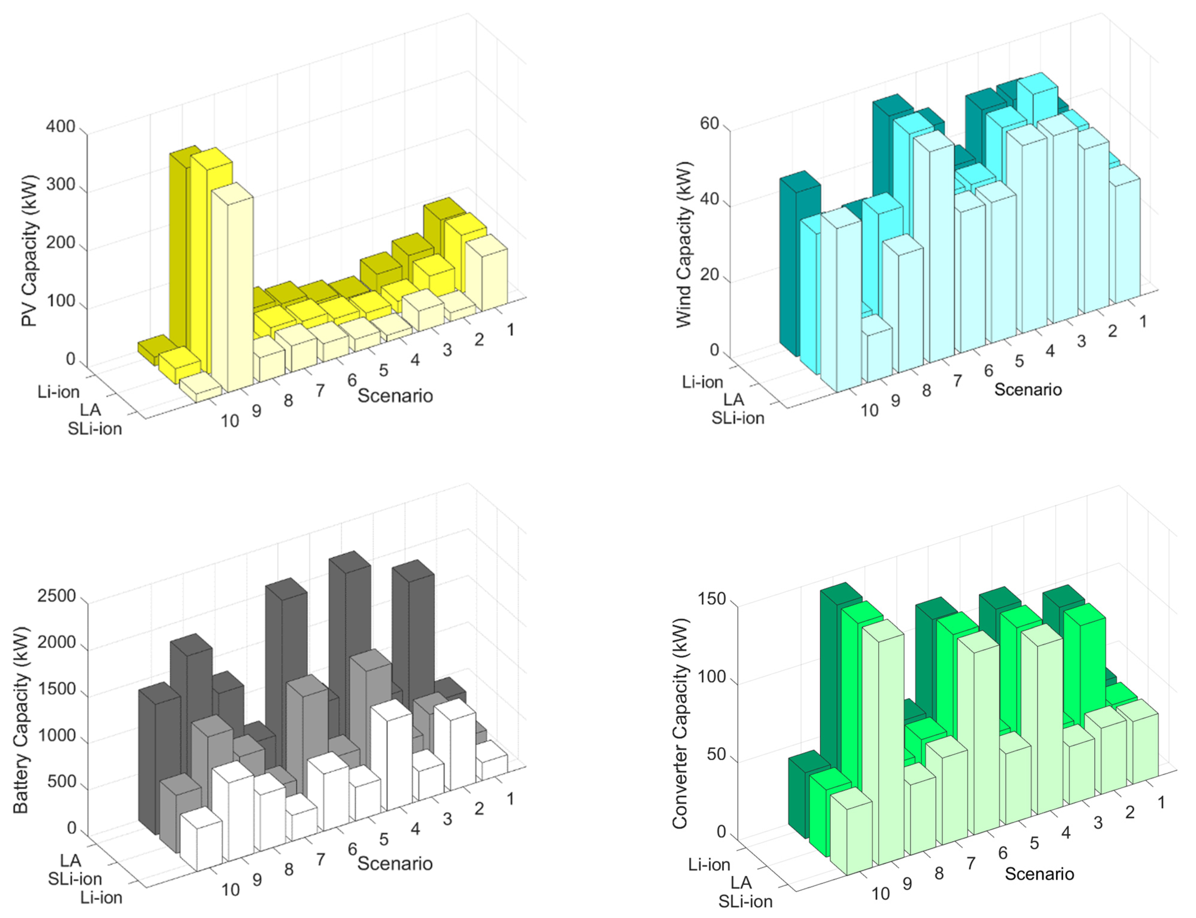
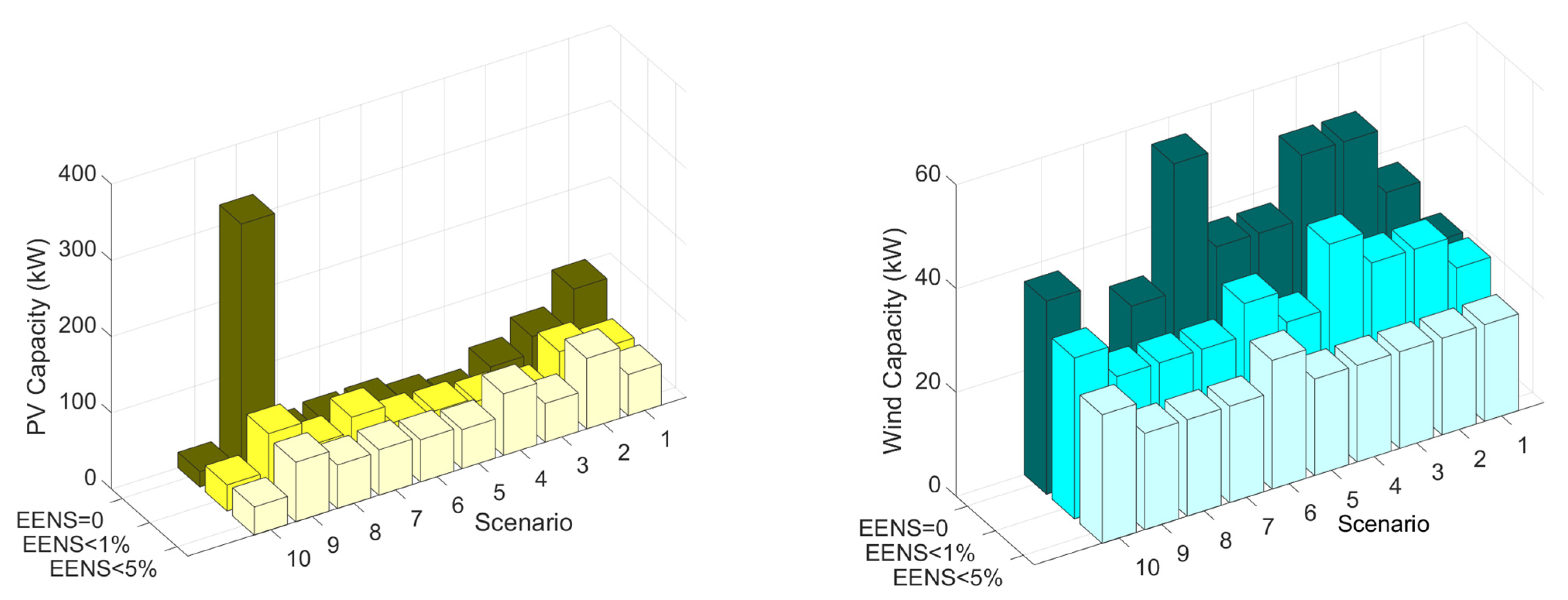
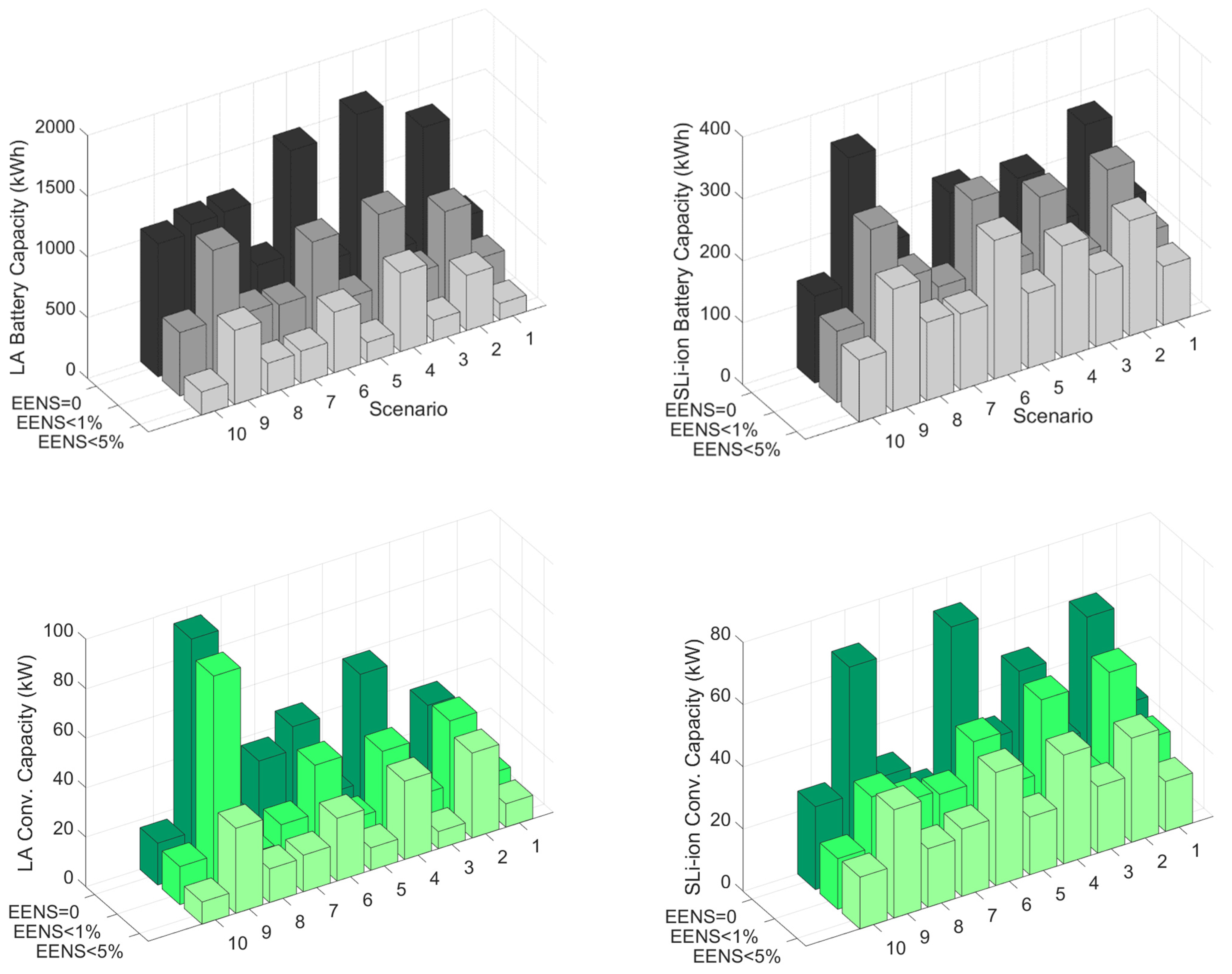
4.3. Capacity Evaluation

In this section, the performance of the capacities determined in Section 4.2 is evaluated using the energy management formulation. For this assessment, 50 new scenarios are generated, and the results are assessed in terms of the total unmet load for 10 years for all types of batteries.

Table 8. Summary of results for EMS study with 50 scenarios.

Battery Type	PV (kW)	Wind (kW)	BESS (kWh)	Conv. (kW)	Total Plan Cost (£)	EENS (%)
Li-ion	67.4	7 × 6.2	540	73	446,672	0.64
LA	69.7	7 × 6.2	1330	73	373,851	0.5
SLi-ion	67	7 × 6.2	792	73	371,962	0.54
Hybrid	67	6 × 6.2	1033LA- 261SLi-ion	31 LA- 42 SLi-ion	357,270	0.49

shows the size of each component, the total planning cost and the expected unmet load for these scenarios. As it was expected, the HBESS study case has the least planning cost. In addition, compared to the Li-ion, LA and SLi-ion single utilisation, the HBESS study case has a lower expectation for the amount of unmet load.

To show the robustness of the obtained capacities, the obtained capacities for the hybrid battery energy storage system are used for the energy management system (EMS), assuming a 10% decrease for wind generation, a 10% decrease for the PV generation, and a 10% increase for the EV charging load. Indeed, this case study shows how robust the results are against exacerbated situations in terms of renewable generation decrease and EV charging load increase. To do so, the EMS is executed for another 10 new scenarios; the results of this study (expected value of all scenarios) are shown in

Table 9. Results for robustness study of the obtained capacities for the HBESS Planning.

Study Cases	EENS (%)	LA Degradation (%)	Li-Ion Degradation (%)
Base Case	0.36%	9.5%	5.5%
10% Wind Generation decrease	0.43%	9.7%	5.7%
10% PV Generation decrease	0.41%	9.7%	5.7%
10% EV charging increase	0.71%	10.3%	6%

. The results show that even for an exacerbated condition of wind or PV generation (10% decrease), the system is still able to supply the load with a high-reliability level, and the unmet load will be less than 1%. In addition, there is a trivial change in battery degradation. For the EV charging load of a 10% increase, also the system is robust, and the load is supplied with an unmet load of less than 1%.

5. Conclusive Remarks, Discussions, and Future Work

5.1. Conclusive Remarks

In this paper, a scenario-based capacity planning model incorporating hybrid battery energy storage technologies is presented for a renewable-based microgrid to supply EV charging stations. In addition, generative adversarial networks (GAN) are used for generating scenarios which are similar to the real behaviour of wind speed, global horizontal irradiation and EV charging load of the stations and the number of scenarios is reduced by using the k-means algorithm. Three various battery types, including lithium-ion, lead acid, and second-life lithium-ion batteries, are considered.

The generated scenarios for wind speed, solar irradiation, and the EV load are able to emulate the behaviour of the real dataset in terms of statistic values and temporal correlation between different hours. For the capacity planning stage, the results demonstrate that the usage of hybrid BESS technologies results in lower costs for various reliability levels. The Hybrid utilisation case has the maximum cost reduction of 21%, 4.6%, and 6% compared to the case where only Li-ion, LA, and SLi-ion batteries are used. The other advantage of using a hybrid BESS system is decreasing the capacity fading of the LA batteries and postponing the need to replace them. For the reliability levels of ${EENS}_{max}=0$, ${EENS}_{max}=1\%$, and ${EENS}_{max}=5\%$, the LA battery capacity fading decreases 4.2%, 6.1%, and 9.7% respectively.

For the energy management system, the expected capacity of each component of all scenarios is considered as the designated size for that element and the energy management system is executed for 50 new scenarios. The results indicate that the unmet load for the hybrid BESS is 0.49%, which has a better performance than the LA and SLi-ion batteries, which have 0.5% and 0.54% of unmet load over a 10 years period. Only the new Li-ion battery has better performance, with a total unmet load of 0.25%. However, using a single Li-ion BESS technology comes up with a plan which is 25% more expensive than using the hybrid BESS composed of LA and SLi-ion batteries.

5.2. Discussions

A hybrid BESS microgrid has remarkable financial and environmental impacts. From the point of view of finance, by decreasing the planning cost of off-grid microgrids, the projects will be more profitable, and it can absorb more investments for establishing EV charging stations supplied by off-grid microgrids. This also alleviates the load burden of charging EVs on electrical grids and removes the necessity of investing in upgrading the equipment capacity of power networks.

From the environmental point of view, the hybrid battery system reduces the need for battery replacement and disposal, which can lead to environmental damage caused by the leak of toxic chemicals in the soil and groundwater if they are not recycled properly. In addition, growing interest in using HBESS will help reduce dependency on fossil fuel generation, which will reduce greenhouse gas emissions and enhance the environmental aspects of power generation systems.

The practical implementation of off-grid microgrids supplying electric vehicles can be challenging and restricting. The first limitation of these systems is the site location. The equipment used in these systems, such as the PV panels and wind turbines, usually needs more space than fossil fuel-distributed generation units. Hence, finding appropriate sites with sufficient solar irradiation and wind speed where this equipment can be installed is challenging, especially in city centres and suburbs. Social and cultural aspects can also be challenges for the establishment of off-grid microgrids. Local communities can be reluctant to accept this type of technology and may try to prevent their construction. Renewable generation intermittency is another practical challenge for the system. Although renewable generation is supported by the HBESS, and the design is robust against solar irradiation and wind speed, the reliability of the system can still be diminished. Hence, a proper energy management system (EMS) with a strong forecasting system is required to obtain maximum reliability for the system. Economic challenges for supplying EV charging stations with off-grid microgrids should also be considered. These systems have high upfront investments, and the financial resources required for these projects are limited.

5.3. Future Work

Future research could be conducted on incorporating other BESS technologies, such as Sodium-Sulfur (NaS) and vanadium redox flow batteries (VRFB) batteries for hybrid BESS capacity sizing for microgrids. Sodium-Sulfur (NaS) has the advantage of providing high power responses. For applications with a short duration, these types of technology can supply up to five times their nominal power [45]. It also has low maintenance costs and low self-discharge rates. Nevertheless, this type of technology needs high operation temperatures, which can be challenging to deal with [46]. The other disadvantage of these types of batteries is the low round-trip efficiency. While the round-trip efficiency for Li-ion and LA batteries is between 80–90%, the efficiency of Sodium Sulfur is 75%. The higher CAPEX of these batteries is another drawback compared to Li-ion and LA batteries.

Vanadium redox flow batteries (VRFB) are another type of battery which can be considered for stationary applications. These types of batteries have long lifetimes and are less vulnerable to high DODs [45]. Hence, they will have less capacity fading. The main flaw of these batteries is their lower round-trip efficiency (75–85%) and large sizes.

The voltage-SOC characteristic behaviours of batteries can be considered for optimal hybrid BESS capacity sizing for microgrids. If the batteries are connected directly to each other without power electronics interfaces, the voltage-SOC curve of each type of battery affects the performance of each battery in terms of the amount of power charge or discharge. This can also be investigated for future research.

References

1. Dong, F.; Zhu, J.; Li, Y.; Chen, Y.; Gao, Y.; Hu, M.; Qin, C.; Sun, J. How green technology innovation affects carbon emission efficiency: Evidence from developed countries proposing carbon neutrality targets. Environ. Sci. Pollut. Res. 2022, 29, 35780–35799. [Google Scholar] [CrossRef]
2. Safi, A.; Chen, Y.; Wahab, S.; Zheng, L.; Rjoub, H. Does environmental taxes achieve the carbon neutrality target of G7 economies? Evaluating the importance of environmental R&D. J. Environ. Manag. 2021, 293, 112908. [Google Scholar]
3. Li, C.; Chen, D.; Li, Y.; Li, F.; Li, R.; Wu, Q.; Liu, X.; Wei, J.; He, S.; Zhou, B.; et al. Exploring the interaction between renewables and energy storage for zero-carbon electricity systems. Energy 2022, 261, 125247. [Google Scholar] [CrossRef]
4. Zhou, Z.; Liu, Z.; Su, H.; Zhang, L. Bi-level framework for microgrid capacity planning under dynamic wireless charging of electric vehicles. Int. J. Electr. Power Energy Syst. 2022, 141, 108204. [Google Scholar] [CrossRef]
5. Rezaei, N.; Khazali, A.; Mazidi, M.; Ahmadi, A. Economic energy and reserve management of renewable-based microgrids in the presence of electric vehicle aggregators: A robust optimization approach. Energy 2020, 201, 117629. [Google Scholar] [CrossRef]
6. Shaaban, M.F.; Mohamed, S.; Ismail, M.; Qaraqe, K.A.; Serpedin, E. Joint Planning of Smart EV Charging Stations and DGs in Eco-Friendly Remote Hybrid Microgrids. IEEE Trans. Smart Grid 2019, 10, 5819–5830. [Google Scholar] [CrossRef]
7. Liu, Y.; Guo, L.; Hou, R.; Wang, C.; Wang, X. A hybrid stochastic/robust-based multi-period investment planning model for island microgrid. Int. J. Electr. Power Energy Syst. 2021, 130, 106998. [Google Scholar] [CrossRef]
8. Cao, X.; Wang, J.; Zeng, B. A Chance Constrained Information-Gap Decision Model for Multi-Period Microgrid Planning. IEEE Trans. Power Syst. 2017, 33, 2684–2695. [Google Scholar] [CrossRef]
9. Dhundhara, S.; Verma, Y.P.; Williams, A. Techno-economic analysis of the lithium-ion and lead-acid battery in microgrid systems. Energy Convers. Manag. 2018, 177, 122–142. [Google Scholar] [CrossRef]
10. Koh, S.; Smith, L.; Miah, J.; Astudillo, D.; Eufrasio, R.; Gladwin, D.; Brown, S.; Stone, D. Higher 2nd life Lithium Titanate battery content in hybrid energy storage systems lowers environmental-economic impact and balances eco-efficiency. Renew. Sustain. Energy Rev. 2021, 152, 111704. [Google Scholar] [CrossRef]
11. Rey, J.M.; Jiménez-Vargas, I.; Vergara, P.P.; Osma-Pinto, G.; Solano, J. Sizing of an autonomous microgrid considering droop control. Int. J. Electr. Power Energy Syst. 2021, 136, 107634. [Google Scholar] [CrossRef]
12. Tahir, H.; Park, D.-H.; Park, S.-S.; Kim, R.-Y. Optimal ESS size calculation for ramp rate control of grid-connected microgrid based on the selection of accurate representative days. Int. J. Electr. Power Energy Syst. 2022, 139, 108000. [Google Scholar] [CrossRef]
13. Chen, X.; Dong, W.; Yang, Q. Robust optimal capacity planning of grid-connected microgrid considering energy management under multi-dimensional uncertainties. Appl. Energy 2022, 323, 119642. [Google Scholar] [CrossRef]
14. Garmabdari, R.; Moghimi, M.; Yang, F.; Gray, E.; Lu, J. Multi-objective energy storage capacity optimisation considering Microgrid generation uncertainties. Int. J. Electr. Power Energy Syst. 2020, 119, 105908. [Google Scholar] [CrossRef]
15. Guo, L.; Hou, R.; Liu, Y.; Wang, C.; Lu, H. A novel typical day selection method for the robust planning of stand-alone wind-photovoltaic-diesel-battery microgrid. Appl. Energy 2020, 263, 114606. [Google Scholar] [CrossRef]
16. Wu, X.; Zhao, W.; Wang, X.; Li, H. An MILP-Based Planning Model of a Photovoltaic/Diesel/Battery Stand-Alone Microgrid Considering the Reliability. IEEE Trans. Smart Grid 2021, 12, 3809–3818. [Google Scholar] [CrossRef]
17. Bandyopadhyay, S.; Mouli, G.R.C.; Qin, Z.; Elizondo, L.R.; Bauer, P. Techno-Economical Model Based Optimal Sizing of PV-Battery Systems for Microgrids. IEEE Trans. Sustain. Energy 2019, 11, 1657–1668. [Google Scholar] [CrossRef]
18. Soykan, G.; Er, G.; Canakoglu, E. Optimal sizing of an isolated microgrid with electric vehicles using stochastic programming. Sustain. Energy Grids Netw. 2022, 32, 100850. [Google Scholar] [CrossRef]
19. Xie, R.; Wei, W.; Shahidehpour, M.; Wu, Q.; Mei, S. Sizing Renewable Generation and Energy Storage in Stand-Alone Microgrids Considering Distributionally Robust Shortfall Risk. IEEE Trans. Power Syst. 2022, 37, 4054–4066. [Google Scholar] [CrossRef]
20. Bagheri, F.; Dagdougui, H.; Gendreau, M. Stochastic optimization and scenario generation for peak load shaving in Smart District microgrid: Sizing and operation. Energy Build. 2022, 275, 112426. [Google Scholar] [CrossRef]
21. Alharbi, T.; Bhattacharya, K.; Kazerani, M. Planning and Operation of Isolated Microgrids Based on Repurposed Electric Vehicle Batteries. IEEE Trans. Ind. Inform. 2019, 15, 4319–4331. [Google Scholar] [CrossRef]
22. Gong, K.; Wang, X.; Jiang, C.; Shahidehpour, M.; Liu, X.; Zhu, Z. Security-constrained optimal sizing and siting of BESS in hybrid AC/DC. IEEE Trans. Sustain. Energy 2021, 12, 2110–2122. [Google Scholar] [CrossRef]
23. Han, H.; Liu, H.; Zuo, X.; Shi, G.; Sun, Y.; Liu, Z.; Su, M. Optimal Sizing Considering Power Uncertainty and Power Supply Reliability Based on LSTM and MOPSO for SWPBMs. IEEE Syst. J. 2022, 16, 4013–4023. [Google Scholar] [CrossRef]
24. Masoud, T.M.; El-Saadany, E.F. Correlating optimal size, cycle life estimation, and technology selection of batteries: A two-stage approach for microgrid applications. IEEE Trans. Sustain. Energy 2020, 11, 1257–1267. [Google Scholar] [CrossRef]
25. Kebede, A.A.; Coosemans, T.; Messagie, M.; Jemal, T.; Behabtu, H.A.; Van Mierlo, J.; Berecibar, M. Techno-economic analysis of lithium-ion and lead-acid batteries in stationary energy storage application. J. Energy Storage 2021, 40, 102748. [Google Scholar] [CrossRef]
26. Dascalu, A.; Sharkh, S.; Cruden, A.; Stevenson, P. Performance of a hybrid battery energy storage system. Energy Rep. 2022, 8, 1–7. [Google Scholar] [CrossRef]
27. Yang, Y.; Qiu, J.; Zhang, C.; Zhao, J.; Wang, G. Flexible Integrated Network Planning Considering Echelon Utilization of Second Life of Used Electric Vehicle Batteries. IEEE Trans. Transp. Electrif. 2021, 8, 263–276. [Google Scholar] [CrossRef]
28. Dascalu, A.; Fraser, E.J.; Al-Wreikat, Y.; Sharkh, S.M.; Wills, R.G.A.; Cruden, A.J. A techno-economic analysis of a hybrid energy storage system for EV off-grid charging. In Proceedings of the 2023 International Conference on Clean Electrical Power (ICCEP), Terassini, Italy, 27–29 June 2023. [Google Scholar]
29. Hafez, A.Z.; Soliman, A.; El-Metwally, K.A.; Ismail, I.M. Tilt and azimuth angles in solar energy applications-A review. Renew. Sustain. Energy Rev. 2017, 77, 147–168. [Google Scholar] [CrossRef]
30. Johnson, G.L. Wind Energy Systems; Citeseer: Manhattan, KS, USA, 1985. [Google Scholar]
31. Wind-Turbine-Models, Aventa AV-7. 2023. Available online: https://en.wind-turbine-models.com/turbines/1529-aventa-av7 (accessed on 15 January 2024).
32. Fallahifar, R.; Kalantar, M. Optimal planning of lithium ion battery energy storage for microgrid applications: Considering capacity degradation. J. Energy Storage 2023, 57, 106103. [Google Scholar] [CrossRef]
33. Ke, X.; Lu, N.; Jin, C. Control and Size Energy Storage Systems for Managing Energy Imbalance of Variable Generation Resources. IEEE Trans. Sustain. Energy 2014, 6, 70–78. [Google Scholar] [CrossRef]
34. Naderi, M.; Palmer, D.; Smith, M.J.; Ballantyne, E.E.F.; Stone, D.A.; Foster, M.P.; Gladwin, D.T.; Khazali, A.; Al-Wreikat, Y.; Cruden, A.; et al. Techno-Economic Planning of a Fully Renewable Energy-Based Autonomous Microgrid with Both Single and Hybrid Energy Storage Systems. Energies 2024, 17, 788. [Google Scholar] [CrossRef]
35. Chen, Y.; Wang, Y.; Kirschen, D.S.; Zhang, B. Model-Free Renewable Scenario Generation Using Generative Adversarial Networks. IEEE Trans. Power Syst. 2018, 33, 3265–3275. [Google Scholar] [CrossRef]
36. Kingma, D.P.; Ba, J. Adam: A method for stochastic optimization. arXiv 2014, arXiv:1412.6980. [Google Scholar]
37. Miraftabzadeh, S.M.; Colombo, C.G.; Longo, M.; Foiadelli, F. K-Means and Alternative Clustering Methods in Modern Power Systems. IEEE Access 2023, 11, 119596–119633. [Google Scholar] [CrossRef]
38. Chollet, F. Keras. 2015. Available online: https://keras.io (accessed on 15 January 2024).
39. Photovoltaic Geographical Information System (PVGIS). Available online: https://joint-research-centre.ec.europa.eu/photovoltaic-geographical-information-system-pvgis_en (accessed on 15 January 2024).
40. Open Data Scotland, Perth & Kinross Council, Electric Vehicle Charging Points. Available online: https://opendata.scot/datasets/perth+%2526+kinross+council-electric+vehicle+charging+points/ (accessed on 15 January 2024).
41. Raybaut, P. Spyder-Documentation. 2009. Available online: https://pythonhosted.org (accessed on 15 January 2024).
42. Gurobi Optimization, LLC. Gurobi Optimizer Reference Manual. 2023. Available online: http://www.gurobi.com/ (accessed on 15 January 2024).
43. Pedregosa, F.; Varoquaux, G.; Gramfort, A.; Michel, V.; Thirion, B.; Grisel, O.; Blondel, M.; Prettenhofer, P.; Weiss, R.; Dubourg, V.; et al. Scikit-learn: Machine learning in Python. J. Mach. Learn. Res. 2011, 12, 2825–2830. [Google Scholar]
44. Marutho, D.; Handaka, S.H.; Wijaya, E. The Determination of Cluster Number at k-Mean Using Elbow Method and Purity Evaluation on Headline News. In Proceedings of the 2018 International Seminar on Application for Technology of Information and Communication, Semarang, Indonesia, 21–22 September 2018. [Google Scholar]
45. Greenwood, D.; Walker, S.; Wade, N.; Munoz-Vaca, S.; Crossland, A.; Patsios, C. 30—Integration of High Penetrations of Intermittent Renewable Generation in Future Electricity Networks Using Storage. In Future Energy, 3rd ed.; Letcher, T.M., Ed.; Elsevier: Amsterdam, The Netherlands, 2020; pp. 649–668. ISBN 9780081028865. [Google Scholar] [CrossRef]
46. Díaz-González, F.; Sumper, A.; Gomis-Bellmunt, O.; Villafáfila-Robles, R. A review of energy storage technologies for wind power applications. Renew. Sustain. Energy Rev. 2012, 16, 2154–2171. [Google Scholar] [CrossRef]
Figure 1. Schematic layout of an isolated microgrid.
Energies 17 03631 g001
Figure 2. Cycle degradation calculation for incomplete cycles using the rain-flow counting algorithm.
Energies 17 03631 g002
Figure 3. The schematic diagram for the proposed microgrid planning scheme.
Energies 17 03631 g003
Figure 4. Training evolution on the GAN for winter and for (a) Wind speed, (b) Solar irradiation, and (c) EV load.
Energies 17 03631 g004
Figure 5. Comparison of the cumulative distribution function between the real data (red dotted line) and generated scenarios (blue line).
Energies 17 03631 g005aEnergies 17 03631 g005b
Figure 6. Selected samples from the real dataset (blue dashed) and generated dataset (dark blue lines) were derived using the Euclidean distance and corresponding autocorrelation.
Energies 17 03631 g006
Figure 7. Planning cost for utilisation of single BESS technology for different scenarios. (a) E E N S m a x = 1% (b) E E N S m a x = 5%.
Energies 17 03631 g007
Figure 8. The capacity of each microgrid component for utilisation of single BESS technology and for E E N S m a x = 0.
Energies 17 03631 g008
Figure 9. The capacity of each microgrid component for utilisation of hybrid BESS technology and various reliability levels for PV, wind, battery (LA& SLi-ion), and converter (LA & SLi-ion).
Energies 17 03631 g009aEnergies 17 03631 g009b
Figure 10. Discharge power (positive values) and charge power (negative values) for (a) Single LA BESS technology and (b) Hybrid BESS technology.
Energies 17 03631 g010