Harmonic Sequence Component Model-Based Small-Signal Stability Analysis in Synchronous Machines during Asymmetrical Faults

Abstract

Power systems are complex and often subject to faults, requiring accurate mathematical models for a thorough analysis. Traditional time-domain models are employed to evaluate the dynamic response of power system elements during transmission system faults. However, only the positive sequence components are considered for unbalanced faults, so the small-signal stability analysis is no longer accurate when assuming balanced conditions for asymmetrical faults. The dynamic phasor approach extends traditional models by representing synchronous machines with harmonic sequence components, making it suitable for an unbalanced condition analysis and revealing dynamic couplings not evident in conventional methods. By modeling electrical and mechanical equations with harmonic sequence components, the study implements an eigenvalue sensitivity analysis and participation factor analysis to identify the variable with significant participation in the critical modes and consequently in the dynamic response of synchronous machines during asymmetric faults, thereby control strategies can be proposed to improve system stability. The article validates the dynamic phasor model through simulations of a single-phase short circuit, demonstrating its accuracy and effectiveness in representing the transient and dynamic behavior of synchronous machines, and correctly identifies the harmonic sequence component with significant participation in the critical modes identified by the eigenvalue sensitivity to the rotor angular velocity and rotor angle.

1. Introduction

The focus of an assessment study determines the level of accuracy required for representing the components of a power system. Dynamic analysis involving faults in the transmission system is often performed using time-domain models [1]. Understanding the dynamic behavior of the power system is of paramount importance for identifying potential stability issues and implementing corrective measures to improve system performance and ensure reliable power delivery to the load. Traditional methods, such as small-signal stability analysis, are used to understand the dynamic behavior of the power system. This approach is based on the linearization of the nonlinear differential equations representing the system’s dynamic response. However, when the method is applied to equations representing variables that contain harmonic components in addition to the fundamental frequency component, it becomes impossible to identify a specific harmonic component variable that has more influence during faults, whether balanced or unbalanced.

The dynamic phasor approach allows the modeling of various power system devices, such as synchronous machines, with harmonic sequence components suitable for an unbalanced condition analysis. This technique offers several advantages over conventional methods, including detecting and quantifying dynamic couplings that may not be immediately apparent and is well suited for fast numerical simulations. This approach extends the concept of dynamic phasors from power electronics [2,3] and rotating electrical machinery [4], which are capable of modeling asymmetries caused by unbalanced waveforms. The inherent characteristics of dynamic phasors offer several key advantages for the small-signal stability analysis, including (i) a time-invariant characteristic allowing for the use of eigenvalues regardless of the amount of harmonic content represented in the model, a property that simplifies the stability analysis process and enables the study of system behavior over time; (ii) dynamic phasor models allowing the use of system eigenvalues for stability analysis, providing insight into the small-signal stability characteristics of the system. This analysis helps to understand the system’s response to disturbances and to assess its stability under various operating conditions, especially those involving symmetrical faults. Overall, dynamic phasor modeling provides a systematic and effective approach to studying the small-signal stability of synchronous machines, taking into account their complex dynamics and harmonic characteristics.

Some recent studies have applied dynamic phasor-based models in voltage-source converters for small-signal stability analysis, such as the comparative study in [5], which analyzes two advanced modeling approaches, dynamic phasors and harmonic state-space, for small-signal stability analysis in electric power systems. The techniques address the time periodicity issue in systems with multiple harmonic components. The comparison highlights the theoretical similarities and differences between these methods, emphasizing the effects of different truncation orders in the infinite formulations of the models. Stability analysis, including eigenvalues and transfer functions, is performed and compared to a classical small-signal model in a voltage-source converter. The work in [6] presents a novel approach to dynamic phasor modeling of modular multilevel converters (MMCs) for small-signal stability analysis. The developed model, based on variables in the stationary ABC frame, allows the use of converter eigenvalues to study the effect of stationary harmonics on MMC stability. By using a linear transformation and introducing a new set of variables with modified frequency content, the model achieves a more efficient representation with fewer state variables compared to conventional models. The study includes the development of a nonlinear dynamic phasor model, its linearization, and a comparison with a nonlinear averaged MMC model in the time domain. Stability analysis using eigenvalues and participation factors is performed for dynamic phasor models with different frequency contents, highlighting the importance of high-bandwidth modeling and the effects of higher-order harmonics on MMC small-signal stability. Another study on harmonic stability in power electronic-based power systems [7] provides a systematic analysis of harmonic phenomena in modern power grids, highlighting the challenges and implications of large-scale integration of power electronic-based systems on stability and power quality. The study discusses modeling methods such as eigenvalue and impedance-based analyses, which provide valuable insights into the assessment of harmonic stability. The study in [8] focuses on developing a comprehensive small-signal impedance model using the harmonic state-space approach for an MMC based on the dynamic phasor approach. By accounting for the complex internal harmonic dynamics of the MMC, the model provides a detailed understanding of the multiharmonic coupling behavior within the converter. This in-depth analysis is crucial to accurately assess resonance phenomena and ensure system stability. Furthermore, the incorporation of various control schemes, including open-loop and closed-loop control strategies, allows for a thorough investigation of their impact on the internal dynamics and overall performance of the MMC. Finally, the study presented in [9] reviews and compares small-signal modeling methods for power converters, focusing on frequency-coupling dynamics. Different approaches, such as averaging modeling, describing function, and harmonic state-space modeling, are analyzed to assist in selecting the most appropriate method for analyzing power electronic circuits and power electronic-based systems. The comparison between describing function-based models and harmonic state-space models highlights the importance of choosing the correct approach to predict frequency-coupling interactions, such as frequency oscillations among multiple converters.

This paper uses the dynamic phasor representation to model a synchronous machine in terms of harmonic sequence components [10,11]. The dynamic behavior described by the harmonic sequence components is compared with the behavior obtained when using the standard time-domain model, yielding an accurate description of transients observed in simulations involving synchronous generators [12].

During an unbalance fault, harmonic current components appear in both positive and negative sequences [13], which can negatively affect the dynamic behavior of the synchronous machine. Dynamic phasor modeling [14,15] represents an unbalanced three-phase AC signal in its positive and negative sequence harmonic components, which is useful for an unbalance fault analysis, and quantifies couplings between rotor speed oscillations and currents/power flows in sequence components [16,17].

After the electrical and mechanical equations describing the synchronous machine behavior are modeled in harmonic sequence components, the state equation can be determined. This is a first step toward an eigenvalue sensitivity analysis. Through this analysis, it is possible to understand how changes in input variables, now in terms of harmonic sequence components, affect the eigenvalues of the synchronous machine. This type of analysis is particularly relevant in fields such as physics, engineering, and systems theory, where linear algebra and eigenvalue calculations play a critical role in understanding system behavior. In this research paper, an eigenvalue sensitivity analysis is chosen because it provides detailed insights into how different harmonic sequence components influence the stability of the synchronous machine. This understanding is crucial for analyzing the dynamic behavior of the machine during asymmetrical faults. The analysis helps identify which modes (eigenvalues) are most sensitive to changes in specific system harmonic parameters which is essential for pinpointing the critical aspects of the system that need to be controlled to ensure stability.

Participation factor analysis complements eigenvalue sensitivity analysis to identify the states that significantly impact the dynamic response of the synchronous machine. In this paper, it is used to determine the participation of the synchronous machine harmonic component variables in the critical eigenvalues. By targeting states with high participation factors, control actions can be tailored to improve the damping of critical modes and mitigate potential instabilities on the synchronous machine that asymmetric faults may cause.

This article simulates an electrical system that experiences a single-phase short circuit in the transmission network. The dynamic response of the synchronous machine sequence component model is compared with the standard time-domain machine model to validate the accuracy of the dynamic phasor model in representing the transient and dynamic behavior of the synchronous machine. Since the synchronous machine is modeled in terms of harmonic sequence components, the dynamic electrical and mechanical equations can be determined as a separate set of equations considering a truncated number of harmonics in the rotor reference frame, and this set of equations is then used to obtain the state equation of the synchronous machine in terms of harmonic sequence components. From the previously determined state matrix, the eigenvalues or roots of the characteristic equation can be calculated. From the eigenvalues and eigenvectors, the sensitivity of the eigenvalues can be determined. Finally, the participation factors are applied to the critical oscillation modes identified by the sensitivity analysis.

The paper is organized as follows. In Section 2, a detailed sequence component model of the synchronous machine is determined. Based on this model, the state equation is obtained in Section 3, followed by the sensitivity analysis and participation factor analysis in Section 4 and Section 5, respectively. Section 6 presents the validation of the harmonic sequence component of the synchronous machine through simulations using Matlab/Simulink 2024a. The sensitivity analysis of the test system is presented in Section 7 and finally, the conclusions are presented in Section 8.

2. Sequence Component Model of the Synchronous Machine

Dynamic phasors utilize Fourier series as presented in (1), as a representation of a waveform (real or complex) in the time domain.

$$f\left(t\right)=\sum _{m=-\infty }^{\infty }{F}_m\left(t\right)e^{jm{\omega }_{0}t}$$

(1)

where ${\omega }_0=2\pi /T_0$ and each $F_m\left(t\right)$ is the complex Fourier coefficient, also known as the dynamic phasor. The focus is on finding the $F_m\left(t\right)$ coefficients that provide a good approximation of the original signal. The mth coefficient (m-phasor) at time t is determined by:

$$F_m\left(t\right)={\displaystyle \frac{1}{T_0}}\underset{t-T_0}{\overset{t}{\int }}f\left(t\right)e^{-jm{\omega }_{0}t}dt={〈f〉}_m\left(t\right)$$

(2)

These coefficients are time-dependent because the interval of interest slides in time as a window, as shown in (2).

The dynamic model for the coefficients of the Fourier series is determined as the window of size T slides over the signals of interest, resulting in a state-space model where the coefficients in (2) are the state variables. The most important properties of dynamic phasors are:

• Differentiation with respect to time: The derivative of the mth Fourier coefficient is determined using (1) and (2) and integration by parts. Equation (3) describes how the derivative of the mth coefficient can be calculated:

  $${\displaystyle \frac{d{〈f〉}_m}{dt}}\left(t\right)={〈{\displaystyle \frac{df}{dt}}〉}_m\left(t\right)-jm{\omega }_0{〈f〉}_m\left(t\right)$$

  (3)
• Calculation of the product mean: the mth phasor or the mean product of two signals $f\left(t\right)$ and $g\left(t\right)$, as shown in [2], can be calculated as follows:

  $${〈f.g〉}_m=\sum _{i=-\infty }^{\infty }\left[{〈f〉}_{m-i}{〈g〉}_i\right]$$

  (4)

2.1. Dynamic Phasors in Polyphase Systems

The definitions presented in (1) and (2) can be generalized to polyphase systems. In the case of this work, a three-phase system $(a-b-c)$ is considered.

From the analysis in spatial vector $\alpha \beta$ of periodic, unbalanced, and distorted three-phase signals, the following definition can be obtained:

$${\overrightarrow{f}}_{\alpha \beta }=\sum _{h=-\infty }^{\infty }\left[{\tilde{f}}_{\alpha \beta +}^{\left(h\right)}{e}^{jh{\omega }_{0}t}\right]$$

(5)

Equation (5) is analogous to the definition presented in (1), and therefore, ${\tilde{f}}_{\alpha \beta +}^{\left(h\right)}$ is the dynamic phasor of the three-phase signal in spatial vectors. Depending on the harmonic value, positive sequence harmonic components (with positive h values) and negative sequence components (with negative h values) can be obtained.

Similar to the definition in (2), the values of the coefficients of the Fourier series in spatial vectors in the stationary reference can be calculated by:

$${\tilde{f}}_{\alpha \beta +}^{\left(h\right)}={\displaystyle \frac{1}{T_0}}\underset{t-T_0}{\overset{t}{\int }}{\overrightarrow{f}}_{\alpha \beta }{e}^{-jh{\omega }_{0}t}dt$$

(6)

2.2. Sequence Component Model of the Synchronous Machine in the Rotor Reference Frame

Based on the synchronous machine model in terms of Park’s equations in scalar form, the synchronous machine can be represented in terms of harmonic components. Firstly, the machine model equations need to be transformed into spatial vector quantities referenced to the rotor using the following definitions [18]:

• For voltages:

  $${\overrightarrow{v}}_{qds}^r=v_{qs}^r-j{v}_{ds}^r$$

  (7)
• For magnetic fluxes:

  $${\overrightarrow{\psi }}_{qds}^r={\psi }_{qs}^r-j{\psi }_{ds}^r$$

  (8)
• For currents:

  $${\overrightarrow{i}}_{qds}^r=i_{qs}^r-j{i}_{ds}^r$$

  (9)

Thus, the stator voltage equations referenced to the rotor in spatial vectors can be defined as:

$${\overrightarrow{v}}_{qds}^r=-r_s{\overrightarrow{i}}_{qds}^r+j{\displaystyle \frac{{\omega }_r}{{\omega }_0}}{\overrightarrow{\psi }}_{qds}^r+{\displaystyle \frac{1}{{\omega }_0}}{\displaystyle \frac{d{\overrightarrow{\psi }}_{qds}^r}{dt}}$$

(10)

where the rotor-referenced stator magnetic flux vector ${\overrightarrow{\psi }}_{qds}^r$ is defined by:

$$\begin{array}{c}\hfill {\overrightarrow{\psi }}_{qds}^r=-{\displaystyle \frac{X_d+X_q}{2}}{\overrightarrow{i}}_{qds}^r+{\displaystyle \frac{X_d-X_q}{2}}{\overrightarrow{i}}_{qds}^{r^{†}}+X_{mq}\left(i_{kq1}^r+i_{kq2}^r\right)-j{X}_{md}\left(i_{fd}^r+i_{kd}^r\right)\end{array}$$

(11)

It is important to note in the above equation that there appears a conjugate current vector term ${\overrightarrow{i}}_{qds}^{r^{†}}$. This conjugate term appears in the rotor magnetic flux equations, as can be observed in the equations presented subsequently. Therefore, to have the same number of magnetic flux equations and current variables, one must take the conjugate of the aforementioned equation, resulting in another equation for the conjugate stator magnetic flux:

$$\begin{array}{c}\hfill {\overrightarrow{\psi }}_{qds}^{r^{†}}={\displaystyle \frac{X_d-X_q}{2}}{\overrightarrow{i}}_{qds}^r-{\displaystyle \frac{X_d+X_q}{2}}{\overrightarrow{i}}_{qds}^{r^{†}}+X_{mq}\left(i_{kq1}^r+i_{kq2}^r\right)+j{X}_{md}\left(i_{fd}^r+i_{kd}^r\right)\end{array}$$

(12)

where the subscripts $kq$ and $kd$ represent the variables related to the damping coils in the q and d axis reference frames.

The rotor magnetic flux equations of the synchronous machine in terms of spatial vector currents are given by:

$${\psi }_{kq1}^r=-{\displaystyle \frac{X_{mq}}{2}}{\overrightarrow{i}}_{qds}^r-{\displaystyle \frac{X_{mq}}{2}}{\overrightarrow{i}}_{qds}^{r^{†}}+X_{kq1}{i}_{kq1}+X_{mq}{i}_{kq2}$$

(13)

$${\psi }_{kq2}^r=-{\displaystyle \frac{X_{mq}}{2}}{\overrightarrow{i}}_{qds}^r-{\displaystyle \frac{X_{mq}}{2}}{\overrightarrow{i}}_{qds}^{r^{†}}+X_{mq}{i}_{kq1}+X_{kq2}{i}_{kq2}$$

(14)

$${\psi }_{fd}^r=-j{\displaystyle \frac{X_{md}}{2}}{\overrightarrow{i}}_{qds}^r+j{\displaystyle \frac{X_{md}}{2}}{\overrightarrow{i}}_{qds}^{r^{†}}+X_{fd}{i}_{fd}+X_{md}{i}_{kd}$$

(15)

$${\psi }_{kd}^r=-j{\displaystyle \frac{X_{md}}{2}}{\overrightarrow{i}}_{qds}^r+j{\displaystyle \frac{X_{md}}{2}}{\overrightarrow{i}}_{qds}^{r^{†}}+X_{md}{i}_{fd}+X_{kd}{i}_{kd}$$

(16)

In general, the magnetic flux equations can be represented as functions of the currents in spatial vectors of the stator referenced to the rotor, and of the rotor currents through:

$$\overrightarrow{\psi }=X_A·\overrightarrow{I}$$

(17)

where $\overrightarrow{\psi }={\left[\begin{array}{cccccc}{\overrightarrow{\psi }}_{qds}^r& {\overrightarrow{\psi }}_{qds}^{r^{†}}& {\psi }_{kq1}^r& {\psi }_{kq2}^r& {\psi }_{fd}^r& {\psi }_{kd}^r\end{array}\right]}^T$, $\overrightarrow{I}={\left[\begin{array}{cccccc}{\overrightarrow{i}}_{qds}^r& {\overrightarrow{i}}_{qds}^{r^{†}}& i_{kq1}^r& i_{kq2}^r& i_{fd}^r& i_{kd}^r\end{array}\right]}^T$

The stator voltage equations in special vectors referenced to the rotor and the rotor voltage can be rewritten as:

$$\overrightarrow{V}=-R\overrightarrow{I}-j{\overline{\omega }}_{r}J\overrightarrow{\psi }+{\displaystyle \frac{1}{{\omega }_0}}p\left[\overrightarrow{\psi }\right]$$

(18)

where $\overrightarrow{V}={\left[{\overrightarrow{v}}_{qds}^r{\overrightarrow{v}}_{qds}^{r^{†}}{v}_{kq1}^r{v}_{kq2}^r{v}_{fd}^r{v}_{kd}^r\right]}^T$

R = $diag\left[r_s{r}_s-r_{kq1}-r_{kq2}-r_{fd}-r_{kd}\right]$

$J=diag[-110000]$

The term p is used in the following instead of the time derivative $d/dt$.

Substituting (17) into (18) and rearranging the terms:

$${\displaystyle \frac{X_A}{{\omega }_0}}p\left[\overrightarrow{I}\right]=\overrightarrow{V}+R\overrightarrow{I}+j{\overline{\omega }}_{r}J{X}_A\overrightarrow{I}$$

(19)

Once the equations of the synchronous machine in spatial vectors referenced to the rotor are determined, the concept of dynamic phasors must be applied to the current, voltage, and rotor speed variables in (19). Thus, we obtain:

$${\displaystyle \frac{X_A}{{\omega }_0}}{〈p\left[\overrightarrow{I}\right]〉}_k={〈\overrightarrow{V}〉}_k+R{〈\overrightarrow{I}〉}_k+jJ{X}_A{〈{\overline{\omega }}_r\overrightarrow{I}〉}_k$$

(20)

In (20), it is considered that the rotor speed per unit (${\overline{\omega }}_r$) only has a DC component, i.e., ${〈{\overline{\omega }}_r〉}_0$ [16]. This consideration simplifies the set of equations in (20) through ${〈{\overline{\omega }}_r\overrightarrow{I}〉}_k={〈{\overline{\omega }}_r〉}_0{〈\overrightarrow{I}〉}_k$. Using the property described in (3), the set of equations describing the electrical behavior of the synchronous machine in dynamic phasors is obtained:

$$p{〈\overrightarrow{I}〉}_k={\omega }_0{X}_A^{-1}\left(R+jJ{X}_A{〈{\overline{\omega }}_r〉}_0-jk{X}_A\right){〈\overrightarrow{I}〉}_k+{\omega }_0{X}_A^{-1}{〈\overrightarrow{V}〉}_k$$

(21)

The equations in (21) describe the electrical behavior of the synchronous machine in terms of dynamic phasors of the variables in the rotor reference. Next, the equations describing the mechanical behavior of the synchronous machine in terms of dynamic phasors in the rotor reference is deduced as follows:

• For the electrical torque:

  $$\begin{array}{c}{〈{\overline{T}}_e〉}_k={\displaystyle \frac{X_{md}}{2}}{〈\left(i_{fd}^r+i_{kd}^r\right)\left({\overrightarrow{i}}_{qds}^r+{\overrightarrow{i}}_{qds}^{r^{†}}\right)〉}_k-j{\displaystyle \frac{X_{mq}}{2}}{〈\left(i_{kq1}^r+i_{kq2}^r\right)\left({\overrightarrow{i}}_{qds}^r-{\overrightarrow{i}}_{qds}^{r^{†}}\right)〉}_k\\ -j{\displaystyle \frac{X_{md}-X_{mq}}{4}}\left[{〈{\left({\overrightarrow{i}}_{qds}^r\right)}^2-{\left({\overrightarrow{i}}_{qds}^{r^{†}}\right)}^2〉}_k\right]\end{array}$$

  (22)
• For the oscillation equation:

  $$2Hp\left[{〈{\overline{\omega }}_r〉}_k\right]={〈{\overline{T}}_m〉}_k-{〈{\overline{T}}_e〉}_k-jk\left(2H\right){\omega }_0{〈{\omega }_r〉}_k$$

  (23)
• For the rotor angle:

  $${\displaystyle \frac{1}{{\omega }_0}}p\left[{〈{\delta }_r〉}_k\right]={〈{\overline{\omega }}_r-1〉}_k-jk{〈{\delta }_r〉}_k$$

  (24)

where k represents the degree of the harmonic of the dynamic phasors of the variables in the rotor reference (in this work, values of $k=0,1,2$ were chosen). Thus, by substituting the value of k into the previous equations, sets of equations are obtained separately for each considered harmonic. It should be noted that by considering that the rotor speed only has a DC component, it should also be considered that the equations describing the mechanical behavior such as the electrical torque equation, the oscillation equation, and the rotor angle only have a DC component. This consideration can be evaluated in Section 6 where comparisons between the standard model in the time domain and the model in dynamic phasors are presented for the behavior of the rotor speed and angle. The set of equations for the considered k values are:

• For $k=0:$

  $$p{〈\overrightarrow{I}〉}_0={\omega }_0{X}_A^{-1}\left(R+jJ{X}_A{〈{\overline{\omega }}_r〉}_0\right){〈\overrightarrow{I}〉}_0+{\omega }_0{X}_A^{-1}{〈\overrightarrow{V}〉}_0$$

  (25)

  $$\begin{array}{c}{〈{\overline{T}}_e〉}_0={\displaystyle \frac{X_{md}}{2}}{〈\left(i_{fd}^r+i_{kd}^r\right)\left({\overrightarrow{i}}_{qds}^r+{\overrightarrow{i}}_{qds}^{r^{†}}\right)〉}_0-j{\displaystyle \frac{X_{mq}}{2}}{〈\left(i_{kq1}^r+i_{kq2}^r\right)\left({\overrightarrow{i}}_{qds}^r-{\overrightarrow{i}}_{qds}^{r^{†}}\right)〉}_0\\ -j{\displaystyle \frac{X_{md}-X_{mq}}{4}}\left[{〈{\left({\overrightarrow{i}}_{qds}^r\right)}^2-{\left({\overrightarrow{i}}_{qds}^{r^{†}}\right)}^2〉}_0\right]\end{array}$$

  (26)

  $$p\left[{〈{\overline{\omega }}_r〉}_0\right]={\displaystyle \frac{1}{2H}}\left({〈{\overline{T}}_m〉}_0-{〈{\overline{T}}_e〉}_0\right)$$

  (27)

  $$p\left[{〈{\delta }_r〉}_0\right]={\omega }_0\left({〈{\overline{\omega }}_r〉}_0-1\right)$$

  (28)

  Expanding the terms on the right-hand side of the equality for ${〈{\overline{T}}_e〉}_0$, the following definitions can be determined:

  $${〈i_x^r{\overrightarrow{i}}_{qds}^r〉}_0={〈i_x^r〉}_0{〈{\overrightarrow{i}}_{qds}^r〉}_0+{〈i_x^r〉}_1^{†}{〈{\overrightarrow{i}}_{qds}^r〉}_1+{〈i_x^r〉}_2^{†}{〈{\overrightarrow{i}}_{qds}^r〉}_2$$

  (29)

  $${〈i_x^r{{\overrightarrow{i}}_{qds}^r}^{*}〉}_0={〈i_x^r〉}_0{〈{\overrightarrow{i}}_{qds}^r〉}_0^{†}+{〈i_x^r〉}_1^{†}{〈{\overrightarrow{i}}_{qds}^r〉}_{-1}^{†}+{〈i_x^r〉}_2^{†}{〈{\overrightarrow{i}}_{qds}^r〉}_{-2}^{†}$$

  (30)

  where $i_x^r$ can be any of the currents of the damping windings or rotor field. It can be observed in (30) the need to identify the harmonic component with the greatest negative impact on rotor angle oscillations when the system is subjected to a large disturbance.
• For $k=1:$

  $$\begin{array}{c}\hfill p{〈\overrightarrow{I}〉}_1={\omega }_0{X}_A^{-1}\left(R+jJ{X}_A{〈{\overline{\omega }}_r〉}_0-j\left(1\right)X_A\right){〈\overrightarrow{I}〉}_1+{\omega }_0{X}_A^{-1}{〈\overrightarrow{V}〉}_1\end{array}$$

  (31)
• For $k=2:$

  $$\begin{array}{c}\hfill p{〈\overrightarrow{I}〉}_2={\omega }_0{X}_A^{-1}\left(R+jJ{X}_A{〈{\overline{\omega }}_r〉}_0-j\left(2\right)X_A\right){〈\overrightarrow{I}〉}_1+{\omega }_0{X}_A^{-1}{〈\overrightarrow{V}〉}_2\end{array}$$

  (32)

where ${〈\overrightarrow{I}〉}_0={\left[\begin{array}{cccccc}{〈{\overrightarrow{i}}_{qds}^r〉}_0& {〈{\overrightarrow{i}}_{qds}^r〉}_0^{†}& {〈i_{kq1}^r〉}_0& {〈i_{kq2}^r〉}_0& {〈i_{fd}^r〉}_0& {〈i_{kd}^r〉}_0\end{array}\right]}^T$

${〈\overrightarrow{I}〉}_1={\left[\begin{array}{cccccc}{〈{\overrightarrow{i}}_{qds}^r〉}_1& {〈{\overrightarrow{i}}_{qds}^r〉}_{-1}^{†}& {〈i_{kq1}^r〉}_1& {〈i_{kq2}^r〉}_1& {〈i_{fd}^r〉}_1& {〈i_{kd}^r〉}_1\end{array}\right]}^T$

${〈\overrightarrow{I}〉}_2={\left[\begin{array}{cccccc}{〈{\overrightarrow{i}}_{qds}^r〉}_2& {〈{\overrightarrow{i}}_{qds}^r〉}_{-2}^{†}& {〈i_{kq1}^r〉}_2& {〈i_{kq2}^r〉}_2& {〈i_{fd}^r〉}_2& {〈i_{kd}^r〉}_2\end{array}\right]}^T$

${〈\overrightarrow{V}〉}_0={\left[\begin{array}{cccccc}{〈{\overrightarrow{v}}_{qds}^r〉}_0& {〈{\overrightarrow{v}}_{qds}^r〉}_0^{†}& {〈v_{kq1}^r〉}_0& {〈v_{kq2}^r〉}_0& {〈v_{fd}^r〉}_0& {〈v_{kd}^r〉}_0\end{array}\right]}^T$

${〈\overrightarrow{V}〉}_1={\left[\begin{array}{cccccc}{〈{\overrightarrow{v}}_{qds}^r〉}_1& {〈{\overrightarrow{v}}_{qds}^r〉}_{-1}^{†}& {〈v_{kq1}^r〉}_1& {〈v_{kq2}^r〉}_1& {〈v_{fd}^r〉}_1& {〈v_{kd}^r〉}_1\end{array}\right]}^T$

${〈\overrightarrow{V}〉}_2={\left[\begin{array}{cccccc}{〈{\overrightarrow{v}}_{qds}^r〉}_2& {〈{\overrightarrow{v}}_{qds}^r〉}_{-2}^{†}& {〈v_{kq1}^r〉}_2& {〈v_{kq2}^r〉}_2& {〈v_{fd}^r〉}_2& {〈v_{kd}^r〉}_2\end{array}\right]}^T$

It should be noted that in the equations from (25) to (28) and (31) and (32), the variables of the current and voltage in dynamic phasors are in the rotor reference of the synchronous machine, and therefore, an equivalence must be made between the harmonics in the stationary reference developed in Section 2.1 and the harmonics in the rotor reference.

In [18], the relationship between the spatial vectors in the rotor reference and the spatial vectors in the stationary reference is given through the following definition:

$${\overrightarrow{f}}_{qds}^r={\overrightarrow{f}}_{\alpha \beta }{e}^{-j{\theta }_r}$$

(33)

Substituting the value of ${\theta }_r={\omega }_{0}t+{\delta }_r$ into (5) yields the expression given by:

$${\overrightarrow{f}}_{qds}^r=\sum _{h=-\infty }^{\infty }\left[{\tilde{f}}_{\alpha \beta +}^{\left(h\right)}{e}^{jh{\omega }_{0}t}\right]e^{-j\left({\omega }_{0}t+{\delta }_r\right)}$$

(34)

$${\overrightarrow{f}}_{qds}^r=\sum _{h=-\infty }^{\infty }\left[\left({\tilde{f}}_{\alpha \beta +}^{\left(h\right)}{e}^{-j{\delta }_r}\right)e^{j(h-1){\omega }_{0}t}\right]$$

(35)

Substituting the value of $h-1$ with k:

$${\overrightarrow{f}}_{qds}^r=\sum _{k=-\infty }^{\infty }\left[\left({\tilde{f}}_{\alpha \beta +}^{\left(h\right)}{e}^{-j{\delta }_r}\right)e^{j\left(k\right){\omega }_{0}t}\right]$$

(36)

Similar to the spatial vectors in the stationary reference, (36) can be considered as an infinite sum of Fourier series, which allows us to define the dynamic phasors in the rotor reference as:

$${〈{\overrightarrow{f}}_{qds}^r〉}_k=\left({\tilde{f}}_{\alpha \beta +}^{\left(h\right)}{e}^{-j{\delta }_r}\right)={\displaystyle \frac{1}{T_0}}\underset{t-T_0}{\overset{t}{\int }}{\overrightarrow{f}}_{qds}^r{e}^{-jk{\omega }_{0}t}dt$$

(37)

Thus, in the equations of the synchronous machine in dynamic phasors in the rotor reference, there are conjugate terms of the current and voltage variables which should be defined in terms of the harmonics in the stationary reference, resulting in the following definition:

$${\overrightarrow{f}}_{qds}^{r^{†}}=\sum _{k=-\infty }^{\infty }\left[{\left({\tilde{f}}_{\alpha \beta +}^{\left(h\right)}{e}^{-j{\delta }_r}\right)}^{†}{e}^{j(1-h){\omega }_{0}t}\right]$$

(38)

Similarly, for the conjugate terms, replacing the value of $1-h$ with k yields:

$${\overrightarrow{f}}_{qds}^{r^{†}}=\sum _{k=-\infty }^{\infty }\left[{\left({\tilde{f}}_{\alpha \beta +}^{\left(h\right)}{e}^{-j{\delta }_r}\right)}^{†}{e}^{j\left(k\right){\omega }_{0}t}\right]$$

(39)

The dynamic phasors of the conjugate spatial vectors can be calculated by:

$${〈{\overrightarrow{f}}_{qds}^{r^{†}}〉}_k={\left({\tilde{f}}_{\alpha \beta +}^{\left(h\right)}{e}^{-j{\delta }_r}\right)}^{†}={\displaystyle \frac{1}{T_0}}\underset{t-T_0}{\overset{t}{\int }}{\overrightarrow{f}}_{qds}^{r^{†}}{e}^{-jk{\omega }_{0}t}dt$$

(40)

Equations (37) and (40) allow us to define the equivalences between the harmonics considered in the rotor reference and the harmonics in the stationary reference.

By substituting the value of $k=0,1,2$ into (37) and (40), the following equivalences are determined:

$${〈{\overrightarrow{f}}_{qds}^r〉}_0=\left({\tilde{f}}_{\alpha \beta +}^{\left(1\right)}{e}^{-j{\delta }_r}\right)$$

(41)

$${〈{\overrightarrow{f}}_{qds}^r〉}_1=\left({\tilde{f}}_{\alpha \beta +}^{\left(2\right)}{e}^{-j{\delta }_r}\right)$$

(42)

$${〈{\overrightarrow{f}}_{qds}^r〉}_2=\left({\tilde{f}}_{\alpha \beta +}^{\left(3\right)}{e}^{-j{\delta }_r}\right)$$

(43)

$${〈{\overrightarrow{f}}_{qds}^{r^{†}}〉}_0={〈{\overrightarrow{f}}_{qds}^r〉}_0^{†}={\left({\tilde{f}}_{\alpha \beta +}^{\left(1\right)}{e}^{-j{\delta }_r}\right)}^{†}$$

(44)

$${〈{\overrightarrow{f}}_{qds}^{r^{†}}〉}_1={〈{\overrightarrow{f}}_{qds}^r〉}_{-1}^{†}={\left({\tilde{f}}_{\alpha \beta +}^{\left(0\right)}{e}^{-j{\delta }_r}\right)}^{†}$$

(45)

$${〈{\overrightarrow{f}}_{qds}^{r^{†}}〉}_2={〈{\overrightarrow{f}}_{qds}^r〉}_{-2}^{†}={\left({\tilde{f}}_{\alpha \beta -}^{{\left(1\right)}^{†}}{e}^{-j{\delta }_r}\right)}^{†}$$

(46)

From these equivalences, it can be observed that the harmonics of order $k=0,1,2$ in the rotor reference are a consequence of the positive sequence fundamental frequency harmonics (FFSP), double frequency of positive sequence fundamental (DFSP), and triple frequency of positive sequence fundamental (TFSP) harmonics in the stationary reference, respectively. Similarly, in the conjugate terms, it can be observed that the harmonics of order $0,-1,-2$ in the rotor reference are a consequence of the FFSP, DC component, and negative sequence fundamental frequency (FFSN) harmonics in the stationary reference, respectively.

From the comparison between (41) and (46), important definitions can be obtained:

$${〈{\overrightarrow{f}}_{qds}^r〉}_0^{†}={〈{\overrightarrow{f}}_{qds}^{r^{†}}〉}_0$$

(47)

$${〈{\overrightarrow{f}}_{qds}^r〉}_{+k}={〈{\overrightarrow{f}}_{qds}^{r^{†}}〉}_{-k}^{†}$$

(48)

3. State Equation of the Synchronous Machine in the Harmonic Sequence Component Model

In this section, the state equation of the synchronous machine is defined in the sequence component model as a preliminary step to the sensitivity analysis of the eigenvalues. For this purpose, the equations presented in (25) to (28), (31), and (32) are used to obtain the general equation:

$${\displaystyle \frac{d}{dt}}\left[\begin{array}{c}{Y}_0\\ Y_1\\ Y_2\end{array}\right]=E\left[\begin{array}{c}{Y}_0\\ Y_1\\ Y_2\end{array}\right]+F\left[\begin{array}{c}{Z}_0\\ Z_1\\ Z_2\end{array}\right]$$

(49)

where $Y_0={\left[\begin{array}{ccc}{\left[{〈\overrightarrow{I}〉}_0\right]}^T& {〈{\omega }_r〉}_0& {〈{\delta }_r〉}_0\end{array}\right]}^T$

$Y_1=\left[{〈\overrightarrow{I}〉}_1\right]$

$Y_2=\left[{〈\overrightarrow{I}〉}_2\right]$

$Z_0={\left[\begin{array}{ccc}{\left[{〈\overrightarrow{V}〉}_0\right]}^T& {〈{\overline{T}}_m〉}_0& {\omega }_0\end{array}\right]}^T$

$Z_1=\left[{〈\overrightarrow{V}〉}_1\right]$

$Z_2=\left[{〈\overrightarrow{V}〉}_2\right]$

The variables represented by the vectors $Y_0$, $Y_1$, and $Y_2$ are the state variables of the synchronous machine’s sequence component model. However, the matrix “E” is not yet the state matrix. To determine the state matrix, (49) must be linearized through a Taylor series expansion evaluated around a stable operating point. The state matrix should be a matrix of real numbers, and therefore, the linearization should be performed with respect to the real and imaginary parts of the state variables, resulting in:

$${\displaystyle \frac{d}{dt}}\left[\begin{array}{c}\Delta X_0\\ \Delta X_1\\ \Delta X_2\end{array}\right]=A\left[\begin{array}{c}\Delta X_0\\ \Delta X_1\\ \Delta X_2\end{array}\right]+B\left[\begin{array}{c}\Delta U_0\\ \Delta U_1\\ \Delta U_2\end{array}\right]$$

(50)

where

$\Delta X_0={\left[\begin{array}{cccc}\Delta {〈\overrightarrow{I}〉}_0^R& \Delta {〈{\overline{\omega }}_r〉}_0& \Delta {〈{\delta }_r〉}_0& \Delta {〈\overrightarrow{I}〉}_0^I\end{array}\right]}^T$

$\Delta {〈\overrightarrow{I}〉}_0^R=\left[\begin{array}{ccccc}\Delta {〈{\overrightarrow{i}}_{qds}^r〉}_0^R& \Delta {〈i_{kq1}^r〉}_0^R& \Delta {〈i_{kq2}^r〉}_0^R& \Delta {〈i_{fd}^r〉}_0^R& \Delta {〈i_{kd}^r〉}_0^R\end{array}\right]$

$\Delta {〈\overrightarrow{I}〉}_0^I=\left[\Delta {〈{\overrightarrow{i}}_{qds}^r〉}_0^I\right]$

$\Delta X_1={\left[\begin{array}{cccc}\Delta {〈{\overrightarrow{I}}_s^r〉}_1^R& \Delta {〈{\overrightarrow{I}}^r〉}_1^R& \Delta {〈{\overrightarrow{I}}_s^r〉}_1^I& \Delta {〈{\overrightarrow{I}}^r〉}_1^I\end{array}\right]}^T$

$\Delta {〈{\overrightarrow{I}}_s^r〉}_1^R=\left[\begin{array}{cc}\Delta {〈{\overrightarrow{i}}_{qds}^r〉}_1^R& \Delta {〈{\overrightarrow{i}}_{qds}^r〉}_{-1}^R\end{array}\right]$

$\Delta {〈{\overrightarrow{I}}^r〉}_1^R=\left[\begin{array}{cccc}\Delta {〈i_{kq1}^r〉}_1^R& \Delta {〈i_{kq2}^r〉}_1^R& \Delta {〈i_{fd}^r〉}_1^R& \Delta {〈i_{kd}^r〉}_1^R\end{array}\right]$

$\Delta {〈{\overrightarrow{I}}_s^r〉}_1^I=\left[\begin{array}{cc}\Delta {〈{\overrightarrow{i}}_{qds}^r〉}_1^I& \Delta {〈{\overrightarrow{i}}_{qds}^r〉}_{-1}^I\end{array}\right]$

$\Delta {〈{\overrightarrow{I}}^r〉}_1^I=\left[\begin{array}{cccc}\Delta {〈i_{kq1}^r〉}_1^I& \Delta {〈i_{kq2}^r〉}_1^I& \Delta {〈i_{fd}^r〉}_1^I& \Delta {〈i_{kd}^r〉}_1^I\end{array}\right]$

$\Delta X_2={\left[\begin{array}{cccc}\Delta {〈{\overrightarrow{I}}_s^r〉}_2^R& \Delta {〈{\overrightarrow{I}}^r〉}_2^R& \Delta {〈{\overrightarrow{I}}_s^r〉}_2^I& \Delta {〈{\overrightarrow{I}}^r〉}_2^I\end{array}\right]}^T$

$\Delta {〈{\overrightarrow{I}}_s^r〉}_2^R=\left[\begin{array}{cc}\Delta {〈{\overrightarrow{i}}_{qds}^r〉}_2^R& \Delta {〈{\overrightarrow{i}}_{qds}^r〉}_{-2}^R\end{array}\right]$

$\Delta {〈{\overrightarrow{I}}^r〉}_2^R=\left[\begin{array}{cccc}\Delta {〈i_{kq1}^r〉}_2^R& \Delta {〈i_{kq2}^r〉}_2^R& \Delta {〈i_{fd}^r〉}_2^R& \Delta {〈i_{kd}^r〉}_2^R\end{array}\right]$

$\Delta {〈{\overrightarrow{I}}_s^r〉}_2^I=\left[\begin{array}{cc}\Delta {〈{\overrightarrow{i}}_{qds}^r〉}_2^I& \Delta {〈{\overrightarrow{i}}_{qds}^r〉}_{-2}^I\end{array}\right]$

$\Delta {〈{\overrightarrow{I}}^r〉}_2^I=\left[\begin{array}{cccc}\Delta {〈i_{kq1}^r〉}_2^I& \Delta {〈i_{kq2}^r〉}_2^I& \Delta {〈i_{fd}^r〉}_2^I& \Delta {〈i_{kd}^r〉}_2^I\end{array}\right]$

$\Delta U_0={\left[\begin{array}{cccc}\Delta {〈\overrightarrow{V}〉}_0^R& \Delta {〈{\overline{T}}_m〉}_0& \Delta {\omega }_0& \Delta {〈\overrightarrow{V}〉}_0^I\end{array}\right]}^T$

$\Delta {〈\overrightarrow{V}〉}_0^R=\left[\begin{array}{ccccc}\Delta {{\tilde{v}}_{\alpha \beta +}^{\left(1\right)}}^R& \Delta {〈v_{kq1}^r〉}_0^R& \Delta {〈v_{kq2}^r〉}_0^R& \Delta {〈v_{fd}^r〉}_0^R& \Delta {〈v_{kd}^r〉}_0^R\end{array}\right]$

$\Delta {〈\overrightarrow{V}〉}_0^I=\left[\Delta {{\tilde{v}}_{\alpha \beta +}^{\left(1\right)}}^I\right]$

$\Delta U_1={\left[\begin{array}{cccc}\Delta {〈{\overrightarrow{V}}_s^r〉}_1^R& \Delta {〈{\overrightarrow{V}}^r〉}_1^R& \Delta {〈{\overrightarrow{V}}_s^r〉}_1^I& \Delta {〈{\overrightarrow{V}}^r〉}_1^I\end{array}\right]}^T$

$\Delta {〈{\overrightarrow{V}}_s^r〉}_1^R=\left[\begin{array}{cc}\Delta {\tilde{v}}_{\alpha \beta +}^{{\left(2\right)}^R}& \Delta {\tilde{v}}_{\alpha \beta +}^{{\left(0\right)}^R}\end{array}\right]$

$\Delta {〈{\overrightarrow{V}}^r〉}_1^R=\left[\begin{array}{cccc}\Delta {〈v_{kq1}^r〉}_1^R& \Delta {〈v_{kq2}^r〉}_1^R& \Delta {〈v_{fd}^r〉}_1^R& \Delta {〈v_{kd}^r〉}_1^R\end{array}\right]$

$\Delta {〈{\overrightarrow{V}}_s^r〉}_1^I=\left[\begin{array}{cc}\Delta {\tilde{v}}_{\alpha \beta +}^{{\left(2\right)}^I}& \Delta {\tilde{v}}_{\alpha \beta +}^{{\left(0\right)}^I}\end{array}\right]$

$\Delta {〈{\overrightarrow{V}}^r〉}_1^I=\left[\begin{array}{cccc}\Delta {〈v_{kq1}^r〉}_1^I& \Delta {〈v_{kq2}^r〉}_1^I& \Delta {〈v_{fd}^r〉}_1^I& \Delta {〈v_{kd}^r〉}_1^I\end{array}\right]$

$\Delta U_2={\left[\begin{array}{cccc}\Delta {〈{\overrightarrow{V}}_s^r〉}_2^R& \Delta {〈{\overrightarrow{V}}^r〉}_2^R& \Delta {〈{\overrightarrow{V}}_s^r〉}_2^I& \Delta {〈{\overrightarrow{V}}^r〉}_2^I\end{array}\right]}^T$

$\Delta {〈{\overrightarrow{V}}_s^r〉}_2^R=\left[\begin{array}{cc}\Delta {\tilde{v}}_{\alpha \beta +}^{{\left(3\right)}^R}& \Delta {\tilde{v}}_{\alpha \beta -}^{{\left(1\right)}^R}\end{array}\right]$

$\Delta {〈{\overrightarrow{V}}^r〉}_2^R=\left[\begin{array}{cccc}\Delta {〈v_{kq1}^r〉}_2^R& \Delta {〈v_{kq2}^r〉}_2^R& \Delta {〈v_{fd}^r〉}_2^R& \Delta {〈v_{kd}^r〉}_2^R\end{array}\right]$

$\Delta {〈{\overrightarrow{V}}_s^r〉}_2^I=\left[\begin{array}{cc}\Delta {\tilde{v}}_{\alpha \beta +}^{{\left(3\right)}^I}& \Delta {\tilde{v}}_{\alpha \beta -}^{{\left(1\right)}^I}\end{array}\right]$

$\Delta {〈{\overrightarrow{V}}^r〉}_2^I=\left[\begin{array}{cccc}\Delta {〈v_{kq1}^r〉}_2^I& \Delta {〈v_{kq2}^r〉}_2^I& \Delta {〈v_{fd}^r〉}_2^I& \Delta {〈v_{kd}^r〉}_2^I\end{array}\right]$

In (50), the matrix A is the state matrix of the synchronous machine’s sequence components’ equation system. From the state matrix, the eigenvalues ${\lambda }_i$ or roots of the characteristic equation of the state matrix can be calculated. The characteristic equation of matrix A is defined as [1]:

$$det\left(A-\lambda I\right)=0$$

(51)

where I is the identity matrix, and $\lambda$ are the roots of the characteristic equation. In (51), small-signal stability is guaranteed if all roots of the characteristic equation have negative real parts. The eigenvalues provide a simple way to predict the behavior of a synchronous machine starting from any steady-state operating condition. Eigenvalues can be real or complex, in conjugate pairs. Negative real parts correspond to state variables or oscillations of state variables that decay exponentially over time. Positive real parts indicate exponential growth over time, which signifies an unstable condition.

For any eigenvalue ${\lambda }_i$, the column vector ${\varphi }_i$ that satisfies the condition:

$$A{\varphi }_i={\lambda }_i{\varphi }_i$$

(52)

is called the right eigenvector of matrix A associated with the eigenvalue ${\lambda }_i$. Based on matrix A, through the eigenvalues and eigenvectors, it is possible to calculate the sensitivity of the eigenvalues with respect to the angular velocity and rotor angle.

4. Sensitivity Analysis of the Eigenvalues

The sensitivity of the eigenvalues with respect to any variable [19,20] can be defined by taking the partial derivative of (52):

$${\displaystyle \frac{\partial A}{\partial \mu }}{\varphi }_i+A{\displaystyle \frac{\partial {\varphi }_i}{\partial \mu }}={\lambda }_i{\displaystyle \frac{\partial {\varphi }_i}{\partial \mu }}+{\displaystyle \frac{\partial {\lambda }_i}{\partial \mu }}{\varphi }_i$$

(53)

Pre-multiplying (53) by the left eigenvector ${\sigma }_i$, the following expression is determined:

$${\sigma }_i{\displaystyle \frac{\partial A}{\partial \mu }}{\varphi }_i+{\sigma }_{i}A{\displaystyle \frac{\partial {\varphi }_i}{\partial \mu }}={\lambda }_i{\sigma }_i{\displaystyle \frac{\partial {\varphi }_i}{\partial \mu }}+{\displaystyle \frac{\partial {\lambda }_i}{\partial \mu }}{\sigma }_i{\varphi }_i$$

(54)

Rearranging the terms in (54) yields:

$${\sigma }_i{\displaystyle \frac{\partial A}{\partial \mu }}{\varphi }_i+{\sigma }_i\left[A-{\lambda }_{i}I\right]{\displaystyle \frac{\partial {\varphi }_i}{\partial \mu }}={\displaystyle \frac{\partial {\lambda }_i}{\partial \mu }}$$

(55)

where ${\sigma }_i\left[A-{\lambda }_{i}I\right]=0$:

$${\displaystyle \frac{\partial {\lambda }_i}{\partial \mu }}={\sigma }_i{\displaystyle \frac{\partial A}{\partial \mu }}{\varphi }_i$$

(56)

Through (56), one can calculate the sensitivity of the eigenvalues with respect to any state variable represented by $\mu$. As the objective is to determine the state variables in sequence components with the greatest impact on variations in the rotor angle of the synchronous machine during a severe disturbance, the sensitivity analysis of the eigenvalues will be calculated with respect to variations in the angular velocity ${〈{\omega }_r〉}_0$ and variations in the rotor angle ${〈{\delta }_r〉}_0$ as shown in the following equations:

$${\displaystyle \frac{\partial {\lambda }_i}{\partial {〈{\omega }_r〉}_0}}={\sigma }_i{\displaystyle \frac{\partial A}{\partial {〈{\omega }_r〉}_0}}{\varphi }_i$$

(57)

$${\displaystyle \frac{\partial {\lambda }_i}{\partial {〈{\delta }_r〉}_0}}={\sigma }_i{\displaystyle \frac{\partial A}{\partial {〈{\delta }_r〉}_0}}{\varphi }_i$$

(58)

Through (57) and (58), one can find the eigenvalues that are most affected by the variation in ${〈{\omega }_r〉}_0$ and ${〈{\delta }_r〉}_0$, which are called critical eigenvalues or oscillation modes. In the next section, we define how to determine the variables in sequence components with the highest participation in these oscillation modes identified as critical, in order to identify the variables in sequence components with the greatest influence on the variation of ${〈{\delta }_r〉}_0$.

5. Participation Factors

A participation factor analysis is conducted on the critical oscillation modes identified by the sensitivity analysis. The aim is to identify those variables in sequence components with the highest participation or impact on the critical mode or modes of oscillation, in order to implement control in the inverter to reduce the impact of these variables on the variation in the rotor angle. The control should leverage the rapid response of the inverter to inject currents at fundamental frequency or harmonic components, as indicated by the sensitivity study and participation factors.

The participation matrix P is a measure of the association between the state variables and the oscillation modes [19], given by:

$$P=\left[\begin{array}{cccc}{P}_1& P_2& \cdots & P_n\end{array}\right]$$

(59)

where in general, each column is calculated as:

$$P_i=\left[\begin{array}{c}{P}_{1i}\\ P_{2i}\\ ⋮\\ P_{ni}\end{array}\right]=\left[\begin{array}{c}{\varphi }_{1i}{\sigma }_{i1}\\ {\varphi }_{2i}{\sigma }_{i2}\\ ⋮\\ {\varphi }_{ni}{\sigma }_{in}\end{array}\right]$$

(60)

The element $P_{ni}={\varphi }_{ni}{\sigma }_{in}$ is defined as the participation factor and is a measure of the relative participation of the nth state variable in the ith oscillation mode. Once the variables with the greatest impact on the variation in the rotor angle have been determined, it is possible to determine the harmonic content and sequence of the currents to be injected by the inverter to reduce this impact, and therefore reduce the excursions of the rotor angle during and after the occurrence of a large disturbance.

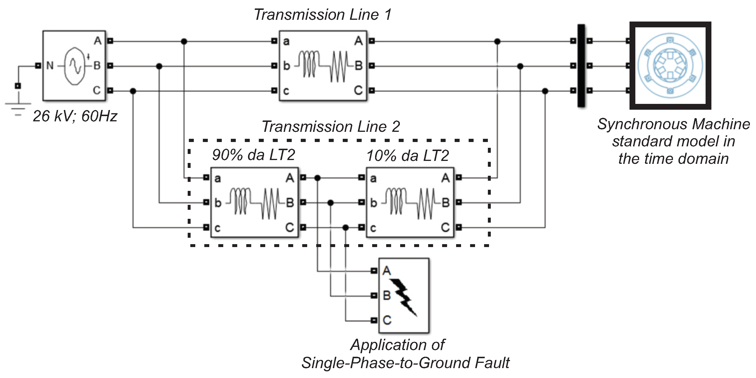
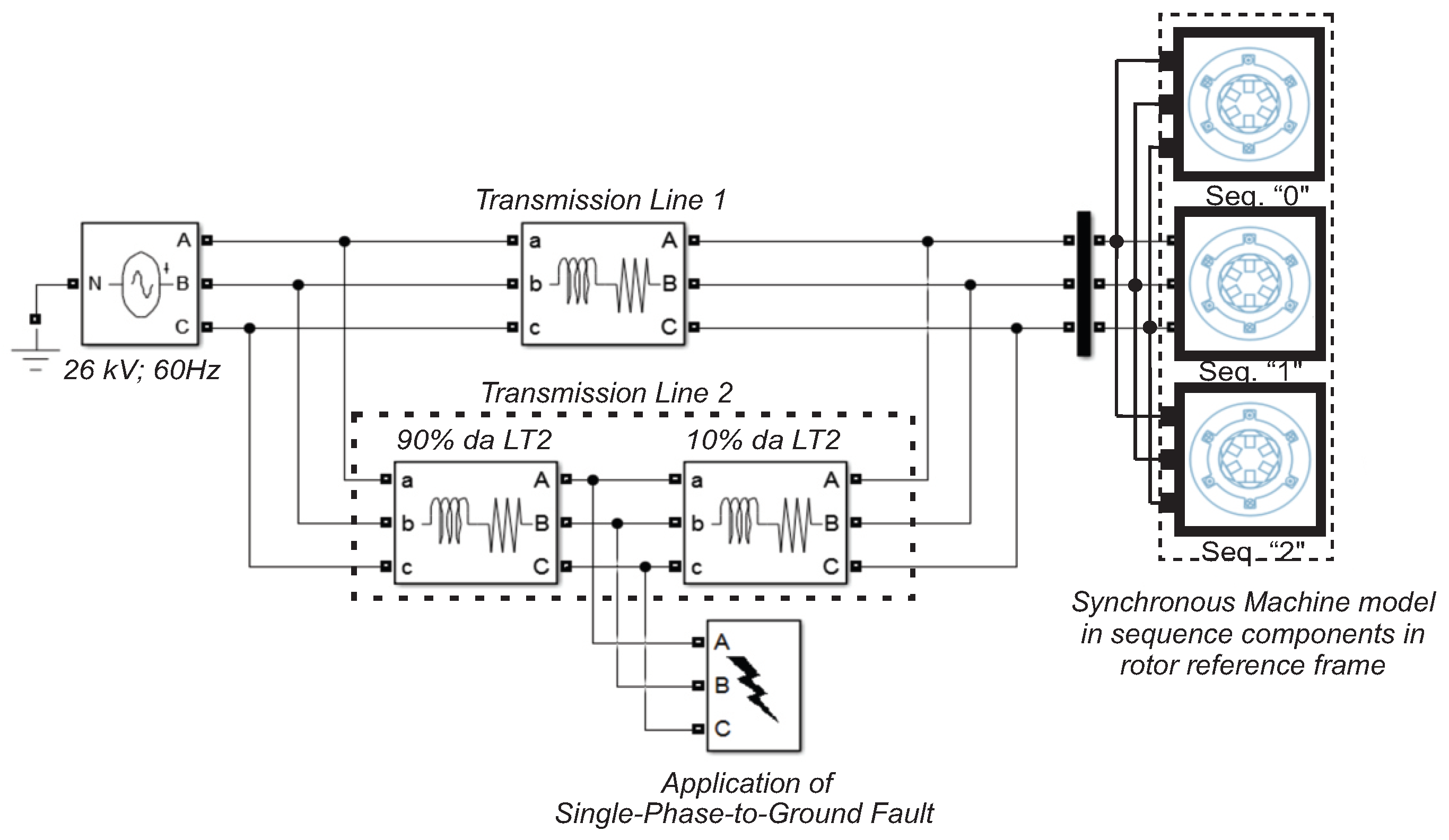
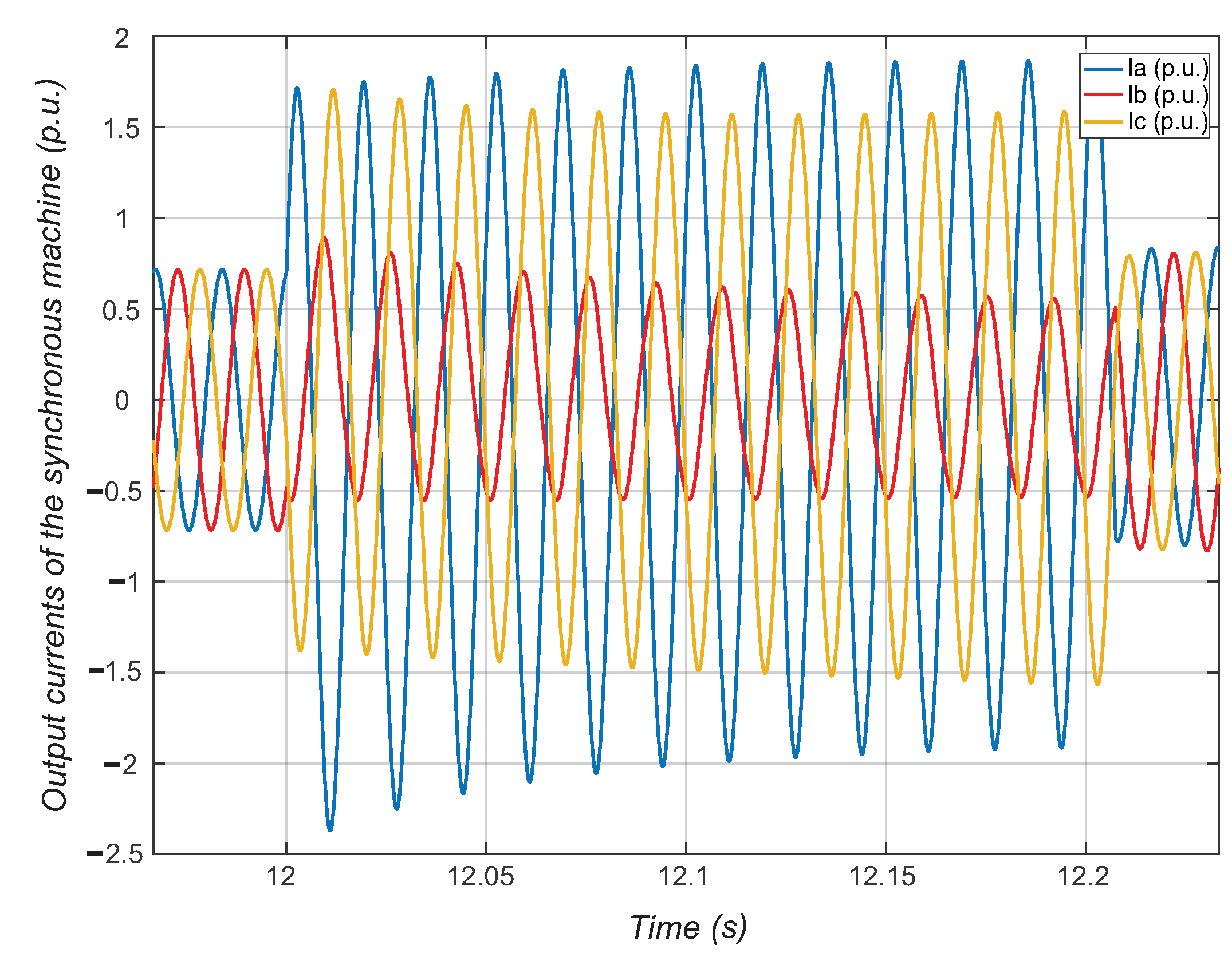
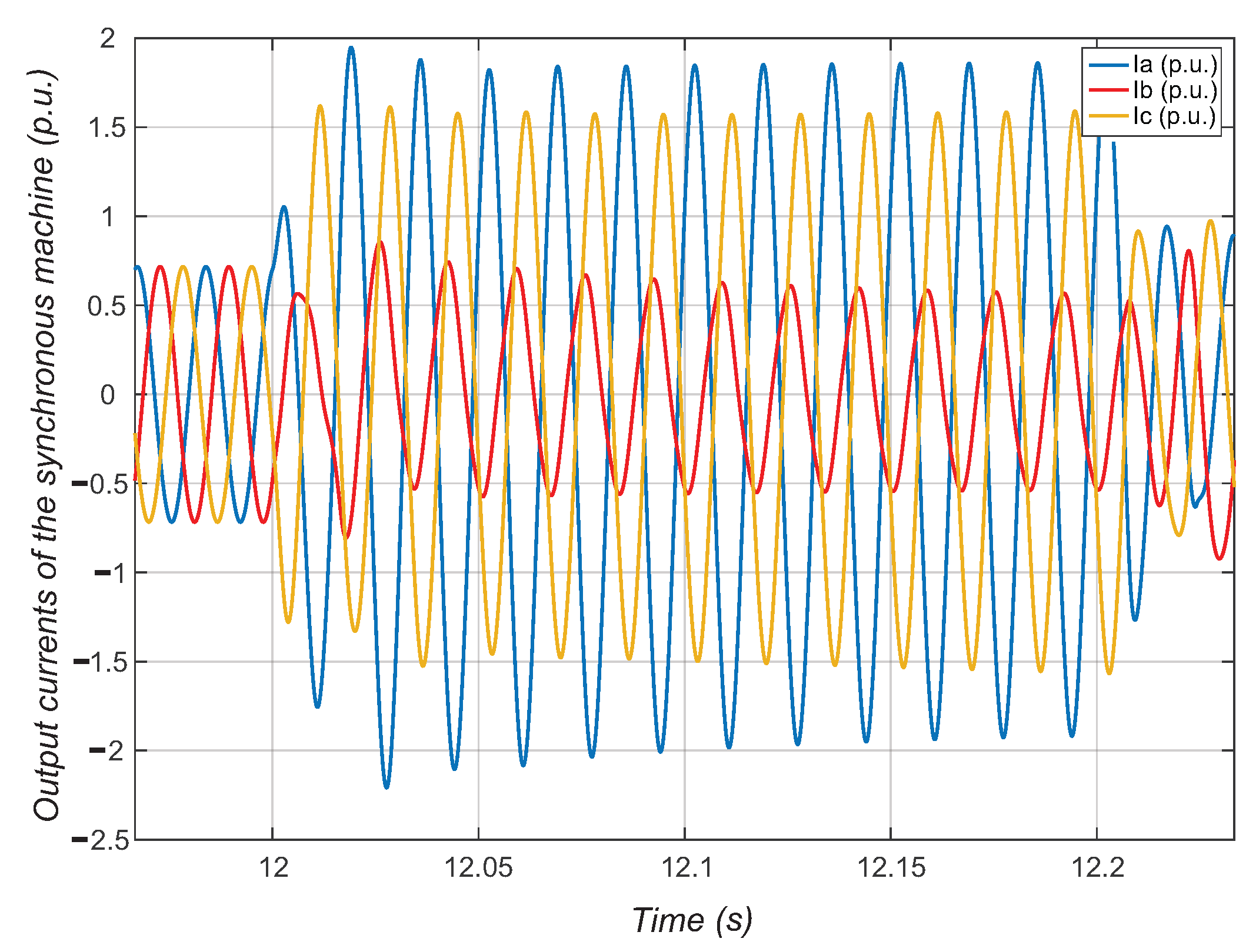
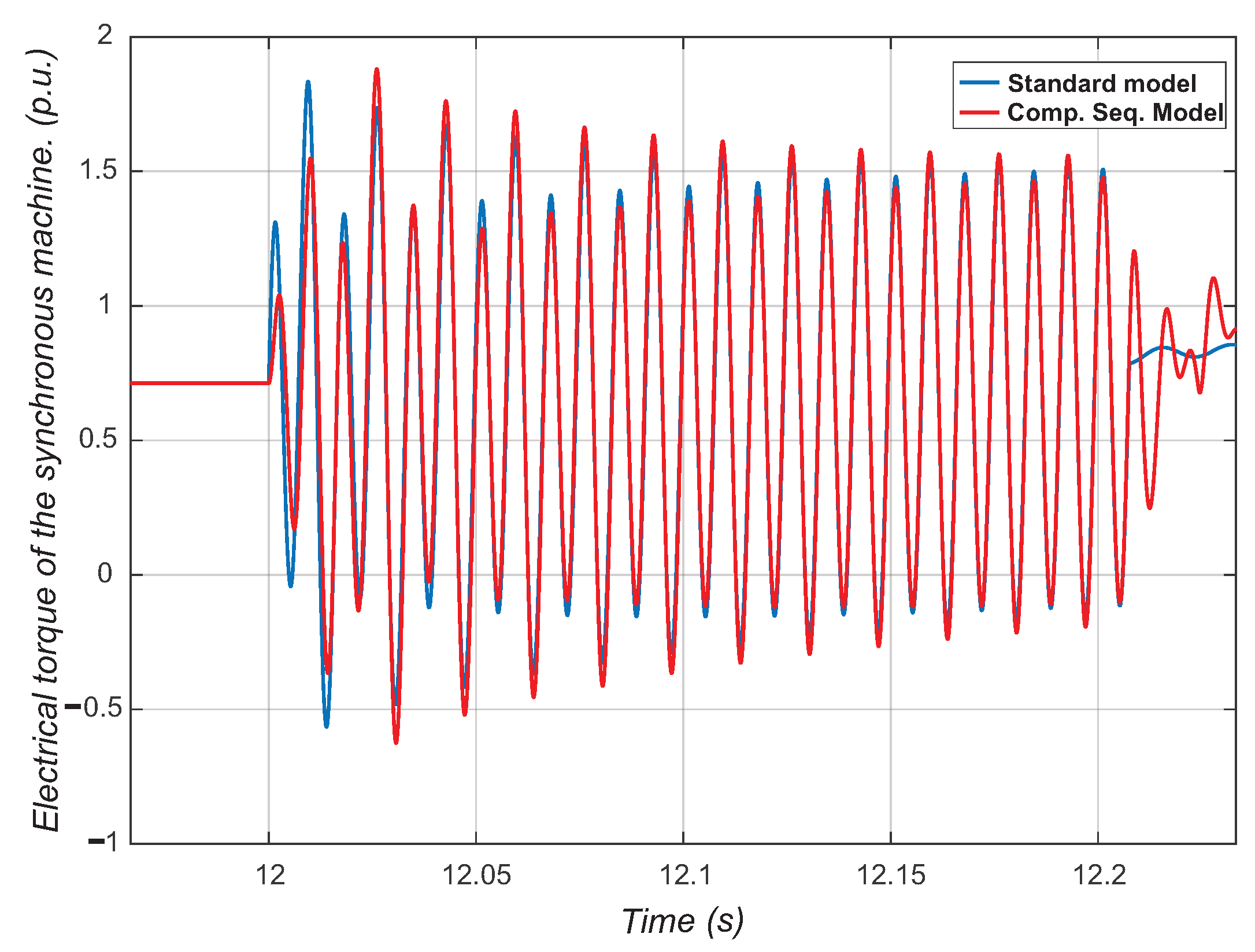
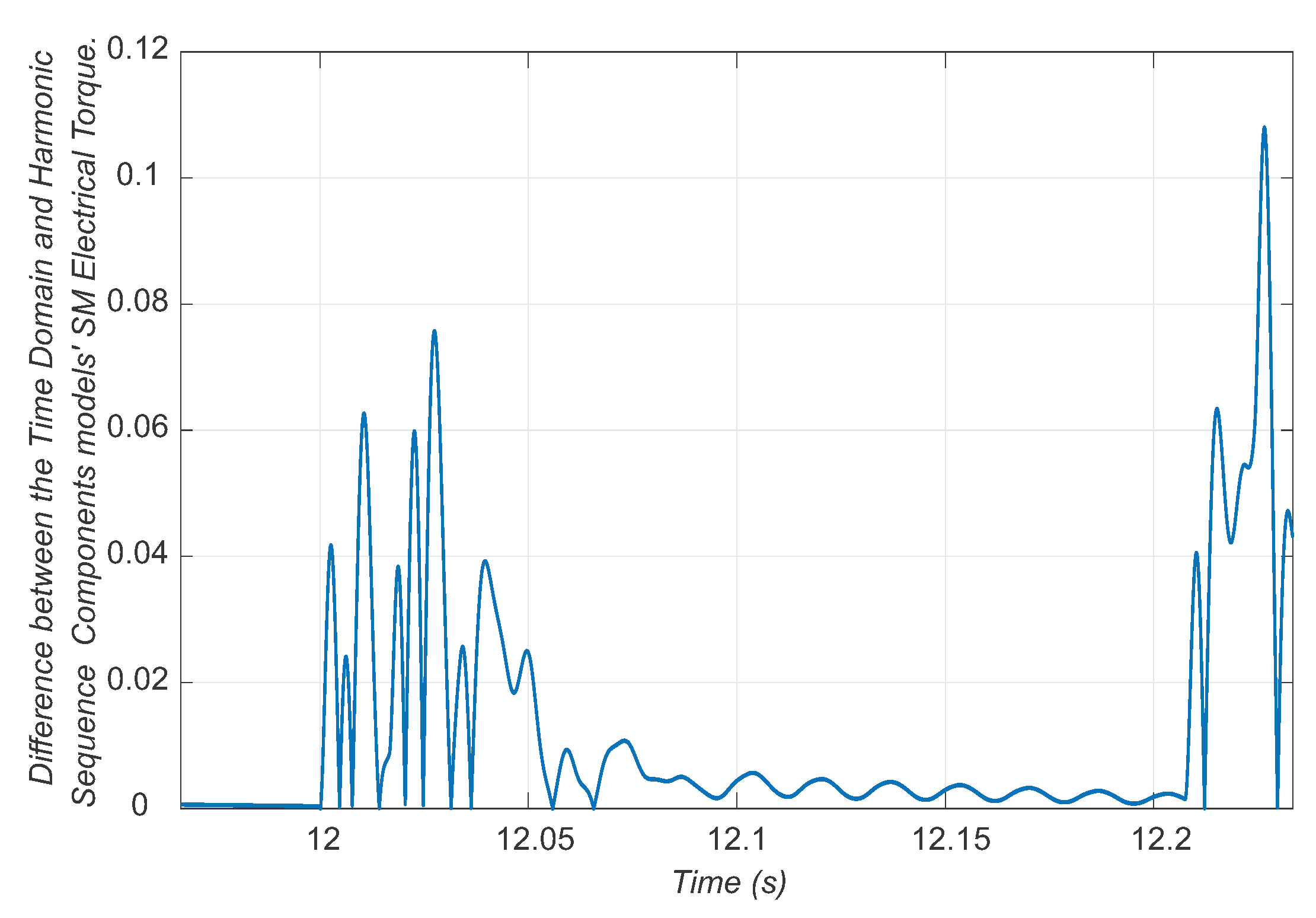
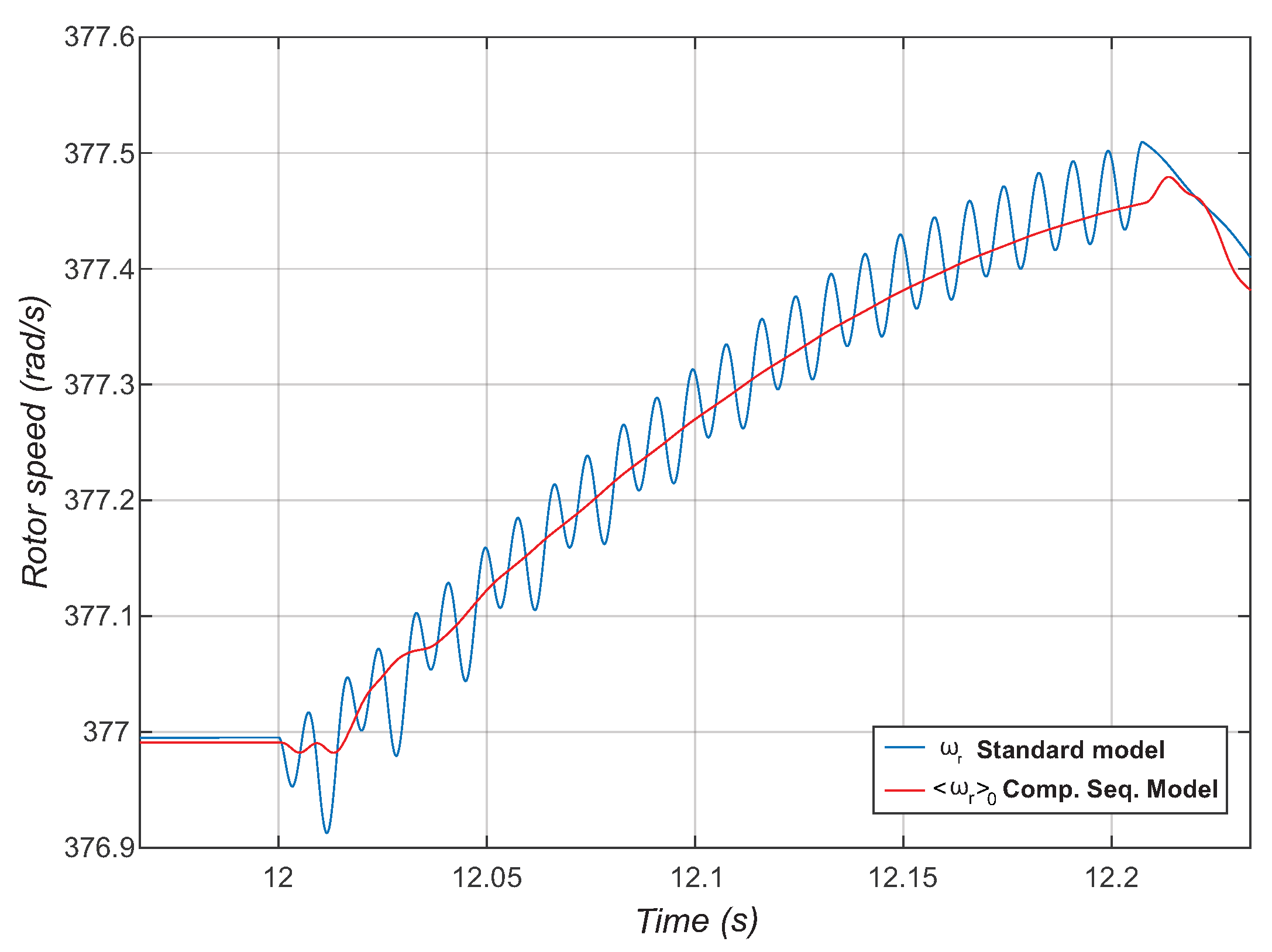
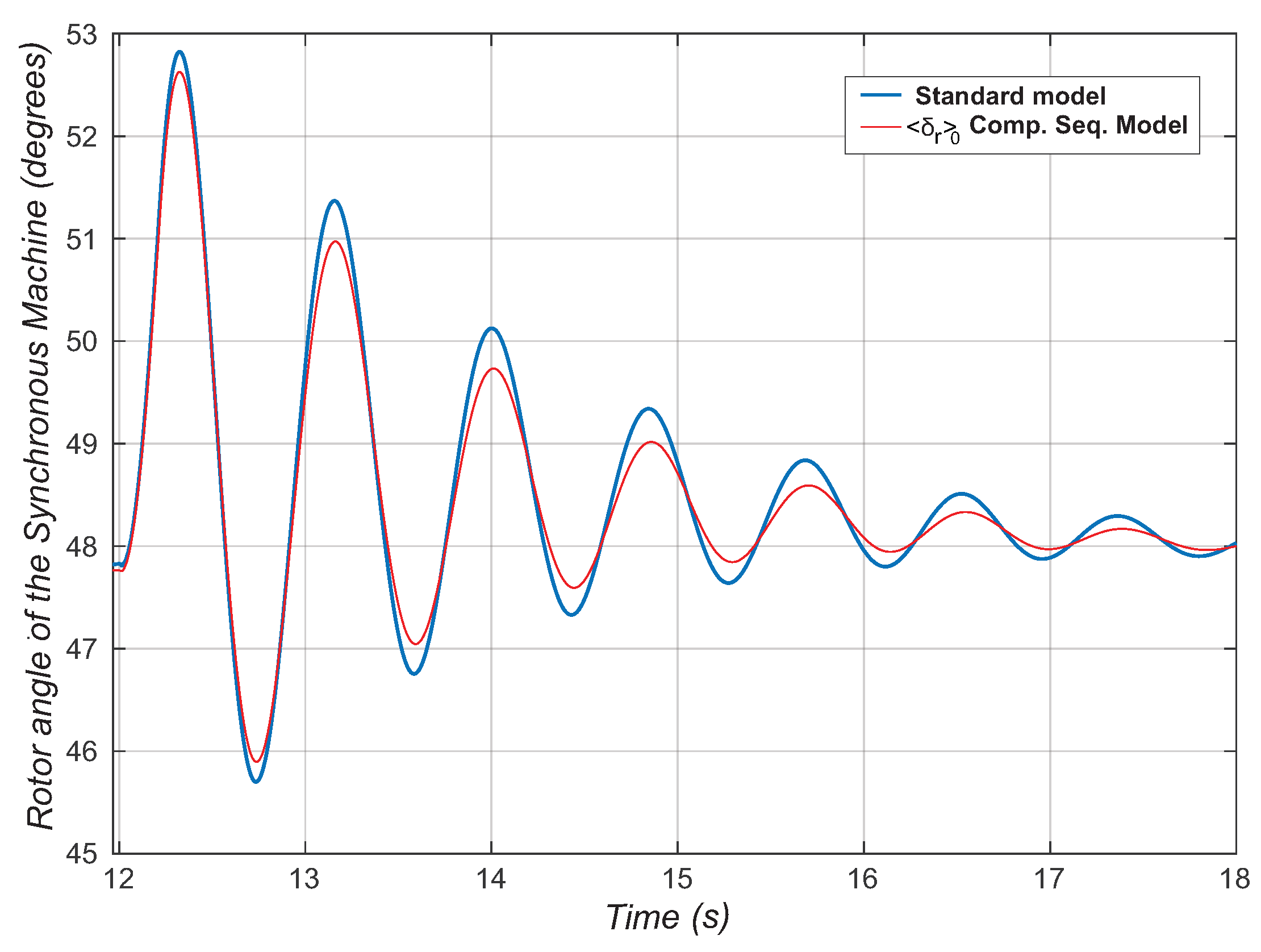
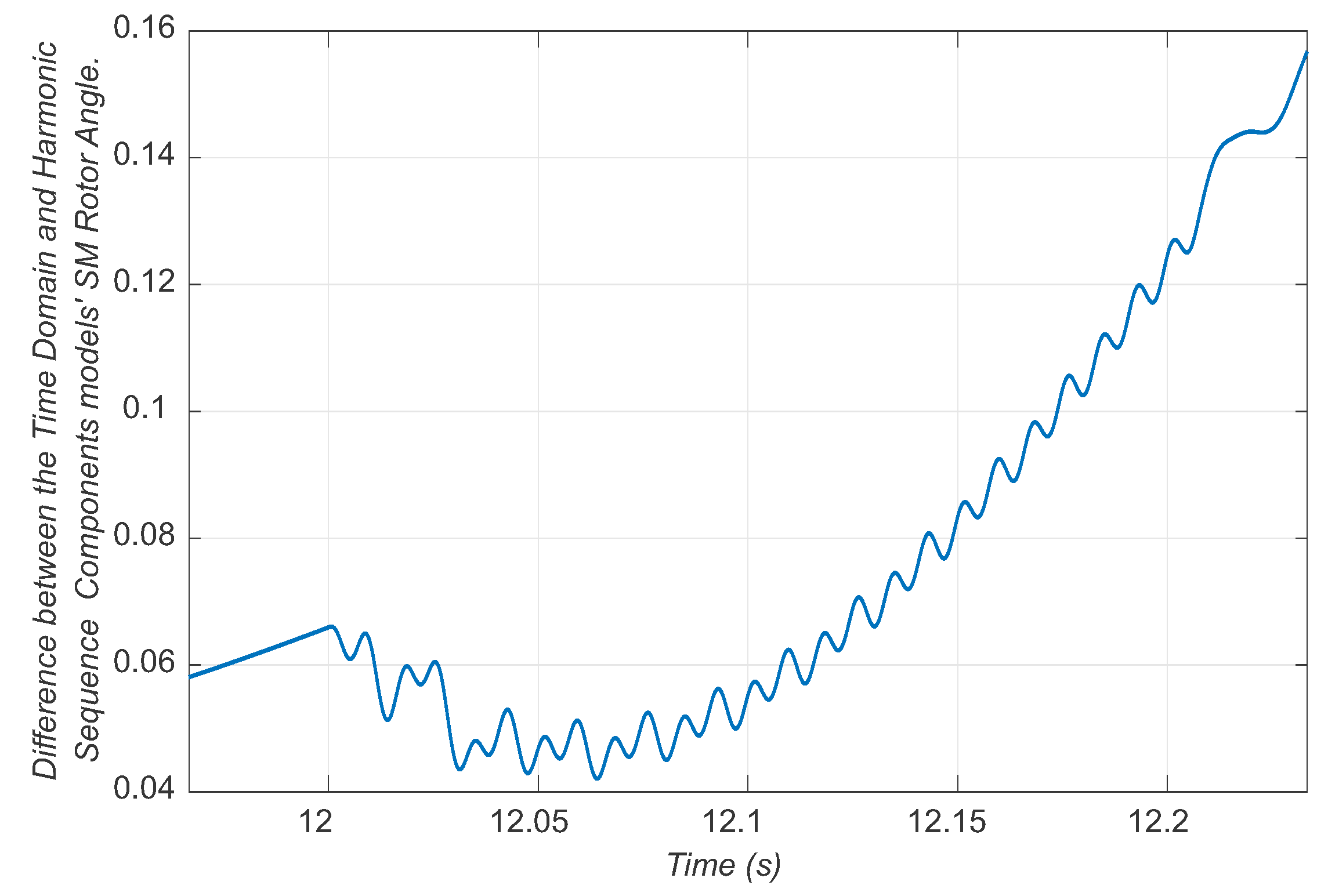
6. Comparison between Synchronous Machine Models in the Time Domain and Sequence Components

In this section, we present a comparison of simulations between the standard time-domain model and the model developed in Section 2.2 for synchronous machine components in harmonic sequence. The test system (Figure 1) consisted of a synchronous machine connected to an infinite bus via two transmission lines. A single-phase-to-ground fault was simulated, lasting 200 ms, occurring $90\%$ along the length of transmission line 2 from the infinite bus. Figure 2 depicts the system using the synchronous machine model in harmonic sequence components, where each synchronous machine represents a harmonic in the rotor reference, as determined by the equations for each $k=0,1,2$ of the model developed in Section 2.2.

The synchronous machine data are presented in

Table 1. Machine synchronous data.

$\mathit{S}=835$ MVA	V = 26 kV
$poles=2$	$cos\varphi =$ 0.85
$J={0.0658}^6$ J·s2, H = 5.6 s	$\omega$ = 3600 rpm
$X_{ls}=0.1538\Omega$, 0.9 p.u.	$r_s=0.00243\Omega$, 0.003 p.u.
$X_q=1.457\Omega$, 1.8 p.u.	$X_d=1.457\Omega$, 1.8 p.u.
$r_{kq1}=0.00144\Omega$, 0.00178 p.u.	$r_{fd}=0.00075\Omega$, 0.000929 p.u.
$X_{lkq1}=0.6578\Omega$, 0.8125 p.u.	$X_{lfd}=0.1145\Omega$, 0.1414 p.u.
$r_{kq2}=0.00681\Omega$, 0.00841 p.u.	$r_{kd}=0.01080\Omega$, 0.01334 p.u.
$X_{lkq2}=0.07602\Omega$, 0.0939 p.u.	$X_{lkd}=0.06577\Omega$, 0.08125 p.u.

.

The two transmission lines of the test electrical system had impedance values $R_{LT}$ = 0.0352 $\Omega$ or 0.0434 p.u. e $L_{LT}=0.0014H$ or 0.6414 p.u.

In Equation (26), the dependence of ${〈{\overline{T}}_e〉}_0$ on the harmonic currents considered in the rotor reference $k=0,1,2$ was demonstrated. However, in the simulation, a simplification was made by truncating the degree of the considered harmonics to $k=0$, thus obtaining the following definition:

$$\begin{array}{c}{〈{\overline{T}}_e〉}_0={\displaystyle \frac{X_{md}}{2}}\left({〈i_{fd}^r〉}_0+{〈i_{kd}^r〉}_0\right)\left({〈{\overrightarrow{i}}_{qds}^r〉}_0+{〈{\overrightarrow{i}}_{qds}^r〉}_0^{†}\right)\\ -j{\displaystyle \frac{X_{mq}}{2}}\left({〈i_{kq1}^r〉}_0+{〈i_{kq2}^r〉}_0\right)\left({〈{\overrightarrow{i}}_{qds}^r〉}_0-{〈{\overrightarrow{i}}_{qds}^r〉}_0^{†}\right)-j{\displaystyle \frac{X_{md}-X_{mq}}{4}}\left[{\left({〈{\overrightarrow{i}}_{qds}^r〉}_0\right)}^2-{\left({〈{\overrightarrow{i}}_{qds}^r〉}_0^{†}\right)}^2\right]\end{array}$$

(61)

This consideration is valid from the perspective of wanting to observe the impact of each degree of the harmonic considered in the equation of electrical torque, as can be seen in the following figures. The assumed simplification proved to be effective in providing a good approximation of the synchronous machine variables’ behavior through the sequence component model.

The simulation results for the standard time-domain model of the synchronous machine are shown in Figure 3 for the three-phase output currents of the synchronous machine, over approximately the 200 ms duration of the fault.

In Figure 4, the three-phase output currents of the synchronous machine using the harmonic sequence component model are shown.

From the comparison of Figure 3 and Figure 4, it can be observed that the behavior of the synchronous machine’s output currents is identical during pre-fault steady-state operation. During the disturbance, the behaviors are very close, except for the first two cycles of the transient when the fault is applied and when the fault is cleared. This difference is shown in Figure 5, where the maximum difference between the two models is 0.25 p.u. However, this difference does not significantly affect the rotor angle excursion, as is observed in the following.

In Figure 6, the electrical torque curves between the standard model and the sequence component model during the disturbance are compared. Similar to the currents, the torque exhibits very close behavior, except for the first two cycles of the transient. This difference, although considerable (since the results are per unit), does not significantly impact the rotor angle oscillations. It is worth clarifying that the electrical torque curve in the harmonic sequence component model was constructed from three values: ${〈{\overline{T}}_e〉}_0$, ${〈{\overline{T}}_e〉}_1$, and ${〈{\overline{T}}_e〉}_2$. The equations corresponding to the harmonic degree torques $k=1,2$ are not shown, but were considered in the simulations (to obtain these equations, substitute the value of $k=1,2$ in Equation (22)).

Similar to the analysis of the SM output currents, the difference between the electrical torque curves of the standard model and the harmonic sequence model is shown in Figure 7. The maximum difference between the two models is 0.08 p.u. during the transient when the fault is applied and 0.15 p.u. when the fault is cleared.

In Figure 8, a comparison between the curves of the average value of the electrical torque using the standard model and the curve of the electrical torque component $k=0$, i.e., ${〈{\overline{T}}_e〉}_0$ using the harmonic sequence component model is shown. The relevance of showing ${〈{\overline{T}}_e〉}_0$ lies in the fact that both variables, angular speed ${〈{\overline{\omega }}_r〉}_0$ and rotor angle ${〈{\delta }_r〉}_0$, are calculated as functions of ${〈{\overline{T}}_e〉}_0$. From the comparison, differences are observed between the curves shortly after the start and end of the disturbance. However, approximately from t = 12.05 s until the end of the fault at t = 12.2 s, the two curves are very close. Despite the differences at the beginning and end of the electrical torque curves, the rotor angle curve is not significantly different using the sequence component model, as can be observed.

In Figure 9, the synchronous machine rotor angular velocity curve ${\omega }_r$ for both synchronous machine models is shown. As mentioned in Figure 8, the term ${〈{\overline{\omega }}_r〉}_0$ is calculated solely from ${〈{\overline{T}}_e〉}_0$. A good agreement between the two curves is observed. However, the sequence components model fails to accurately reproduce the small oscillations during the transient period of the disturbance, as observed in the standard model. This is due to considering only the harmonic component $k=0$ in the electrical torque.

Figure 10 shows the difference between the rotor angular velocity curves of the standard model and the harmonic sequence model. As observed, the difference between both curves is the oscillatory component at double the fundamental frequency, which is expected and also observed in the electrical torque curve.

In Figure 11, the curve of the synchronous machine rotor angle $\left({\delta }_r\right)$ for both synchronous machine models is presented. A good agreement can be observed between the two curves during the disturbance and in the subsequent oscillations until reaching a point close to equilibrium. The difference in values between the two curves is less than $0.5$, allowing us to conclude that the sequence component model is suitable for approximating the rotor angle behavior. This conclusion is significant because the rotor angle is the variable used to assess the transient stability of the electrical system. Therefore, the harmonic sequence component model can be applied in the study of eigenvalue sensitivity.

The difference between the rotor angles of the standard model and the harmonic sequence model is shown in Figure 12. During the disturbance, the difference between the two curves is below ${0.5}^{\circ }$, which can be considered a good approximation depending on the focus of analysis, such as the transient stability of the SM. The curves for both models are in phase and oscillate around the same new equilibrium rotor angle after the fault is cleared.

7. Sensitivity Analysis of the Test System

The sensitivity analysis was applied to the test system using the equations presented in Section 4 and Section 5. The results of the sensitivity analysis with respect to the angular velocity ${\omega }_r$ and angle ${\delta }_r$ of the synchronous machine rotor are shown in

Table 2. Eigenvalues’ sensitivity analysis of the test system.

${\mathit{\lambda }}_{\mathit{i}}$	Real Part of ${\mathit{\lambda }}_{\mathit{i}}$	Freq. (Hz)	Sensitivity $\left({\mathit{\omega }}_{\mathit{r}}\right)$	Sensitivity $\left({\mathit{\delta }}_{\mathit{r}}\right)$	Dominant Variable
1–2	−5.5	$\pm 60$	−0.3	0.6	-
3	−65.1	0	−3.7	−3.3	$c,a,d$
4	−27.2	0	−1.6	2.0	$f,b,e$
5	0	0	0	0	-
6–7	−3	$\pm 1.9$	2.9	−0.1	$b,e$
8	−0.3	0	−0.001	0.5	-
9–10	−5.4	$\pm 120$	−0.2	0	-
11–12	−5.4	$\pm 0.1$	−0.2	0	-
13–14	−69.5	$\pm 60$	0.3	0	-
15–16	−28.6	$\pm 60$	0.02	0	-
17–18	−0.7	$\pm 60$	0	0	-
19–20	0	$\pm 60$	0	0	-
21–22	−5.44	$\pm 180$	−0.2	0	-
23–24	−5.44	$\pm 60$	−0.2	0	-
25–26	−69.5	$\pm 120$	0.3	0	-
27–28	−28.6	$\pm 120$	0.02	0	-
29–30	−0.7	$\pm 120$	0	0	-
31–32	0	$\pm 120$	0	0	-

Note: The highest sensitivities are in red.

.

From the results shown in Table 2, the highest sensitivity values can be observed in red. The sensitivity results with respect to ${\omega }_r$ and ${\delta }_r$ indicate the same oscillation modes (3 and 4) as critical modes, except for the even-mode (6–7) indicated solely by the sensitivity with respect to ${\omega }_r$.

Once the critical modes are identified, one can determine through the study of participation factors those state variables that had the greatest impact on these critical oscillation modes and therefore would be the variables with the highest impact on the variation of ${\omega }_r$ and ${\delta }_r$. These high-impact variables are shown in the last column of Table 2, where each letter represents a state variable defined as:

• a represents ${〈{\overrightarrow{i}}_{qds}^r〉}_0^R$ in dynamic phasors,
• b represents ${〈{\overrightarrow{i}}_{qds}^r〉}_0^I$ in dynamic phasors,
• c represents ${〈i_{kq1}^r〉}_0^R$ in dynamic phasors,
• d represents ${〈i_{kq2}^r〉}_0^R$ in dynamic phasors,
• e represents ${〈i_{fd}^r〉}_0^R$ in dynamic phasors,
• f represents ${〈i_{kd}^r〉}_0^R$ in dynamic phasors.

Among the dynamic phasor current variables in the rotor reference frame with the highest impact, the variable that can be manipulated during disturbances by injecting current provided by the inverter is the stator current of the synchronous machine, specifically the current ${〈{\overrightarrow{i}}_{qds}^r〉}_0$ (real and imaginary parts). As seen in (41), this current in the rotor reference frame is a consequence of the current in the $FFSP$ component in the stationary reference frame. Therefore, it is concluded that the inverter should inject current in the $FFSP$ component following the proposed control strategy, to reduce the oscillations of the synchronous machine rotor angle during control action.

8. Conclusions

This paper presented a synchronous machine modeled using the harmonic sequence component model with dynamic phasors in the rotor reference frame. This model accurately represented the dynamic behavior of the synchronous machine when subjected to a single-phase fault, as evidenced by comparisons with time-domain simulations. The stability analysis was conducted over the first two to three cycles of the disturbance. Although the harmonic sequence component model yielded a smaller oscillation amplitude of the synchronous machine’s rotor angle, the observed difference from the time-domain model was less than ${0.5}^{\circ }$ during the fault, indicating an accurate representation. This provides confidence in using the model for small-signal stability analysis to identify critical modes through a sensitivity analysis of the eigenvalues concerning the rotor angular velocity and angle. Both variables were chosen due to their characteristic dynamic response under an asymmetric fault.

After identifying the critical modes, a participation factor analysis revealed that the DC component of the stator current represented as ${〈{\overrightarrow{i}}_{qds}^r〉}_0$ significantly participated in eigenvalues with critical damping. This was related to the fundamental frequency component of the synchronous machine’s stator current in the stationary reference frame. From this conclusion, a control strategy can be proposed to improve the critical modes and mitigate potential instabilities caused by asymmetric faults in a synchronous machine.

The main contributions of this paper are as follows:

• We developed the state equation of a synchronous machine using the harmonic sequence component model;
• We used the state equation to perform a sensitivity analysis of the eigenvalues. The objective was to evaluate the effect of asymmetrical faults on the synchronous machine by determining critical modes through a sensitivity analysis of the rotor angular velocity and rotor angle;
• A participation factor analysis identified harmonic components with significant participation in the critical modes;
• While this paper focused on analyzing the impact of asymmetric faults on the dynamic behavior of a synchronous machine, the developed mathematical model can be applied to various operating conditions, provided that a sensitivity analysis is conducted on the variables directly affected by the contingency under consideration.

The proposed mathematical model is a useful tool for identifying harmonic sequence components that significantly impact critical modes affected by specific contingencies, enabling the implementation of appropriate control strategies to mitigate negative effects and enhance system damping to avoid potential instabilities.

For future research, the harmonic sequence component model should be validated in multi-machine power systems to assess its accuracy in representing all components of the electrical system. If discrepancies increase, the model may need to be expanded to include broader harmonic content, although this would increase the complexity of the analysis and computational effort required.

References

1. Krause, P.C.; Wasynczuk, O.; Sudhoff, S.D.; Pekarek, S. Analysis of Electric Machinery and Drive Systems; Wiley Online Library: Hoboken, NJ, USA, 2002; Volume 2. [Google Scholar]
2. Caliskan, V.A.; Verghese, O.; Stankovic, A.M. Multifrequency averaging of DC/DC converters. IEEE Trans. Power Electron. 1999, 14, 124–133. [Google Scholar] [CrossRef]
3. Sanders, S.R. On limit cycles and the describing function method in periodically switched circuits. IEEE Trans. Circuits Syst. I Fundam. Theory Appl. 1993, 40, 564–572. [Google Scholar] [CrossRef]
4. Stankovic, A.M.; Sanders, S.R.; Aydin, T. Dynamic phasors in modeling and analysis of unbalanced polyphase AC machines. IEEE Trans. Energy Convers. 2002, 17, 107–113. [Google Scholar] [CrossRef]
5. De Rua, P.; Sakinci, Ö.C.; Beerten, J. Comparative study of dynamic phasor and harmonic state-space modeling for small-signal stability analysis. Electr. Power Syst. Res. 2020, 189, 106626. [Google Scholar] [CrossRef]
6. Sakinci, Ö.C.; Beerten, J. Generalized dynamic phasor modeling of the MMC for small-signal stability analysis. IEEE Trans. Power Deliv. 2019, 34, 991–1000. [Google Scholar] [CrossRef]
7. Wang, X.; Blaabjerg, F. Harmonic stability in power electronic-based power systems: Concept, modeling, and analysis. IEEE Trans. Smart Grid 2018, 10, 2858–2870. [Google Scholar] [CrossRef]
8. Lyu, J.; Zhang, X.; Cai, X.; Molinas, M. Harmonic state-space based small-signal impedance modeling of a modular multilevel converter with consideration of internal harmonic dynamics. IEEE Trans. Power Electron. 2018, 34, 2134–2148. [Google Scholar] [CrossRef]
9. Yue, X.; Wang, X.; Blaabjerg, F. Review of small-signal modeling methods including frequency-coupling dynamics of power converters. IEEE Trans. Power Electron. 2018, 34, 3313–3328. [Google Scholar] [CrossRef]
10. Yang, T.; Bozhko, S.; Asher, G. Assessment of dynamic phasors modelling technique for accelerated electric power system simulations. In Proceedings of the 2011 14th European Conference on Power Electronics and Applications, Birmingham, UK, 30 August–1 September 2011; pp. 1–9. [Google Scholar]
11. Chudasama, M.C.; Kulkarni, A.M. Dynamic phasor analysis of SSR mitigation schemes based on passive phase imbalance. IEEE Trans. Power Syst. 2010, 26, 1668–1676. [Google Scholar] [CrossRef]
12. Demiray, T.; Andersson, G.; Busarello, L. Evaluation study for the simulation of power system transients using dynamic phasor models. In Proceedings of the 2008 IEEE/PES Transmission and Distribution Conference and Exposition: Latin America, Bogota, Colombia, 13–15 August 2008; pp. 1–6. [Google Scholar]
13. Bai, X.; Jiang, T.; Guo, Z.; Yan, Z.; Ni, Y. A unified approach for processing unbalanced conditions in transient stability calculations. IEEE Trans. Power Syst. 2006, 21, 85–90. [Google Scholar] [CrossRef]
14. Kotian, S.M.; Shubhanga, K. Dynamic phasor modelling and simulation. In Proceedings of the 2015 Annual IEEE India Conference (INDICON), New Delhi, India, 17–20 December 2015; pp. 1–6. [Google Scholar]
15. Meersman, B.; Degroote, L.; Renders, B.; Vandevelde, L. Simulating transients in electrical power systems using dynamic phasors. In Proceedings of the Proc. IEEE Benelux Young Researchers Symposium in Electrical Power Engineering (YRS’08), Eindhoven, The Netherlands, 7–8 February 2008. [Google Scholar]
16. Stankovic, A.M.; Aydin, T. Analysis of asymmetrical faults in power systems using dynamic phasors. IEEE Trans. Power Syst. 2000, 15, 1062–1068. [Google Scholar] [CrossRef]
17. Huang, S.; Song, R.; Zhou, X. Analysis of balanced and unbalanced faults in power systems using dynamic phasors. In Proceedings of the International Conference on Power System Technology, Kunming, China, 13–17 October 2002; Volume 3, pp. 1550–1557. [Google Scholar]
18. Novotny, D.W.; Lipo, T.A. Vector Control and Dynamics of AC Drives; Oxford University Press: Oxford, UK, 1996; Volume 41. [Google Scholar]
19. Kundur, P.S.; Balu, N.J.; Lauby, M.G. Power system dynamics and stability. Power Syst. Stab. Control 2017, 3, 700–701. [Google Scholar]
20. Nolan, P.J.; Sinha, N.K.; Alden, R.T. Eigenvalue sensitivities of power systems including network and shaft dynamics. IEEE Trans. Power Appar. Syst. 1976, 95, 1318–1324. [Google Scholar] [CrossRef]
Figure 1. Test system with a synchronous machine in the sequence component model.
Energies 17 03634 g001
Figure 2. Test system with a synchronous machine in the standard model and sequence component model.
Energies 17 03634 g002
Figure 3. Output currents of the synchronous machine using the standard time-domain model.
Energies 17 03634 g003
Figure 4. Output currents of the synchronous machine using the harmonic sequence component model.
Energies 17 03634 g004
Figure 5. Difference between the FFSP component in the time-domain and harmonic sequence models of the SM output currents in p.u.
Energies 17 03634 g005
Figure 6. Comparison of electrical torque between the standard model and the harmonic sequence component model.
Energies 17 03634 g006
Figure 7. Difference between the electrical torque in the time-domain and harmonic sequence models of the SM in p.u.
Energies 17 03634 g007
Figure 8. Comparison of average electrical torque from the standard model and T ¯ e 0 from the harmonic sequence component model.
Energies 17 03634 g008
Figure 9. Comparison of ω r between the standard model and the value ω ¯ r 0 of the harmonic sequence component model during transient.
Energies 17 03634 g009
Figure 10. Difference between the angular velocity in the time-domain and harmonic sequence models of the SM in (rad/s).
Energies 17 03634 g010
Figure 11. Comparison of rotor angle δ r between the standard model and the harmonic sequence component model.
Energies 17 03634 g011
Figure 12. Difference between the rotor angle in the time-domain and harmonic sequence models of the SM in (degrees).
Energies 17 03634 g012