
Local Energy Community to Support Hydrogen Production and Network Flexibility


Abstract
:1. Introduction
2. Problem Formulation
- Type I loads: They consume a fixed amount of total energy during the scheduling period and can switch between on and off states. While turned on, their output is a fixed value. Also, the required total energy must be provided within a given operating time window. Examples are water pumps, washing machines, and electric vehicles.
- Type II loads: They also need to consume a fixed amount of total energy, can be switched on and off during a given operating time window, and operate with a fixed power value. However, they also cannot be turned off consecutively for more than a few hours. Examples are refrigerators and freezers.
- Type III loads: Differently from the previous two, they only have a lower boundary for the energy to be provided within the assigned operating time window. They can be switched on and off and can adjust their power consumption continuously. However, their power supply must be above a certain threshold for them to be turned on.
2.1. Objective Function
2.2. Grid Constraints
2.3. DG Constraints
2.4. BESSs Constraints
2.5. Controllable Load Constraints
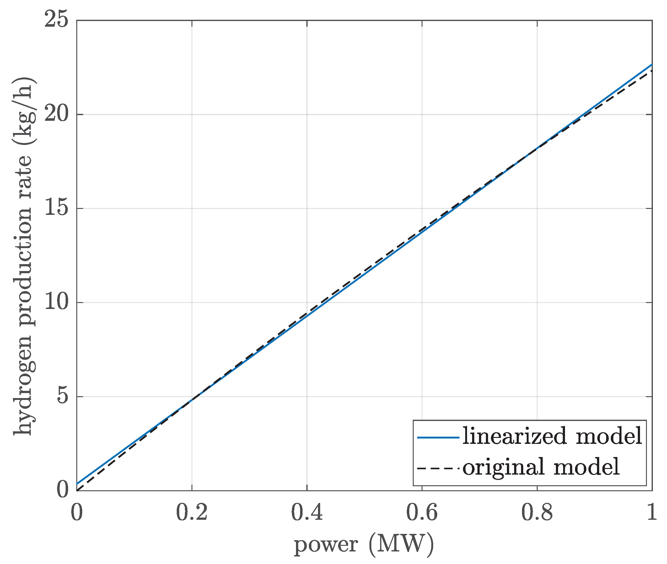
2.6. Electrolyzer Constraints
2.7. Solution Method
3. Numerical Application
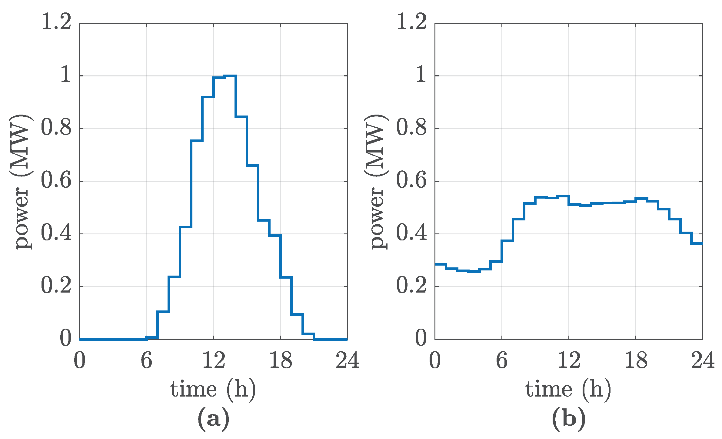
3.1. Case Studies
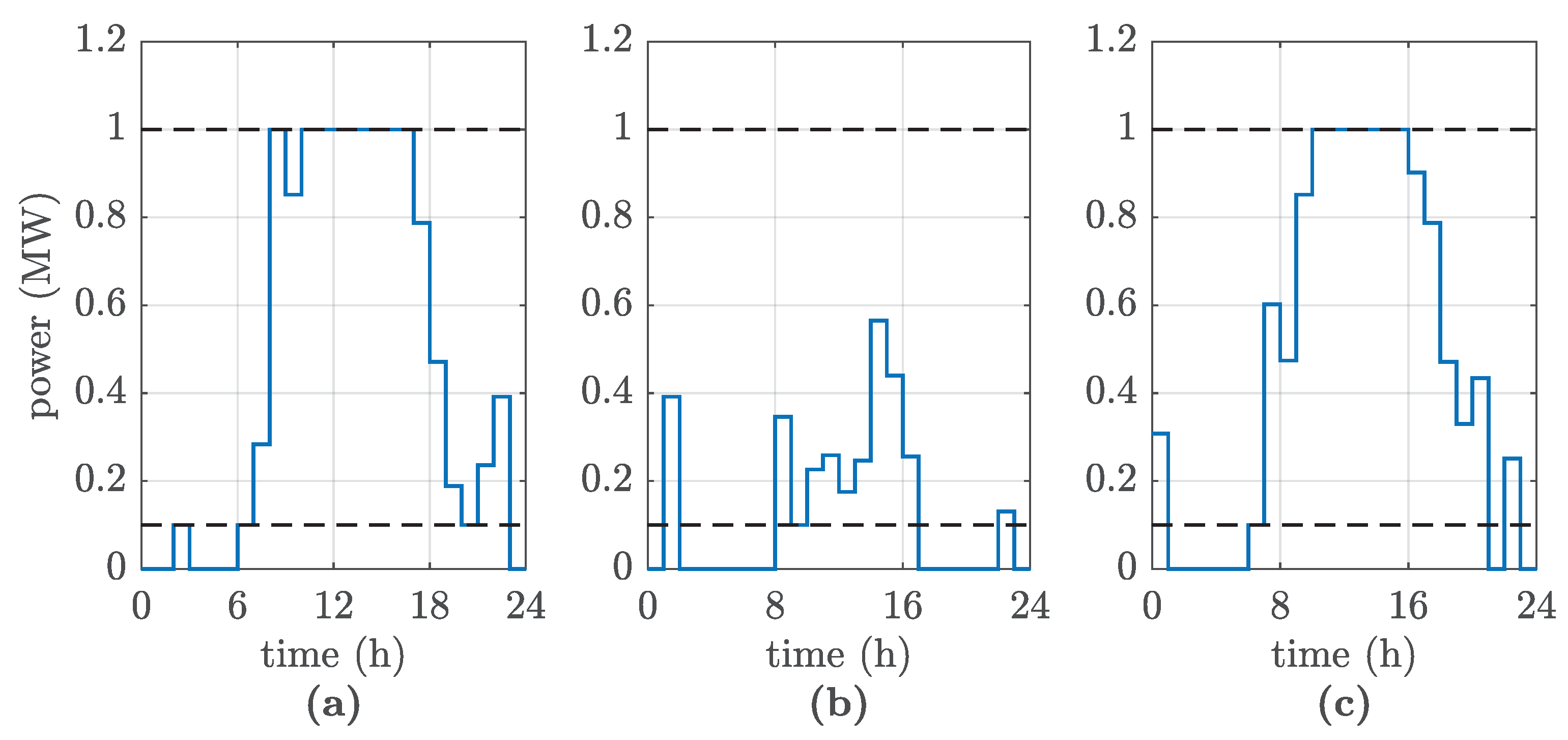
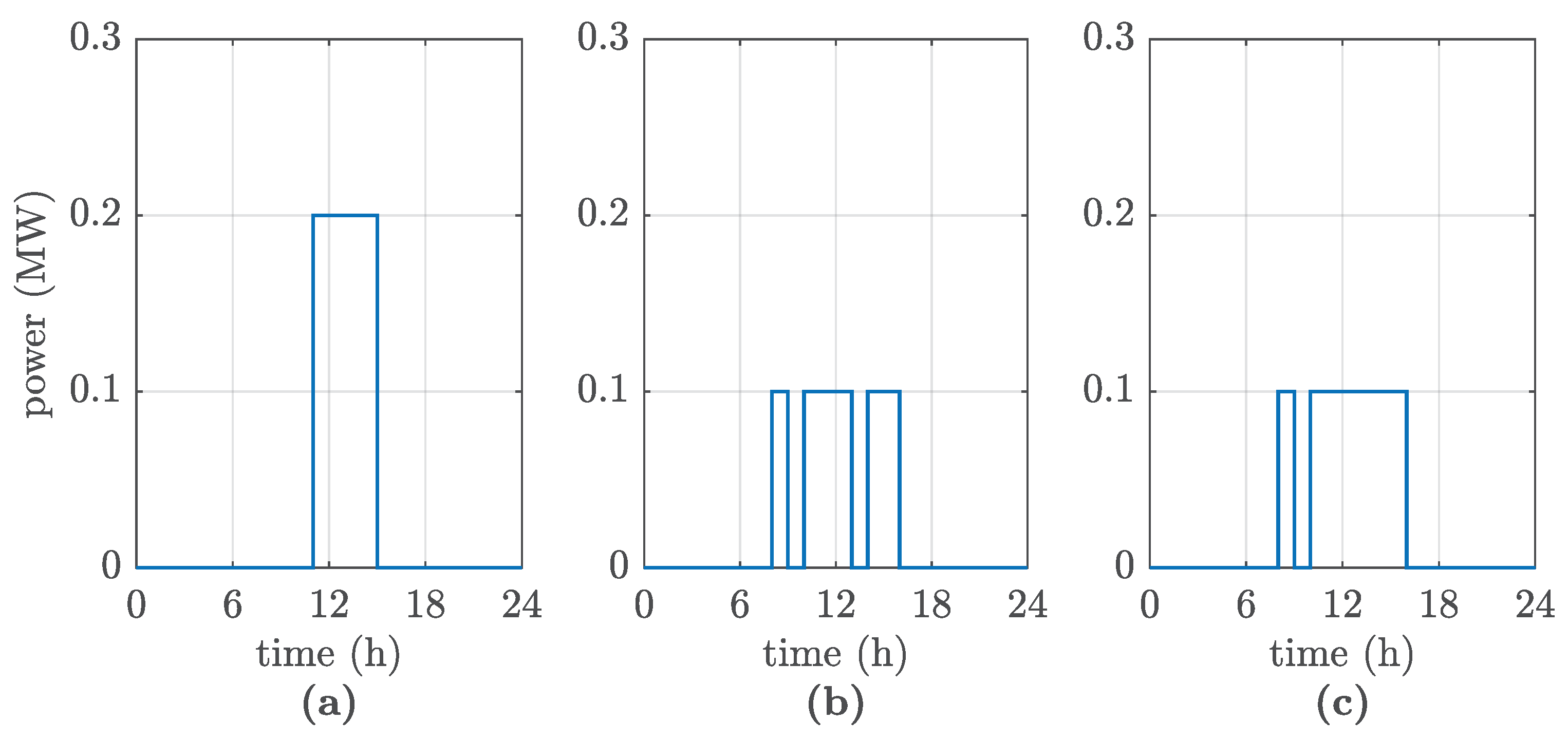
3.2. Results
4. Conclusions
Author Contributions
Funding
Data Availability Statement
Conflicts of Interest
List of Symbols
| Constants and Parameters | |
| Daily energy target required by the i-th type I controllable load | |
| Daily energy target required by the i-th type II controllable load | |
| Minimum daily energy required by the i-th type III controllable load | |
| Number of time steps during which the i-th type II controllable must be turned on for every operating period lasting time intervals | |
| Beginning of | |
| End of | |
| Power absorbed by the i-th type I controllable load when turned on | |
| Power absorbed by the i-th type II controllable load when turned on | |
| Time step | |
| Faraday’s efficiency | |
| Charging efficiency of the i-th BESS | |
| Discharging efficiency of the i-th BESS | |
| Scheduling window of the i-th type I controllable load | |
| Scheduling window of the i-th type II controllable load | |
| Scheduling window of the i-th type III controllable load | |
| Susceptance of the nodal admittance matrix relative to buses i and j | |
| Temperature coefficient of the equivalent internal resistance of an electrolyzer cell | |
| Reversible electrolyzer cell potential in standard conditions | |
| Reversible voltage of an electrolyzer cell | |
| F | Faraday’s constant |
| Conductance of the nodal admittance matrix relative to buses i and j | |
| k | Discrete time index |
| Molar mass of molecular hydrogen | |
| Daily time intervals | |
| Number of BESSs | |
| Number of cells in the electrolyzer stack | |
| Number of DG units | |
| Number of REC members | |
| p | Electrolyzer pressure |
| Standard pressure | |
| Maximum active charging power which can be provided by the i-th BESS | |
| Maximum active discharging power which can be provided by the i-th BESS | |
| Rated power of the electrolyzer | |
| Maximum power that the i-th type III controllable load can absorb | |
| Minimum power that the i-th type III controllable load can absorb when turned on | |
| Hydrogen sell price | |
| Reactive energy price | |
| Incentive price for shared energy | |
| Maximum reactive power which can be provided by the i-th BESS | |
| Minimum reactive power which can be provided by the i-th BESS | |
| Maximum reactive power which can be provided by the i-th DG unit | |
| Minimum reactive power which can be provided by the i-th DG unit | |
| Number of time steps defining the windows during which the i-th type II controllable load must work for at least time intervals | |
| R | Universal gas constant |
| Equivalent internal resistance of a single electrolyzer cell in standard conditions | |
| Equivalent internal resistance of a single electrolyzer cell | |
| Maximum allowed SoC for the ith battery | |
| Minimum allowed SoC for the ith battery | |
| T | Electrolyzer temperature |
| Standard temperature | |
| Maximum allowed voltage | |
| Minimum allowed voltage | |
| Variables | |
| Phase angle between voltages at buses i and j | |
| Rate of hydrogen production during time step k | |
| Shared energy during time step k | |
| Objective function | |
| Current in a single electrolyzer cell | |
| Hydrogen produced during time step k | |
| Active charging power of the i-th BESS during time step k | |
| Overall active charging power of the REC members’ BESSs during time step k | |
| Active discharging power of the i-th BESS during time step k | |
| Overall active discharging power of the REC members’ BESSs during time step k | |
| Active power generated by the i-th DG unit during time step k | |
| Overall active power generated by the REC members’ DG units during time step k | |
| Active power absorbed by the electrolyzer during time step k | |
| Active power absorbed by the electrolyzer in continuous time | |
| Active power injected at bus i of the network during time step k | |
| Active power absorbed by the i-th type III load when turned on | |
| Non-controllable load of the i-th REC member during time step k | |
| Type III controllable load of the i-th REC member during time step k | |
| Type II controllable load of the i-th REC member during time step k | |
| Type I controllable load of the i-th REC member during time step k | |
| Overall active power absorbed by the REC members’ loads during time step k | |
| Reactive power provided by the i-th BESS during time step k | |
| Rective power provided by the i-th DG unit during time step k | |
| Reactive power injected at bus i of the network during time step k | |
| Reactive power provided by the REC resources during time step k | |
| SoC of the i-th battery at time step k | |
| t | Continuous time |
| Voltage of a single electrolyzer cell | |
| Voltage magnitude at bus i during time step k | |
References
- Taibi, E.; Miranda, R.; Vanhoudt, W.; Winkel, T.; Lanoix, J.C.; Barth, F. Hydrogen from Renewable Power: Technology Outlook for the Energy Transition; International Renewable Energy Agency: Masdar City, United Arab Emirates, 2018. [Google Scholar]
- Flexibility Resources Task Force. Increasing Electric Power System Flexibility: The Role of Industrial Electrification and Green Hydrogen Production. Technical Report. 2022. Available online: https://www.esig.energy/increasing-electric-power-system-flexibility/ (accessed on 24 June 2024).
- Energy Systems Integration Group. Assessing the Flexibility of Green Hydrogen in Power System Models. Technical Report. 2024. Available online: https://www.esig.energy/green-hydrogen-in-power-system-models/ (accessed on 24 June 2024).
- Daneshvar, M.; Mohammadi-Ivatloo, B.; Zare, K.; Asadi, S. Transactive energy management for optimal scheduling of interconnected microgrids with hydrogen energy storage. Int. J. Hydrogen Energy 2021, 46, 16267–16278. [Google Scholar] [CrossRef]
- Shahbazbegian, V.; Shafie-khah, M.; Laaksonen, H.; Strbac, G.; Ameli, H. Resilience-oriented operation of microgrids in the presence of power-to-hydrogen systems. Appl. Energy 2023, 348, 121429. [Google Scholar] [CrossRef]
- Tostado-Véliz, M.; Arévalo, P.; Jurado, F. A comprehensive electrical-gas-hydrogen Microgrid model for energy management applications. Energy Convers. Manag. 2021, 228, 113726. [Google Scholar] [CrossRef]
- Tomin, N.; Kurbatsky, V.; Suslov, K.; Gerasimov, D.; Serdyukova, E.; Yang, D. Flexibility-based improved energy hub model for multi-energy distribution systems. In Proceedings of the CIRED Porto Workshop 2022: E-Mobility and Power Distribution Systems, Porto, Portugal, 2–3 June 2022; Volume 2022, pp. 409–413. [Google Scholar] [CrossRef]
- Ban, M.; Yu, J.; Shahidehpour, M.; Yao, Y. Integration of power-to-hydrogen in day-ahead security-constrained unit commitment with high wind penetration. J. Mod. Power Syst. Clean Energy 2017, 5, 337–349. [Google Scholar] [CrossRef]
- Wu, T.; Wang, J.; Yue, M. On the Integration of Hydrogen Into Integrated Energy Systems: Modeling, Optimal Operation, and Reliability Assessment. IEEE Open Access J. Power Energy 2022, 9, 451–464. [Google Scholar] [CrossRef]
- Zhao, P.; Gu, C.; Cao, Z.; Hu, Z.; Zhang, X.; Chen, X.; Hernando-Gil, I.; Ding, Y. Economic-Effective Multi-Energy Management Considering Voltage Regulation Networked with Energy Hubs. IEEE Trans. Power Syst. 2021, 36, 2503–2515. [Google Scholar] [CrossRef]
- Ponnaganti, P.; Sinha, R.; Pillai, J.R.; Bak-Jensen, B. Flexibility provisions through local energy communities: A review. Next Energy 2023, 1, 100022. [Google Scholar] [CrossRef]
- Javadi, M.S.; Osório, G.J.; Cardoso, R.J.A.; Catalão, J.P.S. Towards Reducing Electricity Costs in an Energy Community Equipped with Home Energy Management Systems and a Local Energy Controller. In Proceedings of the 2023 IEEE Conference on Control Technology and Applications (CCTA), Bridgetown, Barbados, 16–18 August 2023; pp. 746–751. [Google Scholar] [CrossRef]
- Chiş, A.; Rajasekharan, J.; Lundén, J.; Koivunen, V. Demand response for renewable energy integration and load balancing in smart grid communities. In Proceedings of the 2016 24th European Signal Processing Conference (EUSIPCO), Budapest, Hungary, 29 August–2 September 2016; pp. 1423–1427. [Google Scholar] [CrossRef]
- Marrasso, E.; Martone, C.; Pallotta, G.; Roselli, C.; Sasso, M. Assessment of energy systems configurations in mixed-use Positive Energy Districts through novel indicators for energy and environmental analysis. Appl. Energy 2024, 368, 123374. [Google Scholar] [CrossRef]
- He, Y.; Zhou, Y.; Yuan, J.; Liu, Z.; Wang, Z.; Zhang, G. Transformation towards a carbon-neutral residential community with hydrogen economy and advanced energy management strategies. Energy Convers. Manag. 2021, 249, 114834. [Google Scholar] [CrossRef]
- Rabiee, A.; Keane, A.; Soroudi, A. Green hydrogen: A new flexibility source for security constrained scheduling of power systems with renewable energies. Int. J. Hydrogen Energy 2021, 46, 19270–19284. [Google Scholar] [CrossRef]
- Pastore, L.M.; Lo Basso, G.; Quarta, M.N.; de Santoli, L. Power-to-gas as an option for improving energy self-consumption in renewable energy communities. Int. J. Hydrogen Energy 2022, 47, 29604–29621. [Google Scholar] [CrossRef]
- Spazzafumo, G.; Raimondi, G. Economic assessment of hydrogen production in a Renewable Energy Community in Italy. E-Prime-Adv. Electr. Eng. Electron. Energy 2023, 4, 100131. [Google Scholar] [CrossRef]
- Shen, J.; Jiang, C.; Li, B. Controllable Load Management Approaches in Smart Grids. Energies 2015, 8, 11187–11202. [Google Scholar] [CrossRef]
- Stekli, J.; Bai, L.; Cali, U. Pricing for Reactive Power and Ancillary Services in Distribution Electricity Markets. In Proceedings of the 2021 IEEE Power & Energy Society Innovative Smart Grid Technologies Conference (ISGT), Washington, DC, USA, 16–18 February 2021; pp. 1–5. [Google Scholar] [CrossRef]
- Ng, S.K.K.; Zhong, J. Security-constrained dispatch with controllable loads for integrating stochastic wind energy. In Proceedings of the 2012 3rd IEEE PES Innovative Smart Grid Technologies Europe (ISGT Europe), Berlin, Germany, 14–17 October 2012. [Google Scholar]
- Yue, M.; Lambert, H.; Pahon, E.; Roche, R.; Jemei, S.; Hissel, D. Hydrogen energy systems: A critical review of technologies, applications, trends and challenges. Renew. Sustain. Energy Rev. 2021, 146, 111180. [Google Scholar] [CrossRef]
- Buttler, A.; Spliethoff, H. Current status of water electrolysis for energy storage, grid balancing and sector coupling via power-to-gas and power-to-liquids: A review. Renew. Sustain. Energy Rev. 2018, 82, 2440–2454. [Google Scholar] [CrossRef]
- Sarrias-Mena, R.; Fernández-Ramírez, L.M.; García-Vázquez, C.A.; Jurado, F. Electrolyzer models for hydrogen production from wind energy systems. Int. J. Hydrogen Energy 2015, 40, 2927–2938. [Google Scholar] [CrossRef]
- Allahham, A.; Greenwood, D.; Patsios, C.; Walker, S.L.; Taylor, P. Primary frequency response from hydrogen-based bidirectional vector coupling storage: Modelling and demonstration using power-hardware-in-the-loop simulation. Front. Energy Res. 2023, 11, 1217070. [Google Scholar] [CrossRef]
- Atlam, O.; Kolhe, M. Equivalent electrical model for a proton exchange membrane (PEM) electrolyser. Energy Convers. Manag. 2011, 52, 2952–2957. [Google Scholar] [CrossRef]
- Italian Ministry of the Environment and Energy Security, MASE (in Italian). Decree n. 414, 07/12/2023. 2023. Available online: https://www.mase.gov.it/sites/default/files/Decreto%20CER.pdf (accessed on 24 June 2024).
- Mottola, F.; Proto, D.; Russo, A. Probabilistic planning of a battery energy storage system in a hybrid microgrid based on the Taguchi arrays. Int. J. Electr. Power Energy Syst. 2024, 157, 109886. [Google Scholar] [CrossRef]
- Carmo, M.; Fritz, D.L.; Mergel, J.; Stolten, D. A comprehensive review on PEM water electrolysis. Int. J. Hydrogen Energy 2013, 38, 4901–4934. [Google Scholar] [CrossRef]
- Majumdar, A.; Haas, M.; Elliot, I.; Nazari, S. Control and control-oriented modeling of PEM water electrolyzers: A review. Int. J. Hydrogen Energy 2023, 48, 30621–30641. [Google Scholar] [CrossRef]
- Pan, G.; Gu, W.; Lu, Y.; Qiu, H.; Lu, S.; Yao, S. Optimal Planning for Electricity-Hydrogen Integrated Energy System Considering Power to Hydrogen and Heat and Seasonal Storage. IEEE Trans. Sustain. Energy 2020, 11, 2662–2676. [Google Scholar] [CrossRef]
- Pan, G.; Gu, W.; Wu, Z.; Lu, Y.; Lu, S. Optimal design and operation of multi-energy system with load aggregator considering nodal energy prices. Appl. Energy 2019, 239, 280–295. [Google Scholar] [CrossRef]
- Strunz, K.; Abbasi, E.; Fletcher, R.; Hatziargyriou, N.; Iravani, R.; Joos, G. TF C6.04.02: TB 575—Benchmark Systems for Network Integration of Renewable and Distributed Energy Resources. 2014. Available online: https://www.e-cigre.org/publications/detail/575-benchmark-systems-for-network-integration-of-renewable-and-distributed-energy-resources.html (accessed on 24 June 2024).
- IRENA. Green Hydrogen Cost Reduction: Scaling Up Electrolysers to Meet the 1.5 °C Climate Goal; International Renewable Energy Agency: Masdar City, United Arab Emirates, 2020. [Google Scholar]
- Database from the GECAD PV System. IEEE Open Data Sets. Available online: https://site.ieee.org/pes-iss/data-sets (accessed on 24 June 2024).
- Dufo-López, R.; Lujano-Rojas, J.M.; Bernal-Agustín, J.L.; Artal-Sevil, J.S.; Bayod-Rújula, Á.A.; Cortés-Arcos, T.; Oñate, J.C.; Martínez, C.E. Utility-scale renewable hydrogen generation by wind turbines. Renew. Energy Power Qual. J. 2023, 21, 19–24. [Google Scholar] [CrossRef]


| N.C. Load | PV 1 | PV 2 | Electrolyzer | BESS 1 | BESS 2 | |
|---|---|---|---|---|---|---|
| Bus | #4, #5, #9, #12, #14, #15 | #12 | #14 | #7 | #4 | #9 |
| Rating | 100 kW | 1 MW | 1 MW | 1 MW | 0.5 MW 2 MWh | 0.5 MW 2 MWh |
| Type I | Type II | Type III | |
|---|---|---|---|
| (kW) | 200 | 100 | - |
| (kWh) | 800 | 600 | 400 |
| 08:00–16:00 | 06:00–18:00 | 08:00–16:00 | |
| - | - | 10 | |
| - | - | 100 | |
| - | 2 | - | |
| - | 4 | - |
| Case 1 | Case 2 | Case 3 | |
|---|---|---|---|
| Produced H2 [kg] | 262.9 | 74.0 | 262.9 |
| Shared energy [MWh] | 14.123 | 6.767 | 14.123 |
| Revenue [EUR] | 2015 | 847 | 2035 |
Disclaimer/Publisher’s Note: The statements, opinions and data contained in all publications are solely those of the individual author(s) and contributor(s) and not of MDPI and/or the editor(s). MDPI and/or the editor(s) disclaim responsibility for any injury to people or property resulting from any ideas, methods, instructions or products referred to in the content. |
© 2024 by the authors. Licensee MDPI, Basel, Switzerland. This article is an open access article distributed under the terms and conditions of the Creative Commons Attribution (CC BY) license (https://creativecommons.org/licenses/by/4.0/).
Share and Cite
Ferrara, M.; Mottola, F.; Proto, D.; Ricca, A.; Valenti, M. Local Energy Community to Support Hydrogen Production and Network Flexibility. Energies 2024, 17, 3663. https://doi.org/10.3390/en17153663
Ferrara M, Mottola F, Proto D, Ricca A, Valenti M. Local Energy Community to Support Hydrogen Production and Network Flexibility. Energies. 2024; 17(15):3663. https://doi.org/10.3390/en17153663
Chicago/Turabian StyleFerrara, Massimiliano, Fabio Mottola, Daniela Proto, Antonio Ricca, and Maria Valenti. 2024. "Local Energy Community to Support Hydrogen Production and Network Flexibility" Energies 17, no. 15: 3663. https://doi.org/10.3390/en17153663