Abstract
The heat treatment temperature must precisely meet the required profile to ensure the quality of the workpiece. The model of the heat treatment furnace is not precisely known because it is nonlinear and complex. Considering this aspect, model-free temperature control methods are proposed, which are not based on a model of the process, but only on the input and output data acquired from the control system. Since the controlled temperature must accurately track the reference formed by the ramp and soak signals in the presence of disturbances, model-free iPI controllers were chosen due to the included double-integral component that ensures the steady-state performance for ramp signals. For the tuning of the iPI controller parameters, the iterative feedback tuning method is proposed, and the performance is compared with that obtained using the sliding mode control iPI variant. The proposed iPI control laws are tested for ramp and soak scenarios, using temperature suitable to thermal treatment technological processes, and performance is analyzed using both process-specific indices and classical criteria.
1. Introduction
The control of technological processes represents an important component in the field of control engineering. Worldwide, industrial activity is reaching unprecedented levels and production systems are becoming more and more complex. Against the background of this development, control theory must present solutions through which the production process can achieve the highest possible efficiency. Along with the improvement of the technological installations, the role of the measuring devices involved in the process were taken over by numerous sensors, based on which the processes can be monitored more easily, and they provide information in real time, an aspect that also helps in following the measurements over a longer period of time. This advantage offered by systems that have a multitude of sensors can be brilliantly used in the field of control engineering, with numerous data-driven control (DDC) strategies being developed. These are methods by which the systems no longer require modeling, which most of the time is not the most accurate, but realizes, based on the data collected from the process, various approximations and modeling valid for a short period of time, online. A comparison of the DDC and model-based control (MBC) methods is presented by Hou in [1,2]. Practically, through this approach, the disadvantage of having a complex system, which is difficult to model, is transformed into an advantage, with the laws from the DDC category having a high accessibility.
Model-free control (MFC), introduced by Fliess and Join in [3], is one of the methods from the DDC class. Such a method uses intelligent PID (iPID) controllers, which have applicability in various fields such as being used for motion control of a forestry crane [4], finger dynamics in a myoelectric-based prosthetic hand [5], lateral vehicle control [6], and machine tool application [7]. Another advantage of this control method is that the way the control laws are formulated offers an integral component by default, which ensures a zero-position error. Moreover, an iPI- or iPID-type law will therefore have two integral components, which will make such laws suitable for applications where the existence of a control law with two integral components is necessary, as in the case of direct torque control of PMSM [8] and glycemia regulation of type-1 diabetes [9].
Iterative feedback tuning (IFT) is another strategy in the DDC category, defined by Hjalmarsson in [10], that is being used by many methods to improve tuning results, such as in PID controllers [11], robust controllers [12], and PIDs tuned with fuzzy logic controllers [13]. As [14] shows, MFC and IFT can be used together, within an iterative algorithm, to improve the control results with the iPID controllers introduced by [3]. Through this new approach, the algorithm starts from a stable response of the system obtained with iPID control law, and after the iterative procedure, new parameters of the controller are obtained, which lead to an improvement of the response by minimizing a criterion using signals acquired from the control system.
Sliding mode control (SMC) is a control method used for nonlinear plants, offering good robustness in situations of parameter variations and disturbances. It is used in various applications such as wind turbine control [15], hydrogen–renewable energy power systems [16], and control of nuclear reactor cores for electricity generation [17]. The advantages of SMC include improvements over an MFC law, as [18] shows. Therefore, control laws of the type iPD-SMC and iPI-SMC were defined in [19]. Such laws were used to control a PMSM speed-control system [20,21], nonlinear nonaffine dynamic systems [22], and nonlinear underactuated systems with uncertainties and disturbances [23].
Heat treatment systems are some of the technological processes that have evolved a lot over time, with some of the current versions being complex ones containing a multitude of sensors. Such systems thus become amenable to being controlled by DDC methods, as in [24]. Thermal treatment systems are useful in various applications such as the treatment of various alloys or products such as 65Mn low-alloy steel [25], carbon membranes [26], tempering of medium carbon steels [27], or carbon fiber–reinforced plastics (CFRP) processing [28]. In addition to the DDC approach for the control of such systems, an AI approach for quality improvement in heat treatment processing is analyzed in [29], a PID control is presented in [30], a fuzzy PID is used in [31], while in [32], the research on heat treatment control technology of machining parts is presented. This aspect becomes more and more important in the context of modern materials that require certain thermal treatments applied with high precision, which offer very good structure, durability, and resistance. In [24], an iPI controller designed using the pole-placement method and using the IFT algorithm with an identity matrix for the iterative computation of tuning parameters was proposed.
The present work aims to expand the subject by analyzing some model-free control laws for applications in the field of heat treatment systems. In the following sections, control laws of the iPI-IFT and iPI-SMC type for heat treatment scenarios used in industry for various alloys will be comparatively analyzed. The control laws will be applied to highlight the advantage offered by a two-component integral controller concluded in [24]. A new algorithm is presented in [24] that allows obtaining specific performances for the control of heat treatment processes. The main problem with such tunings is the reference type for which the iPI tuning law solution was chosen because it has a built-in double integrator. Unfortunately, the double-integrator component provides good steady-state performance for ramp–soak-type references, but certain problems are noticed in the transient response. The typical performances of the transient regime were solved by the means of the following two solutions: iPI-IFT and iPI-SMC. The design methods of the two algorithms are presented in detail and a comparative analysis of the performances of the two iPI control variants will be carried out, using performance indices specific to heat treatment systems. The testing of the controllers and the performance analysis were carried out following the simulations, with the results highlighting the superior performance of the conjugate control laws, compared to the initial iPI variant.
This paper presents the following contributions, relative to the state of the art:
- -
- Temperature control of heat treatment processes with ramp–soak references, through an iPI controller with an integrated double integrator;
- -
- Design of an iPI controller using data-driven IFT technology, for temperature control, within the thermal treatment processes;
- -
- Choosing the initial parameters of the iPI law that ensure system stability for the initial iteration of the IFT algorithm, using the Jury test;
- -
- Use of a conjugate control law of the iPI-SMC type for temperature control in heat treatment processes;
- -
- Comparative analysis based on performance indices specific to temperature control in heat treatment processes for iPI-IFT- and iPI-SMC-type controllers.
The structure of the paper is as follows: Section 2 will detail the aspects regarding the heat treatment scenarios analyzed and the thermal system used, Section 3 will present the model-free control laws used, Section 4 will present the results obtained from the simulations, while the conclusions will be presented in Section 5.
2. Temperature Control
Thermal treatment systems have increased importance in industry, both in the case of metal alloys and semiconductors. For all these materials, a technological process is necessary to confer increased durability and robustness, to withstand the various types of environments in which they are used. Most of the time, in the case of metal treatment, it is necessary to obtain some microstructures through which the alloy is more resistant and does not degrade quickly over time. This treatment is cyclical, in which the material is heated to certain high temperatures, followed by a baking phase, in which the high temperature is maintained for a longer period, to finally achieve cooling.
The 65Mn alloy is one that offers a high flexibility, but also a suitable rigidity, being used for metal springs, but also for rotary blades, friction clutches, and brakes. Another advantage presented in [25] is related to the resistance to long-term stress and heavy-loading working conditions. The main disadvantage is the excessive wear that can occur under the previously specified conditions of use. Therefore, to prevent excessive wear, it is necessary to develop some microstructures that improve the mechanical properties of the alloy. One of the methods by which this effect can be obtained is a heat treatment, which requires high precision to obtain the desired effect.
Several experimental variants were considered in [25], both regarding the chemical composition and the way in which the thermal treatment is applied. A proposed solution consists of a two-phase treatment, the first being a solid treatment, which involves raising the temperature to 900 °C, followed by oil cooling. The second phase is what distinguishes this type of heat treatment from others, being composed of a sequence of four heating–cooling cycles. The heating part is carried out at 10 °C per second, from room temperature to 810 °C, after which the temperature is maintained for 5 min. After this temperature level, a cooling takes place at room temperature, and the process is repeated four times, as shown in Figure 1, named as “cyclic quenching times” in [25].
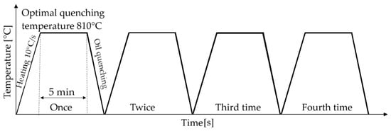
Figure 1.
Temperature profile for the quenching scenario.
Another application that requires a heat treatment with a precision tracking of the reference is that applied to carbon membranes. Such membranes will be used in the future for CO2 filtration applications to reduce energy consumption. They can be manufactured by thermal treatment of some polymers that are their precursors. The main elements that characterize such membranes are stability at certain pressures and temperatures, chemical resistance, gas separation, pervaporation, vapor permeation, and liquid filtration.
To create such membranes, there are a multitude of methods, which provide for the treatment of chemical compounds in various environments, with various temperature profiles, as in [26]. Moreover, there are various approaches, some with cyclic sequences, but others use a single sequence since the membrane is a sensitive one and can be damaged in the situation where several thermal treatments are applied. In addition to the carbon component used, other materials and polymers are used in the process, which help support the membrane and give it rigidity or elasticity, porosity and breathability, depending on the application for which the membrane is created. The process considered in [26] provides for a drying of the polymer membrane overnight at 60 °C, after which the actual treatment follows. This takes place in a nitrogen environment, under 200 mL/min. The treatment has two main phases as follows: a stabilization is carried out at 350 °C, for 30 min, followed by a carbonization at 700 °C for another 30 min, to finally cool the membrane to an ambient temperature. The graphical representation of the temperature variation during the entire process is depicted in Figure 2.
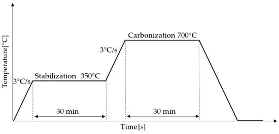
Figure 2.
Temperature profile for the stabilization–carbonization scenario.
To simulate the previously described thermal treatments, which require a precise tracking of the ramp–soak reference temperature, the model of a furnace will be used, as described in [27]. It includes two media as follows: the temperature of the first being controlled by a heater coil incorporated in the second medium with temperature , in the presence of the temperature of the external environment. The inner room is the one in which the thermal treatment must be carried out, the temperature being the output value of the system. A graphical representation of this can be seen in Figure 3.
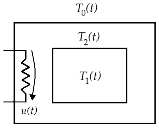
Figure 3.
Thermal plant scheme.
Based on the principle of conservation of energy, the equations describing the dynamics of the process can be deduced as
where and represent the masses of the specified media, and are the specific heat of the media, and and are the interfaces between mentioned rooms.
Using the relations in Equation (1), the system can be described in the input–state–output paradigm, using as state variables , the temperature in the inner room, the first state, and as the second state, resulting in
The assessment of control for temperature treatment systems using reference signals such as the cyclic quenching and stabilization–carbonization scenarios is performed using specific performances, such as those mentioned in [33]:
- -
- ramp error is measured at a certain time moment during the ramp, providing information on the accuracy with which the ramp reference is tracked; typical ramp error ;
- -
- bring-in measures the efficiency of the controller to turn the corner from ramp to soak, being defined as the area enclosed between the required setpoint trajectory shifted in time and the setpoint temperature at steady state;
- -
- overshoot: the corner of the setpoint trajectory should be turned minimal overshoot.
The performance of the model-free control laws will be evaluated for the proposed scenarios for the purpose of heat treatment based on these criteria. iPI-type control laws will be analyzed in a comparative manner to validate those presented in [24], but also to compare the iPI-IFT variant with the iPI-SMC one.
3. Design of the iPI Controllers
The iPID controllers use an ultra-local model based on which a controller parameter is estimated at each sampling time based on the process input and output signals acquired from the running control system. The behavior of these regulators can be assimilated to that of various structures of the classical PID depending on the order of the derivative of the output from the ultra-local model [3]. A special type of controller is iPI when the first derivative of the output is used, which has a PII2-type behavior with a double integrator. This kind of controller is suitable for situations where it is necessary to follow a ramp and soak reference with a minimum error, or when the output of the system is expressed as a derivative of another signal in the system.
The discrete time ultra-local model for an iPI controller, as [14] suggests, can be expressed as
where is used to obtain the first-order derivative using the backward difference approximation based on the Z transformation, with the sampling period . The discrete-time output of the system is , while represents the discrete-time control signal, is a parameter chosen by the practitioner, and is a discrete-time parameter used by the iPI controller defined by
where is the reference. The discrete-time PI controller embedded in iPI is
where and are the controller’s proportional and integral gains and is the control error.
The controller parameter in Equation (4) is estimated at each sampling time based on the ultralocal model (3), resulting in
According to Equations (4)–(6), the discrete-time control law of an iPI controller is found as
having a PII2-like behavior.
Assuming a good estimate of , introducing from Equation (4) into (3), after a few simple calculations, the following equation of the control error dynamics is obtained:
To obtain a zero steady-state error (i.e., ), the roots of the characteristic polynomial of the error
must be stable. Root stability can be analyzed by applying the Jury test based on the characteristic polynomial coefficients. Thus, based on the characteristic polynomial of the error (9), by applying the Jury test, the stability domain of the roots in the tuning parameters plane is obtained, defined by the inequalities [34]
In order to design the iPI controller in the following, we will present the use of the data-driven IFT algorithm for determining the tuning parameters, and a hybrid version obtained by adding an SMC component to the iPI control signal.
3.1. iPI-IFT Algorithm
The setting of the parameters for an iPI controller can be difficult, especially in the context where no clear rules are mentioned regarding their values. One way is stated in [24], where, based on the error equation and the Jury test, a domain is obtained in which the parameters can take values that ensure a zero steady-state error.
In [14], a method is specified for tuning the iPI controllers using a conjunction of the original MFC method with another data-driven method, IFT. The method defined by Hjalmarsson in [10] provides an algorithm by which the parameters of a control law can be improved by minimizing a cost function. Following the minimization, a set of optimal parameters of the controller is obtained, the method being one of improving the performance of the control law.
In order to tune the iPI controller with the IFT method, a controller with fixed structure is necessary, as specified in [10]. An approximation with a transfer function for the control law from Equation (6) may be obtained by applying the Z transform to it, which leads to
with the following tuning parameters grouped in the vector :
The tracking error depending on the vector parameter is defined as
where represents the output of the system after using the set of parameters for the controller.
The design objective is imposed as a quadratic function defined by
where is the control signal for the used set of parameters and is the tracking error using the same set of parameters . and are filters that weighted the output and control signals, is a penalty factor, and N is the number of samples. The cost function from Equation (14) will be minimized by the following optimal parameter vector:
To obtain the minimum, which the optimal parameter set provides, it is necessary to minimize the derivative of . For simplicity, the values of and are taken to be equal to 1, and the derivative of becomes
The gradient of can be calculated based on Equation (16), while the optimal parameters may be obtained in an iterative way using
where is a positive real scalar that determines the step size, while is a symmetric positive defined matrix used to update the direction. This matrix can be considered the identity matrix, or it can be defined as [10] mentions as
Because the value of the gradient in Equation (14) is unknown, it must be estimated, . For this, it is necessary for the data acquisition of the tracking error and the control signal , which will be used to compute the estimation of gradients and . Those will lead to the unbiased estimation of the products and . These signals are acquired following closed-loop experiments, using the controller defined by Equation (11), with the parameters .
Therefore, using Equation (13), we can conclude that
which shows us that the previously mentioned gradient estimates refer to the control and output signals of the system. The derivatives of the control and output signals obtained for the parameter set can be obtained using the relations
where represents the closed loop transfer function of the system, while is the sensitivity function, as [10] suggests. According to the same source, the derivatives will be calculated for each step , knowing the transfer function of the controller, with the related parameter set, . This step will be repeated in an algorithm with two sets of experiments of equal length, . The first experiment, , provides for the excitation of the system with reference , resulting in
while the second experiment, , provides a reference represented by the difference between the original reference and the response of the system to the first experiment, . The signals obtained are:
The signals obtained in each of the two experimental sets are denoted by superscripts and .
The relations for estimating the gradients are proposed in [10] as
Using the estimates in Equation (23), an estimate of the derivative of the cost function for the current parameter set , , can be found as
A similar estimate using the data from the two mentioned experiments can be obtained for the matrix , from Equation (18), as follows
The set of parameters , will result in an iterative manner, based on using Equation (24), along with Equation (25) as
The applicable IFT algorithm for the iPI regulation law will have the following steps:
- For the first iteration , the reference will be applied to the control system, in the context of using a set of parameters obtained applying the Jury test to the characteristic polynomial of control error [24], which will ensure a stable response for the control system.
- Following the first experiment, the input , output , and tracking error signals are acquired.
- The set of parameters obtained in the previous iteration will be used for an atypical experiment, where the reference signal will be . Following the application of this reference, the input , output , and tracking error signals will be acquired, based on which the criterion will be minimized, and a new set of parameters will be obtained.
- The sequence of experiments of type , typical reference, and , augmented reference, is repeated, until the desired performances are fulfilled. At that point, it is considered that an optimal set of parameters is reached for the tuning law, and the algorithm terminates. The flowchart of the algorithm is depicted in Figure 4.
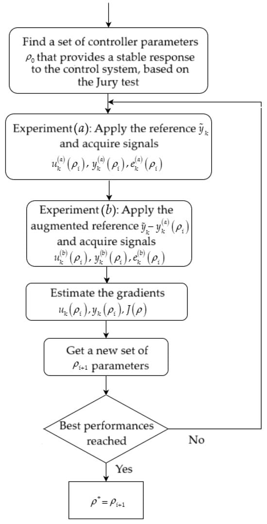 Figure 4. Flowchart representation of the iPI-IFT algorithm.
Taking into account the methods proposed for the calculation of , the iPI-IFT algorithm was applied twice, resulting in a set of parameters for the variant, in which is the identity matrix, hereafter referred to as iPI-IFT1, and a set for the situation in which is obtained according to Equation (25), being called iPI-IFT2.
3.2. iPI-SMC Algorithm
The SMC algorithm can be used in conjunction with an iPI-type MFC law, as is introduced in [18], considering the continuous-time variant of the resulting algorithm iPI-SMC. Using the ultra-local model (3) and the iPI algorithm (4), written in a continuous-time paradigm, an augmented component is added, resulting in
is estimated using the ultra-local model
where is the first-order derivative approximation, usually with a filtered derivative element. Substituting from Equation (28) into (27), and considering the estimation error , results in the dynamics of the control error of the control system with the iPI-SMC controller:
To realize the conjunction between the iPI law and the SMC, the following states need to be considered:
and thus, the state equations of control system are obtained using Equation (30)
For the design of the sliding mode law, the switching variable will be used as
where is the parameter which designs the behavior of the system on the sliding surface. The stability of the system in closed loop is ensured by the Lyapunov function as follows:
Based on the Lyapunov stability theory, the existence condition and sliding mode reaching is obtained by as
which is employed to derive the control law , based on and , as [18] suggests. The derivative of may be expressed as
Using the state Equation (31) in Equation (35) will result in the derivative of as
The augmented control law in Equation (27) has the following two components: an equivalent control signal and a correction control signal [18]:
The equivalent component is obtained in the ideal sliding mode condition , which leads to .
By inserting Equation (37) into Equation (36), with and solving for , it will result in
where the estimation error can be bounded to a maximum value , as .
In order to satisfy the condition of the existence of the sliding surface, as well as to reduce the chattering effect, a boundary layer is applied. The expression of the is
where and are the convergence factor and the boundary layer thickness, respectively.
Following Theorem 1 from [18], the augmented control signal can be written as
The iPI-SMC control law results by inserting Equation (40) in Equation (27) as
The discrete-time form of Equation (41) becomes
Thus, the iPI-SMC law becomes one dependent on the tuning parameters , the parameter chosen by the practitioner as [3] mentions, and is a design parameter that will be chosen by testing, like the convergence factor and the boundary layer thickness. In addition, will be calculated according to Equation (6) and , and will be considered to have a very small value.
4. Comparison of the iPI Controllers Used for the Heating Treatment Process
In order to highlight and analyze the behavior of the laws described in Section 3, the temperature profiles described in detail in Section 2 were considered. The parameters for the system described by Equation (2) are those proposed in [35] as follows: For each, the specific performances presented in Section 2 were analyzed, but the tuning errors were also calculated using specific criteria.
For the tuning of the iPI controller, in its initial version named iPI0, the stability domain offered by the Jury test (10) was used, so that the set of parameters would be the starting point for the iPI-IFT1-2 laws. The iPI laws and variants granted by IFT will be compared with an iPI-SMC law, described in Section 3.2, to compare which of the variants has better performance and smaller tuning errors, which is a vital element in heat treatments that require high precision regarding tracking the temperature reference.
Starting from the iPI0 controller parameters that stabilize the system, obtained by the previously mentioned method, the IFT method was applied using the two calculation types of the matrix. For the first case, seven complete iterations of the iPI-IFT1 algorithm were performed, and the values of the cost function that had to be minimized are shown in Figure 5.
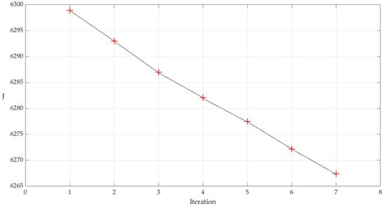
Figure 5.
Graphical representation of the variation during iPI-IFT1.
Using the same set of starting parameters, six complete iterations of the iPI-IFT2 algorithm were performed using the variant described in Equation (25) to calculate . The values obtained for are those in Figure 6.
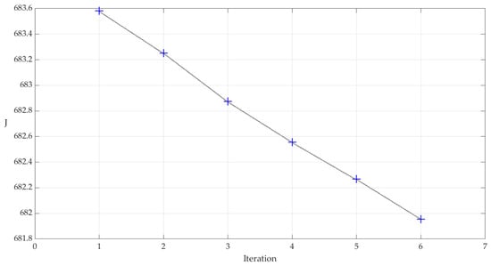
Figure 6.
Graphical representation of the variation during iPI-IFT2.
As Figure 5 and Figure 6 show, the values of are minimized following the iterative process applied to the iPI law. Comparing the two graphs, it can be seen that the values for the case where the matrix defined by (25) is used are an order of magnitude 10 times smaller than when the unit matrix is used for the calculation of the optimal parameter set.
The optimal parameter set of iPI-IFT1 is
While the optimal parameter set for iPI-IFT2 is
4.1. Cyclic Quenching Scenario
The quenching scenario consists of four temperature increases and decreases between room temperature and 810 °C, as detailed in Section 2.
For this simulation scenario, the results of the following four iPI-type control laws were compared: iPI0, iPI-IFT1, iPI-IFT2, and iPI-SMC. The results are shown in Figure 7.
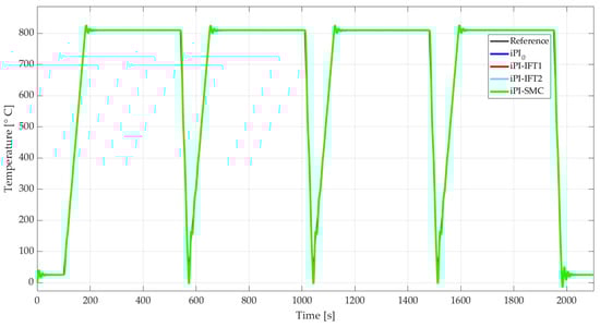
Figure 7.
System outputs for the quenching scenario.
It can be seen that all four laws track the reference signal, which has slopes of 10 °C per second, situations for which a double-integral component is required. Details of Figure 7 can be seen in Figure 8 and Figure 9.
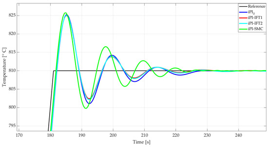
Figure 8.
System outputs for the quenching scenario—detailed view 1.
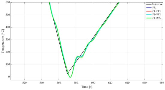
Figure 9.
System outputs for the quenching scenario—detailed view 2.
The control signals represented by the power of the thermal system for the quenching scenario are represented in Figure 10. It can be seen that the values are relatively similar, having very small variations from each other.
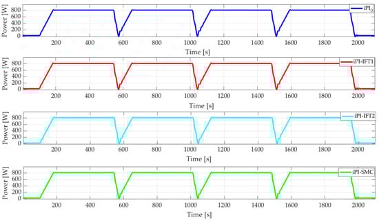
Figure 10.
Control signals for the quenching scenario.
The control errors for the quenching scenario can be observed in Figure 11. It can be seen how, after reaching the ambient temperature of 25 °C, starting with the reference from 0, the biggest errors appear when the ramp turns from negative to positive values. Those are the times when the system needs a few seconds to successfully track the reference. As can be seen from the graph, the error is cleared quickly, with the system returning within reasonable limits of the error level. A detailed view is depicted in Figure 12.
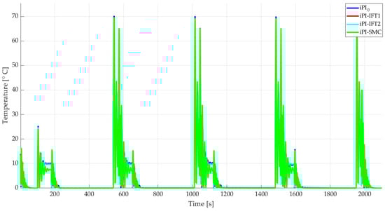
Figure 11.
Control errors for the quenching scenario.
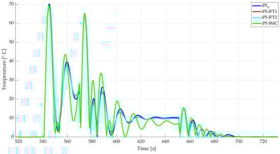
Figure 12.
Control errors for the quenching scenario—detailed view.
4.2. Carbonization–Stabilization Scenario
The second type of simulated thermal treatment is that applied to carbon membranes, which provides for the following two phases: stabilization and carbonization. Thus, the reference applied in such a process has a slower variation compared to cyclic quenching from the first scenario. The increase in temperature up to 350 °C is achieved at a rate of 3 degrees per second, after which the temperature is maintained for 30 min. After the stabilization at the temperature of 350 °C is achieved, a new increase follows with the same rate up to 700 °C, and the temperature is maintained for another 30 min. Finally, the temperature is reduced to the ambient value. The system outputs for the four proposed iPI-type control laws are shown in Figure 13.
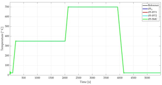
Figure 13.
System outputs for the stabilization–carbonization scenario.
A detailed view for the stabilization–carbonization scenario is shown in Figure 14.
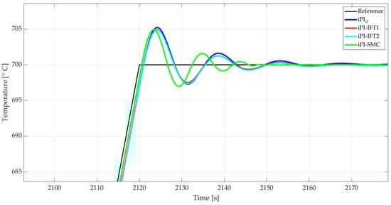
Figure 14.
System outputs for the stabilization–carbonization scenario—detailed view.
For the four proposed laws, the control quantity, represented by the power required to heat the interior, is depicted in Figure 15.
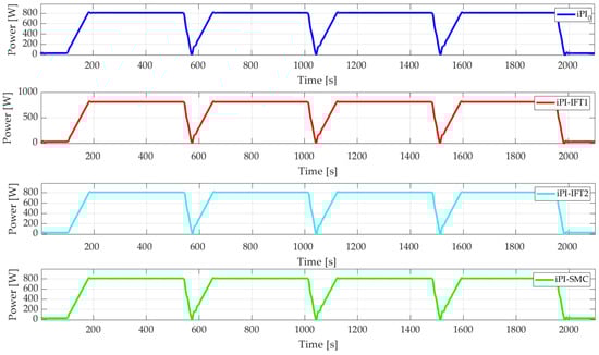
Figure 15.
System control signals for the stabilization–carbonization scenario—zoom.
The control errors, represented by the difference between the reference values and the temperatures measured in the inner room, are represented in Figure 16.
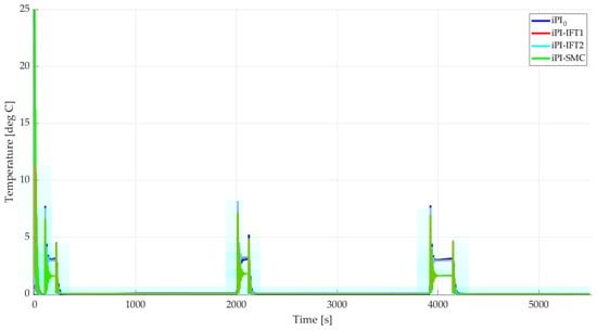
Figure 16.
Control error signals for the stabilization–carbonization scenario.
It can be seen from Figure 16 that the biggest error occurs at the beginning of the process when the temperature of the indoor environment reaches from 0 °C to the value considered for the ambient environment of 25 °C. Subsequently, throughout the stabilization–carbonization scenario, the errors are below 10 °C. A detailed view of how the error varies for the stabilization phase can be seen in Figure 17.
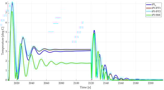
Figure 17.
Control error signals for the stabilization phase—detailed view.
4.3. Performance Analysis
Performance analysis for heat treatment systems may be slightly different from classic control systems. This is because, as mentioned in Section 2, such systems have a reference consisting of ramps, followed by a temperature holding period. Thus, ref. [33] the three performances for evaluating systems responses under such circumstances as defined in Section 2 are used.
Based on these three performances, the two control scenarios with the four iPI laws described in Section 3 were analyzed. The results for the first scenario are shown in Table 1 and for the second scenario in Table 2. Transient performances were analyzed for ramp ascent and descent approaches from described scenarios. “Mean” represents the average value of the absolute error, calculated over the entire duration of the considered ramp, while “Max” represents the absolute maximum value of the error for the same ramp.

Table 1.
Performance analysis for the quenching scenario.
Table 2.
Performance analysis for the second scenario.
In the case of the first scenario, for ramp error, both when ascending and when descending, the performances are significantly equal between the original variant and the two variants with IFT, while the SMC variant has an advantage. Also, the maximum variation from the reference value is maintained within a window of 25 °C. In the descending part, high values of the maxima compared to the reference are observed, at the moment of the change from the descending to the ascending area, which is also highlighted by Figure 5 and Figure 7. After these moments, the error reaches small values, which make the average either around 1.55 °C for the iPI0 and iPI-IFT variants, while for iPI-SMC, the average deviation is 1.37 °C. The values for bring-in are relatively similar, while the overregulation is lower in the initial version of iPI0 compared to IFT and SMC.
From Table 1 and Table 2, an improvement in the performance can be seen by applying IFT in both calculation versions of the matrix, compared to the original version; however, the best performances were obtained for the iPI-SMC variant.
In the case of the second scenario, much lower average values can be observed, compared to the first, both on the ascending zone between 2000 and 2120 s, and on the descending zone between 3920 and 4120 s. This is mainly due to the slope of only 5 °C per minute, compared to 10 °C per minute in the first scenario. Moreover, the maximum difference throughout the rise and fall is kept below 9 °C, the bring-in duration being relatively similar, with a small advantage for the SMC variant, while the overshoot values are equal, with a small disadvantage for the initial iPI0.
Overall, from the analysis of the two tables, a slight improvement can be observed by using the two variants of IFT applied to the iPI law, but the best results are obtained by the iPI-SMC method.
In addition to the specific performances of heat treatment systems, mentioned in [26], the classical comparison criteria applied in [24] were also applied, to observe if the performance trend is respected in this situation. The reference tracking accuracy during the simulation of the two scenarios S1 and S2, in addition to the performance analysis previously presented in Table 1 and Table 2, the ISE and IAE criteria, were applied.
For ISE, the following formula was used:
And for the IAE criterion, the following formula was used:
The results for the two criteria, applied to the scenarios described in Section 2, are presented in Table 3.
Table 3.
Numerical analysis based on the ISE and IAE criteria.
The numerical analysis using the ISE and IAE criteria shows a decrease in the value of the errors, both quadratic and absolute, in both scenarios, after applying the two calculation variants of the matrix, for the iPI-IFT algorithm. The iPI-SMC law shows the smallest error values, as can be seen in both scenarios. The conclusions obtained through the analysis of Table 1 and Table 2 are confirmed based on the numerical analysis, as well as the results of the minimization of , shown in Figure 5 and Figure 6.
5. Conclusions
This paper proposed the analysis of some model-free control methods for heating treatment systems. Since such systems require gradual heating of the inner room, where the treatment is applied, various variants of the iPI controller were tested in a comparative manner, using two simulation scenarios. The first scenario consisted of a variant of cyclic quenching, where the temperature reference varied more rapidly, rising and falling at a rate of 10 °C per second. The second scenario was one of stabilization–carbonization, in which temperature variations were slower, the rate of increase being only 3 °C per second. The iPI-type control laws have been shown to be feasible for such applications, where the reference variations are a ramp–soak type. The performances analyzed for such variations, less common in the control domain, confirmed the expectations of these two integral-component control laws. Such a controller proves that it provides not only a steady-state error, but also a minimum error during the ramp variation.
Following the simulations carried out for the cyclic quenching scenario, it can be concluded that the desired performances were achieved by the analyzed control laws. The iPI-IFT variants provide improved outputs compared to the original variant, obtained based on the Jury test. The iPI-SMC law provided the best results in this scenario, both for the defined specific performances and from the numerical analysis.
Regarding the stabilization–carbonization scenario, the conclusions are similar to those of the cyclic quenching scenario, and it should be emphasized that the errors are much smaller in the situations where the growth rate is 3 °C per second, compared to 10 °C/s. Also, the overshooting and bring-in duration are superior in such a scenario. Also, in this scenario, the best results were obtained by the iPI-SMC law.
Regarding the use of the IFT algorithm applied to the iPI law, it can be found that it brings a benefit, both in what identified the errors and the dynamic performances. Following the results obtained, it can be concluded that for the calculation of the matrix, the computational effort required to use the calculation equation proposed by Hjalmarsson is not worth it, compared to the use of the identity matrix to obtain a new set of controller parameters.
For both simulation scenarios, it was found that the iPI-SMC law provides the best performance, both dynamically and from the perspective of the analyzed errors. Thus, the use of a sliding mode, which simplifies the tuning based on the and parameters, proves to be more effective in such applications, keeping the basic characteristics of a double-integrator law. But, in general, the iPI-type control laws prove to be useful for such applications in the field of heating treatment process.
Considering that the MFC is not based on a process model, for a better interaction with the environment and thus obtaining an improvement in performance, model-free reinforcement learning algorithms will be considered for future research.
Author Contributions
Conceptualization and methodology, C.L. and A.B.; software, A.B.; validation, formal analysis, investigation, resources, writing—original draft preparation, data curation, and investigation, A.B. and C.L.; writing—review and editing, visualization, supervision, and project administration, C.L. and A.B. All authors have read and agreed to the published version of the manuscript.
Funding
This research received no external funding.
Data Availability Statement
Data available from the authors upon request.
Conflicts of Interest
The authors declare no conflicts of interest.
References
- Hou, Z.-S.; Wang, Z. From model-based control to data-driven control: Survey, classification and perspective. Inf. Sci. 2013, 235, 3–35. [Google Scholar] [CrossRef]
- Hou, Z.; Chi, R.; Gao, H. An Overview of Dynamic-Linearization-Based Data-Driven Control and Applications. IEEE Trans. Ind. Electron. 2016, 64, 4076–4090. [Google Scholar] [CrossRef]
- Fliess, M.; Join, C. Model free control. Int. J. Control. 2013, 86, 2228–2252. [Google Scholar] [CrossRef]
- La Hera, P.; Mendoza-Trejo, O.; Lideskog, H.; Morales, D.O. A framework to develop and test a model-free motion control system for a forestry crane. Biomim. Intell. Robot. 2023, 3, 100133. [Google Scholar] [CrossRef]
- Precup, R.-E.; Roman, R.-C.; Teban, T.-A.; Albu, A.; Petriu, E.M.; Pozna, C. Model-Free Control of Finger Dynamics in Prosthetic Hand Myoelectric-based Control Systems. Stud. Inform. Control 2020, 29, 399–410. [Google Scholar] [CrossRef]
- Hegedus, T.; Fenyes, D.; Nemeth, B.; Szabo, Z.; Gaspar, P. Design of Model Free Control with tuning method on ultra-local model for lateral vehicle control purposes. In Proceedings of the 2022 American Control Conference (ACC), Atlanta, GA, USA, 8–10 June 2022. [Google Scholar]
- Villagra, J.; Join, C.; Haber, R.; Fliess, M. Model-free control for machine tools. arXiv 2020, arXiv:2005.08546. [Google Scholar]
- Liu, Y.; Yan, W.; Xu, D.; Yang, W.; Zhang, W. Direct Torque Control of PMSM Based on Model Free iPI Controller. In Proceedings of the 2018 IEEE 7th Data Driven Control and Learning Systems Conference (DDCLS), Enshi, China, 25–27 May 2018; pp. 970–973. [Google Scholar]
- MohammadRidha, T.; Ait-Ahmed, M.; Chaillous, L.; Krempf, M.; Guilhem, I.; Poirier, J.-Y.; Moog, C.H. Model Free iPID Control for Glycemia Regulation of Type-1 Diabetes. IEEE Trans. Biomed. Eng. 2018, 65, 199–206. [Google Scholar] [CrossRef]
- Hjalmarsson, H.; Gevers, M.; Gunnarsson, S.; Lequin, O. Iterative feedback tuning: Theory and applications. IEEE Control. Syst. Mag. 1998, 18, 26–41. [Google Scholar] [CrossRef]
- Lequin, O.; Gevers, M.; Mossberg, M.; Bosmans, E.; Triest, L. Iterative feedback tuning of PID parameters: Comparison with classical tuning rules. Control. Eng. Pr. 2003, 11, 1023–1033. [Google Scholar] [CrossRef]
- Procházka, H.; Gevers, M.; Anderson, B.D.; Ferrera, C. Iterative feedback tuning for robust controller design and optimization. In Proceedings of the 44th IEEE Conference on Decision and Control, Seville, Spain, 15 December 2005; pp. 3602–3607. [Google Scholar]
- Gonzalez-Villagomez, J.; Rodriguez-Donate, C.; Lopez-Ramirez, M.; Mata-Chavez, R.I.; Palillero-Sandoval, O. Novel Iterative Feedback Tuning Method Based on Overshoot and Settling Time with Fuzzy Logic. Processes 2023, 11, 694. [Google Scholar] [CrossRef]
- Baciu, A.; Lazar, C. Iterative Feedback Tuning of Model-Free Intelligent PID Controllers. Actuators 2023, 12, 56. [Google Scholar] [CrossRef]
- Novaes Menezes, E.J.; Araújo, A.M.; da Silva, N.S.B. A review on wind turbine control and its associated methods. J. Clean. Prod. 2018, 174, 945–953. [Google Scholar] [CrossRef]
- Hossain, A.; Islam, R.; Hossain, A.; Hossain, M.J. Control strategy review for hydrogen-renewable energy power system. J. Energy Storage 2023, 72, 108170. [Google Scholar] [CrossRef]
- Li, G.; Wang, X.; Liang, B.; Li, X.; Zhang, B.; Zou, Y. Modeling and control of nuclear reactor cores for electricity generation: A review of advanced technologies. Renew. Sustain. Energy Rev. 2016, 60, 116–128. [Google Scholar] [CrossRef]
- Precup, R.-E.; Radac, M.-B.; Roman, R.-C. Model-free sliding mode control of nonlinear systems: Algorithms and experi-ments. Inf. Sci. 2017, 381, 176–192. [Google Scholar] [CrossRef]
- Precup, R.-E.; Roman, R.-C.; Safaei, A. Data-Driven Model-Free Controllers, 1st ed.; Taylor & Francis: London, UK, 2021. [Google Scholar]
- Gao, P.; Lv, X.; Ouyang, H.M.; Mei, L.; Zhang, G.M. A novel model-free intelligent proportional-integral super twisting nonlinear fractional-order sliding mode control of PMSM speed regulation system. Complexity 2020, 2020, 8405453. [Google Scholar] [CrossRef]
- Gao, P.; Zhang, G.; Lv, X. Model-Free Hybrid Control with Intelligent Proportional Integral and Super-Twisting Sliding Mode Control of PMSM Drives. Electronics 2020, 9, 1427. [Google Scholar] [CrossRef]
- Zhu, Q.; Li, R.; Zhang, J. Model-free robust decoupling control of nonlinear nonaffine dynamic systems. Int. J. Syst. Sci. 2023, 54, 2590–2607. [Google Scholar] [CrossRef]
- nen, Ü. Model-Free Controller Design for Nonlinear Underactuated Systems with Uncertainties and Disturbances by Using Extended State Observer Based Chattering-Free Sliding Mode Control. IEEE Access 2023, 11, 2875–2885. [Google Scholar]
- Baciu, A.; Lazar, C.; Caruntu, C.-F. Iterative Feedback Tuning of Model-Free Controllers. In Proceedings of the 25th International Conference on System Theory, Control and Computing (ICSTCC), Iasi, Romania, 20–23 October 2021; pp. 467–472. [Google Scholar]
- Tong, Y.; Zhang, Y.-Q.; Zhao, J.; Quan, G.-Z.; Xiong, W. Wear-Resistance Improvement of 65Mn Low-Alloy Steel through Adjusting Grain Refinement by Cyclic Heat Treatment. Materials 2021, 14, 7636. [Google Scholar] [CrossRef]
- Ismail, N.H.; Salleh, W.N.W.; Sazali, N.; Ismail, A.F. Effect of intermediate layer on gas separation performance of disk supported carbon membrane. Sep. Sci. Technol. 2017, 52, 2137–2149. [Google Scholar] [CrossRef]
- Gokhman, A.; Nový, Z.; Salvetr, P.; Ryukhtin, V.; Strunz, P.; Motyčka, P.; Zmeko, J.; Kotous, J. Effects of Silicon, Chromium, and Copper on Kinetic Parameters of Precipitation during Tempering of Medium Carbon Steels. Materials 2021, 14, 1445. [Google Scholar] [CrossRef] [PubMed]
- Delahaigue, J.; Chatelain, J.-F.; Lebrun, G. Influence of Cutting Temperature on the Tensile Strength of a Carbon Fiber-Reinforced Polymer. Fibers 2017, 5, 46. [Google Scholar] [CrossRef]
- Gustav, K.; Åhag, L. An AI Approach for Quality Improvement in Heat Treatment Processing. Master’s Dissertation, Uppsala Universitet, Uppsala, Sweden, 2022. [Google Scholar]
- Antonescu, I.; Alecu, C.I.; Lepadatu, D. Advanced systems for heat treatment controlling of electrical furnaces. IOP Conf. Ser. Mater. Sci. Eng. 2019, 485, 012002. [Google Scholar] [CrossRef]
- Yang, J.; Feng, B. Intelligent Control System of Metal Surface Heat Treatment Based on Fuzzy PID Technology. In Proceedings of the 2023 IEEE International Conference on Control, Electronics and Computer Technology (ICCECT), Jilin, China; 2023; pp. 1354–1358. [Google Scholar]
- Li, J.; Wei, H.; Wu, H.; Li, Y. Research on Heat Treatment Control Technology of Machining Parts. Procedia Eng. 2011, 15, 173–177. [Google Scholar] [CrossRef][Green Version]
- Balakrishnan, K.; Edgar, T. Model-based control in rapid thermal processing. Thin Solid Films 2000, 365, 322–333. [Google Scholar] [CrossRef]
- Jury, E.I. Theory and Application of the z Transform Method; Wiley: New York, NY, USA, 1964. [Google Scholar]
- Jacquot, R.G. Modern Digital Control Systems, 2nd ed.; Taylor & Francis: London, UK, 2019. [Google Scholar]


Disclaimer/Publisher’s Note: The statements, opinions and data contained in all publications are solely those of the individual author(s) and contributor(s) and not of MDPI and/or the editor(s). MDPI and/or the editor(s) disclaim responsibility for any injury to people or property resulting from any ideas, methods, instructions or products referred to in the content. |
© 2024 by the authors. Licensee MDPI, Basel, Switzerland. This article is an open access article distributed under the terms and conditions of the Creative Commons Attribution (CC BY) license (https://creativecommons.org/licenses/by/4.0/).