Article

Multivariable Control-Based dq Decoupling in Voltage and Current Control Loops for Enhanced Transient Response and Power Delivery in Microgrids

by
Mandarapu Srikanth
1,
Yellapragada Venkata Pavan Kumar
1,*,
Challa Pradeep Reddy
2 and
Rammohan Mallipeddi
3,4,*
1
School of Electronics Engineering, VIT-AP University, Amaravati 522237, Andhra Pradesh, India
2
School of Computer Science and Engineering, VIT-AP University, Amaravati 522237, Andhra Pradesh, India
3
Department of Artificial Intelligence, School of Electronics Engineering, Kyungpook National University, Daegu 37224, Republic of Korea
4
Smart Agriculture Innovation Center, Kyungpook National University, Daehak-Ro 80, Daegu 41566, Republic of Korea
*
Authors to whom correspondence should be addressed.
Energies 2024, 17(15), 3689; https://doi.org/10.3390/en17153689
Submission received: 19 April 2024 / Revised: 26 June 2024 / Accepted: 22 July 2024 / Published: 26 July 2024
(This article belongs to the Special Issue Power Quality and Hosting Capacity in the Microgrids)

Abstract

:
Being multivariable in nature, voltage and current control loops have controllers in the forward and cross-coupling paths. Most methods discussed in the literature focus on tuning the controllers in the forward paths to reduce the dq coupling. A modified pole-zero cancellation (MPZC) technique has recently been discussed, which uses the concepts of pole-zero cancellation and particle swarm optimization to effectively tune the forward path controllers. However, given the fixed gains in the cross-coupling paths, it is not possible to realize a superior transient response from this technique. Therefore, to achieve enhanced vector control of VSIs under transient conditions, this paper proposes a hybrid MPZC (HMPZC) method, which incorporates multivariable control along with the MPZC technique for both voltage/current control loops. In the proposed HMPZC method, the MPZC method is used to tune the forward path controllers, and multivariable control-based PI controllers are assigned in the cross-coupling paths of dq-axes loops rather than fixed gains. In this paper, these multivariable control-based PI controllers are designed using direct synthesis method-based internal model control (IMC). From the simulation results, it is verified that the proposed HMPZC method has reduced the coupling between the d- and q-axes loops of the current/voltage, leading to the improved transient response and power delivery capability of VSIs.

1. Introduction

The primary objective of microgrids is to deliver the required active power (P) and reactive power (Q), while maintaining the voltage and frequency. The guidelines to attain these objectives are based on the IEEE 1547-2018 standard [1]. Most of the DERs in microgrids are driven by power electronic converters. Voltage source inverters (VSIs) are a common type of power electronic converter to interface with the DERs in AC microgrids. VSIs with proper control help (i) in achieving a better transient response, i.e., maintaining the voltage and frequency within limits, and (ii) in improving stability by achieving a better power-handling capability. A VSI with a power–voltage–current control structure which allows operation in off-grid and grid-tied modes is chosen for the proposed work in this paper. The role of the power controller is vital in upholding the stability of the system (power-handling capability) under sudden power demands (transient conditions). A conventional droop control-based power controller regulates the P through the active power loop (APL), which is based on P-ω droop control logic. Similarly, Q is regulated through the reactive power loop (RPL), which is based on Q-v droop control logic [2]. The major limitation of this conventional droop control is its operation during islanded mode. The impact of power demands on the movement of low-frequency dominating modes and the impact of droop gains in ensuring system stability are discussed in [3]. It is identified in [4] that adaptive droop control, rather than fixed droop, enhances the transient response/stability. The proposed method in this paper deploys adaptive droop control for the power controller.
The multivariable nature of VSIs, which causes the coupling between the P and Q, is a major cause of poor power-handling capability and transient response with VSIs, especially under an islanded mode of operation and transient conditions [5]. Several methods were discussed in the literature that focused on reducing the coupling in multivariable control systems [6,7]. From this, it is understood that two possible approaches are available in the literature which can reduce the coupling. These approaches are based on trying to decouple the (i) APL and RPL of the power controller and (ii) the d- and q-axes loops of inner control loops. In the direction of the first approach, the most generic way of reducing the coupling between the APL and RPL of the power controller is achieved by introducing a virtual impedance loop [8,9]. Recently, a multivariable controller-based decoupling of the APL and RPL of power controllers has been discussed in [10]. However, the dynamics of either the virtual impedance loop or power loop are slower than the dynamics of the inner voltage control loop (VCL) and current control loop (CCL). Thus, the VCL and CCL can significantly impact the transient response and power-handling capability [11]. This provided the necessary motivation for the authors to take up a second approach to modify the inner VCL and CCL. Moreover, as far as the authors are aware, the scope of the inner VCL and CCL in providing a decoupled control of P and Q has not been explored.
The necessary background and developments connected with the second approach are described as follows. The vector control of the VSI allows a decoupled control of active and reactive powers in a steady state [12]. P is regulated by the d-axis components of the output voltage and output current, while Q is regulated by the d-axis component of the output voltage and q-axis component of the output current. This signifies the role of the VCL and CCL in providing a decoupled control of P and Q and thereby in the power-handling capacity of the power controller [13]. An analytical representation of a VSI in dq coordinates in relation to the AC and load dynamics identifies the multivariable (multi-input multi-output) nature of VSIs with reference to the inner voltage and current controllers [14]. Even though vector control of VSIs provides a decoupled control under a steady state, the presence of an LC filter causes an increased coupling between the dq loops of the VCL and CCL under transient conditions. This leads to poor transient response and limited power-handling capability [15].
Being multivariable in nature, the VCL and CCL have controllers in the forward and cross-coupling paths. Most methods discussed in the literature focus on tuning the controllers in the forward paths to reduce the dq coupling. Internal model control (IMC)-based methods of tuning the voltage and current controllers are discussed in [16]. However, the presence of a derivative in the controller of the forward path hampers the applicability of this scheme [17]. The pole-zero cancellation-based method of tuning the voltage and current controllers does not require a derivative in the controllers and so can address this drawback. However, as the voltage controller’s integral gain in this method is fixed to zero, the advantage of this technique under transient conditions is limited [18]. To address this issue and achieve a better controller in the forward paths of both the VCL and CCL, a modified pole-zero cancellation method (MPZC) is presented in [19]. Here, the integral coefficient of the voltage controller is tuned with particle swarm optimization to replace the zero value of the integral coefficient with a more reliable value. However, this method suffers from fixed gains in the cross-coupling paths which cannot provide a better decoupling, especially under transients. Therefore, a better decoupling can be achieved by employing multivariable control rather than focusing only on tuning the controllers in the forward paths. The description provided in Section 3.5 justifies the limitations of MPZC and the effect of coupling.
The method of providing decoupling in VSIs by introducing a separate decoupler whose inputs are tuned through PID controllers in the feed-forward paths is discussed in [20]. The design of these decouplers for VSIs, which are mainly based on predictive control, is widely discussed in the literature [21,22]. Even though a good performance can be achieved, these decouplers increase the complexity of the control structure and the computational burden [23]. Thus, this paper employs the other way of providing multivariable control, without the need for a separate decoupler. Conventionally, in this method, the coupling terms are used as feed-forward signals to nullify the coupling effect [24]. However, this requires the exact determination of the coupling terms, which is commonly impossible [25]. So, this kind of multivariable control approach of VSIs is not effective, especially during transient conditions. This method of multivariable control is equivalent to introducing simple proportional gains in the cross-coupling paths, which cannot address steady-state error issues effectively [26]. To reduce the steady-state error effects that may occur due to an improper estimation of terms in the cross-coupling paths, the literature has suggested introducing a simple integrator in cross-coupling paths [27,28]. However, the tuning of the integral gains of the cross-coupling paths may not be easy and straightforward. Further, a simple integrator may not be sufficient in enhancing the performance of a VSI’s vector control under transient conditions [29].
Based on the summary of the aforesaid literature review, the identification of the research gap and its solution in the form of the proposed method is described as follows. Several PID tuning methods were discussed in the literature to provide decoupling in multivariable control [30,31,32,33,34,35,36]. These methods can be used for the design of controllers in the cross-coupling paths. However, a better transient response cannot be expected if the design of these controllers is carried out by neglecting a dynamic model of VSIs. Amongst various methods discussed in the literature to provide decoupling from cross-coupling paths, IMC control is popular as this takes the system model into account for its implementation [33,34,35,36]. The synthesis of IMC in these works is accomplished with triangular decoupling [33], inverted decoupling [34], fractional order models [35], and direct synthesis [36]. However, the procedure described [33,34,35] for the design of IMC-based controllers in cross-coupling paths is complex for application to the VCL and CCL. This is because the plant model considered in the design of the VCL and CCL for VSIs is the minimum phase. The direct synthesis procedure [36] of deriving the IMC-based controller for a typical feedback control system that is discussed in [37] offers a reduced complexity that is more compatible with the VCL and CCL. Therefore, to achieve the reduced coupling, improved transient response, and increased power-handling capability of microgrids, this paper proposes a hybrid MPZC method for the VCL and CCL. Here, the MPZC method is used to tune the forward path controllers, and an IMC-based multivariable control designed with a direct synthesis method is adopted for the design of controllers in the cross-coupling paths. As far as the authors are aware, the proposed method in the context of VCL and CCL is not yet explored in the literature.
The subsequent sections of this article are structured in the following manner. In Section 2, an analytical representation of the studied microgrid is discussed. Further, the problem identification, followed by the proposed solution, is also discussed in this section. Section 3 discusses the mathematical background and implementation of the proposed methodology in depth. Based on the results obtained from a simulation conducted in MATLAB (9.9)/Simulink (10.2) of R2020b software, the performance of the proposed and the conventional schemes are discussed in Section 4. In Section 5, the conclusion of this work is presented, based on the salient outcomes of the proposed research.

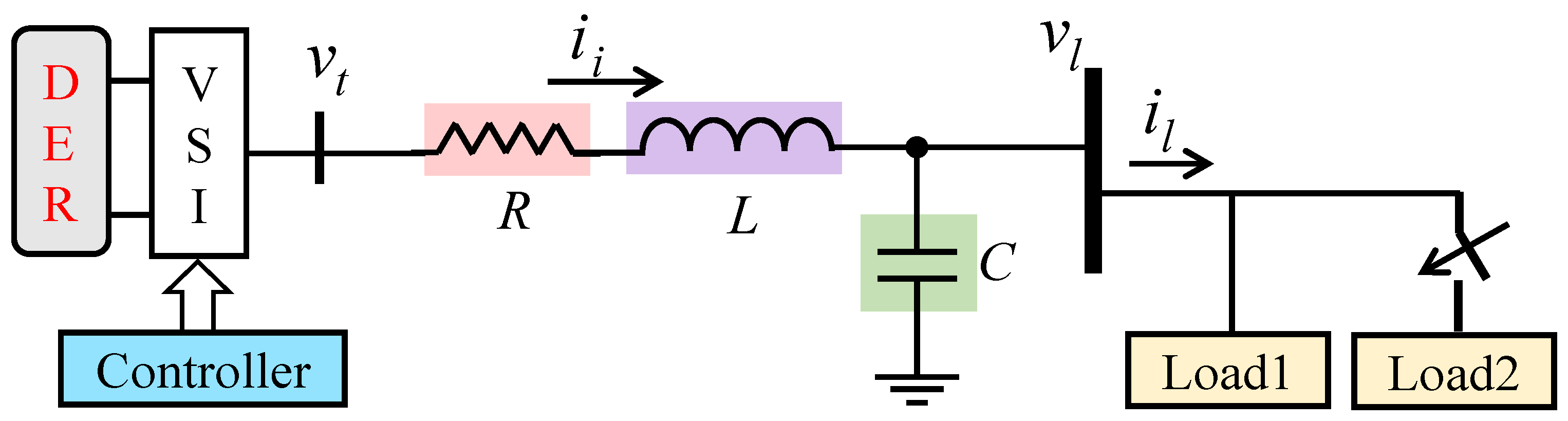
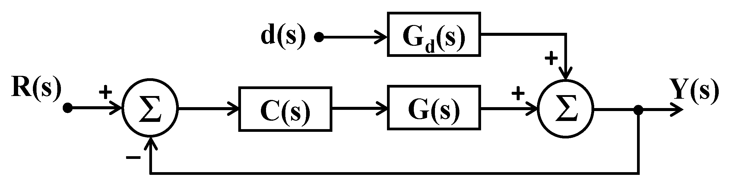
2. Mathematical Model of VSI and MPZC Description

A layout diagram representing the investigated three-phase AC microgrid model is shown in Figure 1. The model is driven by a DER of 25 kW + j25 kVar capacity. The DER’s output DC voltage (540 V rated) is inverted to AC by a VSI which acts as an interface between the DER and the loads. An LC filter is provided on the AC side of the VSI, whose ratings are given as R = 0.1 mohm, L = 1 mH, and C = 5 μF, where R is the associated resistance of the filter inductor. Two loads are connected to the system after the LC filter. Load1 draws the power from the system continuously, and load2 draws the power momentarily, as long as the associated breaker is kept on. With the help of the controller, the VSI regulates the power, voltage, and current that are supplied to the load.
An outline of the multiloop control structure that is employed in this work for the studied microgrid is depicted in Figure 2. In this control structure, the VCL and CCL provide voltage and current control, while the outermost loop handles power regulation. The CCL operates to regulate the inverter current ii with respect to the VSI terminal voltage vt. The voltage loop regulates the load voltage vl based on the load current il. The power loop through the APL and RPL regulates P and Q respectively based on vl and il.
The given multiloop structure is cascaded in nature. The outer power loop based on the active power reference (P*) provides the reference angular frequency reference ω o and that, based on the reactive power reference (Q*), provides the reference load voltage v l . While ω o is provided as input signals to both the VCL and CCL, v l is provided as the reference signal to the VCL. Next, the VCL based on v l generates the reference inverter current i i to the CCL, which in turn generates the reference signal e to the PWM generator. The PWM generator based on e will generate the necessary gate signals to the VSI.

2.1. Mathematical Model of VSI

The analytical representation of the investigated three-phase AC microgrid is conventionally expressed in abc coordinates [38]. To apply vector control, the model is expressed in the dq frame. The behavior of the VSI, whose terminal output variables (vt and il) are in association with the LC filter, and the load are expressed through (1) and (2) in the combined dq frame.
v t d q = R i i d q + L d i i d q d t + j ω L i i d q + v l d q
i i d q = i l d q + C d v l d q d t + j ω C v l d q
Based on (1), the dynamical equations of the VSI with respect to the ac dynamics that are expressed in their individual d- and q-axes loops are shown in (3) and (4), respectively. Similarly, based on (2), the equations of the VSI with respect to the load dynamics that are expressed separately in the d- and q-axes loops are shown in (5) and (6), respectively. It is seen from (3)–(6) that d-axis equations contain q-axis terms and q-axis equations contain d-axis terms. The presence of these terms, which are referred to as cross-coupling terms, confirms the multi-input multi-output nature of the considered microgrid under study.
v t d = R i i d + L d i i d d t ω L i i q + v l d
v t q = R i i q + L d i i d q d t + ω L i i d + v l q
i i d = C d v l d d t ω C v l q + i l d
i i q = C d v l q d t + ω C v l d + i l q
Applying Laplace transform to (1) and (2) yields (7) and (8), respectively. These equations help in the design of the necessary controllers required for the VCL and CCL.
V t d q ( s ) = R I i d q ( s ) + s L I i d q ( s ) + j ω L I i d q ( s ) + V l d q ( s )
I i d q ( s ) = I l d q ( s ) + s C V l d q ( s ) + j ω C V l d q ( s )
The design of the VCL and CCL is shown in Figure 3. The model of the CCL is described in Figure 3a and that of the VCL is shown in Figure 3b. With v t as the input and i i as the output, the plant in Figure 3a is represented with VSI dynamics that are expressed through (3) and (4).
To regulate i i in a closed loop, a current controller (since it is intended to regulate the current in this case) is required to be introduced in the d- and q-axis forward paths. The current controller will deliver a controlled output u I with respect to the error signal e I it receives. However, due to the presence of cross-coupling terms, coupling is seen between the d-axis and q-axis of the CCL. To eliminate the effect of this coupling, the cross-coupling terms of a particular axis ω L i i d q are added as feed-forward signals to the respective controller outputs u I d q . Further, to compensate for the disturbances in load voltages, v l d q is added as a feed-forward signal to the controller output. The resulting controlled input v t d q to the plant is shown in (9) and (10), respectively.
v t d = u I d ω L i i q + v l d
v t q = u I q + ω L i i d + v l q
With i i as the input and v l as the output, the plant in Figure 3b is represented with VSI dynamics that are expressed through (5) and (6). As the VCL contains the CCL within it, the model of the CCL can be seen as providing the input i i to the plant. To regulate v l in a closed loop, a voltage controller (since it is intended to regulate the voltage in this case) is required to be introduced in the d- and q-axis forward paths. The voltage controller will deliver a controlled output u V with respect to the error signal e V it receives. However, due to the presence of cross-coupling terms, coupling is seen between the dq loops of the CCL. To eliminate the effect of this coupling, the cross-coupling terms of a particular axis ω C v l d q are added as feed-forward signals to the respective controller outputs u V d q . Further, to compensate for the disturbances in load voltages, i l d q is added as a feed-forward signal to the controller output. Under the assumption that the time delay of the CCL is negligible, i i d q can be approximated to i i d q . With such an assumption, the resulting controlled input i i d q to the plant in the d- and q-axes of the VCL is shown in (11) and (12), respectively.
i i d = u V d ω C v l q + i l d
i i q = u V q + ω C v l d + i l q

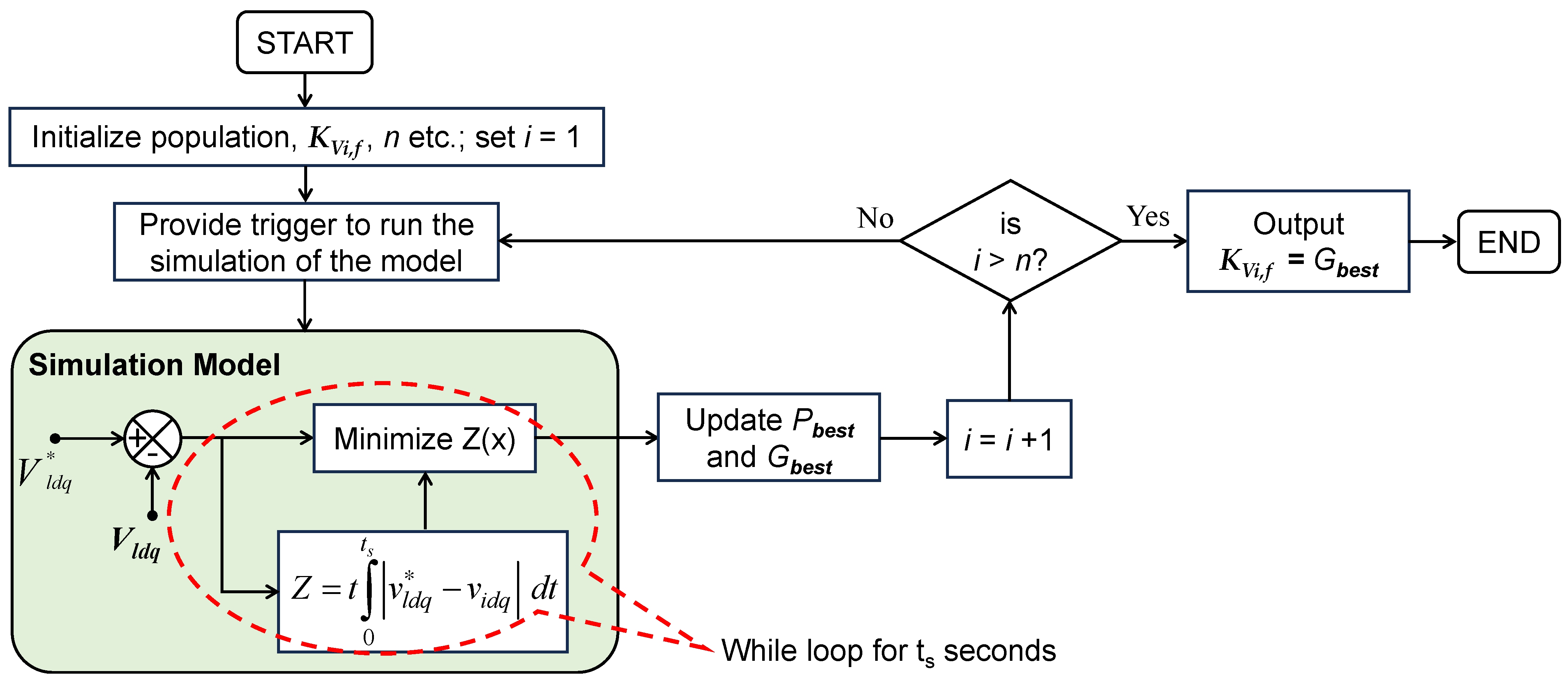
2.2. MPZC Description

With the conventional PZC method, the tuning of the forward controllers in the CCL is satisfactory. Thus, the proportional and integral coefficients of these controllers are fixed based on the conventional PZC method. However, when conventional PZC is applied to design the forward controllers of the VCL, its integral constant (KVi,f) is obtained as zero. This hampers the applicability of PZC for tuning VCL and CCL. Therefore, to obtain an optimal and reliable value for KVi,f, the PSO is used in the MPZC method. The objective of the PSO in this case is to minimize the objective function ‘Z’, which is the integral time absolute error of V l d q and V l d q as shown in (13). In view of this, the corresponding optimization problem is described as shown in (14), where Z(x) represents the fitness function with respect to the design variable ‘x’, which is KVi,f in this case. Further, the value of KVi,f is restricted between the lower bound ‘xlb’ and upper bound ‘xub’.
Z = t 0 t s | v l d q v l d q |   d t
M i n i m i z e   Z ( x ) x = K V i , f s u b j e c t   t o   x l b x x u b }
A flow chart which depicts the procedure involved in finding the optimum KVi,f using the PSO in MPZC is shown in Figure 4. In this process, to begin with, initial values are assigned for population size and the decision variable. This is followed by initializing the velocity and position of each particle in the population.
A value for the maximum number of iterations ‘n’ is assigned, and the iteration count ‘i’ is initialized to 1. With this, the process begins, and a trigger signal is provided to simulate the model. As this simulation will continue to execute in the loop for the entire simulation time of ts seconds uninterruptedly, this is referred to as a while loop in the flow chart. After ts seconds, the best fitness of any particle is assigned for Gbest. Next, the value of i is incremented by 1, and the condition, if i > n has occurred, will be checked. If the condition is not met, then it prompts the triggering of the while loop of the simulation model for one more time. The repetition of this cycle continues till the condition i > n is reached. Once the condition is satisfied, the algorithm assigns the final updated value of Gbest as the optimum value of KVi,f.

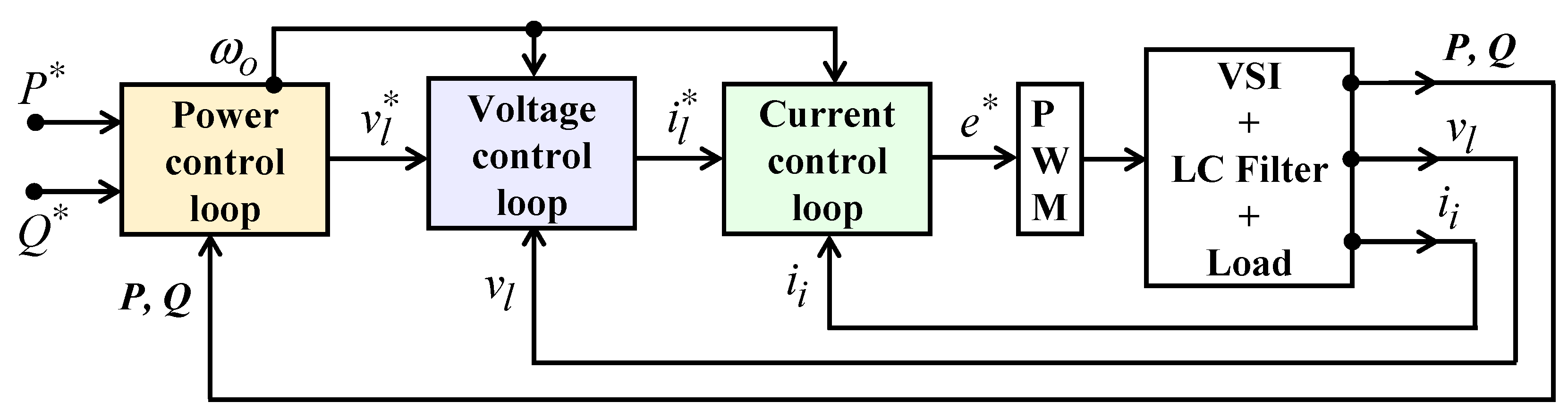
3. Proposed Methodology: Overview and Implementation

The details of the power, voltage, and current controllers for both the conventional and proposed control schemes are described in Figure 5. In this figure, the difference between the conventional and proposed methods is highlighted in the proposed methodology for a quick understanding of the proposed changes. In the proposed methodology, the performance of the MPZC-tuned forward controllers is enhanced with the performance of IMC-based multivariable controllers in the cross-coupling paths. This methodology is implemented for both the voltage and current controllers. The necessary details required for the implementation of the proposed methodology are discussed in the following subsections. In this work, an adaptive droop control that is implemented through fuzzy logic [39] is deployed for the power control loop. To avoid repetition, the details pertaining to its implementation are not furnished in this paper. So, this paper provides the modeling of the proposed CCL and VCL as follows.

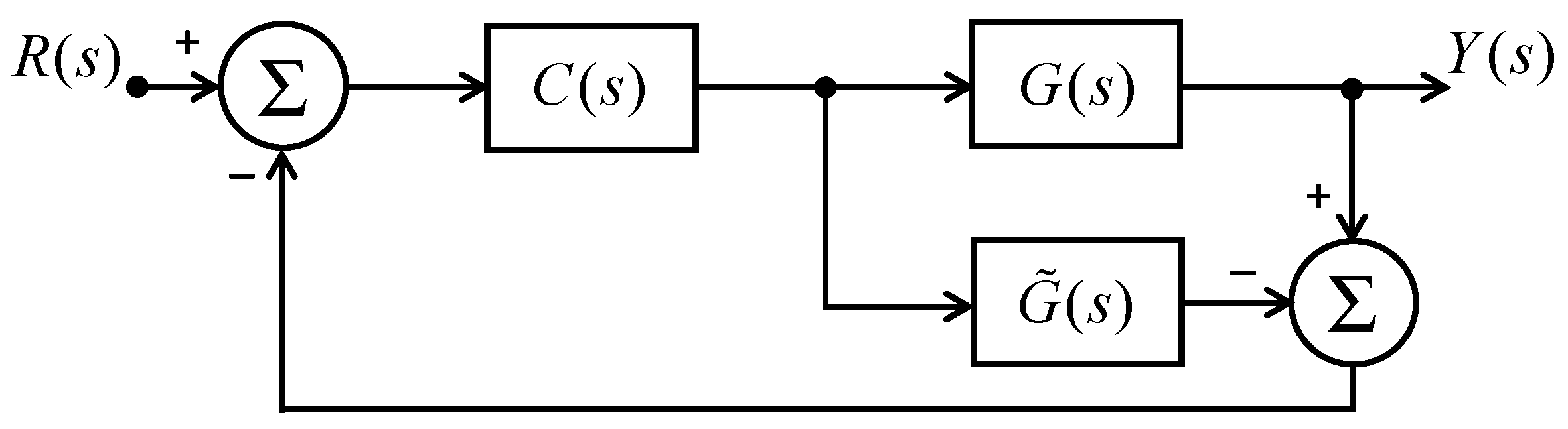
3.1. Overview of Direct Synthesis Method

Consider the model of a typical feedback control system as depicted in Figure 6. With R(s) and Y(s) as the Laplace transform of the input and output, the closed-loop transfer function is expressed as shown in (15), where G(s) is the plant transfer function that represents the process to be controlled and C(s) is the controller transfer function. In the direct synthesis method, C(s) is solved by specifying the desired closed-loop response to obtain the required controller, as shown in (16).
Y ( s ) R ( s ) = G ( s ) C ( s ) 1 + G ( s ) C ( s )
C ( s ) = 1 G ( s ) × 1 1 Y ( s ) / R ( s ) | d e s i r e d 1

3.2. IMC Model Design Based on Direct Synthesis

Here, the direct synthesis procedure of deriving the IMC-based controller for a typical feedback control system is discussed. The conventional block diagram model for the design of the IMC controller for this case is depicted in Figure 7.
G ˜ ( s ) is an exact or approximate representation of the process model G(s) to be controlled. Importantly, the IMC ensures system stability only when both G(s) and C(s) remain stable, assuming that the process model G ˜ ( s ) accurately represents the underlying process. Hence, the design of the IMC system is uncomplicated when the process model is both exact and minimum-phase. In such a case, G(s) and G ˜ ( s ) are equal and can be used for using the direct synthesis method. The plant model can be segregated into invertible and non-invertible parts, as shown in (17), where G ˜ i ( s ) is the invertible part and G ˜ n i ( s ) is the non-invertible part. In the IMC method, the primary target of the feedback controller is to follow the desired closed-loop response that is depicted in (18), where “f(s)” is the low-pass filter as shown in (19).
G ( s ) = G ˜ ( s ) = G ˜ i ( s ) G ˜ n i ( s )
Y ( s ) R ( s ) | d e s i r e d = G ˜ n i ( s ) . f ( s )
f ( s ) = 1 ( λ s + 1 ) n
To guarantee that the IMC controller is proper, the choice of “λ” and “n” in (19) is crucial. After deriving the desired closed-loop response as given in (18), the direct synthesis method shown in (16) is applied to derive the IMC controller as shown in (20).
1 G ( s ) = 1 G ˜ i ( s ) G ˜ n i ( s ) = G ˜ i 1 ( s ) G ˜ n i ( s ) 1 1 Y ( s ) / R ( s ) | d e s i r e d 1 = 1 1 G ˜ n i ( s ) f ( s ) 1 C ( s ) = G ˜ i 1 ( s ) f ( s ) 1 [ G ˜ n i ( s ) f ( s ) ] = G ˜ i 1 ( s ) 1 ( 1 / f ( s ) ) G ˜ n i ( s ) }

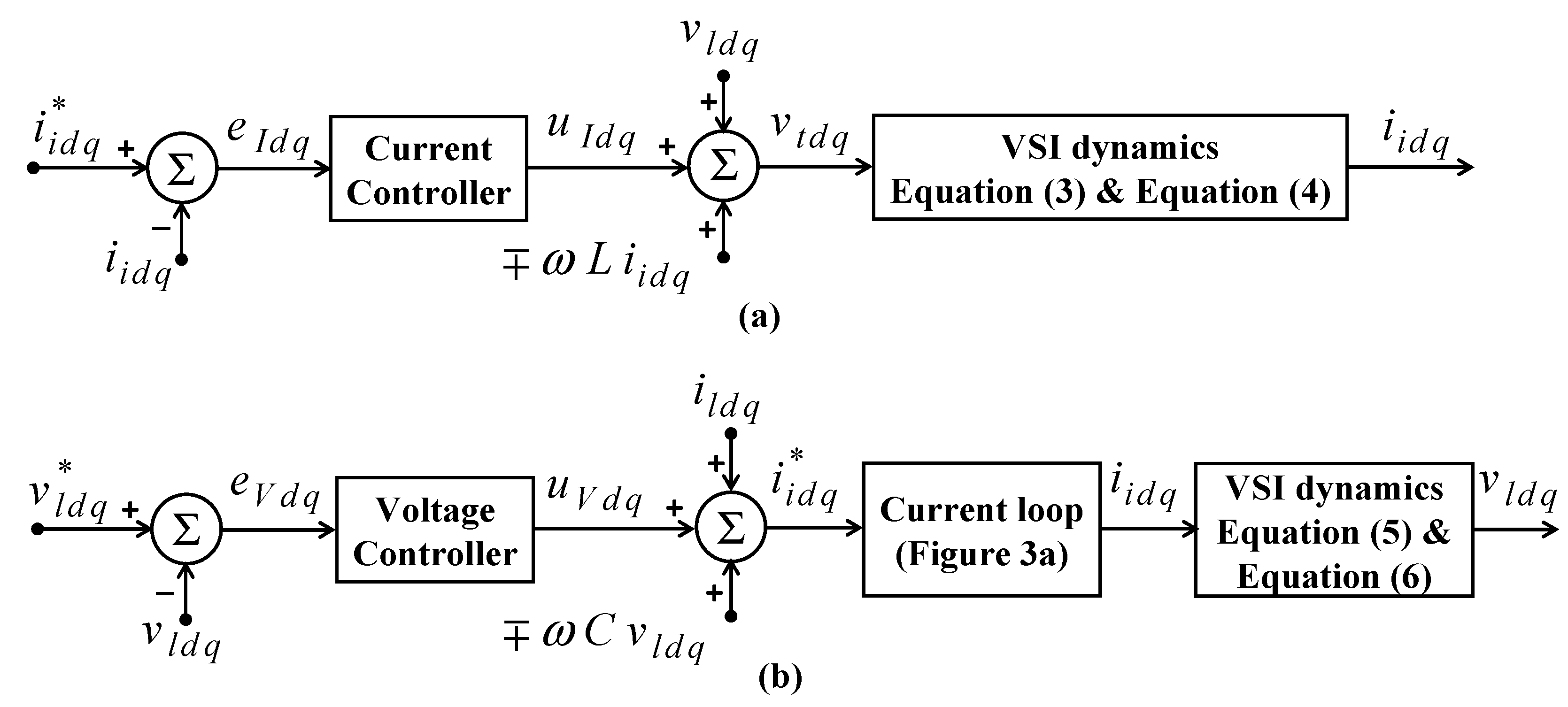
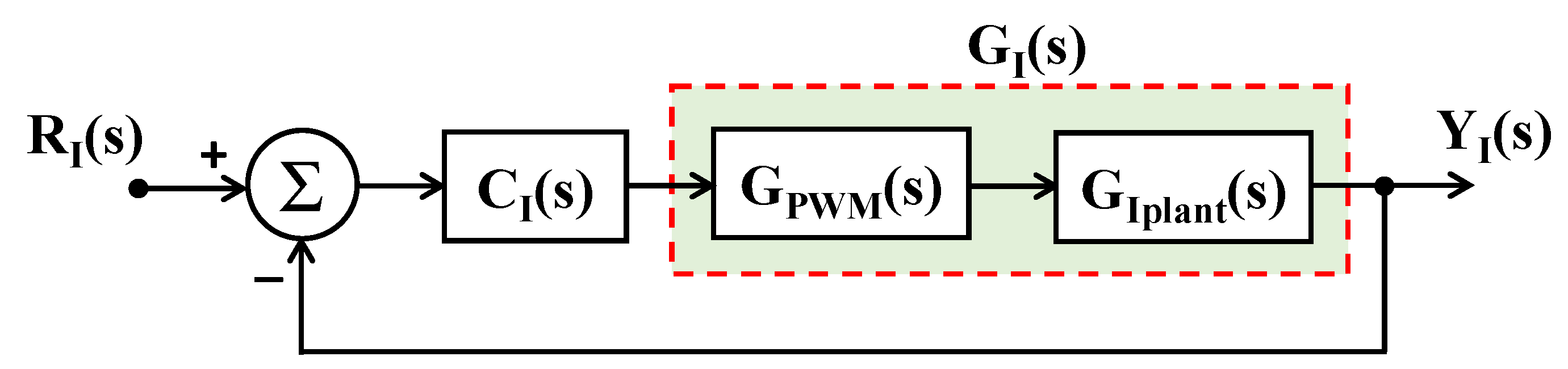
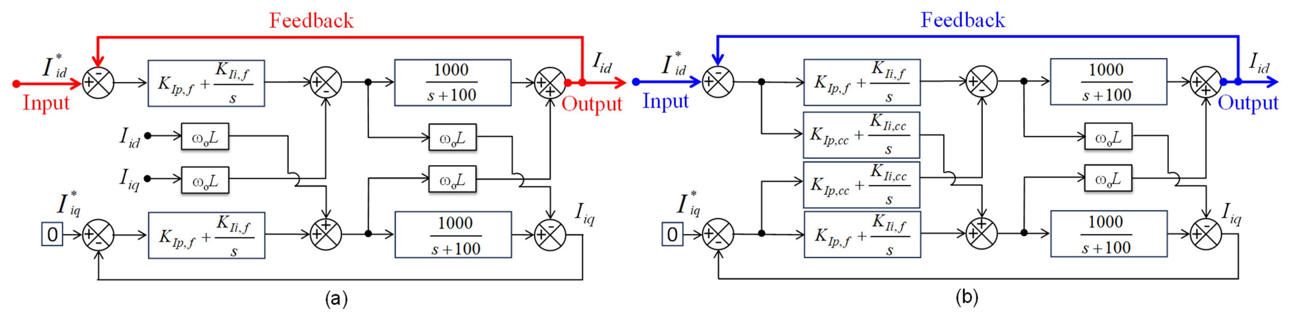
3.3. Multivariable Inner CCL Design for VSI

Here, the direct synthesis way of designing an IMC control for designing the controllers in the cross-coupling paths of the CCL is discussed. The corresponding model of the inner CCL is depicted in Figure 8. The plant transfer function that is shown in (21) is based on (7). The time delay associated with the PWM is modeled as shown in (22). The effective overall plant transfer function GI(s) in the CCL that is based on (21) and (22) is expressed as shown in (23).
V t d q ( s ) V l d q ( s ) = R ( 1 + L R ( s + j ω ) ) I i d q ( s ) G I p l a n t ( s ) = I i d q ( s ) V t d q ( s ) V l d q ( s ) = K 1 + ( s + j ω ) T I } w h e r e   K = 1 / R   a n d   T I = L / R
G P W M ( s ) = 1 1 + ( s + j ω ) T P W M
G I ( s ) = K [ 1 + ( s + j ω ) T I ] [ 1 + ( s + j ω ) T P W M ]
As described in (17), the plant model can be segregated into invertible part GI(s) and non-invertible part G ˜ I n i ( s ) as shown in (24). GI(s) is the minimum phase and has no zeros in the right half of the s-plane. In such a case, G ˜ I n i ( s ) = 1 . Considering n = 1 in (19), f(s) in this case is expressed as shown in (25). In such a case, the desired closed-loop response can be expressed as shown in (26). Thus, the effective controller is obtained in (27).
G I ( s ) = G ˜ I i ( s ) G ˜ I n i ( s )
f ( s ) = 1 λ I s + 1
Y I ( s ) R I ( s ) | d e s i r e d = 1 λ I s + 1
C I ( s ) = G ˜ I i 1 ( s ) 1 λ I s = [ 1 + ( s + j ω ) T I ] [ 1 + ( s + j ω ) T P W M ] K λ I s = s 2 T I T P W M + s ( T P W M + T I ) T I T P W M ω 2 + 1 K λ I s C I r e a l ( s ) + j ω [ ( T P W M + T I ) + 2 T I T P W M s ] K λ I s C I i m a g ( s ) }
Segregating the real and imaginary parts as C I ( s ) = C I r e a l ( s ) + j C I i m a g ( s ) , the real part of (27) defines the controller in the forward path and the imaginary part will define the controller in the cross-coupling paths. As the controllers in the forward paths are designed through MPZC, we neglect the real part of CI(s). Therefore, we consider only the imaginary part that refers to the controllers in the cross-coupling paths, which is expressed as shown in (28).
C I i m a g ( s ) = C I , c c ( s ) = ω [ ( T P W M + T I ) + 2 T I T P W M s ] K λ I s
By equating (28) with the parallel structure of the PID controller that is expressed as C I , c c ( s ) = K I p , c c + K I i , c c s + s K I d , c c , the corresponding proportional, integral, and derivative coefficients are obtained as shown in (29).
K I p , c c = 2 ω T I T P W M K λ I K I i , c c = ω ( T P W M + T I ) K λ I K I d , c c = 0 }

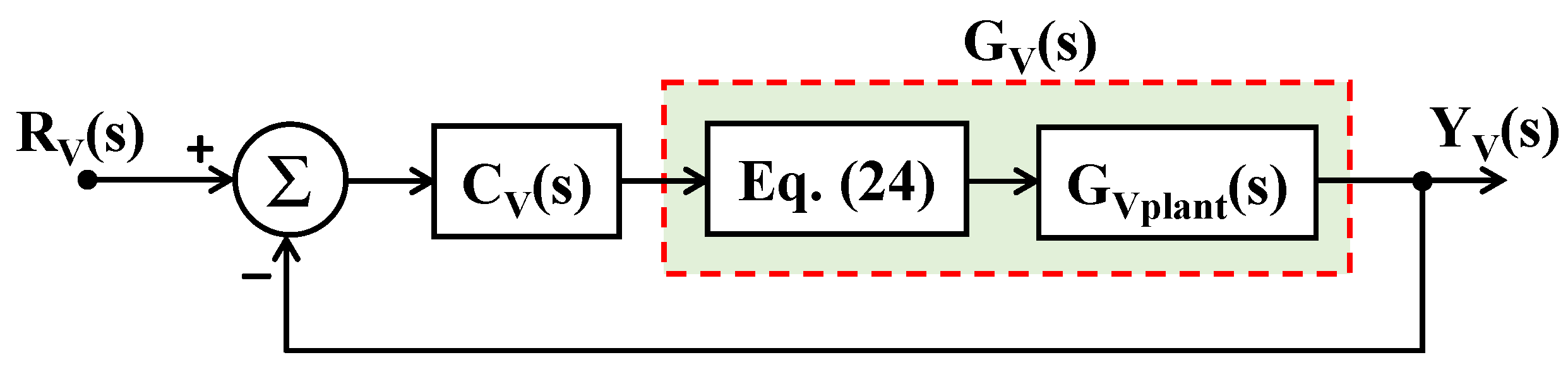
3.4. Multivariable Outer VCL Design for VSI

Here, the direct synthesis way of designing an IMC control for designing the controllers in the cross-coupling paths of the VCL is discussed. The corresponding model of the VCL is depicted in Figure 9. The plant transfer function that is shown in (30) is based on (8). As the CCL is inside the VCL, the desired response of the CCL, as shown in (26), is also included. Thus, the overall plant transfer function GV(s) in the VCL is obtained as (31).
G V p l a n t ( s ) = 1 C ( s + j ω )
G V ( s ) = Y I ( s ) R I ( s ) | d e s i r e d G V p l a n t ( s ) = 1 λ I s + 1 G V p l a n t ( s ) = 1 C ( s + j ω ) ( λ I s + 1 )
As described in (17), the plant model can be segregated into an invertible part G ˜ V i ( s ) and a non-invertible part G ˜ V n i ( s ) as shown in (32). Considering n = 1 in (19), f(s) in this case is expressed as (33).
G V ( s ) = G ˜ V i ( s ) G ˜ V n i ( s )
f ( s ) = 1 λ V s + 1
In such a case, the desired closed-loop response can be expressed as shown in (34). Thus, the effective controller is obtained as shown in (35).
Y V ( s ) R V ( s ) | d e s i r e d = 1 λ V s + 1
C V ( s ) = G ˜ V i 1 ( s ) 1 λ V s = C ( s + j ω ) ( λ I s + 1 ) λ V s
Segregating the real and imaginary parts as C V ( s ) = C V r e a l ( s ) + j C V i m a g ( s ) , the real part of (35) defines the controller in the forward path and the imaginary part will define the controller in the cross-coupling paths. As the controllers in the forward paths are designed through MPZC, we neglect the real part of CV(s). Therefore, we consider only the imaginary part that refers to the controllers in the cross-coupling paths, which is expressed as shown in (36).
C V i m a g ( s ) = C V , c c ( s ) = ω C λ I λ V + ω C λ V s
By equating (36) with the parallel structure of the PID controller that is expressed as C V , c c ( s ) = K V p , c c + ( K V i , c c / s ) + s K V d , c c , the corresponding proportional, integral, and derivative coefficients are obtained as shown in (37).
K V p , c c = ω C λ I λ V K V i , c c = ω C λ V K V d , c c = 0 }

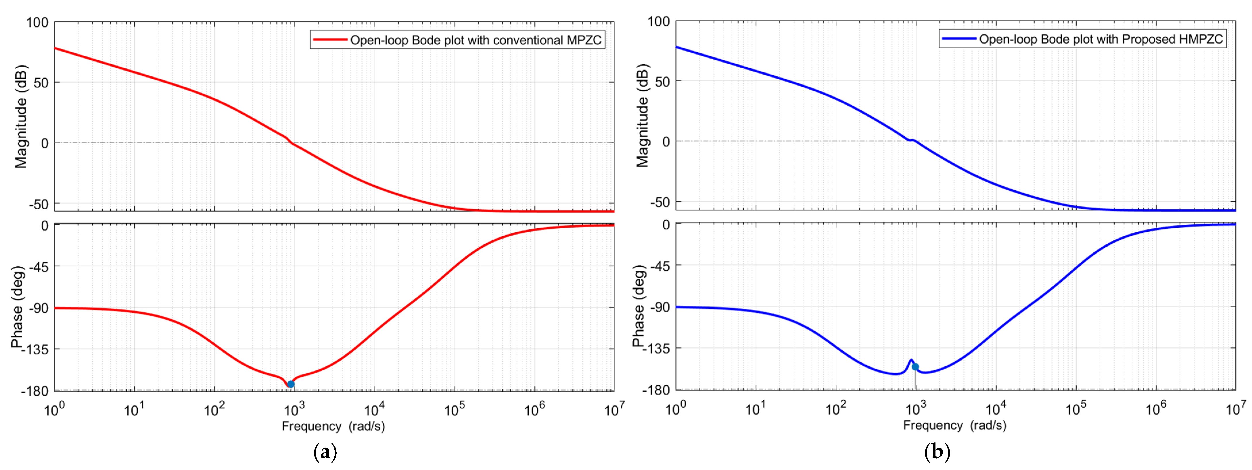
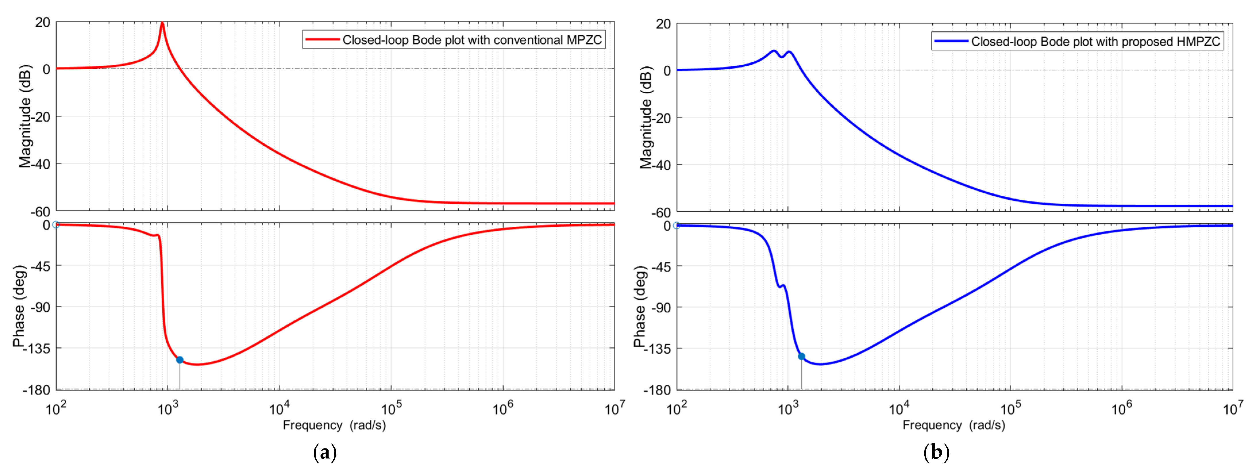
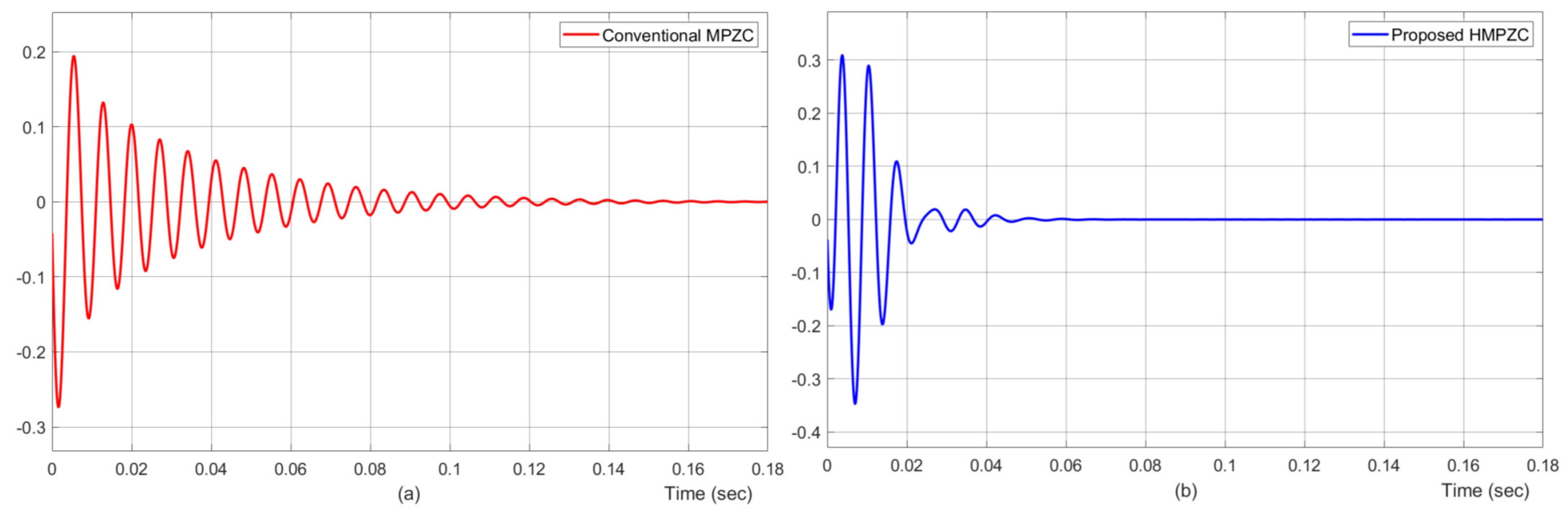
3.5. Rationale of Proposed HMPZC

As the CCL is the innermost control loop, its dynamics primarily affect the transient response of the overall system. In view of this, here the performance of the conventional MPZC and proposed HMPZC methods are compared based on the response of the CCL with these methods. As the analysis with the VCL will follow similar steps, in order to avoid repetition, the discussion will be limited to the CCL only.
The complete implementation of the CCL model shown in Figure 8 is represented in Figure 10, where the CCL design for conventional MPZC is shown in Figure 10a while the CCL for the proposed HMPZC is shown in Figure 10b. Both the models have two inputs I i d , I i q and two outputs I i d , I i q . Here, the procedure is discussed to study the effect of I i d on I i d or on I i q . For this purpose, the other input I i q is made zero, and thereafter the closed-loop response is obtained. Whereas, for an open-loop response, the feedback path is removed and the response is recorded. After substituting the controller parameter values that are available in Section 4, the overall open-loop and closed-loop transfer functions of the conventional MPZC and proposed HMPZC are expressed as shown in (38)–(41). The reader can use either the block diagram model or transfer functions to reproduce the obtained Bode plots and step responses.
I i d ( s ) I i d ( s ) | O p e n L o o p M P Z C = 0.001435 s 4 + 140.6 s 3 + 9.022 × 10 5 s 2 + 2.876 × 10 8 s + 6.469 × 10 11 s 4 + 321.2 s 3 + 7.303 × 10 5 s 2 + 8.079 × 10 7 s
I i d ( s ) I i d ( s ) | C l o s e d L o o p M P Z C = 0.001433 s 4 + 140.4 s 3 + 9.009 × 10 5 s 2 + 2.872 × 10 8 s + 6.46 × 10 11 s 4 + 461.1 s 3 + 1.63 × 10 6 s 2 + 3.679 × 10 8 s + 6.46 × 10 11
I i d ( s ) I i d ( s ) | O p e n L o o p H M P Z C = 0.001322 s 6 + 139.1 s 5 + 8.933 × 10 5 s 4 + 2.848 × 10 8 s 3 + 6.406 × 10 11 s 2 + 0.0001826 s + 4.219 × 10 20 s 6 + 320.1 s 5 + 8.219 × 10 5 s 4 + 7.999 × 10 7 s 3 2.349 × 10 10 s 2
I i d ( s ) I i d ( s ) | C l o s e d L o o p H M P Z C = 0.0013 s 6 + 138.9 s 5 + 892120 s 4 + 2.844 × 10 8 s 3 + 6.398 × 10 11 s 2 + 0.0001824 s + 4.213 × 10 20 s 6 + 458.6 s 5 + 1.713 × 10 6 s 4 + 3.643 × 10 8 s 3 + 6.398 × 10 11 s 2 + 0.0001824 s + 4.213 × 10 20
The open-loop and closed-loop Bode plots obtained for the conventional and proposed methods are given in Figure 11 and Figure 12, respectively. From the open-loop Bode plots in Figure 11a,b, it is seen that the conventional method shows a gain crossover frequency of 900 rad/s, while the proposed method shows 1000 rad/s. From the closed-loop Bode plots in Figure 12a,b, it is seen that both methods show a bandwidth of ≈2000 rad/s. However, the peak gain of HMPZC is lesser than that of MPZC, which leads to better damping with HMPZC. The effect of this peak gain on the transient response of the conventional and proposed methods is seen in the step responses.
The performance of the conventional MPZC and proposed HMPZC methods are compared based on their individual step responses. For this purpose, step inputs are provided to the d-axis, and the corresponding outputs are recorded in the d- and q-axes. Figure 13a,b show the output response of the MPZC and HMPZC methods in the d-axis (forward path). With HMPZC, the output settled within 0.03 s, whereas with MPZC, the output took around 0.14 s to settle.
From these figures, it is to be noted that even though the controller parameters in the forward paths of both HMPZC and MPZC are the same, the responses are different. The possible cause for this can be attributed to the differences in the cross-coupling paths. The following discussion confirms the aforesaid hypothesis. For the input I i d , its effect on I i q (the cross-coupling path) was studied based on the step responses obtained, as shown in Figure 14. It is noticed from these results that by 0.02 s, the impact of the cross-path is almost nullified in the proposed method (Figure 14b). Whereas, oscillations with a substantial amplitude continued to exist with the conventional method up to 0.1 s (Figure 14a). This confirms that the superior performance of the proposed method over the conventional method is due to reduced coupling between the d- and q-axes loops with the proposed HMPZC method.

4. Simulation Results and Discussion

Here, the response of the proposed hybrid MPZC (HMPZC) is analyzed and evaluated under three different test cases, T1, T2, and T3. In all the test cases, load 1 receives power during the entire time, while load 2 receives power from 80–90 s. The reactive load component of load 2 is gradually increased from T1 to T3. During the design of these test cases, the selection of load 2 is selected carefully to create the conditions of extremely poor power factor loadings during 80–90 s. A summary of the various test cases that are used for the evaluation of this work is shown in Table 1. The frequency, active power, voltage, and voltage total harmonic distortion (THD) results under various test cases are compared to analyze the performance of the HMPZC and MPZC schemes.
The maximum P-ω and Q-v droop coefficient values that are used in the development of an adaptive fuzzy logic-based droop control for the APL and RPL are provided in Table 2. Further, from the system parameters mentioned in Section 2, and depending on the method described in Section 3, various gain coefficients of the voltage and current controllers in the forward and cross-coupling paths are provided in Table 2. In the same table, “NA” refers to not applicable.
The performance of the proposed method can be analyzed with reference to similar works [4,18,19,39], and [40]. Among these, refs. [4,40] are the works of other authors. As the present work is an extension of [19], this study will be credible if the performance of the proposed method is analyzed with reference to [4,19], and [40]. These methods are tested under a common test case, T1. The maximum value of frequency due to the load switch being on is 50.4 Hz with [4], 58.6 Hz with [40], and ≈50 Hz with [19] and the proposed HMPZC. The minimum frequency due to the load switch being off is 49.6 Hz with [4], 40 Hz with [40], and ≈50 Hz with [19] and the proposed HMPZC. Thus, with respect to frequency, stable performance is achieved with [19] and the proposed method. However, unacceptable deviations in frequency are noticed in [4,40]. Further, refs. [4,40] have failed to maintain power stability, while [19] and the proposed method have successfully maintained stability in delivering the required power during load switching. Similarly, voltage stability is lost with [4,40], whereas in the case with [19] and the proposed method, the voltage stability is maintained with a THD less than 5%. Thus, the performance of the proposed HMPZC method can be analyzed with the MPZC method of [19] only under T2 and T3. It is to be noted that the results and discussions, as provided in Section 4.1, Section 4.2 and Section 4.3, describe the performance of the conventional MPZC and HMPZC methods.

4.1. Results and Discussion Corresponding to Test Case T1

Here, the performance of the HPMZC and MPZC schemes under test case T1 are compared and discussed. The frequency results (Figure 15a,b) identify that both schemes are stable. The deviation in the frequency under load 2 switch ON (shown by Figure 15c) is 0 Hz with MPZC and HMPZC. In the case of load 2 switch OFF (shown by Figure 15d), it is identified that the deviation in the frequency is 0.015 Hz and 0.01 Hz with MPZC and HMPZC, respectively. Thus, the frequency is the stable response of both schemes, but the transient response of HMPZC is a little better than MPZC.
As the nature of load 2 is reactive, its effect on active power results as shown in Figure 16 is used to identify the dq-coupling aspect. Corresponding to the load switch ON at t = 80 s, it is seen from Figure 16a that the overshoot seen at 80 s with the proposed scheme delivers an extra burden of 1308 W. However, as seen in Figure 16b, the conventional scheme delivers an extra burden of 1529 W, which is higher than that of the proposed scheme. Further, due to load switch OFF at t = 90 s, MPZC has caused an extra burden of 851 W, while HMPZC has caused 613 W. Thus, under load switch ON and switch OFF, the proposed scheme provides a better transient response by reducing the coupling.
The voltage results of the proposed and conventional schemes are provided in Figure 17a and Figure 17b, respectively. The zoomed-in results seen in Figure 17c,d identify the similar voltage responses of both schemes. This is further confirmed by the THD plots depicted in Figure 18. The THD result of HMPZC is 3.08% (Figure 18a), which is slightly less than the conventional scheme’s 3.49% (Figure 18b). However, this cannot be claimed as an improvement, as both the values fall below the permissible 5%.

4.2. Results and Discussion Corresponding to Test Case T2

Here, the performance of the HPMZC and MPZC schemes under test case T2 are compared and discussed. The frequency results (Figure 19a,b) identify that both schemes are stable. The deviation in the frequency under load 2 switch ON (shown by Figure 19c) is 0 Hz with MPZC and HMPZC. In the case of load 2 switch OFF (shown by Figure 19d), it is identified that the deviation in the frequency is 0.02 Hz with both MPZC and HMPZC. Thus, the frequency is the stable response of both schemes, but the transient response of both HMPZC and MPZC is the same. The effect of load 2 on the active power results (Figure 20) confirms that the overshoot seen at 80 s with the proposed scheme (Figure 20a) is lesser than the conventional scheme (Figure 20b). Corresponding to the load switch ON at t = 80 s, it is seen from Figure 20a that the overshoot seen at 80 s with the proposed scheme delivers an extra burden of 1914 W. However, as seen in Figure 20b, the conventional scheme delivers an extra burden of 2307 W, which is higher than that of the proposed scheme. Further, due to the load switch OFF at t = 90 s, MPZC has caused an extra burden of 1114 W, while HMPZC has caused 928 W. This confirms that the proposed scheme has reduced the dq coupling comparatively.
The voltage results of HMPZC are provided in Figure 21a and those of MPZC are provided in Figure 21b. The zoomed-in voltage results (Figure 21c,d), confirm that the voltage response of HMPZC is smoother than that of the MPZC scheme. Further, a distortion of voltage is also identified with conventional MPZC at the instant of load removal (at 90 s), as indicated with an arrow mark in Figure 21d. This is further confirmed by the THD plots shown in Figure 22. The THD of the proposed and conventional schemes are noted as 3.33% (Figure 22a) and 5.62% (Figure 22b). Thus, the frequency and THD results confirm that the proposed HMPZC exhibits a better transient response than the conventional MPZC.

4.3. Results and Discussion Corresponding to Test Case T3

Here, the performance of the HPMZC and MPZC schemes under test case T3 are compared and discussed. The frequency results of the HMPZC and MPZC schemes are depicted in Figure 23a and Figure 23b, respectively. From the frequency results shown in Figure 23b, it is noticed that after load removal at 90 s, the conventional scheme produced a maximum deviation of 0.4 Hz, which is greater than the permissible limit of 0.05 Hz, and it has failed to maintain stability in frequency. Whereas, the proposed scheme (Figure 23a), with a deviation of 0.017 Hz, has successfully maintained a stable frequency. The effect of load 2 on the active power results that are shown in Figure 24 confirms that the overshoot of 4751 W seen at 80 s with the proposed scheme (Figure 24a) is less than that of the conventional scheme (Figure 24b), whose value is 6083 W. This confirms that the proposed scheme has reduced the dq coupling. Moreover, after 90 s, it is observed from Figure 24b that the conventional scheme has failed to maintain stability in delivering the required power to the loads. The voltage results of the HMPZC and MPZC schemes are depicted in Figure 25a and Figure 25b, respectively.
From the zoomed-in aspect of the voltage results, the voltage response of the conventional scheme (Figure 25d) is completely distorted, while that of the proposed scheme as seen in Figure 25c is satisfactory. This voltage response is further confirmed by the THD plots provided in Figure 26. From Figure 26, the THD result of the proposed scheme is 3.39% (Figure 26a), while that of the conventional scheme is 20.20% (Figure 26b). Thus, the voltage profile of HPMZC is satisfactory in its transient response and stability.

4.4. Summary of Discussions

A cumulative comparison of the frequency, active power, voltage, and voltage total harmonic distortion (THD) results under various test cases is presented in Table 3.
From this table, the following aspects are analyzed: namely, power delivery capability, transient response, and coupling between dq loops. In this table, T80 and T90 refer to instances of switch ON and switch OFF of load 2, respectively.
  • The highlighted values in the table specify an intolerable deviation regarding their characteristics.
  • From the frequency characteristics, a small deviation in overshoot or undershoot is the desired criterion to verify an improvement in transient response.
  • From the power characteristics, “stable” in the stability criteria is the desired outcome to verify power delivery capability.
  • From the power characteristics, a smaller value in extra burden is used to verify a reduction in dq coupling.
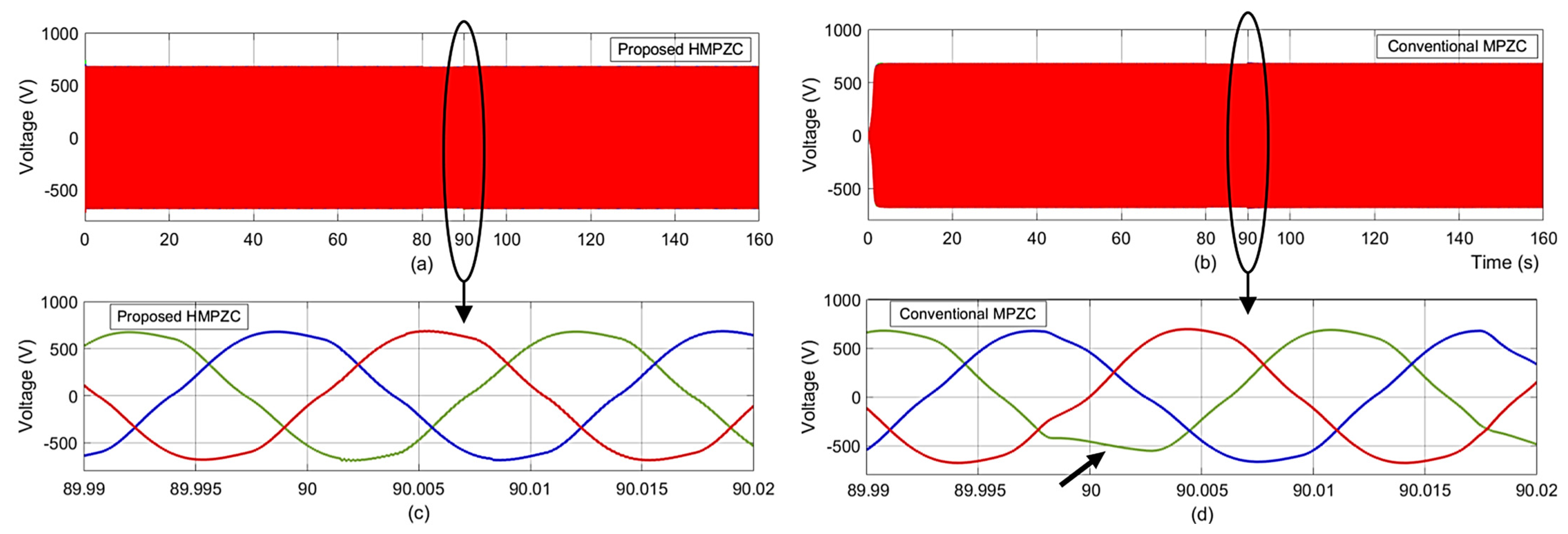
  • From the voltage characteristics, the THD value is used to verify transient response improvement. “NC” in the same characteristics indicates not considered.

5. Conclusions

In this paper, the HMPZC method, which combines multivariable control with the MPZC method, is proposed. For this purpose, the proposed IMC-based multivariable PI controllers are realized using the direct synthesis method. This helps to improve the vector control of VSIs by reducing the coupling between the d- and q-axes loops of current/voltage in the VSI’s multiloop control structure, thereby enhancing the transient response and power delivery capability. The influence of dq coupling is inferred from the extra burden aspect of the active power results, and the quality of the transient response is inferred from the frequency and voltage characteristics. Similarly, the power loop’s power delivery capacity is inferred from the system stability aspect of the power characteristics. Based on these three key performance indices, the performance of the proposed HMPZC method and conventional MPZC method under various test cases is summarized as follows.
Under test case T1:
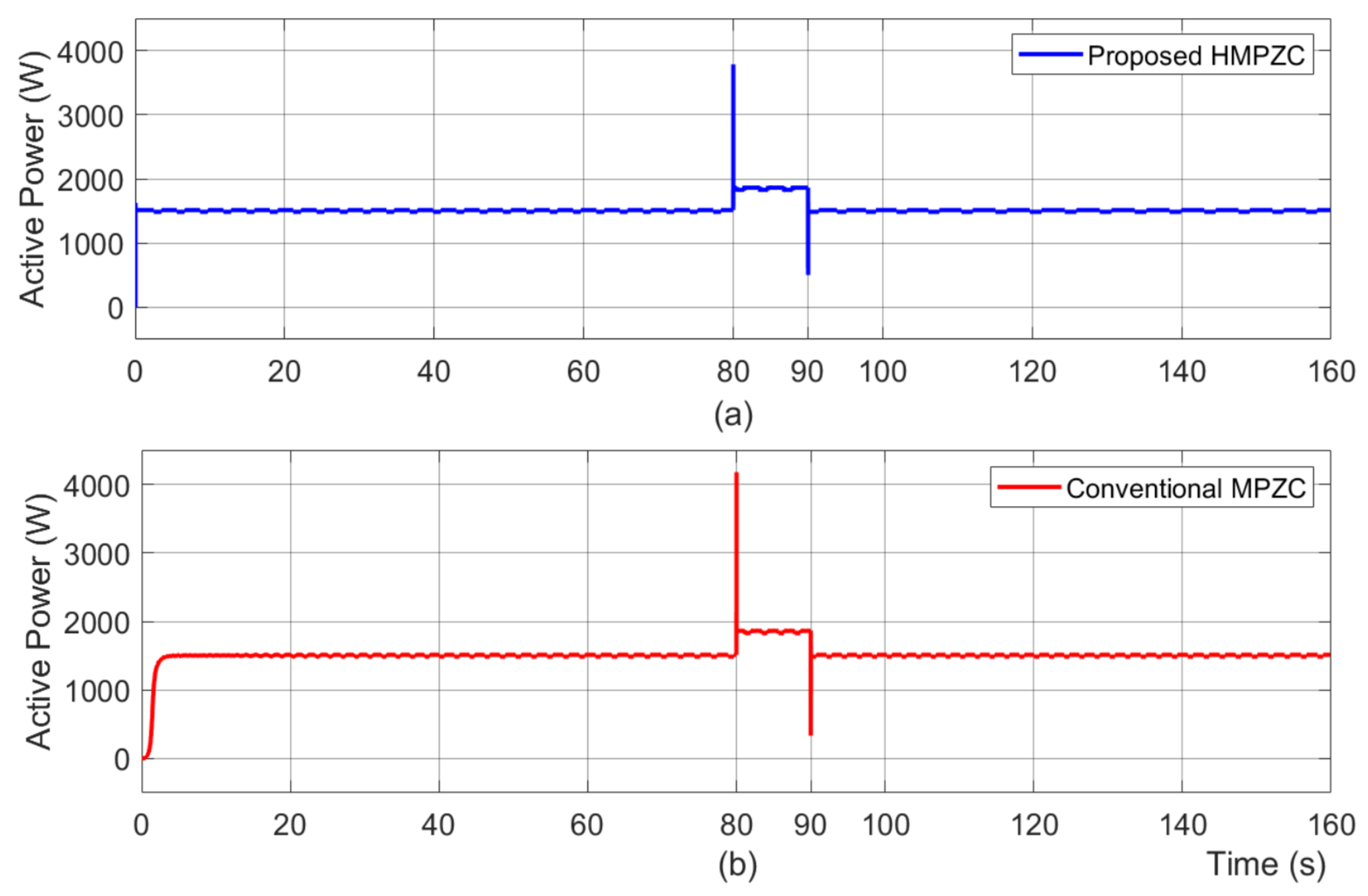
  • The overshoot seen in the active power is 1308 W with the HMPZC method and 1529 W with the conventional MPZC method. This confirms that a reduced coupling is achieved with the proposed HMPZC method.
  • An improvement in transient response cannot be inferred, because the deviation in frequency is the same, and the voltage THD values are less than 5% with both methods.
  • As both methods ensured system stability, an improvement in power delivery capability cannot be inferred.
Under test case T2:
  • The overshoot seen in the active power is 1914 W with the HMPZC method and 2307 W with the conventional MPZC method. This confirms that a reduced coupling is achieved with the proposed HMPZC method.
  • The voltage THD with the HMPZC and MPZC methods is 3.33% and 5.62%. Unlike T1, the THD results confirm the ability of the proposed HMPZC method to improve the transient response.
  • Similar to T1 in this test case also, an improvement in power delivery capability cannot be inferred, as both methods maintained the stability of the system.
Under test case T3:
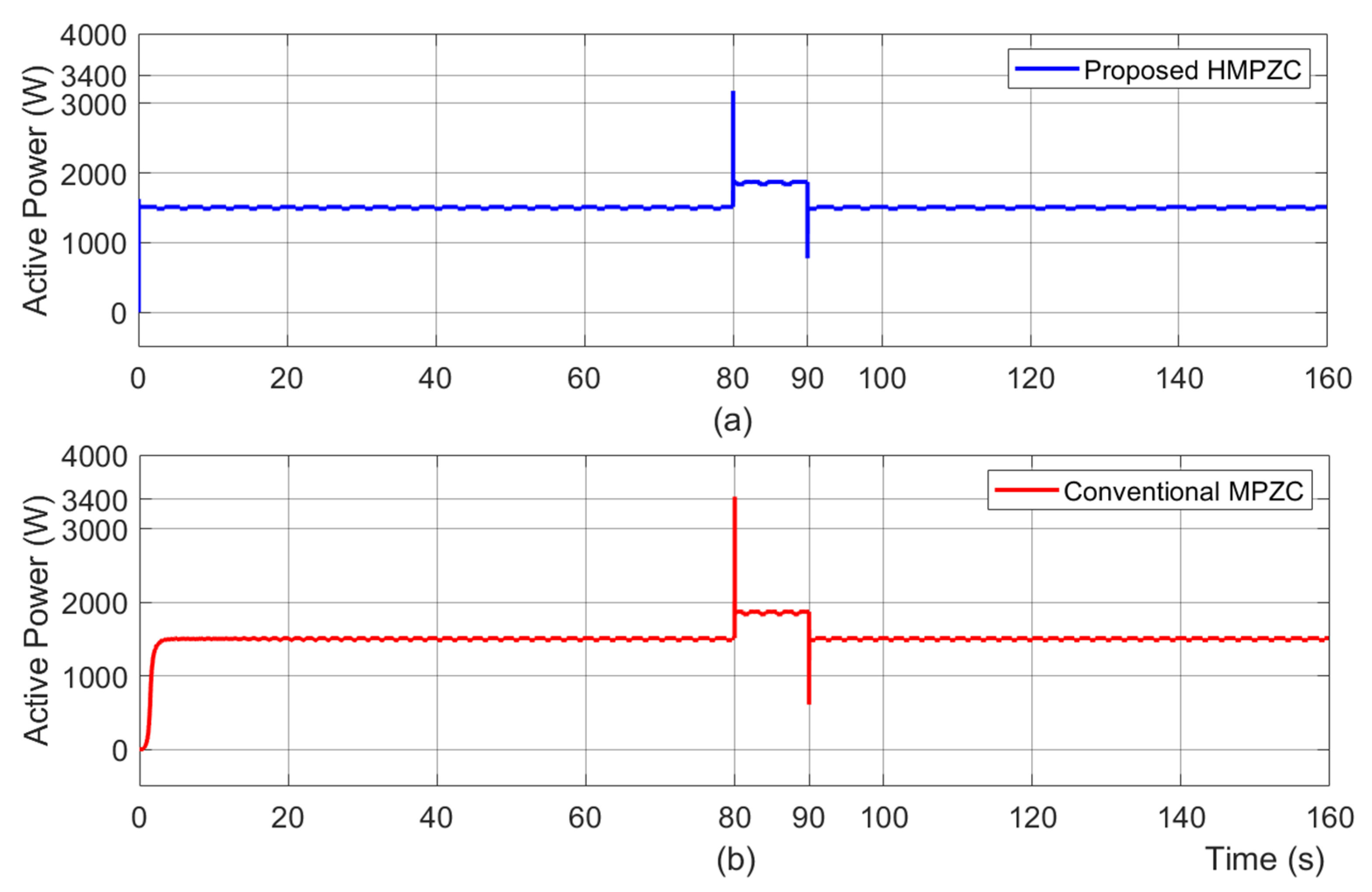
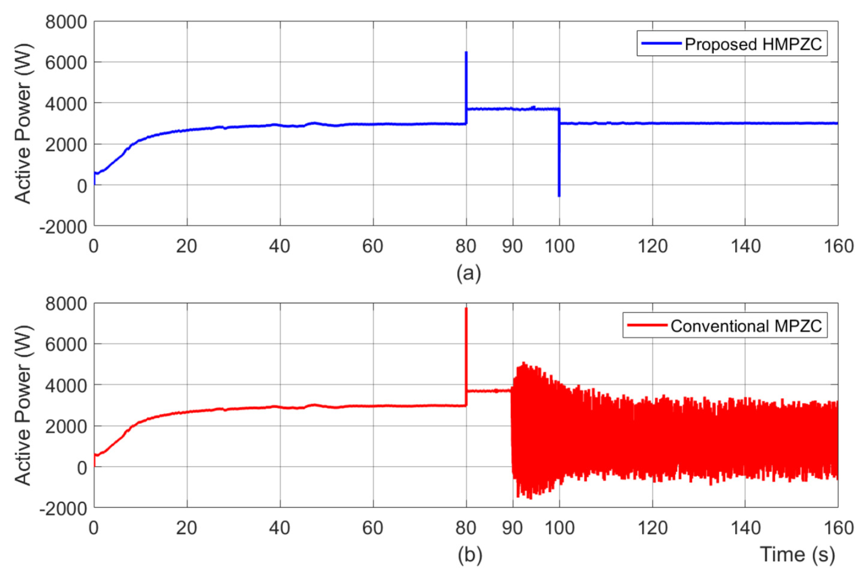
  • The overshoot seen in the active power is 4751 W with the HMPZC method and 6083 W with the conventional MPZC method. This confirms that a reduced coupling is achieved with the proposed HMPZC method.
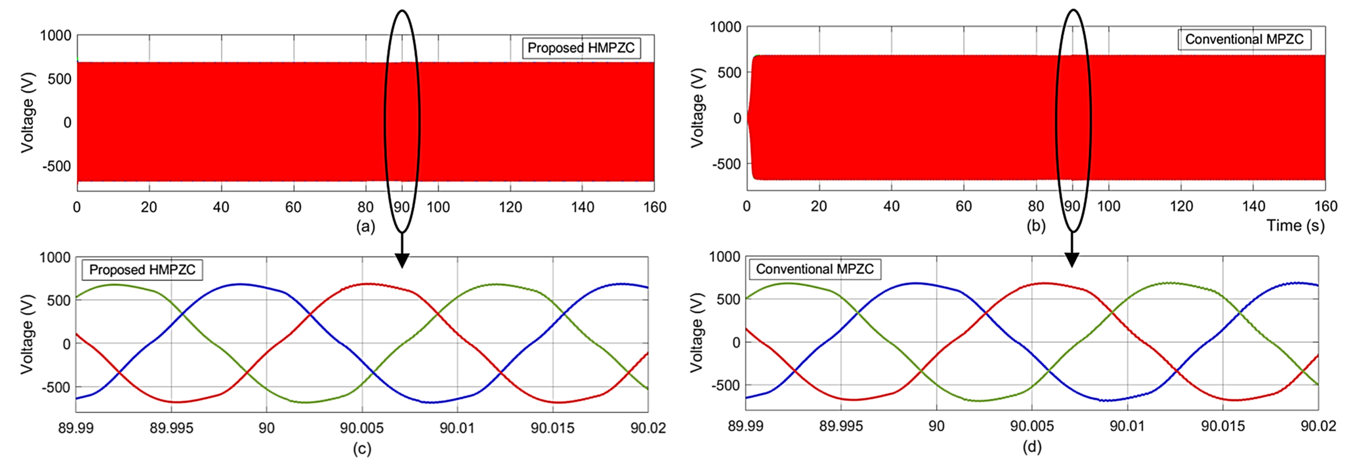
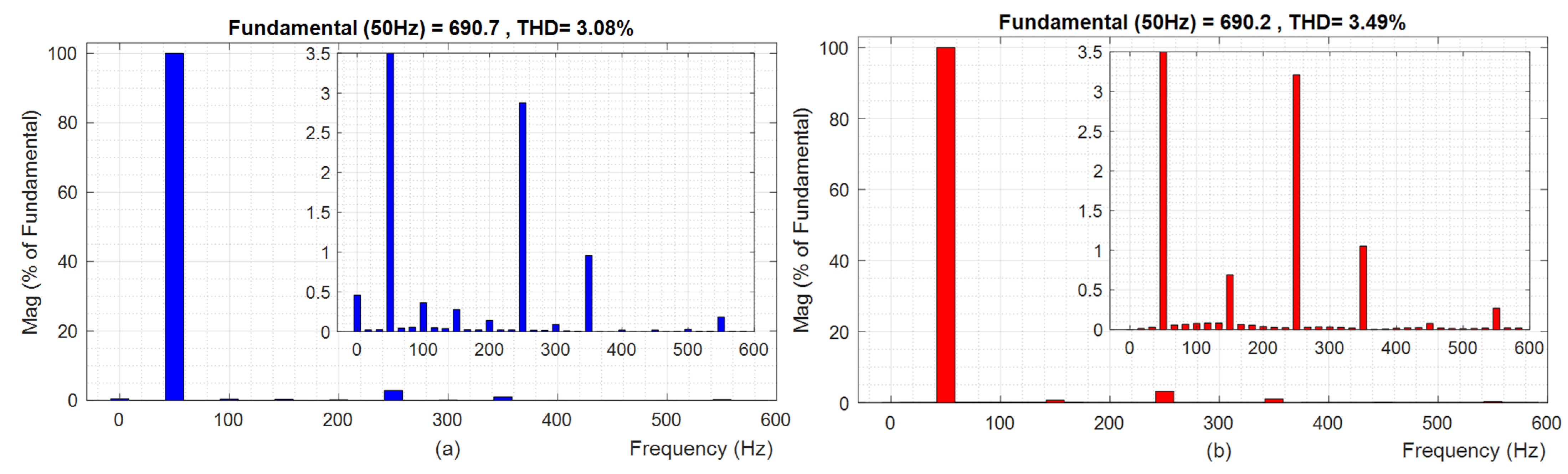
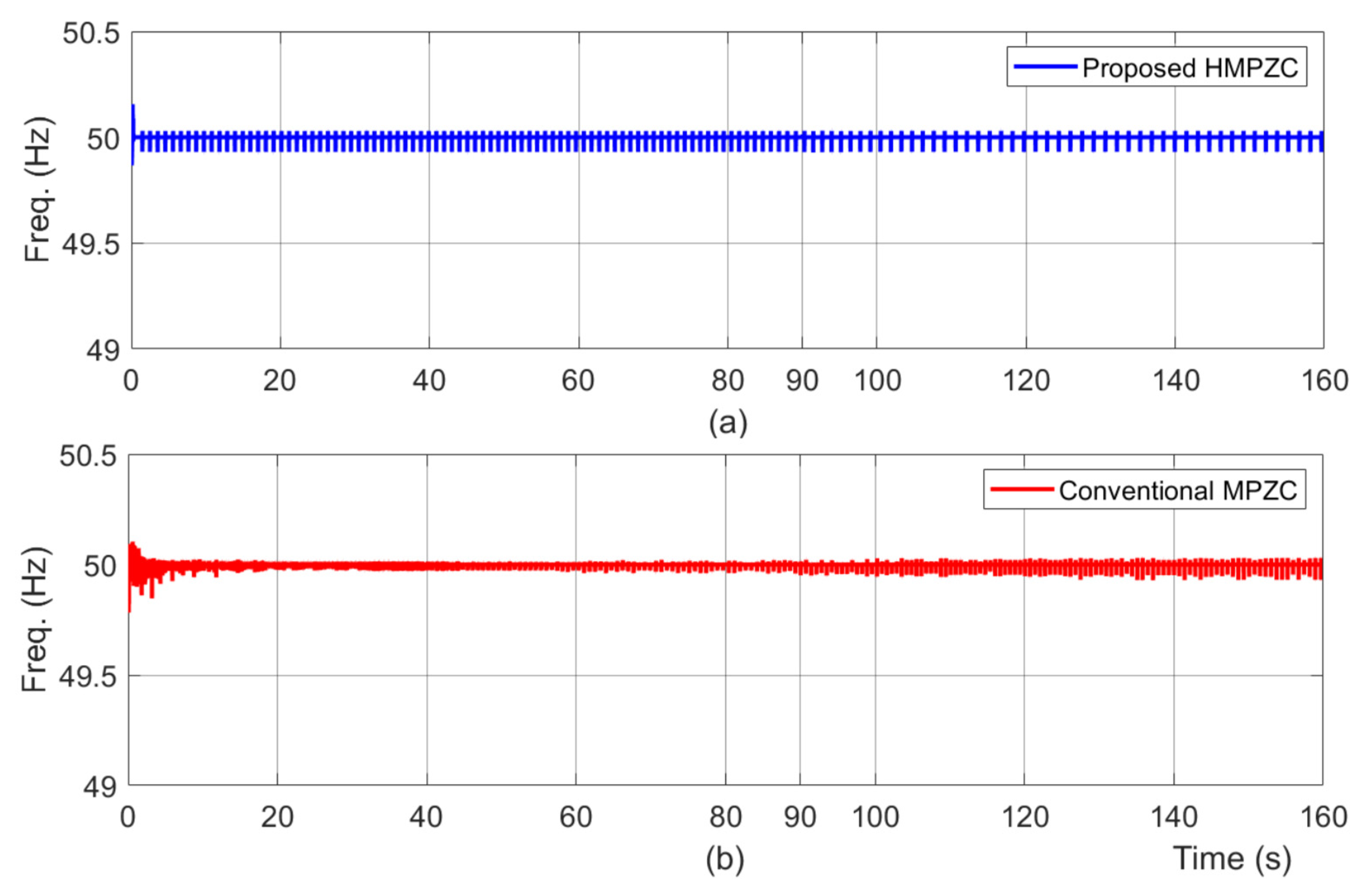
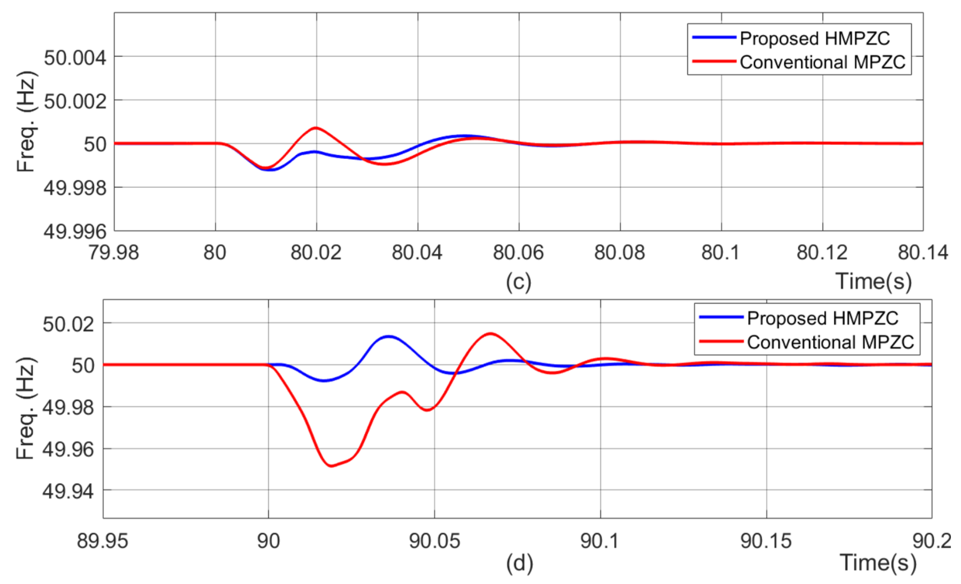
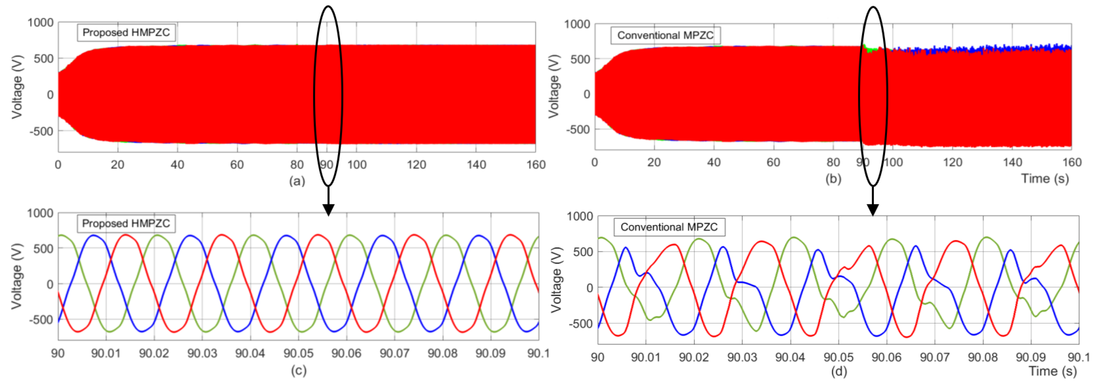
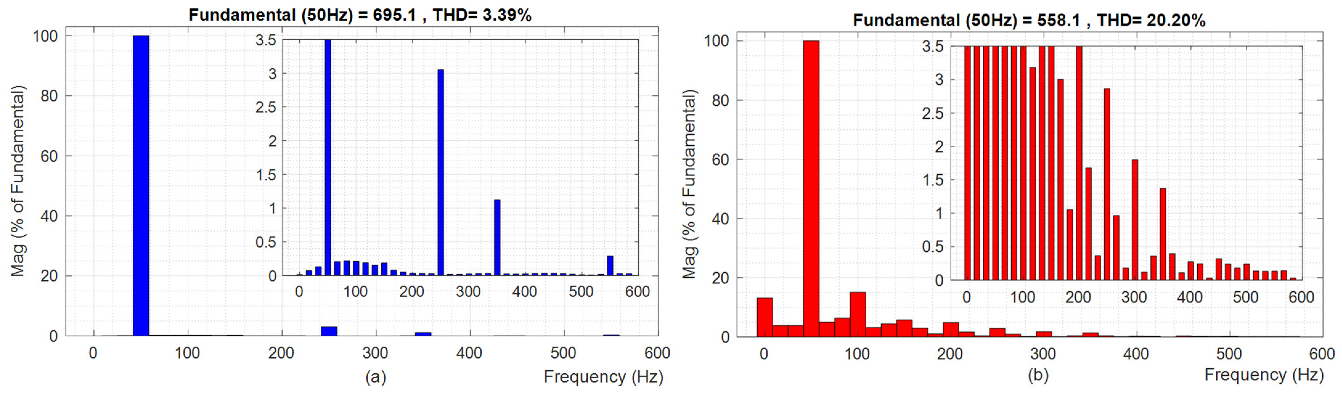
  • The maximum deviations during overshoot and undershoot with the HMZC method are 0.025 Hz and 0.017 Hz, respectively. On the other hand, the maximum deviation during overshoot and undershoot with the MPZC method is 0.4 Hz. The voltage THD with the HMPZC and MPZC methods are 3.39% and 20.2%, respectively. Thus, based on the frequency and voltage results, the ability of the proposed HMPZC method to improve the transient response is confirmed.
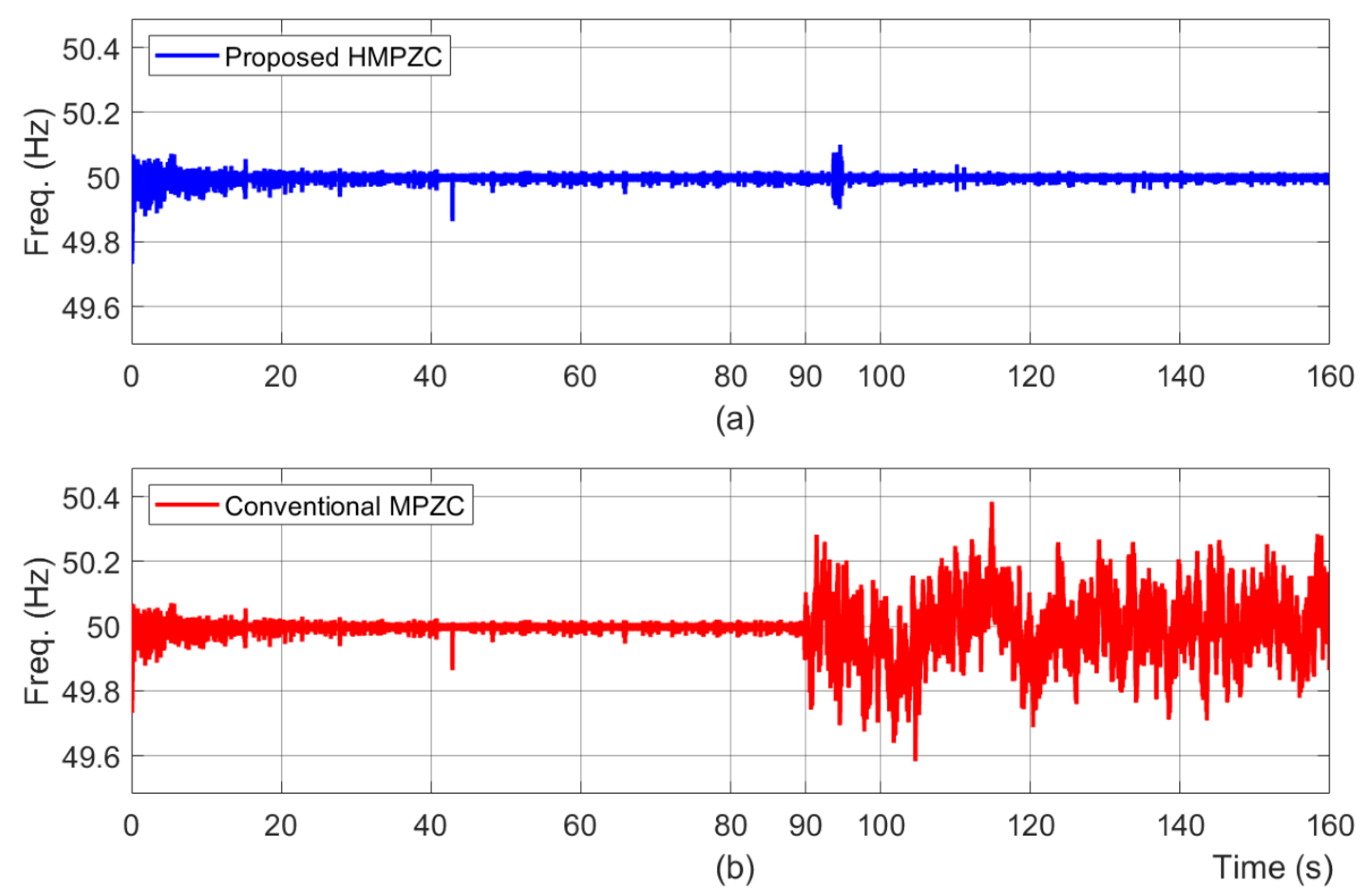
  • From the power, frequency, and voltage characteristics, it is identified that stability is maintained with the HMPZ method, whereas MPZC failed to maintain stability. Unlike T2, this analysis confirms that the HMPZC method has a better chance of enhancing the power delivery capability of the power loop than the conventional MPZC method.
Thus, it is concluded that the proposed HMPZC method has successfully reduced the dq coupling, thereby achieving the enhanced transient response and power delivery capability of the inverters of microgrids.

Author Contributions

Conceptualization, M.S.; Formal analysis, R.M.; Funding acquisition, R.M.; Investigation, C.P.R.; Methodology, Y.V.P.K.; Project administration, C.P.R.; Software, C.P.R.; Supervision, Y.V.P.K.; Validation, R.M.; Visualization, M.S.; Writing—original draft, M.S.; Writing—review and editing, Y.V.P.K. All authors have read and agreed to the published version of the manuscript.

Funding

This work is supported by the Korea Agency for Infrastructure Technology Advancement (KAIA) grant funded by the Ministry of Land, Infrastructure and Transport (Grant RS-2023-00251002).

Data Availability Statement

The original contributions presented in the study are included in the article, further inquiries can be directed to the corresponding author.

Conflicts of Interest

The authors declare no conflicts of interest.

References

  1. IEEE Std 1547-2018; IEEE Standard for Interconnection and Interoperability of Distributed Energy Resources with Associated Electric Power Systems Interfaces. IEEE: Piscataway, NJ, USA, 2018; pp. 1–138. [CrossRef]
  2. Srikanth, M.; Kumar, Y.V.P.; Amir, M.; Mishra, S.; Iqbal, A. Improvement of Transient Performance in Microgrids: Comprehensive Review on Approaches and Methods for Converter Control and Route of Grid Stability. IEEE Open J. Ind. Electron. Soc. 2023, 4, 534–572. [Google Scholar] [CrossRef]
  3. Yu, M.; Huang, W.; Tai, N.; Zheng, X.; Wu, P.; Chen, W. Transient Stability Mechanism of Grid-Connected Inverter-Interfaced Distributed Generators Using Droop Control Strategy. Appl. Energy 2018, 210, 737–747. [Google Scholar] [CrossRef]
  4. Yadav, M.; Jaiswal, P.; Singh, N. Fuzzy Logic-Based Droop Controller for Parallel Inverter in Autonomous Microgrid Using Vectored Controlled Feed-Forward for Unequal Impedance. J. Inst. Eng. India Ser. B 2021, 102, 691–705. [Google Scholar] [CrossRef]
  5. Li, M.; Wang, Y.; Hu, W.; Shu, S.; Yu, P.; Zhang, Z.; Blaabjerg, F. Unified Modeling and Analysis of Dynamic Power Coupling for Grid-Forming Converters. IEEE Trans. Power Electron. 2022, 37, 2321–2337. [Google Scholar] [CrossRef]
  6. Liu, L.; Tian, S.; Xue, D.; Zhang, T.; Chen, Y.; Zhang, S. A Review of Industrial MIMO Decoupling Control. Int. J. Control Autom. Syst. 2019, 17, 1246–1254. [Google Scholar] [CrossRef]
  7. Liu, T.; Zhang, W.; Gu, D. Analytical Design of Decoupling Internal Model Control (IMC) Scheme for Two-Input−Two-Output (TITO) Processes with Time Delays. Ind. Eng. Chem. Res. 2006, 45, 3149–3160. [Google Scholar] [CrossRef]
  8. Wen, T.; Zhu, D.; Zou, X.; Jiang, B.; Peng, L.; Kang, Y. Power coupling mechanism analysis and improved decoupling control for virtual synchronous generator. IEEE Trans. Power Electron. 2021, 36, 3028–3041. [Google Scholar] [CrossRef]
  9. Wen, T.; Zou, X.; Zhu, D.; Guo, X.; Peng, L.; Kang, Y. Comprehensive Perspective on Virtual Inductor for Improved Power Decoupling of Virtual Synchronous Generator Control. IET Renew. Power Gener. 2020, 14, 485–494. [Google Scholar] [CrossRef]
  10. Rathnayake, D.B.; Bahrani, B. Multivariable Control Design for Grid-Forming Inverters with Decoupled Active and Reactive Power Loops. IEEE Trans. Power Electron. 2023, 38, 1635–1649. [Google Scholar] [CrossRef]
  11. Lin, X.; Peng, J.C.-H.; Li, Q.; Cheng, D.; Yu, J.; Wen, H. Power Coupling and Stability Analysis of GFM Due to Rotational Frames and Control Loops Interaction. Int. J. Electr. Power Energy Syst. 2024, 157, 109829. [Google Scholar] [CrossRef]
  12. Haddadi, A.; Yazdani, A.; Joos, G.; Boulet, B. A Gain-Scheduled Decoupling Control Strategy for Enhanced Transient Performance and Stability of an Islanded Active Distribution Network. IEEE Trans. Power Delivery 2014, 29, 560–569. [Google Scholar] [CrossRef]
  13. D’Arco, S.; Suul, J.A.; Fosso, O.B. Automatic Tuning of Cascaded Controllers for Power Converters Using Eigenvalue Parametric Sensitivities. IEEE Trans. Ind. Appl. 2015, 51, 1743–1753. [Google Scholar] [CrossRef]
  14. Yazdanian, M.; Mehrizi-Sani, A. Case Studies on Cascade Voltage Control of Islanded Microgrids Based on the Internal Model Control. IFAC-PapersOnLine 2015, 48, 578–582. [Google Scholar] [CrossRef]
  15. Fu, X.; Li, S. A Novel Neural Network Vector Control for Single-Phase Grid-Connected Converters with L, LC and LCL Filters. Energies 2016, 9, 328. [Google Scholar] [CrossRef]
  16. Yazdanian, M.; Mehrizi-Sani, A. Internal Model-Based Current Control of the RL Filter-Based Voltage-Sourced Converter. IEEE Trans. Energy Convers. 2014, 29, 873–881. [Google Scholar] [CrossRef]
  17. Leitner, S.; Yazdanian, M.; Mehrizi-Sani, A.; Muetze, A. Small-Signal Stability Analysis of an Inverter-Based Microgrid with Internal Model-Based Controllers. IEEE Trans. Smart Grid 2018, 9, 5393–5402. [Google Scholar] [CrossRef]
  18. Pavan Kumar, Y.V.; Bhimasingu, R. Design of Voltage and Current Controller Parameters Using Small Signal Model-Based Pole-Zero Cancellation Method for Improved Transient Response in Microgrids. SN Appl. Sci. 2021, 3, 836. [Google Scholar] [CrossRef]
  19. Srikanth, M.; Venkata Pavan Kumar, Y. PSO Based Modified Pole-Zero Cancellation Technique for VSI Control to Improve Transient Response in Microgrids. Int. J. Renew. Energy Res. 2024, in press.
  20. Comanescu, M.; Xu, L.; Batzel, T.D. Decoupled Current Control of Sensorless Induction-Motor Drives by Integral Sliding Mode. IEEE Trans. Ind. Electron. 2008, 55, 3836–3845. [Google Scholar] [CrossRef]
  21. Rohten, J.A.; Dewar, D.N.; Zanchetta, P.; Formentini, A.; Muñoz, J.A.; Baier, C.R.; Silva, J.J. Multivariable Deadbeat Control of Power Electronics Converters with Fast Dynamic Response and Fixed Switching Frequency. Energies 2021, 14, 313. [Google Scholar] [CrossRef]
  22. Junior, R.S.R.; Machado, E.P.; Júnior, D.F. Development of a multivariable deadbeat controller in dq coordinates for the current loop of a grid-connected VSI. J. Control Autom. Electr. Syst. 2024, 35, 588–600. [Google Scholar] [CrossRef]
  23. Holmes, D.G.; McGrath, B.P.; Parker, S.G. Current Regulation Strategies for Vector-Controlled Induction Motor Drives. IEEE Trans. Ind. Electron. 2012, 59, 3680–3689. [Google Scholar] [CrossRef]
  24. Babaei, S.; Parkhideh, B.; Chandorkar, M.C.; Fardanesh, B.; Bhattacharya, S. Dual Angle Control for Line-Frequency-Switched Static Synchronous Compensators Under System Faults. IEEE Trans. Power Electron. 2014, 29, 2723–2736. [Google Scholar] [CrossRef]
  25. Amézquita-Brooks, L.A.; Licéaga-Castro, J.; Licéaga-Castro, E.; Ugalde-Loo, C.E. Induction Motor Control: Multivariable Analysis and Effective Decentralized Control of Stator Currents for High-Performance Applications. IEEE Trans. Ind. Electron. 2015, 62, 6818–6832. [Google Scholar] [CrossRef]
  26. Bahrani, B.; Kenzelmann, S.; Rufer, A. Multivariable-PI-Based dq Current Control of Voltage Source Converters with Superior Axis Decoupling Capability. IEEE Trans. Ind. Electron. 2011, 58, 3016–3026. [Google Scholar] [CrossRef]
  27. Ashabani, M.; Mohamed, Y.A.-R.I.; Mirsalim, M.; Aghashabani, M. Multivariable Droop Control of Synchronous Current Converters in Weak Grids/Microgrids with Decoupled Dq-Axes Currents. IEEE Trans. Smart Grid 2015, 6, 1610–1620. [Google Scholar] [CrossRef]
  28. Ghasemi, M.A.; Zarei, S.F.; Peyghami, S.; Blaabjerg, F. A Theoretical Concept of Decoupled Current Control Scheme for Grid-Connected Inverter with L-C-L Filter. Appl. Sci. 2021, 11, 6256. [Google Scholar] [CrossRef]
  29. Gopi Krishna Rao, P.V.; Subramanyam, M.V.; Satyaprasad, K. Design of Internal Model Control-Proportional Integral Derivative Controller with Improved Filter for Disturbance Rejection. Syst. Sci. Control. Eng. 2014, 2, 583–592. [Google Scholar] [CrossRef]
  30. Woldeamanuel, L.H.; Ramaveerapathiran, A. Design of Multivariable PID Control Scheme for Humidity and Temperature Control of Neonatal Incubator. IEEE Access 2024, 12, 6051–6062. [Google Scholar] [CrossRef]
  31. Touqan, B.; Abdul, A.A.; Salameh, M. HVAC multivariable system modelling and control. Proc. Inst. Mech. Eng. Part C J. Mech. Eng. Sci. 2023, 237, 2049–2061. [Google Scholar] [CrossRef]
  32. Luan, X.; Chen, Q.; Liu, F. Equivalent Transfer Function Based Multi-Loop PI Control for High Dimensional Multivariable Systems. Int. J. Control Autom. Syst. 2015, 13, 346–352. [Google Scholar] [CrossRef]
  33. Ogunba, K.S.; Fakunle, A.A.; Ogunfunmi, T.; Taiwo, O. Extended Approach to Analytical Triangular Decoupling Internal Model Control of Square Stable Multivariable Systems with Delays and Right-Half-Plane Zeros. IEEE Access 2023, 11, 32201–32228. [Google Scholar] [CrossRef]
  34. Liu, K.; Chen, J. Internal Model Control Design Based on Equal Order Fractional Butterworth Filter for Multivariable Systems. IEEE Access 2020, 8, 84667–84679. [Google Scholar] [CrossRef]
  35. Chekari, T.; Mansouri, R.; Bettayeb, M. Improved Internal Model Control-Proportional-Integral-Derivative Fractional-Order Multiloop Controller Design for Non Integer Order Multivariable Systems. J. Dyn. Syst. Meas. Control 2019, 141, 011014. [Google Scholar] [CrossRef]
  36. Skogestad, S. Simple Analytic Rules for Model Reduction and PID Controller Tuning. J. Process Control 2003, 13, 291–309. [Google Scholar] [CrossRef]
  37. Azar, A.T.; Serrano, F.E. Robust IMC–PID Tuning for Cascade Control Systems with Gain and Phase Margin Specifications. Neural Comput. Appl. 2014, 25, 983–995. [Google Scholar] [CrossRef]
  38. Ramezani, M.; Li, S.; Sun, Y. Combining Droop and Direct Current Vector Control for Control of Parallel Inverters in Microgrid. IET Renew. Power Gener. 2017, 11, 107–114. [Google Scholar] [CrossRef]
  39. Kumar, Y.V.P.; Bhimasingu, R. Fuzzy Logic Based Adaptive Virtual Inertia in Droop Control Operation of the Microgrid for Improved Transient Response. In Proceedings of the 2017 IEEE PES Asia-Pacific Power and Energy Engineering Conference (APPEEC), Bangalore, India, 8–10 November 2017; IEEE: Piscataway, NJ, USA, 2017; pp. 1–6. [Google Scholar] [CrossRef]
  40. Rocabert, J.; Luna, A.; Blaabjerg, F.; Rodríguez, P. Control of Power Converters in AC Microgrids. IEEE Trans. Power Electron. 2012, 27, 4734–4749. [Google Scholar] [CrossRef]
Figure 1. Layout diagram of the microgrid model under study.
Energies 17 03689 g001
Figure 2. Model of the multiloop control structure.
Energies 17 03689 g002
Figure 3. Block diagram for design of (a) CCL and (b) VCL.
Energies 17 03689 g003
Figure 4. Flow chart for finding the optimum integral constant of the forward path controller in the VCL using the PSO.
Energies 17 03689 g004
Figure 5. Model of conventional and proposed methodologies.
Energies 17 03689 g005
Figure 6. Typical feedback control system.
Energies 17 03689 g006
Figure 7. IMC design for the feedback control system.
Energies 17 03689 g007
Figure 8. Model for design of CCL.
Energies 17 03689 g008
Figure 9. Model for design of VCL.
Energies 17 03689 g009
Figure 10. Block diagram of CCL with (a) conventional MPZC and (b) proposed HMPZC.
Energies 17 03689 g010
Figure 11. Open-loop CCL Bode plot with (a) conventional MPZC and (b) proposed HMPZC.
Energies 17 03689 g011
Figure 12. Closed-loop CCL Bode plot with (a) conventional MPZC and (b) proposed HMPZC.
Energies 17 03689 g012
Figure 13. Effect of step input in d-axis on d-axis output in (a) conventional MPZC and (b) proposed HMPZC.
Energies 17 03689 g013
Figure 14. Effect of step input in d-axis on q-axis output in (a) conventional MPZC and (b) proposed HMPZC.
Energies 17 03689 g014
Figure 15. Frequency results under test case T1. (a) proposed HMPZC; (b) conventional MPZC; (c) zoomed portion of the results at 80 s; (d) zoomed portion of the results at 90 s.
Energies 17 03689 g015
Figure 16. Active power results under test case T1. (a) proposed HMPZC; (b) conventional MPZC.
Energies 17 03689 g016
Figure 17. Voltage results under test case T1. (a) proposed HMPZC; (b) conventional MPZC; (c) zoomed portion of proposed HMPZC result at 90 s; (d) zoomed portion of conventional MPZC result at 90 s.
Energies 17 03689 g017
Figure 18. Voltage THD results for test case T1: (a) Proposed HMPZC and (b) conventional MPZC.
Energies 17 03689 g018
Figure 19. Frequency results under test case T2. (a) proposed HMPZC; (b) conventional MPZC; (c) zoomed portion of the results at 80 s; (d) zoomed portion of the results at 90 s.
Energies 17 03689 g019aEnergies 17 03689 g019b
Figure 20. Active power results under test case T2. (a) proposed HMPZC; (b) conventional MPZC.
Energies 17 03689 g020
Figure 21. Voltage results under test case T2. (a) proposed HMPZC; (b) conventional MPZC; (c) zoomed portion of proposed HMPZC result at 90 s; (d) zoomed portion of conventional MPZC result at 90 s.
Energies 17 03689 g021
Figure 22. Voltage THD results for test case T2: (a) Proposed HMPZC and (b) conventional MPZC.
Energies 17 03689 g022
Figure 23. Frequency results under test case T3. (a) proposed HMPZC; (b) conventional MPZC.
Energies 17 03689 g023
Figure 24. Active power results under test case T3. (a) proposed HMPZC; (b) conventional MPZC.
Energies 17 03689 g024
Figure 25. Voltage results under test case T3. (a) proposed HMPZC; (b) conventional MPZC; (c) zoomed portion of proposed HMPZC result at 90 s; (d) zoomed portion of conventional MPZC result at 90 s.
Energies 17 03689 g025
Figure 26. Voltage THD for test case T3: (a) Proposed HMPZC, (b) conventional MPZC.
Energies 17 03689 g026
Table 1. Summary of different test cases.
Test CaseLoad 1
(kW + jkVar)
Load 2
(kW + jkVar)
Operating Power Factor
0–80 s80–90 s90–160 s
T11.2 + j0.30.3 + j3.50.970.370.97
T21.2 + j0.30.3 + j5.00.970.270.97
T31.2 + j0.30.3 + j8.00.970.180.97
Table 2. Summary of various control parameters and their values.
ParameterDescriptionMPZCHMPZC
TITime constant of GIplant(s)10 × 10−310 × 10−3
TPWM1/switching frequency5 × 10−45 × 10−4
DpMaximum P-ω droop gain of the APL1 × 10−41 × 10−4
DqMaximum Q-v droop gain of the RPL1.48 × 10−31.48 × 10⁻³
KIp,fProportional gain in the forward path of the CCL’s PI controller0.120.12
KIi,fIntegral gain in the forward path of the CCL’s PI controller0.8 × 1030.8 × 103
KVp,fProportional gain in the forward path of the VCL’s PI controller5.65 × 10−45.65 × 10⁻⁴
KVi,fIntegral gain in the forward path of the VCL’s PI controller0.2480.248
KIp,ccProportional gain in the cross-coupling path of CCL’s PID controller0.314 (ωoL)31.42 × 10⁻⁵
KIi,ccIntegral gain in the cross-coupling path of the CCL’s PID controllerNA0.3142
KId,ccDerivative gain in cross-coupling path of CCL’s PID controllerNA0
KVp,ccProportional gain in the cross-coupling path of VCL’s PID controller0.0016 (ωoC)15.7
KVi,ccIntegral gain in cross-coupling path of VCL’s PID controllerNA7.85 × 103
KVd,ccDerivative gain in cross-coupling path of VCL’s PID controllerNA0
Table 3. Transient response comparison of the proposed HMPZC and conventional MPZC schemes.
Performance CharacteristicsTest CaseCorresponding to Load Switching at t = 80 sCorresponding to Load Switching at t = 90 s
Conv. MPZC
[18,19]
Prop. HMPZCSuperior MethodConv. MPZC
[18,19]
Prop. HMPZCSuperior Method
Frequency characteristics
Desired:
  • Deviation: ≤0.05 Hz (IEEE 1547)
Max. deviation during overshoot (Hz)T100Both0.0150.010HMPZC
T20.0010Both0.0200.020Both
T30.0050.004HMPZC0.4000.025HMPZC
Max. deviation during undershoot (Hz)T10.0020.002Both0.0400.007HMPZC
T20.0020.002Both0.0500.009HMPZC
T30.0030.003Both0.4000.017HMPZC
Power characteristics
Desired:
  • System stability: Stable
  • Extra burden: low

System stability (Stable/Unstable)T1StableStableBothStableStableBoth
T2StableStableBothStableStableBoth
T3StableStableBothUnstableStableHMPZC
Extra burden (Watts)T115291308HMPZC851613HMPZC
T223071914HMPZC1114928HMPZC
T360834751HMPZC19521845HMPZC
Voltage characteristics
  • Desired THD: <5%
THD (%)T1NCNC--3.493.08HMPZC
T2NCNC--5.623.33HMPZC
T3NCNC--20.23.39HMPZC
Disclaimer/Publisher’s Note: The statements, opinions and data contained in all publications are solely those of the individual author(s) and contributor(s) and not of MDPI and/or the editor(s). MDPI and/or the editor(s) disclaim responsibility for any injury to people or property resulting from any ideas, methods, instructions or products referred to in the content.

