Abstract
The current power load exhibits strong nonlinear and stochastic characteristics, increasing the difficulty of short-term prediction. To more accurately capture data features and enhance prediction accuracy and generalization ability, in this paper, we propose an efficient approach for short-term electric load forecasting that is grounded in a synergistic strategy of feature optimization and hyperparameter tuning. Firstly, a dynamic adjustment strategy based on the rate of the change of historical optimal values is introduced to enhance the PID-based Search Algorithm (PSA), enabling the real-time adjustment and optimization of the search process. Subsequently, the proposed Improved Population-based Search Algorithm (IPSA) is employed to achieve the optimal adaptive variational mode decomposition of the load sequence, thereby reducing data volatility. Next, for each load component, a Bi-directional Gated Recurrent Unit network with an attention mechanism (BiGRU-Attention) is established. By leveraging the interdependence between feature selection and hyperparameter optimization, we propose a synergistic optimization strategy based on the Improved Population-based Search Algorithm (IPSA). This approach ensures that the input features and hyperparameters for each component’s predictive model achieve an optimal combination, thereby enhancing prediction performance. Finally, the optimal parameter prediction model is used for multi-step rolling forecasting, with the final prediction values obtained through superposition and reconstruction. The case study results indicate that this method can achieve an adaptive optimization of hybrid prediction model parameters, providing superior prediction accuracy compared to the commonly used methods. Additionally, the method demonstrates robust adaptability to load forecasting across various day types and seasons. Consequently, this approach enhances the accuracy of short-term load forecasting, thereby supporting more efficient power scheduling and resource allocation.
1. Introduction
Short-term power load forecasting involves predicting the electrical load for upcoming hours to days, serving as a crucial foundation for power dispatch operations [1]. Influenced by multiple factors such as meteorology and social activities, load data exhibit strong nonlinearity and randomness, significantly increasing the difficulty and complexity of short-term forecasting [2]. Hence, to ensure the safe and stable operation of power systems, there is an urgent need to explore and integrate innovative methodologies and technologies that can enhance prediction accuracy and stability, thereby precisely meeting the stringent requirements of the engineering technology domain.
Current short-term electric load forecasting methods primarily encompass traditional mathematical statistics, machine learning, and hybrid approaches. Traditional methods are well-suited for predicting smooth and highly periodic sequences but exhibit poor performance with highly stochastic loads. Machine learning techniques, including support vector machines [3], artificial neural networks [2], and deep learning [4,5], have gained prominence. In recent years, Recurrent Neural Networks (RNNs) have demonstrated exceptional performance in the field of load forecasting. Long Short-Term Memory (LSTM) neural networks and Gated Recurrent Unit (GRU) neural networks are representative models of the RNN [6]. Among them, GRU simplifies the gating structure of LSTM, reducing the number of parameters and accelerating convergence [7]. Among these, the Gated Recurrent Unit (GRU) neural network is widely adopted for its exceptional capability in handling time-series signals and its relatively simple structure. However, GRU models consider only forward information in sequences, neglecting reverse correlation [8]. To address this limitation, the Bidirectional Gated Recurrent Unit (BiGRU) model has been introduced and has found extensive application in load forecasting. Ref. [9] introduces a short-term power load forecasting technique that integrates convolutional neural networks with BiGRU. The results indicate that the BiGRU network enhances prediction accuracy and more effectively captures long-term dependencies and temporal dynamic features compared to unidirectional GRU networks. Despite the advantages of deep learning methods over traditional approaches, their performance is influenced by data quality, quantity, and model hyperparameters. This poses a persistent challenge for a single model in pursuing optimal prediction outcomes, making it difficult to ensure stable performance.
With the increasing complexity of load data, hybrid forecasting methods that integrate data processing techniques and forecasting models have emerged. These data processing techniques include load series decomposition and correlation analysis of load-influencing factors. Concurrently, to enhance model generalization ability and reduce the complexity of parameter determination, many researchers have incorporated intelligent algorithm optimization into the data processing techniques of hybrid forecasting models and the hyperparameter optimization process. Current sequence decomposition techniques primarily include discrete wavelet transform, Empirical Mode Decomposition (EMD) [10], Ensemble Empirical Mode Decomposition (EEMD) [11], and Variational Mode Decomposition (VMD) [12]. EMD addresses the issue of needing to preset the wavelet basis and the order of the wavelet, but suffers from prominent mode aliasing problems [10]. EEMD mitigates mode aliasing by introducing white noise but leaves residual noise that adversely affects modal decomposition [11]. Ref. [13] has demonstrated that VMD can avoid mode aliasing and improve the prediction accuracy of load components; however, its key parameters are often determined through numerous experiments, leading to suboptimal decomposition effects. Therefore, Ref. [14] presents an adaptive VMD method enhanced by the sparrow optimization algorithm, which, despite its potential, suffers from slow convergence and a propensity to fall into local optimum [15]. Furthermore, the hyperparameters of the prediction model are typically determined through multiple trials, limiting the enhancement of prediction performance. Ref. [16] proposed a hybrid prediction model based on sequence component reorganization and a temporal self-attention mechanism. This method employs the central frequency method to determine the number of VMD components, demonstrating the advantages of combining VMD technology with deep learning models for prediction. However, it did not address the critical impact of hyperparameter optimization on model performance. Therefore, it is evident that incorporating VMD technology in hybrid prediction models is notably advantageous, and the prediction models must include efficient optimization algorithms to maximize prediction efficiency and model generalization capability.
Most existing prediction methods rely on multivariate input feature sets to mine data features. However, an excessive number of features can significantly burden model convergence, adversely affecting prediction performance. Therefore, analyzing the correlation of load-influencing factors and downscaling the input features is crucial [14]. Refs. [17,18] utilized the conditional mutual information method and the maximal information coefficient method, respectively, to select optimal features. However, both approaches overlooked the consideration of redundancy among the influencing factors of the load, resulting in redundant features that reduced prediction accuracy and increased computational burden. Ref. [19] describes the minimum Redundancy Maximum Relevance (mRMR) algorithm, which is designed to select feature subsets that are highly relevant to the target while minimizing redundancy. Refs. [20,21] introduced mRMR into the selection of input feature sets for load forecasting and used the fruit fly optimization algorithm and the improved particle swarm optimization algorithm to optimize network hyperparameters, thereby enhancing prediction performance. However, these methods determine the optimal number of features through multiple trials aimed at minimizing prediction error, resulting in computational inefficiency and unstable outcomes. Ref. [22] employs an improved particle swarm optimization algorithm to determine the optimal number of features for the mRMR algorithm, yet the prediction model’s hyperparameters are still determined through multiple trials, rendering the model less adaptive. It is evident that the existing studies seldom consider the interdependence between feature selection and model hyperparameter determination. Both sets of parameters are typically determined using traditional meta-heuristic optimization algorithms and manual test methods, without employing a synergistic determination approach. Furthermore, traditional meta-heuristic optimization algorithms face challenges such as poor population diversity, low search accuracy, and slow convergence speed [23], which limit the model’s prediction efficiency and generalization ability.
In summary, current deep-learning forecasting methods are significantly influenced by data quality, quantity, and model hyperparameters. Most prediction models determine hyperparameters through multiple trials or optimize them using traditional meta-heuristic algorithms with low search precision and slow convergence speeds, resulting in limited performance improvement. Additionally, multivariate input feature sets increase the training burden on the model, and the existing studies seldom consider the interdependence between feature selection and model hyperparameters. To enhance the performance of forecasting models, this paper proposes a short-term electric load forecasting method based on a BiGRU-Attention network structure. This method integrates feature selection and hyperparameter co-optimization, enabling the adaptive adjustment of model hyperparameters and the efficient identification of optimal parameters, thereby reducing the complexity and uncertainty of manual trials. This approach also leverages the synergistic effects of various components in the hybrid prediction model, achieving optimal forecasting performance. The contributions and innovations of this paper are as follows:
- A dynamic adjustment strategy based on the rate of the change of the historical optimal value is proposed to realize that the Improved PSA (IPSA) algorithm can adaptively adjust the PID parameters in real time during the search process. In comparison to conventional meta-heuristic optimization algorithms, this algorithm can strike a balance between search speed and stability and has a higher success rate of searching for optimal values and a faster convergence speed.
- The IPSA algorithm is successively applied to optimize the parameters of variational mode decomposition and to conduct a two-stage synergistic optimization strategy, focusing on the selection of the original load feature set and hyperparameter settings to improve prediction accuracy. This approach efficiently achieves an adaptive variational mode decomposition of the original load sequence and determines the optimal combination of input feature sets and hyperparameters for each load component.
- A multi-step rolling prediction strategy is implemented for each component, and the prediction results of each component are superimposed and reconstructed to obtain the final result. The prediction results based on the actual electricity load dataset in Australia show that the method in this paper can realize the efficient tuning of the parameters in each stage of the hybrid prediction model, and the accuracy is significantly improved compared with the commonly used methods, which is more adaptable to the load prediction of different day types and seasons.
2. Materials and Methods
2.1. Improved Algorithm for PSA
2.1.1. PSA Algorithm
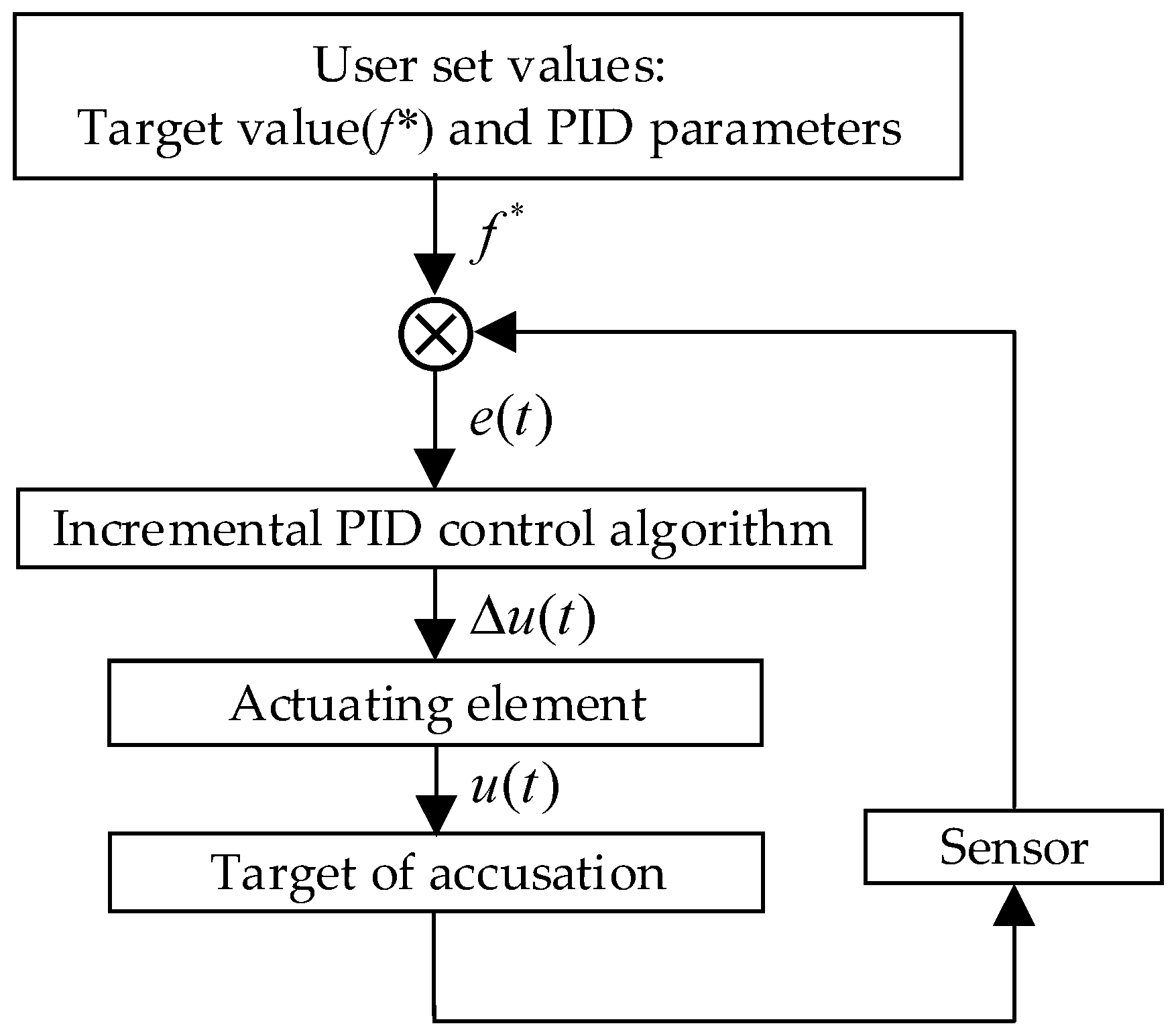
The PID-based Search Algorithm (PSA) [24], introduced by Yuansheng Gao in 2023, is a metaheuristic optimization algorithm designed to explore global optimal solutions. It emulates the regulation process of incremental PID control (Figure 1) and updates particle positions based on the increment of the control quantity, thereby enabling the population to converge efficiently to the optimal state. The PSA algorithm demonstrates superior accuracy and stability compared to common intelligent optimization algorithms. The execution process of the algorithm comprises four main components: population initialization, deviation computation, dynamic adjustment of PID parameters, and position update.

Figure 1.
The adjustment process of incremental PID control.
- Population Initialization
In a D-dimensional search space, there are N particles, with the upper and lower bounds of the search range in the j-th dimension denoted as and respectively. In the PSA algorithm, the random initial position of each particle can be represented as , and the objective function value of the i-th particle is given in (1), where r is a random number in the range [0, 1]. The PSA control parameters include the maximum number of iterations, T, and the population size, N.
- 2.
- Calculation of Population Bias
The position update of the population in the PSA algorithm is inspired by the incremental PID algorithm. During the population evolution process, the historically optimal individual is designated as the target reference point for the optimization process, while each particle represents the actual value. The position of each particle is updated by calculating the deviation of the population and adjusting the incremental control quantity accordingly. The incremental control quantity at time t, denoted as , is the difference between the control quantities at time t and the previous time step t − 1, i.e., as shown in (2). The detailed derivation process can be found in Appendix A.
where , , and are the proportional, integral, and derivative coefficients, respectively. The term denotes the deviation between the setpoint and the actual value at time t.
During the PSA optimization process, the optimal individual at the t-th iteration, denoted as , corresponds to the historically best value of the population. At this point, the deviation of the population individual is given by:
Let the population deviation of the previous iteration and the previous two iterations at the first iteration be and , respectively. Then when , it is possible to make . Additionally, when , since the objective value of the PSA algorithm is the historical optimum that changes with iterations. Therefore, in the PSA algorithm is not equal to the deviation at the t1st iteration, and in the PSA algorithm can be expressed as Equation (4), the derivation of which is described in Ref. [24].
where is the historically optimal individual at the tth iteration, and is the historically optimal individual at the t1st iteration.
- 3.
- Population Individual Position Updates
To enhance the algorithm’s randomness and global search capability, multiple random numbers are introduced in the calculation of the output increment of the PID regulation in the PSA algorithm, which is expressed as follows:
where , , and are N × 1 random vectors with values ranging from 0 to 1. The parameters , , and are typically fixed values set manually, requiring repeated trials and adjustments to optimize their performance [24].
Additionally, to prevent the controlled object from becoming unresponsive when the deviation value is zero, the PID algorithm often adds a constant to the deviation value. However, this approach may cause the PSA algorithm to become confined to a local optimum during the early iterations. Therefore, the PSA algorithm incorporates a zero-output adjustment factor based on . The zero-output adjustment factor is defined as:
where is an N × D random vector with values ranging from 0 to 1; T denotes the maximum number of iterations; L represents a Lévy flight function, with its calculation formula provided in Ref. [24]; is an adjustment coefficient, defined as:
As t increases, decreases slowly, which aids the algorithm in thoroughly exploring the search space. In the later stages, decreases rapidly, prompting the algorithm to utilize existing information rather than extensively explore new solutions.
The PSA algorithm updates the population of individuals based on and , with the update formula defined as:
In this equation, is a N × 1 matrix, expressed as:
where is an N × 1 random matrix with values ranging from 0 to 1.
2.1.2. Improved PSA Algorithm Based on Dynamic Regulation Strategy
In the PSA algorithm, PID parameters are typically fixed, which may not effectively meet system demands, especially for complex nonlinear systems. The process of determining these parameters is time-consuming and labor-intensive, heavily relying on the experience and expertise of the operator. To address these issues, this paper proposes the Improved PSA (IPSA) algorithm, which incorporates a dynamic adjustment strategy for PID parameters based on the rate of the change of the historical optimal function values. This approach modifies the calculation method for the PID-controlled output increment, , within the PSA algorithm.
The dynamic adjustment strategy introduces the historical optimal function value change rate factor, ξ, allowing , , and to vary with the optimization process. This enables the algorithm to more flexibly adapt to different scenarios and the demands of complex systems. The improved formula for the PID-controlled output increment, , is as follows:
where the original parameters , , and are replaced by the sums of their initial values , , and the factor ξ. The factor ξ is defined as follows:
The variation rate of the historical optimal function value indicates the present optimization state and the trend of its historical changes. When the rate of change is high, it indicates that the population is in a highly optimized state. In this case, PID parameters should be appropriately increased to accelerate the optimization process. Conversely, when the rate of change is low, PID parameters should be decreased to avoid oscillations and ensure convergence to the optimal solution.
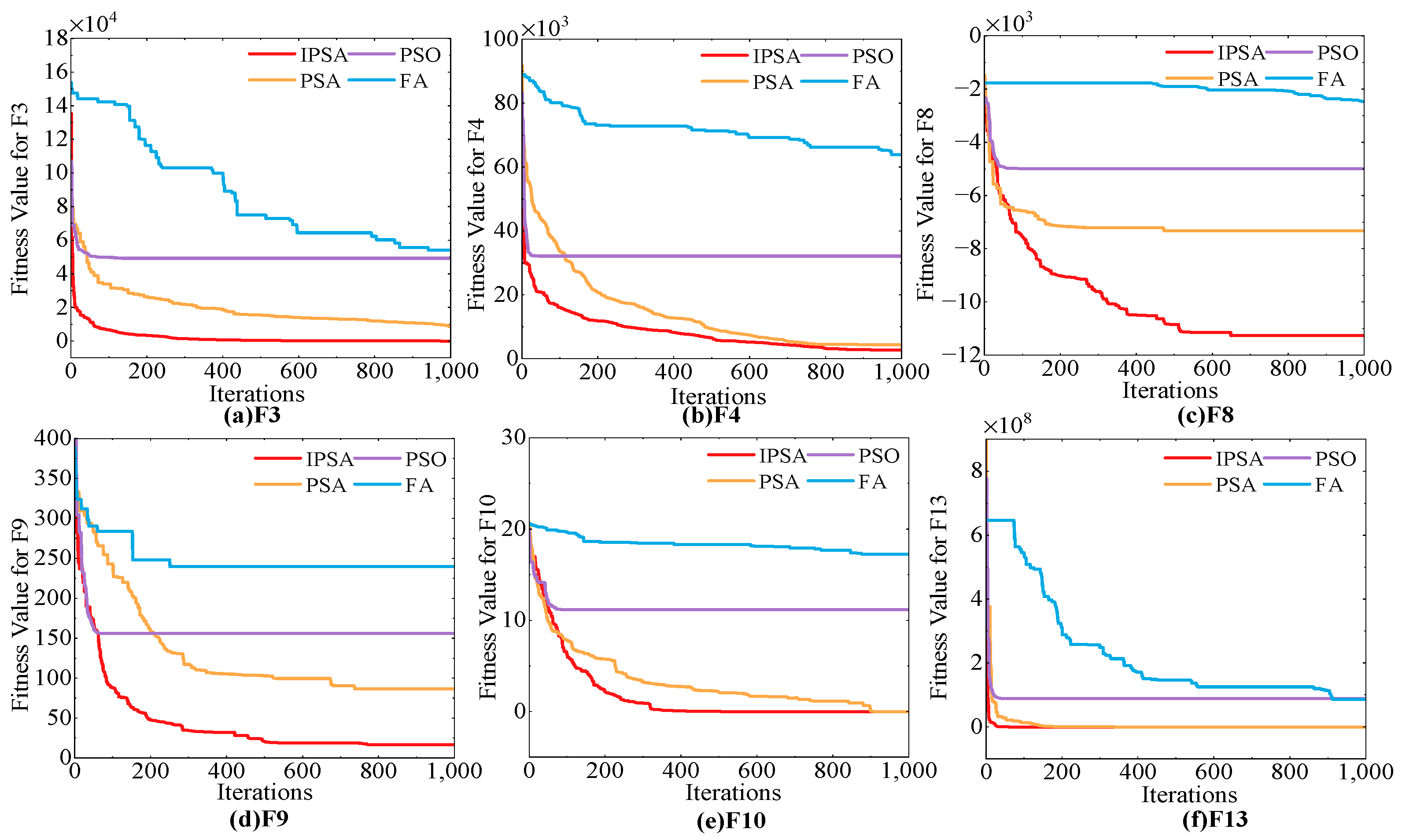
The execution flow of the IPSA algorithm is shown in Table A1. We tested IPSA, PSA, and two other common optimization algorithms on six benchmark functions from CEC2017. The population size was established at 50, with the maximum number of iterations set to 1000. The outcomes of the tests are presented in Figure 2. Experimental data indicate a gradual increase in the number of iteration rounds, the IPSA algorithm demonstrates the highest optimization success rate and faster convergence speed. Furthermore, the probability of the IPSA algorithm falling into a local optimum is significantly reduced, making it more stable compared to the other three algorithms.
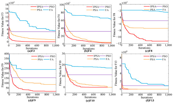
Figure 2.
Fitness curves of four algorithms for six benchmark functions in CEC2017.
Based on these findings, this paper introduces the IPSA algorithm to the optimization of key VMD parameters, as well as the co-optimization of feature selection and model hyperparameters.
2.2. Adaptive Variational Mode Decomposition
2.2.1. Variational Mode Decomposition
The VMD technique enhances the accuracy of load forecasting by reducing complexity through the decomposition of the original load sequence and the construction of independent prediction models for each component. VMD, as a completely non-recursive modal decomposition technique, defines the modal components as amplitude and frequency modulation functions and aims to decompose the signal into a small number of k narrow-bandwidth intrinsic modal functions . The bandwidth of is given by:
where represents the k-th modal component post-decomposition; is the center frequency of the modal components; δ(t) is the unit pulse function. The Lagrange multiplier and the second-order penalty coefficient α are introduced in Equation (12), and the generalized Lagrangian expression is given by:
The Alternating Direction Method of Multipliers (ADMMs) is used to solve Equation (13), continuously updating each component and its center frequency is as follows:
where the Wiener filter and frequency center are denoted as and , respectively.
2.2.2. Adaptive Variational Modal Decomposition Based on IPSA
Unlike the EMD and EEMD algorithms, the VMD algorithm requires pre-setting the number of mode components K and the penalty coefficient α. The value of K affects the degree of decomposition, while α influences the completeness of the retained information. Therefore, determining the optimal combination of [K, α] is crucial for load modal decomposition. Given the complex and variable nature of actual power load signals, manually setting K and α can introduce uncertainties and be time-consuming, often leading to unstable decomposition results [25].
To address this, the paper utilizes the IPSA algorithm, as detailed in Section 2.1.2, to optimize the critical parameters of VMD. This approach allows VMD to dynamically adjust parameters based on the characteristics of the actual data, facilitating the identification of the optimal [K, α] parameter combination in a shorter time frame.
To avoid mode mixing and ensure the optimal extraction of load decomposition information without loss, thereby aiding the predictive model in better understanding the periodic variations of complex load data, this paper sets the optimization objective function to minimize energy entropy [23]:
In Equation (16), , Where N represents the length of the time series data and denotes the amplitude of the time series information.
To determine the optimal parameter combination [K, α] for the adaptive VMD algorithm using the IPSA algorithm, the following steps are employed:
- (1)
- Configure the parameters of the IPSA algorithm and initialize the population, taking the energy entropy as the objective function.
- (2)
- Decompose the signal using VMD and evaluate the objective function values for each individual using Equation (16).
- (3)
- Compare the objective function values of the individuals, compute the population deviation, update the minimum objective function value, and update the positions of the population individuals according to the IPSA algorithm.
- (4)
- Continue iterating through steps (2) and (3) until the global objective function value reaches the minimization or the maximum iteration count is reached. Finally, output the optimal parameters [K, α].
2.3. Feature Optimization and Model Hyperparameter Co-Tuning Methods
2.3.1. mRMR Algorithm
Due to the adverse impact of correlation and redundancy among multiple features on prediction accuracy, and the increased burden on model convergence, this paper introduces the mRMR (Minimum Redundancy Maximum Relevance) algorithm for selecting input feature sets for each component prediction model. This ensures that the input features for each component maximize the correlation with the load sequence while minimizing the redundancy among features.
The mRMR algorithm evaluates the dependency between features using mutual information. The mutual information between variables and is expressed as Equation (17), where , , and are the probability densities and joint probability density of and , respectively.
According to the definition of mutual information, maximum relevance can be represented by Equation (18), while minimum redundancy is expressed by Equation (19).
In Equations (18) and (19), S denotes the feature set; is the dimension; I(xi, c) is the mutual information between feature xi and the target c; I(xi, xj) is the mutual information between xi and xj. Additionally, D and R stand for relevance and redundancy, respectively.
The mRMR algorithm can be represented by Equations (18) and (19) as follows:
To solve Equation (20), an incremental search algorithm is employed [18]. When adding the n-th feature to the n − 1 feature set selected from the original feature set X, it should satisfy:
2.3.2. BiGRU Model Based on Attention Mechanism
The GRU is derived from the simplified gated structure of the LSTM network. LSTM includes forget gates, input gates, and output gates, making it a type of recurrent neural network capable of capturing long-term dependencies [6]. To reduce the number of parameters and effectively avoid the problem of gradient explosion, the GRU combines the forget gate and input gate of LSTM into a single update gate. The GRU model includes both update and reset gates. The update gate regulates the degree to which previous state information is preserved in the current state, capturing short-term dependencies in the time series; the reset gate decides whether to integrate the current state with prior information, capturing long-term dependencies.
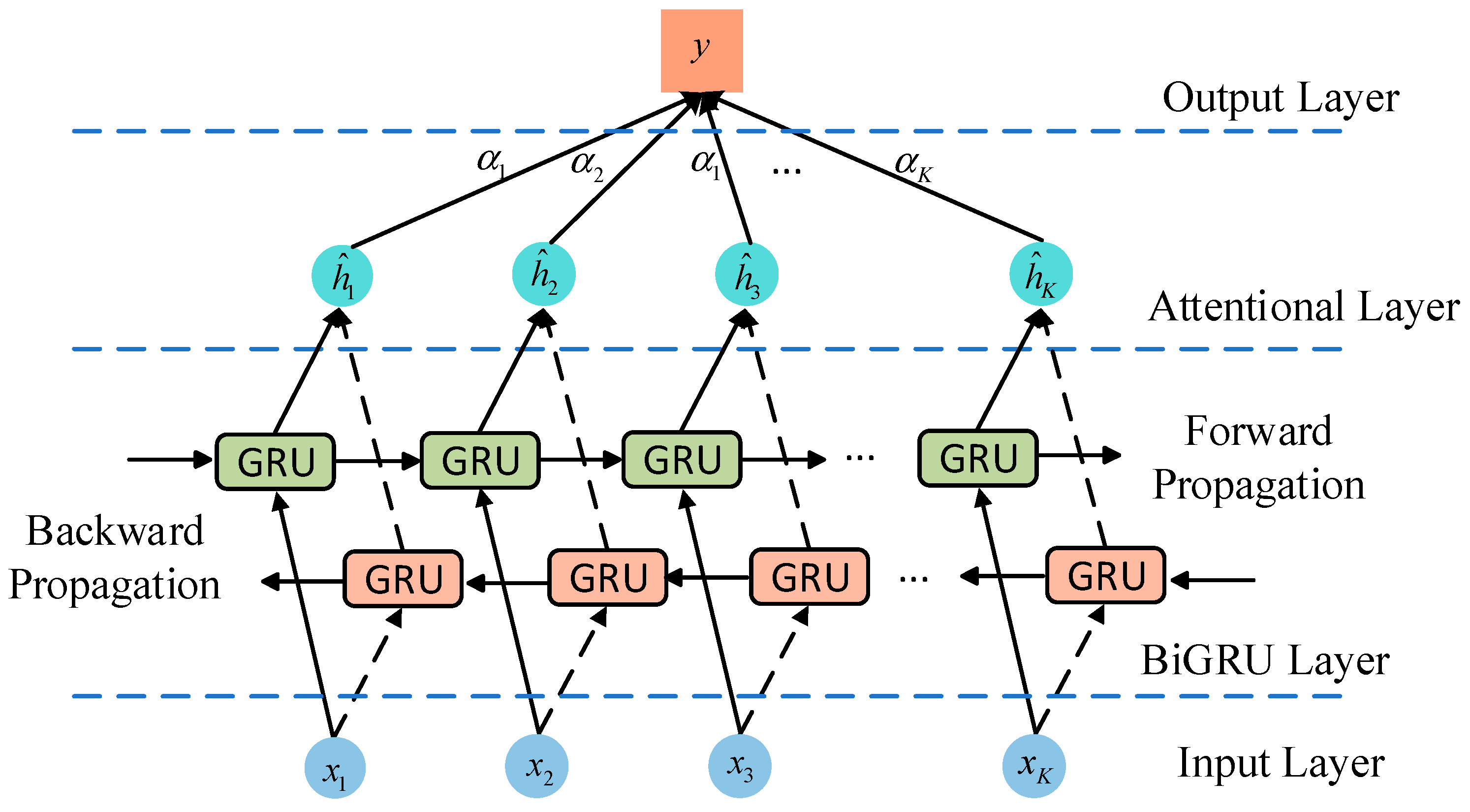
To comprehensively extract temporal features from all input samples, this paper introduces the Bidirectional GRU (BiGRU) model. The BiGRU model consists of two GRU units propagating in opposite directions: one learns future data during forward propagation, while the other learns historical data during backward propagation. However, BiGRU may face challenges such as information loss and modeling difficulties when dealing with long sequences due to information overload. To address this limitation, we incorporate an attention mechanism following the BiGRU layer. The attention mechanism assigns probability weights to the hidden states of the BiGRU network, allowing the model to focus more on key parts relevant to the task and enhancing the influence of important information. The weight coefficients for the attention layer are calculated using the following formula:
where eij represents the attention weight between positions i and j; αij is the attention weight obtained by normalizing eij; and si is the output of the attention layer obtained by weighting the hidden state according to αij. Finally, the prediction y is obtained through a fully connected layer.
Figure 3 illustrates the structure of the BiGRU-Attention model.
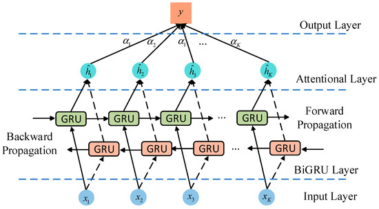
Figure 3.
Structure diagram of attention mechanism.
2.3.3. Methods of Co-Tuning Feature Optimization and Hyperparameter Based on IPSA
When using the mRMR algorithm to select the best input features for each modal component from the original feature set X, determining the number of features in the subset (N0) is a critical step. The number of features affects the input dimensionality of the model, thereby influencing the complexity and training process of the model, which leads to varying model performance [18].
Typically, the method for determining N0 involves comparing the prediction accuracy under different N0 values while keeping the model structure and its hyperparameters fixed. This helps to identify the optimal number of features N0 for each component. However, this approach requires testing the model’s prediction accuracy for each N0 value individually, resulting in long prediction times, low efficiency, and poor adaptability.
Simultaneously, the setting of hyperparameters is crucial for accelerating model convergence, reducing overfitting, and improving model generalization performance. When determining model hyperparameters, optimizing the number of optimal features independently overlooks the interdependence between optimal feature selection and hyperparameter determination. Different optimal hyperparameters may correspond to different optimal feature sets, and vice versa.
Specifically, when selecting feature sets, the redundancy and correlation among features can impact the training process of the model. For instance, the mRMR algorithm selects features that are highly relevant but have low redundancy, optimizing the feature set. Different optimal feature sets can alter the shape of the model’s loss function, thereby affecting the best settings for the hyperparameters. Consequently, different input feature sets require specific hyperparameter configurations to achieve optimal performance and uncover the intrinsic patterns of the data. In the case of high-dimensional feature sets, higher regularization parameters might be more appropriate to prevent overfitting, while low-dimensional feature sets may need lower regularization parameters to fully utilize the feature information. Moreover, the hyperparameter tuning process can influence the selection of the optimal feature set. For example, if a higher learning rate is chosen, a more compact and significant feature set is needed to ensure stable training of the model. Conversely, a lower learning rate requires a richer feature set to fully learn the patterns within the data. Thus, it is evident that the configuration of optimal hyperparameters needs to be tailored to the specific input feature set to maximize its effectiveness.
In summary, ignoring the interdependent relationship between optimal feature selection and hyperparameter determination can result in suboptimal prediction outcomes. This oversight prevents the identification of the best combination of feature subsets and hyperparameters, ultimately affecting the performance of the model.
Furthermore, common hyperparameter-search algorithms, such as grid search, are often time consuming and inefficient. They also exhibit imbalanced optimization performance for discrete variables (such as the number of neurons and hidden layers) and continuous variables (such as learning rate and dropout rate) [26].
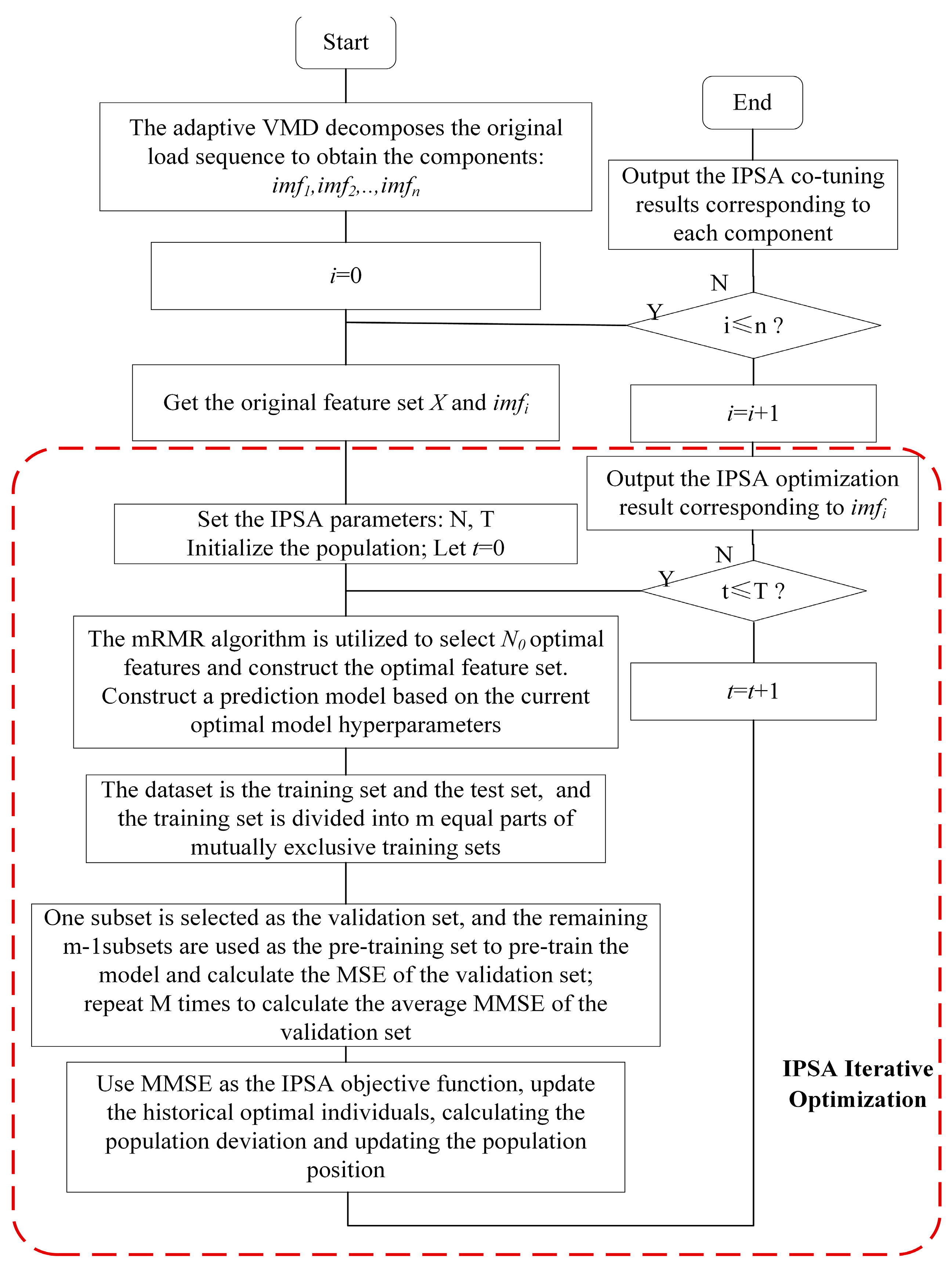
To address these issues, this paper proposes a cooperative optimization method for feature selection and hyperparameter tuning based on the IPSA algorithm. This method aims to efficiently optimize the number of features in the mRMR feature selection algorithm and the model hyperparameters simultaneously to achieve the optimal model performance. The flowchart for the cooperative optimization of feature selection and hyperparameter tuning for each component is shown below:
As shown in Figure 4, this paper incorporates a cross-validation strategy based on the IPSA algorithm to enhance the efficiency of parameter optimization for the prediction model. This strategy involves randomly partitioning the dataset into m mutually exclusive subsets. In each iteration, m − 1 subsets are used for training, while the remaining subset is used for validation. This process is repeated m times, with performance metrics computed for each validation. The average of these metrics is then taken as the evaluation result of the model.
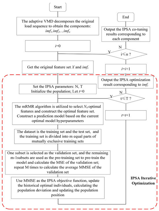
Figure 4.
Flowchart of collaborative optimization of feature selection and model hyperparameters.
The parameters to be optimized in this model include the optimal number of features for each component, the length of the hidden layers in each BiGRU layer, the learning rate, the batch size, and the dropout rate. The mean square error (MSE) average is used as the objective function to update the historical best individual, calculate population deviation and its function value, and update the positions of population individuals according to the IPSA algorithm.
This method integrates the critical steps of feature selection and model optimization, aiming to leverage the synergy between feature selection and hyperparameters. It ensures that the feature selection and model hyperparameters for each component achieve optimal performance. This approach enables the model to more accurately capture data characteristics, thereby reducing the complexity and uncertainty of manual trials, enhancing the model’s adaptability, and improving prediction efficiency and accuracy.
3. Short-Term Power Load Hybrid Prediction Model
3.1. Structure of the Short-Term Power Load Hybrid Prediction Model
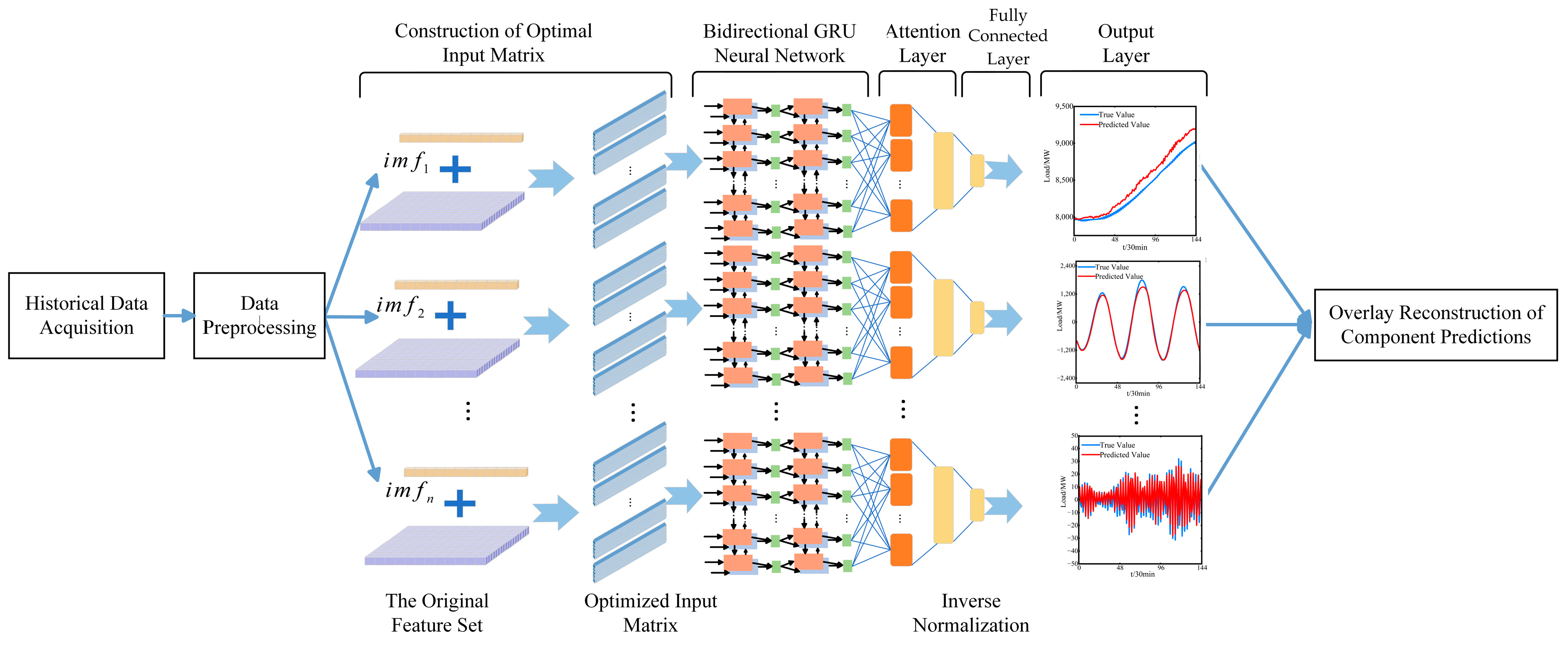
This paper proposes a short-term power load forecasting method based on the synergistic optimization of feature selection and hyperparameters. The method comprises five parts: data collection, data preprocessing and adaptive VMD, IPSA algorithm-assisted optimization of mRMR feature selection and BiGRU-Attention network hyperparameters, optimal parameter model training and prediction, and the reconstruction of the prediction results by summing the components. This model combines the load data processing techniques of the hybrid prediction model with the hyperparameter optimization of the prediction model, enabling the prediction model to more accurately capture data characteristics and enhancing the accuracy of the output layer of the prediction model. The construction process is as follows:
Step 1: Historical Data Acquisition: In this study, the original feature set for short-term power load prediction is constructed from four aspects: calendar features, meteorological impact features, real-time electricity price features, and historical load features.
Step 2: Data Preprocessing: To mitigate the non-stationary nature of power load data, the adaptive mode decomposition method from Section 2.2.2 is utilized to optimally decompose the preprocessed historical power load data into n narrow-bandwidth IMF (Intrinsic Mode Function) components. Simultaneously, each component is normalized.
Step 3: The Establishment of Initial Optimal Input Matrices for Each Mode Component: For each mode component, initial optimal input matrices are established, incorporating component information and the initial optimal feature set. The BiGRU-Attention prediction model structure is also defined.
Step 4: Synergistic Optimization of Model Parameters: Using the IPSA algorithm-based feature selection and model hyperparameter synergistic optimization method from Section 2.3.3, the parameters to be optimized are fine-tuned to obtain the optimal combination of features and hyperparameters.
Step 5: Training with Optimal Parameters: Based on the optimal parameter combination obtained in Step 4, the optimal input matrices for each mode component and the BiGRU-Attention prediction model with optimal hyperparameters are constructed and trained. In the model training process, the Mean Squared Error (MSE) is utilized as the loss function, and the Adam algorithm is employed for adaptive-learning-rate-based weight updates.
Step 6: Prediction Results: Multi-step rolling forecasts are conducted using the trained models for each component. The predicted results for all components are inverse-normalized and aggregated to reconstruct the final prediction result.
The model’s overall structure is depicted in Figure 5. The predictive model consists of five layers: an input layer, a bidirectional GRU layer, an attention mechanism layer, a fully connected layer, and an output layer.
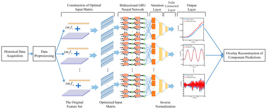
Figure 5.
Diagram of short-term power load forecasting method based on feature selection and co-optimization of hyperparameters.
3.2. Evaluation Indicators for the Model
The predictive performance of the model is evaluated using four metrics: Root Mean Square Error (RMSE), Mean Absolute Error (MAE), Mean Absolute Percentage Error (MAPE), and Explained Variance Score (EV). Among these, RMSE, MAE, and MAPE reflect prediction accuracy, with smaller values indicating higher accuracy. EV represents the proportion of the variance in the target variable explained by the prediction model, with values closer to 1 indicating a stronger explanatory power and better model fit. The formulas for calculating RMSE, MAE, MAPE, and EV are as follows:
where N represents the number of samples, and represent the true and predicted values at time t, respectively, and νar() denotes the variance.
4. Case Studies
Short-term load forecasting utilizes actual power load data sourced from New South Wales, Australia, focusing on industrial loads from 1 March 2007 to 29 February 2008. The dataset is divided into four original datasets based on seasons, with each season serving as a dataset. The final week of each season serves as the testing set, and the remaining data are partitioned into training and validation sets, with the validation set constituting 20% of the training data.
The construction of the original feature set is crucial for load forecasting, significantly influencing model simplification, training time, applicability, and prediction outcomes. Based on the existing empirical knowledge, electricity loads exhibit daily and weekly cycles. In this study, historical input features for the model primarily consist of the past 7 days’ features at the forecasted time and the previous 24 hours’ data on load, weather, electricity prices, and calendar events. Additionally, considering the predictability of meteorological forecasts for the forecast day and the availability of calendar features, both are included as known information inputs to the prediction model. The future load at all time points of the forecast day serves as the output for the prediction model. Details of the dataset features are provided in Table 1.

Table 1.
Dataset features.
4.1. Data Preprocessing and Model Construction
4.1.1. Load Sequence Decomposition and Normalization
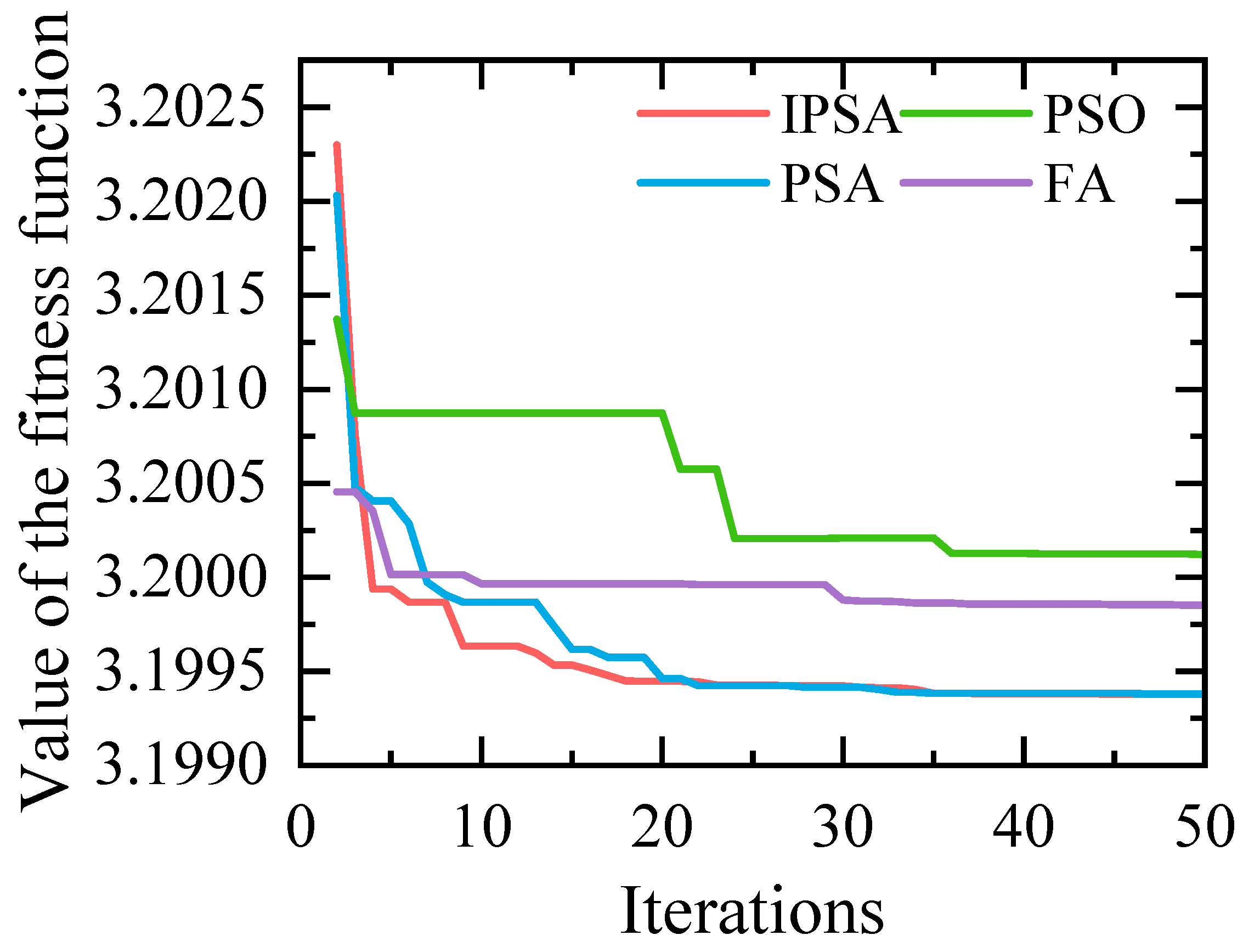
Using spring season data as an example, the objective function variation curves for VMD parameter optimization under different optimization algorithms are depicted in Figure 6. Compared to three other algorithms, the Improved Population-based Search Algorithm (IPSA)achieves the fastest optimization speed and yields lower fitness values. The population size for all optimization algorithms is set to 50, with 50 iterations and search ranges of K ∈ [3, 10] and α ∈ [500, 3000]. Initial values for parameters [Kp, Ki, Kd] in IPSA and PSA algorithms are set to [1, 0.5, 1.2] [24].
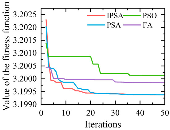
Figure 6.
Fitness curve of adaptive VMD optimized by different algorithms.
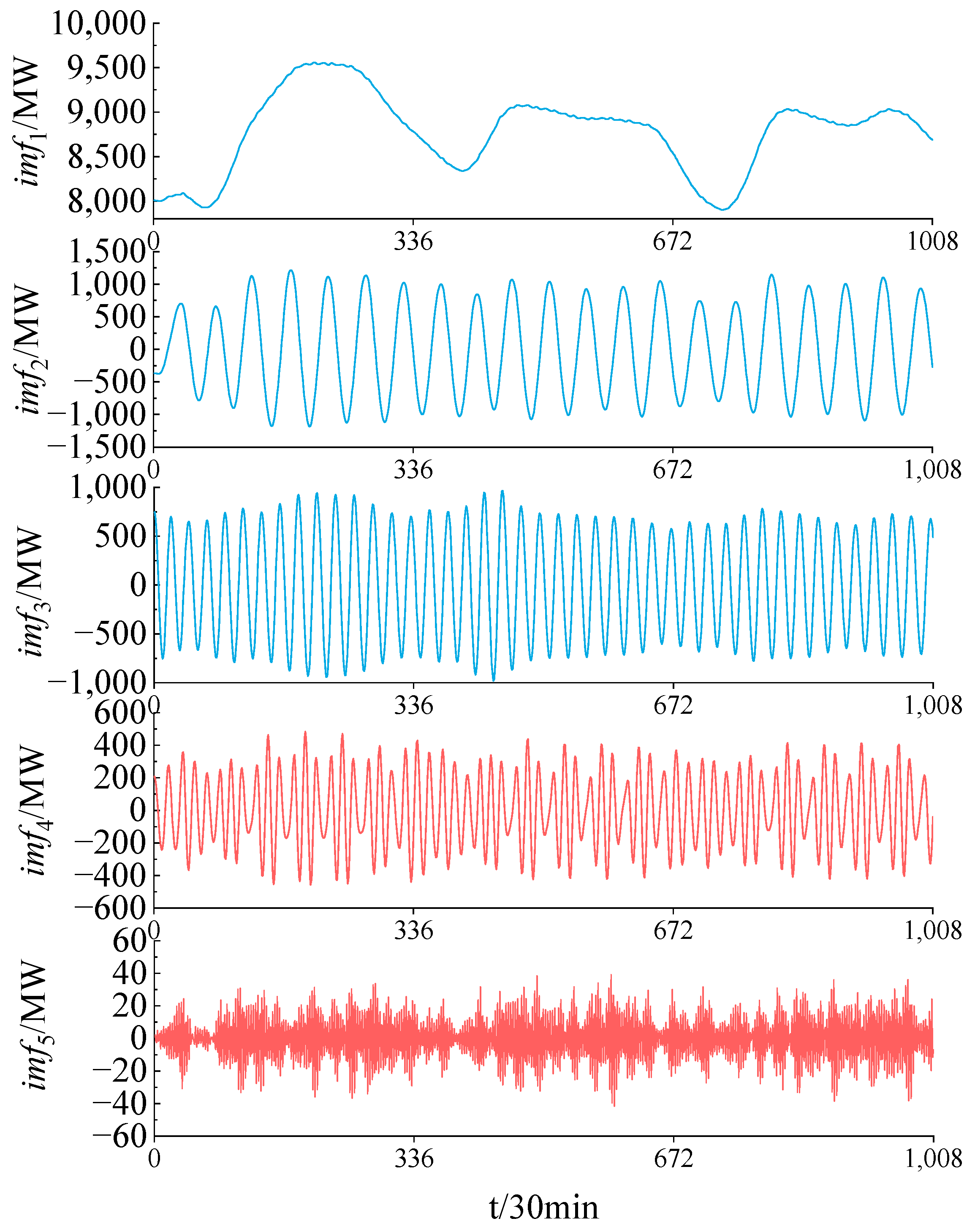
Using the adaptive variational mode decomposition method detailed in Section 2.2.2, the optimal parameter combination [K, α] is determined as [5, 2240]. The results of the sample sequence decomposition are shown in Figure 7. It is evident from the images of imf1 to imf3 that the sample sequence exhibits weekly and daily periodicity, while imf4 and imf5 capture non-stationary, high-frequency components within the sample sequence.
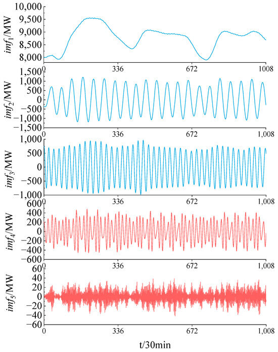
Figure 7.
Partial results of adaptive VMD load sequence decomposition.
The numerical differences among the components after VMD are substantial. Directly inputting these into the prediction model could distort the overall mapping effect. Therefore, we perform z-score normalization on the decomposed sequences, with the calculation formula as follows:
4.1.2. Model Selection Comparison
This study compares the proposed model with three common types of models:
- Type I Models: Single prediction models considering load temporal characteristics, including LSTM, GRU, and BiGRU accounting for bidirectional temporal features, and BiGRU-Attention neural networks. These models capture the temporal features of load data using a single neural network.
- Type II Models: Hybrid prediction methods integrating load data processing techniques with prediction models. This includes EEMD-BiGRU and VMD-BiGRU. These models first decompose the raw load data, and then combine it with prediction models.
- Type III Models: Hybrid prediction models that incorporate model hyperparameter optimization and attention mechanisms, based on Particle Swarm Optimization (PSO) [10] for EEMD-BiGRU-Attention and Firefly Algorithm (FA) for VMD-mRMR-BiGRU-Attention. PSO and FA are used to optimize model hyperparameters, while the attention mechanism enhances the model’s ability to capture important features. By selecting these three types of models as benchmarks, this study comprehensively demonstrates the performance advantages of the proposed model in load forecasting and validates the effectiveness of the proposed method under different data processing and model optimization techniques.
All models use the Mean Squared Error (MSE) as the loss function, and the Adam algorithm is employed for weight parameter optimization. All models have two hidden layers, a batch size of 256, 50 training epochs, and a prediction step size of 48 [27]. The Mean Squared Error (MSE) is used as the loss function, and the Adam algorithm is employed for weight optimization. A 5-fold cross-validation strategy is applied. The input features include the entire original feature set (Table 2). For hyperparameter optimization, both T and N are set to 30 and 50, respectively, with the optimization algorithm’s objective function being the Minimization of MSE (MMSE).
Table 2.
IPSA algorithm parameter settings and collaborative optimization parameter search range settings.
The parameter settings for the comparison prediction models are shown in Table A2. The hyperparameters for the first and second types of comparison models are determined using grid search. The hyperparameter determination for the proposed model is detailed in Section 4.1.3.
4.1.3. Input Feature Matrix and Prediction Model Construction
Using spring season data as an example, the optimal input matrix and model hyperparameters for each component are optimized using the IPSA-based feature selection and hyperparameter co-optimization method described in Section 2.3.3. The parameter settings for the IPSA algorithm and the search ranges for the parameters to be optimized are provided in Table 2.
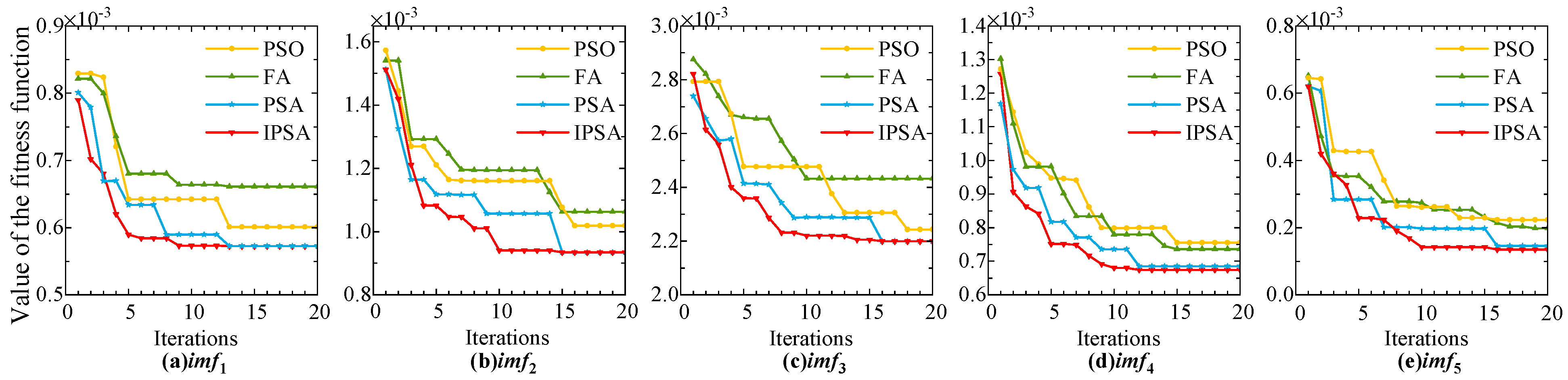
Figure 8 shows the objective function variation curves for the prediction model parameters of each component under different optimization algorithms. Compared to the other three algorithms, the IPSA algorithm demonstrates the fastest optimization speed, as well as superior optimization capability and adaptability during the feature selection and hyperparameter co-optimization process.
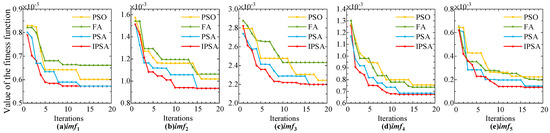
Figure 8.
Variation curve of objective function for parameter optimization of each component prediction model.
Table 3 presents the optimal hyperparameters for the prediction models of each component, determined using the IPSA-based feature selection and hyperparameter co-optimization method.
Table 3.
Optimization results of hyperparameters for each component prediction model.
Table 4 lists the optimal number of features and the optimal feature set for each component as determined by the IPSA-based method. It is evident that the imf1 component is influenced by various features, such as historical load, real-time temperature and humidity values, electricity prices at the same time as the previous week, and day type. The imf2 and imf3 components are mainly influenced by the historical load at the same time as the previous week, real-time temperature and humidity, time of day, and day type. The imf4 and imf5 components are primarily influenced by the historical load at the same time as the previous week.
Table 4.
Optimal input features for each component.
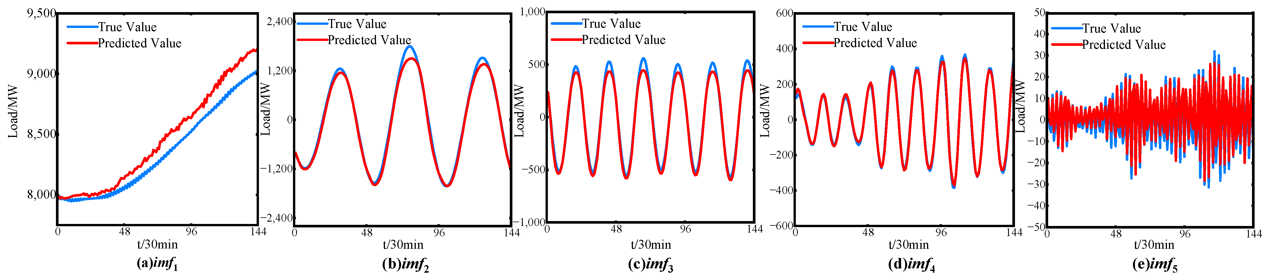
Figure 9 shows the partial prediction results of each component of the spring load using the proposed prediction method. Overall, the predicted values of each component closely match the actual load curve, indicating a good prediction performance.
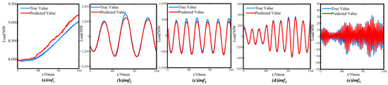
Figure 9.
Spring load prediction results for each component.
4.2. Prediction Performance Validation and Comparison
4.2.1. Comparison of Predicted Results with Actual Load Curves
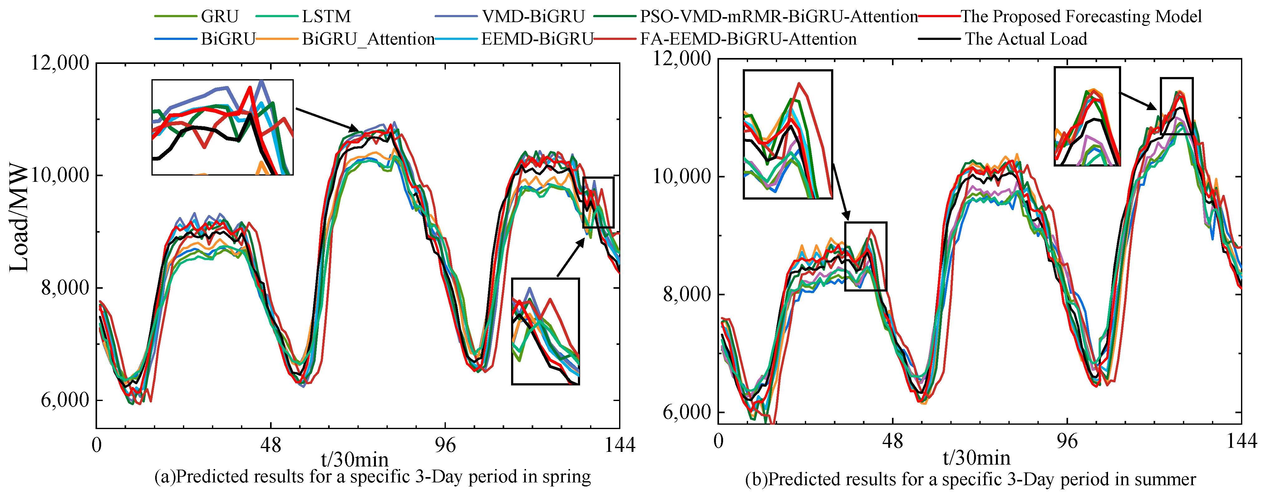
Figure 10 illustrates the load forecasting results of various models for three test days in spring and summer, compared to the actual load curves. The figure shows that the proposed forecasting model more closely aligns with the actual load curves overall. The magnified sections in Figure 8 indicate that the proposed model performs well in capturing the true load values during periods of significant load fluctuations and peak–valley segments.
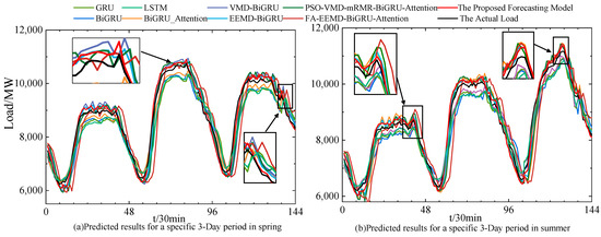
Figure 10.
Prediction results and actual load curve.
4.2.2. Comparison of Prediction Performance with Baseline Models
Figure 11 presents the results of the four evaluation metrics, RMSE, MAE, MAPE, and EV, for the proposed prediction model and three comparison models on the sample test set. Compared to all the comparison models, the proposed model reduced RMSE, MAE, and MAPE on the test set by 129.97 MW, 99.59 MW, and 0.92%, respectively. These findings indicate that the proposed forecasting model significantly improves the accuracy of short-term power load forecasts and exhibits robust fitting capabilities for actual load curves characterized by strong nonlinearities.
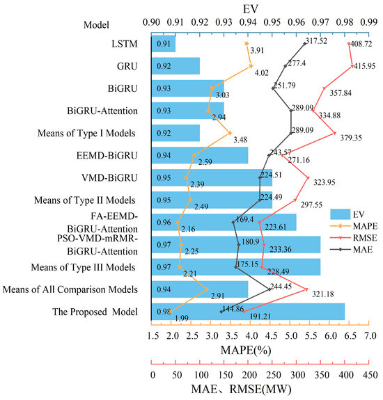
Figure 11.
Evaluation metrics of different prediction models.
Compared to the Type I Models of single predictive models that account for the load temporal characteristics, the Type II Models, which combine load processing techniques with predictive models, show significant improvements in the test set. Specifically, the average RMSE, MAE and MAPE of the Type II Models decrease by 81.80 MW, 64.60 MW, and 0.99%, respectively, and the EV value increases by 0.03. Notably, the VMD-GRU model, when compared to the GRU model in the second category, reduces the RMSE, MAE, and MAPE by 92.00 MW, 47.11 MW, and 1.63%, respectively. Moreover, our proposed model demonstrates a substantial reduction in the average RMSE, MAE, and MAPE by 188.13 MW, 144.23 MW, and 1.48%, respectively, and an increase in EV value by 0.06 compared to the first category models. These comparisons validate that models combining load sequence decomposition, prediction, and reconstruction structures, or integrating input feature selection algorithms with single predictive models, effectively enhance prediction performance and accuracy. Specifically, load sequence decomposition algorithms help models to better capture periodicity and trends in data, while input feature selection algorithms help to reduce noise and redundant information, improving the model’s generalization ability and prediction accuracy.
In comparison with the Type II Models of hybrid predictive models, the Type III Models introduce neural network hyperparameter optimization and the attention mechanism. Experimental results indicate that, compared to the Type II Models, the Type III Models reduced the average RMSE, MAE, and MAPE by 69.06 MW, 49.35 MW, and 0.28%, respectively, and increased the EV value by 0.02. Compared to the Type II Models, the proposed model reduced the average RMSE, MAE, and MAPE by 106.34 MW, 76.64 MW, and 0.50%, respectively, and increased the EV value by 0.03. These results confirm that the introduction of hyperparameter optimization algorithms in predictive models allows for automatic adjustment of model hyperparameters, reducing human factor influences. Optimal hyperparameter settings and the attention mechanism improve the model’s representation and prediction accuracy for load data, thus optimizing model performance.
Compared to the Type III Models of hybrid models that only optimize neural network hyperparameters, our proposed model employs the IPSA algorithm not only to optimize the number of components in the Variational Model Decomposition algorithm (VMD)but also to conduct collaborative optimization during feature selection and model hyperparameter determination stages. Compared to the Type III Models, the proposed model reduced the average RMSE, MAE, and MAPE by 37.28 MW, 30.29 MW, and 0.22%, respectively, and increased the EV value by 0.01. This demonstrates that integrating feature engineering and model optimization into key steps allows for collaborative optimization aimed at improving the prediction accuracy for each component after load sequence decomposition. Optimizing the predictive model parameters enhances the model’s ability to extract load data features, which is crucial for improving prediction accuracy and performance. Additionally, using high-performance optimization algorithms, such as the IPSA algorithm, for predictive model parameter optimization enhances the model’s adaptability.
4.2.3. Adaptability to Different Seasons and Days
Table 5 presents the evaluation metrics for the prediction results of different models on weekdays and weekends in the test set. From Table 5, it is evident that the models demonstrate higher prediction accuracy for weekends compared to weekdays. Compared to weekdays, the average RMSE, MAE, and MAPE of all benchmark models decreased by 378.54 MW, 21.94 MW, and 0.22%, respectively, on weekends, while the EV value increased by 0.02. This improvement is attributed to the higher proportion of industrial load during weekends. In contrast, compared to the other benchmark models, the proposed model demonstrated a greater improvement in predictive accuracy. For weekdays, the average RMSE, MAE, and MAPE decreased by 137.77 MW, 103.59 MW, and 0.97%, respectively, while for weekends, these metrics decreased by 122.17 MW, 94.71 MW, and 0.86%, respectively. Additionally, the average EV value for weekdays remained above 0.97. These results demonstrate that our model exhibits strong adaptability in load prediction tasks across different day types.
Table 5.
Evaluation metrics of prediction models for different daily types.
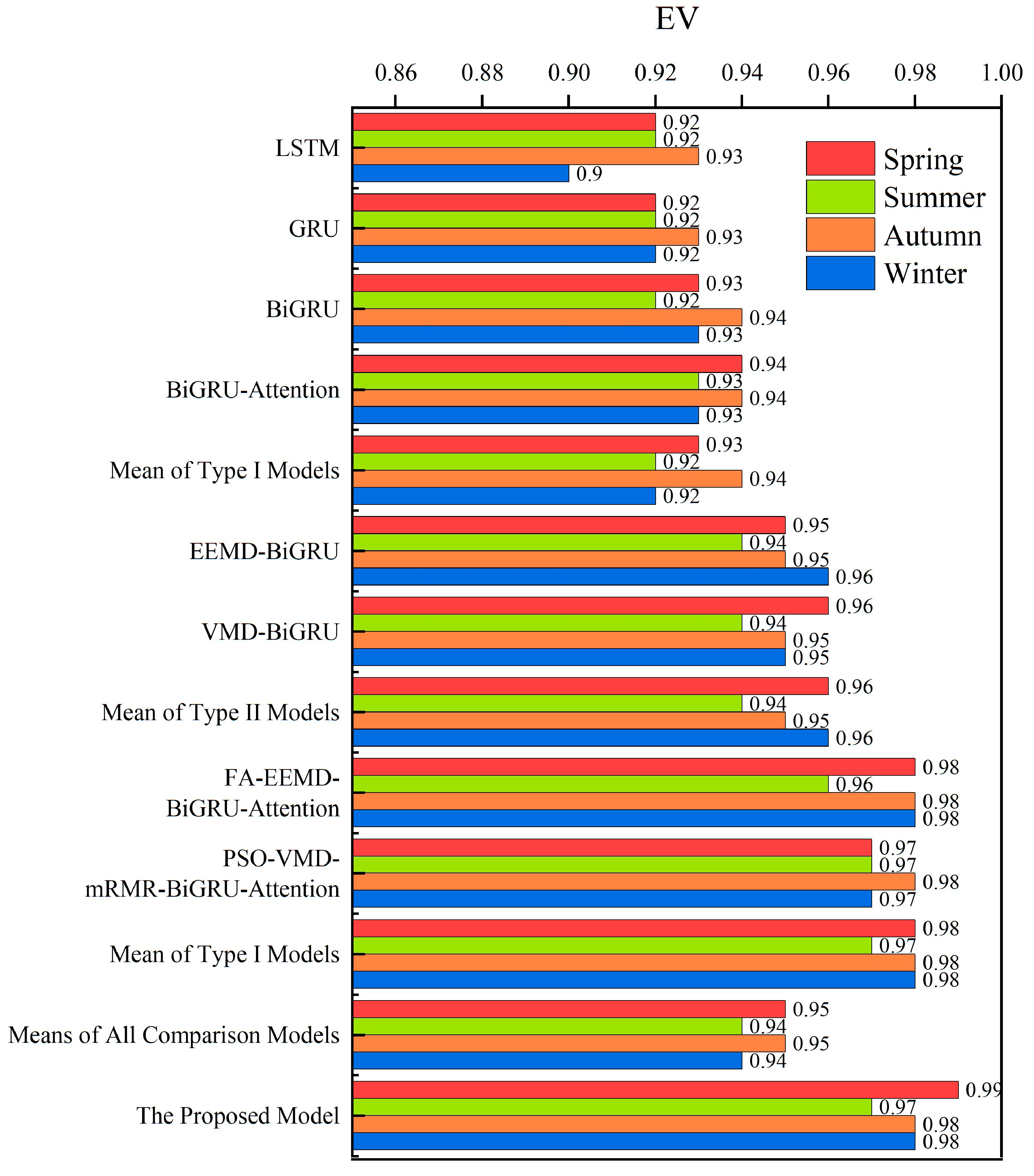
As shown in Table 6 and Figure 12, the performance of the prediction models varies across different seasonal test sets. The prediction accuracy is highest for autumn and lowest for summer. Compared to summer, the autumn prediction model’s RMSE, MAE, and MAPE are reduced by 12.06 MW, 5.42 MW, and 0.09%, respectively. This is due to the increased average load demand and the larger fluctuations in peak load periods during summer, which makes prediction more challenging. In contrast, for the proposed model, the RMSE, MAE, and MAPE are the lowest across all four seasons, with the EV value consistently above 0.97. This indicates that our model maintains high prediction accuracy and performance, demonstrating strong adaptability across different seasons.
Table 6.
Evaluation metrics of prediction models for different seasons.

Figure 12.
EV values of the prediction models for different seasons.
5. Conclusions
This paper leverages the advantages of intelligent optimization algorithms and data processing techniques, integrating them with predictive models to propose a hybrid method for short-term electric load forecasting. The proposed method is validated using a real-world dataset, primarily composed of highly volatile industrial load data. The conclusions are as follows:
- (1)
- The dynamic adjustment strategy for PID parameters based on the rate of the change of historical optimal function values proposed in this study improves the convergence speed and adaptability of the Improved Population-based Simulated Annealing (IPSA) algorithm. This lays a foundation for enhancing the optimization performance of the forecasting method.
- (2)
- By integrating the IPSA optimization algorithm into adaptive variational mode decomposition, as well as coordinated optimization of feature selection and model hyperparameters, the method efficiently searches for optimal solutions, achieving optimal values for parameters at each stage of the prediction model. This approach effectively utilizes the interdependence between feature selection and model hyperparameters, enhancing the capture of data characteristics, while reducing the need for manual intervention and its impact.
The IPSA optimization algorithm is introduced into the adaptive variational mode decomposition and the synergistic optimization of input feature selection and model hyperparameters. This approach enables the rapid identification of the optimal solutions for load sequence decomposition, feature selection, and model hyperparameters. As a result, the model can fully exploit the interdependence between load input features and hyperparameters, further capturing load data characteristics while minimizing the need for and impact of manual intervention.
- (3)
- Compared to the conventional methods, the proposed approach reduces forecasting complexity and demonstrates significantly improved prediction accuracy. It exhibits stronger adaptability across different types of days and seasons in load forecasting, resulting in more stable prediction performance.
The proposed forecasting method requires significant computational resources, and its accuracy may be adversely affected by extreme weather conditions. Future research could focus on optimizing the IPSA algorithm in conjunction with advanced deep learning techniques, such as reinforcement learning and adversarial training, to further enhance the precision and stability of short-term electric load forecasting.
Author Contributions
Conceptualization, Z.L., S.Z. and K.L.; methodology, Z.L.; software, S.Z.; validation, S.Z. and K.L.; formal analysis, K.L.; investigation, Z.L.; resources, Z.L.; data curation, S.Z.; writing—original draft preparation, S.Z. and K.L.; writing—review and editing, Z.L.; visualization, S.Z. and K.L.; supervision, Z.L.; project administration, Z.L. All authors have read and agreed to the published version of the manuscript.
Funding
This research was funded by the National Natural Science Foundation of China. Project name: Research on general modeling and multi-system collaborative planning of integrated energy systems. Grant no. 51977074.
Data Availability Statement
The data presented in this study are available on request from the corresponding author. The data are not publicly available due to privacy.
Conflicts of Interest
The authors declare no conflicts of interest.
Appendix A
Incremental PID control uses the difference between the control quantities at the current and previous time steps as the new control value. The adjustment process is as follows: Initially, a target value is set for the controlled system. Subsequently, the incremental PID controller generates an output value and sends it to the actuator. The actuator, in turn, adjusts the controlled system based on this output value. After the adjustment, a sensor is used to measure the actual value of the controlled system, and this information is fed back to the controller. To align with the search mechanism of the metaheuristic algorithms, the PSA algorithm employs a discrete incremental PID algorithm. For a given sampling period T and a discrete variable t, the discrete PID control quantity is formulated as:
where u(t) represents the control quantity at time t, and , , and are the proportional, integral, and derivative coefficients, respectively. The term e(t) denotes the difference between the user-set reference value and the actual value at time t. Thus, the control quantity at time t − 1 is:
The core of incremental PID control lies in the control quantity increment Δu(t), which eliminates the need to accumulate deviation values over the entire timeline, thereby reducing computational load and time, and avoiding error accumulation. The control quantity increment at time t, Δu(t) = u(t) − u(t − 1), is then given by:
Appendix B
Table A1.
The execution process of IPSA algorithm.
Table A1.
The execution process of IPSA algorithm.
| 1. Initialization: |
| (1) Initialize the population size N, maximum number of iterations T, and configure the PID parameters , , and . |
| (2) Set the initial iteration count t = 1. |
| (3) Create the population and initialize the positions of the individuals in the population based on Equation (1). |
| 2. Iterative optimization (while t ≤ T): |
| (1) Construct a vector of objective function values and compute the objective function value for each individual. |
| (2) Select the best individual and its corresponding best function value from the population: x*(t), . |
| (3) Calculate the rate of change factor for the historical best function value to dynamically adjust the PID parameters: . |
| (4) Calculate the deviation of the population individual based on Equation (3). |
| (5) Calculate and : When t = 1, set When t > 1, set ; calculate based on Equation (4). |
| (6) Calculate based on Equation (10). |
| (7) Calculate based on Equation (6). |
| 3. Update population individual positions: |
| (1) Update the positions of the individuals in the population according to Equation (8). |
| (2) t = t + 1 |
| 4. If the iteration count t > T, end the optimization process. |
Table A2.
Hyperparameter settings for prediction models.
Table A2.
Hyperparameter settings for prediction models.
| Model | Parameters | |
|---|---|---|
| GRU | hidden layer length: [x1, x2] Learning rate: lr/10−3 Regularization coefficient: λ/10−5 Dropout rate: dout | [128, 64] 4 1 0.1 |
| BiGRU | hidden layer length: [x1, x2] Learning rate: lr/10−3 Regularization coefficient: λ/10−5 Dropout rate: dout | [128, 64] 4 2 0.2 |
| BiGRU-Attention | hidden layer length: [x1, x2] Learning rate: lr/10−3 Regularization coefficient: λ/10−5 Dropout rate: dout | [128, 64] 5 5 0.2 |
| EEMD-BiGRU | hidden layer length: [x1, x2] Learning rate: lr/10−3 Regularization coefficient: λ/10−5 Dropout rate: dout | [128, 64] 4 2 0.2 |
| VMD-BiGRU | VMD decomposition parameters: [K, α] hidden layer length: [x1, x2] Learning rate: lr/10−3 Regularization coefficient: λ/10−5 Dropout rate: dout | [5, 2240] [128, 64] 4 2 0.2 |
| FA-EEMD- BiGRU-Attention | hidden layer length: [x1, x2] Learning rate: lr/10−3 Regularization coefficient: λ/10−5 Dropout rate: dout | [119, 100] 1.201 2.132 0.2 |
| PSO-VMD-mRMR- BiGRU-Attention | VMD decomposition parameters: [K, α] hidden layer length: [x1, x2] Learning rate: lr/10−3 Regularization coefficient: λ/10−5 Dropout rate: dout | [5, 2240] [126, 102] 2.117 6.128 0.2 |
| Common Parameters | The number of implicit layers of the deep learning model is 2; The batch size is 256; The number of training rounds is 50; The prediction step size is taken as 48; The loss function is MSE; m is taken as 5 in the cross-validation strategy; The input features are all original feature sets; Parameter settings for the hyperparameter optimization section: T = 30, N = 50; The optimization algorithms objective function are all MMSE; The introduction of the cross-validation strategy is used in all of them; | |
References
- Zhu, J.; Dong, H.; Li, S.; Chen, Z.; Luo, T. Review of data-driven load forecasting for integrated energy system. Proc. CSEE 2021, 41, 7905–7924. [Google Scholar] [CrossRef]
- Han, X.; Li, T.; Zhang, D.; Zhou, X. New issues and key technologies of new power system planning under double carbon goals. High Volt. Eng. 2021, 47, 3036–3046. [Google Scholar] [CrossRef]
- Yang, Z.; Liu, J.; Liu, Y.; Wen, L.; Wang, Z.; Ning, S. Transformer load forecasting based on adaptive deep belief network. Proc. CSEE 2019, 39, 4049–4061. [Google Scholar] [CrossRef]
- Pan, F.; Cheng, H.; Yang, J.; Zhang, C.; Pan, Z. Power system short-term load forecasting based on support vector machines. Power Syst. Technol. 2004, 28, 39–42. [Google Scholar] [CrossRef]
- Li, L.; Wei, J.; Li, C.; Cao, Y.; Fang, B. Prediction of load model based on artificial neural network. Trans. China Electrotech. Soc. 2015, 30, 225–230. [Google Scholar] [CrossRef]
- Chen, W.; Hu, Z.; Yue, Q.; Du, Y.; Qi, Q. Short-term Load Prediction Based on Combined Model of Long Short-term Memory Network and Light Gradient Boosting Machine. Autom. Electr. Power Syst. 2021, 45, 91–97. [Google Scholar] [CrossRef]
- Wang, Z.; Zhao, B.; Ji, W.; Gao, X.; Li, X. Short-term load forecasting method based on GRU-NN model. Autom. Electr. Power Syst. 2019, 43, 53–58. [Google Scholar]
- Stuke, A.; Rinke, P.; Todorović, M. Efficient hyperparameter tuning for kernel ridge regression with Bayesian optimization. Mach. Learn. Sci. Technol. 2021, 2, 035022. [Google Scholar] [CrossRef]
- Liu, J.; Yang, Y.; Lv, S.; Wang, J.; Chen, H. Attention-based BiGRU-CNN for Chinese question classification. J. Ambient Intell. Humaniz. Comput. 2019, 1–12. [Google Scholar] [CrossRef]
- Kong, X.; Li, C.; Zheng, F.; Yu, L.; Ma, X. Short-term load forecasting method based on empirical mode decomposition and feature correlation analysis. Autom. Electr. Power Syst. 2019, 43, 46–52. [Google Scholar]
- Deng, D.; Li, J.; Zhang, Z.; Teng, Y.; Huang, Q. Short-term electric load forecasting based on EEMD-GRU-MLR. Power Syst. Technol. 2020, 44, 593–602. [Google Scholar] [CrossRef]
- Lv, L.; Wu, Z.; Zhang, J.; Zhang, L.; Tan, Z.; Tian, Z. A VMD and LSTM based hybrid model of load forecasting for power grid security. IEEE Trans. Ind. Inform. 2021, 18, 6474–6482. [Google Scholar] [CrossRef]
- Liang, Z.; Sun, G.Q.; Li, H.C.; Wei, Z.N.; Zang, H.Y.; Zhou, Y.Z.; Chen, S. Short-term load forecasting based on VMD and PSO optimized deep belief network. Power Syst. Technol. 2018, 42, 598–606. [Google Scholar] [CrossRef]
- Hu, W.; Zhang, X.; Li, Z.; Li, Q.; Wang, H. Short-term load forecasting based on an optimized VMD-mRMR-LSTM model. Power Syst. Prot. Control 2022, 50, 88–97. [Google Scholar] [CrossRef]
- Li, J.; Wang, P.; Li, W. A hybrid multi-strategy improved sparrow search algorithm. Comput. Eng. Sci. 2024, 46, 303–315. [Google Scholar] [CrossRef]
- Yi, Y.; Lou, S. Short-term Power Load Forecasting Based on Sequence Component Recombination and Temporal Self-attention Mechanism Improved TCN-BiLSTM. Proc. CSU-EPSA 2024, 1–11. [Google Scholar] [CrossRef]
- Yan, X.; Qin, C.; Ju, P.; Cao, L.; Li, J. Optimal feature selection of load power models. Electr. Power Eng. Technol. 2021, 40, 84–91. [Google Scholar] [CrossRef]
- Lu, J.; Liu, J.; Luo, Y.; Zeng, J. Small sample load forecasting method considering characteristic distribution similarity based on improved WGAN. Control Theory Appl. 2024, 41, 597–608. [Google Scholar]
- Peng, H.; Long, F.; Ding, C. Feature selection based on mutual information criteria of max-dependency, max-relevance, and min-redundancy. IEEE Trans. Pattern Anal. Mach. Intell. 2005, 27, 1226–1238. [Google Scholar] [CrossRef]
- Liang, Y.; Niu, D.; Hong, W.-C. Short term load forecasting based on feature extraction and improved general regression neural network model. Energy 2019, 166, 653–663. [Google Scholar] [CrossRef]
- Dai, Y.; Yang, X.; Leng, M. Forecasting power load: A hybrid forecasting method with intelligent data processing and optimized artificial intelligence. Technol. Forecast. Soc. Chang. 2022, 182, 121858. [Google Scholar] [CrossRef]
- Jiao, L.; Zhou, K.; Zhang, Z.; Han, F.; Luo, L.; Luo, Z. Dual-stage feature selection for short-term load forecasting based on mRMR-IPSO. J. Chongqing Univ. 2024, 47, 98–109. [Google Scholar] [CrossRef]
- Yue, X.; Zhu, R.; Gong, X. Short-Term Multidimensional Time Series Photovoltaic Power Prediction using a Multi-Strategy Optimized Long Short-Term Memory Neural Network. Proc. CSU-EPSA 2024, 1, 1–12. [Google Scholar] [CrossRef]
- Gao, Y. PID-based search algorithm: A novel metaheuristic algorithm based on PID algorithm. Expert Syst. Appl. 2023, 232, 120886. [Google Scholar] [CrossRef]
- Gai, J.; Shen, J.; Hu, Y.; Wang, H. An integrated method based on hybrid grey wolf optimizer improved variational mode decomposition and deep neural network for fault diagnosis of rolling bearing. Measurement 2020, 162, 107901. [Google Scholar] [CrossRef]
- Li, D.; Sun, G.; Miao, S.; Zhang, K.; Tan, Y.; Zhang, Y.; He, S. A Short-term Power Load Forecasting Method Based on Multidimensional Temporal Information Fusion. Proc. CSEE 2023, 43, 94–106. [Google Scholar] [CrossRef]
- Zhao, J.; Jie, Z.; Liu, S. A tide prediction accuracy improvement method research based on VMD optimal decomposition of energy entropy and GRU recurrent neural network. Chin. J. Sci. Instrum. 2023, 44, 79–87. [Google Scholar] [CrossRef]

Disclaimer/Publisher’s Note: The statements, opinions and data contained in all publications are solely those of the individual author(s) and contributor(s) and not of MDPI and/or the editor(s). MDPI and/or the editor(s) disclaim responsibility for any injury to people or property resulting from any ideas, methods, instructions or products referred to in the content. |
© 2024 by the authors. Licensee MDPI, Basel, Switzerland. This article is an open access article distributed under the terms and conditions of the Creative Commons Attribution (CC BY) license (https://creativecommons.org/licenses/by/4.0/).