Article

The Stabilization of a Nonlinear Permanent-Magnet- Synchronous-Generator-Based Wind Energy Conversion System via Coupling-Memory-Sampled Data Control with a Membership-Function-Dependent H Approach

by
Anto Anbarasu Yesudhas
1,
Seong Ryong Lee
1,
Jae Hoon Jeong
1,
Narayanan Govindasami
2 and
Young Hoon Joo
1,*
1
School of IT Information and Control Engineering, Kunsan National University, 588 Daehak-ro, Gunsan-si 54150, Republic of Korea
2
The School of Electronic and Electrical Engineering, Kyungpook National University, Daegu 41566, Republic of Korea
*
Author to whom correspondence should be addressed.
Energies 2024, 17(15), 3746; https://doi.org/10.3390/en17153746 (registering DOI)
Submission received: 1 July 2024 / Revised: 21 July 2024 / Accepted: 24 July 2024 / Published: 29 July 2024
(This article belongs to the Section A3: Wind, Wave and Tidal Energy)

Abstract

:
This study presents the coupling-memory-sampled data control (CMSDC) design for the Takagi–Sugeno (T-S) fuzzy system that solves the stabilization issue of a surface-mounted permanent-magnet synchronous generator (PMSG)-based wind energy conversion system (WECS). A fuzzy CMSDC scheme that includes the sampled data control (SDC) and memory-sampled data control (MSDC) is designed by employing a Bernoulli distribution order. Meanwhile, the membership-function-dependent (MFD) H performance index is presented, mitigating the continuous-time fuzzy system’s disturbances. Then, by using the Lyapunov–Krasovskii functional with the MFD H performance index, the data of the sampling pattern, and a constant signal transmission delay, sufficient conditions are derived. These sufficient conditions are linear matrix inequalities (LMIs), ensuring the global asymptotic stability of a PMSG-based WECS under the designed control technique. The proposed method is demonstrated by a numerical simulation implemented on the PMSG-based WECS. Finally, Rossler’s system demonstrates the effectiveness and superiority of the proposed method.

1. Introduction

With the depletion of fossil fuels and growing environmental concerns, developing renewable energy production to replace conventional thermal power plants has been shown to be a viable option. Therefore, renewable energy is often considered the unavoidable future trend in electric power development [1], replacing fossil fuels with alternative power sources like wind, hydropower, solar power, and biomass, which stabilize the constant power generation and produce energy without affecting natural resources [2]. Among these alternative energy sources, wind energy plays a vital role in producing electric energy due to the technological improvements for energy extraction [3,4].
On the other hand, wind turbine (WT) systems have been classified into two types of topologies: fixed-speed wind turbines [5] and variable-speed wind turbines (VSWTs) [6]. Fixed-speed WTs operate at a finite wind speed limit, and this requires a multistage gearbox to increase the generator speed, while VSWTs operate at different wind speeds so that the maximum output power can be achieved at several wind speeds (see [7,8] for more details). Hence, VSWTs are popular for wind-energy-extraction purposes because of their easy construction, the simplicity in starting them up, the flexibility of their installation, their high degree of reliability, and their ability to extract more power [9]. Thus, VSWTs are used in this study because they can perform better than fixed-speed wind turbines. For this purpose, several kinds of VSWT generators, such as squirrel cage induction generators (SCIGs) [10], doubly fed induction generators (DFIGs) [11], permanent-magnet synchronous generators (PMSGs) [12], and wound synchronous rotor generators (WRSGs) [13], have been developed and studied by researchers. Among the classes of wind generators, PMSGs have been identified as superior, because of their various benefits, like high power density, better performance, less operational noise, an external excitation current not being required, and no losses being generated in the rotor [14,15,16]. In this regard, numerous researchers have studied PMSGs. For example, the authors of [17] investigated PMSGs to increase their velocity, torque-tracking performance, and output power by using a new passivity-based controller. In addition, the authors of [18] studied the nonlinear PMSG stabilization problem via multiplicative SDC gain uncertainties.
On the other hand, the proposed PMSG system is nonlinear. Therefore, qualitative analysis is significantly more complex than present mathematical methods. To solve this problem, the Takagi–Sugeno (T-S) fuzzy-model-based method is a powerful way to express the dynamical performances of nonlinear systems [19]. In a T-S fuzzy system, the nonlinear model can be expressed as a linear sub-model by a set of IF–THEN rules with membership functions [20,21]. As a result, the T–S fuzzy-model-based technique creates a strong relationship between linear and nonlinear system theories. Applying this approach, interesting numerical results for nonlinear systems have been reported. For example, the T-S fuzzy system has been employed in [22] to estimate the unknown function in a robotic system for position tracking. Further, a T-S fuzzy system was developed in [23] to describe the nonlinear dynamics of flexible air-breathing hypersonic vehicles concerning output feedback control. In addition, the T-S fuzzy modeling approach has been considered to handle nonlinearities in the vehicle lateral dynamic system in [24]. Inspired by the above observations, a nonlinear PMSG-based WECS is similarly represented by T-S fuzzy systems.
Over the last few years, sampled data control (SDC) has performed outstandingly in studying the stability of T-S fuzzy systems [25,26,27,28,29]. Since SDC has a propitious status in regulating the signals between any two nonstop sampling times, it can be applied smoothly at each sampling time. Several researchers have paid attention to the dynamics of T-S fuzzy systems with SDC. For example, SDC has been studied for a T-S fuzzy-based wind energy system with actuator faults [26]. In addition, SDC has been utilized to solve the stability issue in [27] for DFIG-based WESs. In [28], the authors explored T-S fuzzy SDC for a DFIG-based WT system. In [29], the researchers examined the SDC of a fuzzy system using an enhanced Lyapunov function method. Furthermore, the renewing signal was effectively transferred from the sampler to the controller, and the zero-order hold (ZOH) at the sampling instant t k encountered a continuous signal communication delay. Further, by developing a memory-based SDC scheme, the stabilization of chaotic systems has been studied in [30]. In addition, H control has been extensively considered in research to decrease the disturbance input impact on the measured output to within a specified degree. In this regard, using the fixed H control performance index in [31] for a PMSG-based WECS, the stabilization issue has been attenuated. In addition, the researchers in [32] have recently established the membership-function-dependent (MFD) H performance index for discrete-time fuzzy systems. They also confirmed that the MFD H performance index produces less conservative findings than the fixed- H performance index.
However, until now, the problem of PMSG-based WECSs, including the effect of disruptions, has not been thoroughly studied by combining SDC and memory-based SDC with a random variable under the MFD H performance index, which has motivated the present research work.
Based on the analysis mentioned above, this paper presents the stability and stabilization problems of PMSG-based WECSs using the proposed CMSDC under the MFD H performance index. The significant contribution of the study is summarized as follows:
  • We formulate the nonlinear PMSG-based WECS model as a collection of linear subsystems using Takagi–Sugeno (T-S) fuzzy logic with IF–THEN rules and membership functions.
  • The membership function information is contained in the proposed H performance index, with most commonly used H performance is one example.
  • Using a CMSDC approach which includes the SDC and MSDC, the stabilization issue of PMSG-based WECS is studied. The Bernoulli distribution order is involved in designing a CMSDC.
  • The adequate requirements have been obtained as LMIs that guarantee the stability and stabilization of the expressed T–S fuzzy PMSG-based WECS.
The following is the general layout of this article. Section II covers the preliminaries and formulation of the state–space model. The stability and stabilization investigation of the T-S fuzzy system is obtained via the fuzzy CMSDC in Section III. The design example and comparison are given in Section IV. Finally, Section V summarizes the overall work of this study.
Notations: In this paper, R n denotes the Euclidean n-dimensional space and R m × n means real matrices. F > 0 denotes a positive symmetric definite. The transpose of the F matrix specifies as F T ; I indicates the unit matrix with appropriate dimensions. S y m { F } = F + F T . 0 n × n symbolizes the null matrix; d i a g { } symbolizes a block–diagonal matrix and c o l u m { } symbolizes a block–column matrix. In a matrix, the symbol * represents the symmetric term.

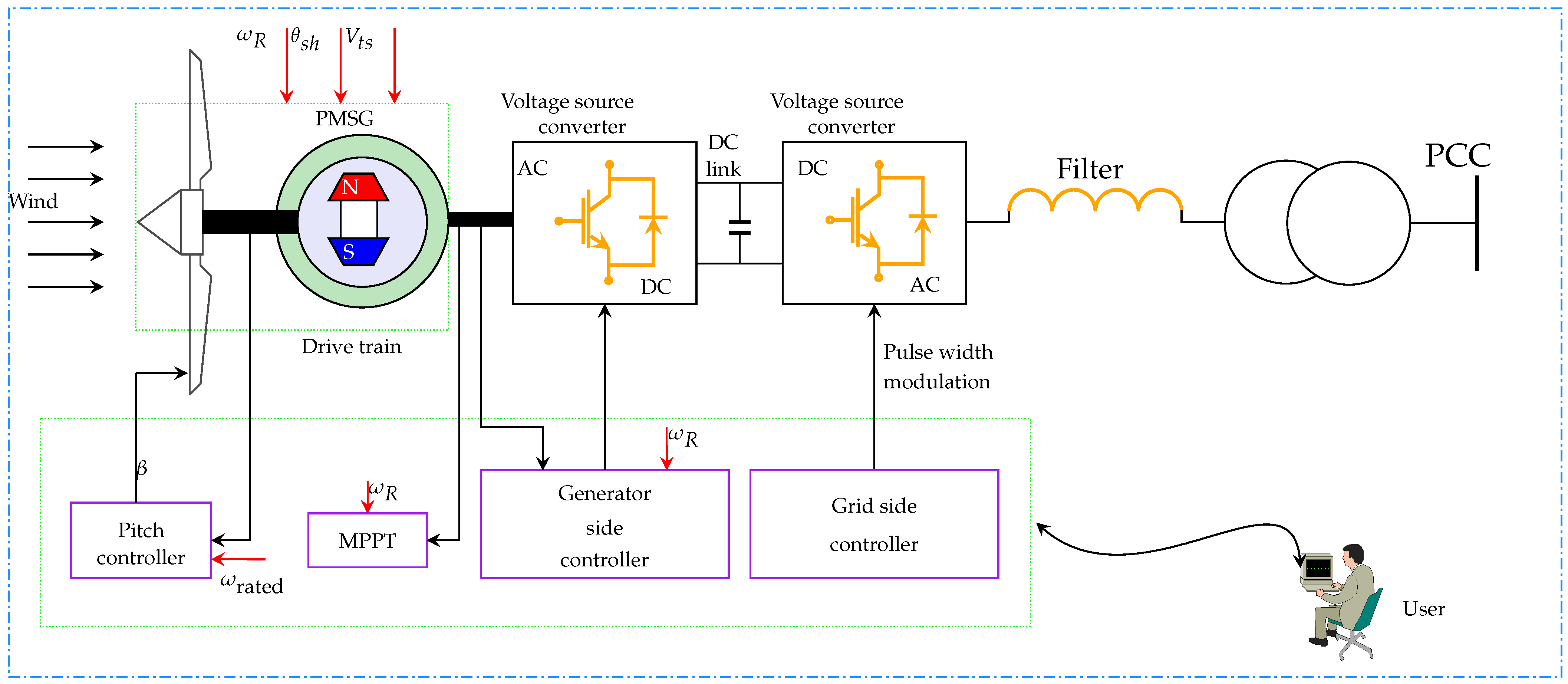
1.1. Wind Turbine Aerodynamic Model

The power coefficient C p ( λ , β ) is indicated by
C p ( λ , β ) = P T P W , P T = P W C p ( λ , β ) = 1 2 ρ π r 2 V w 3 C p ( λ , β ) ,
where P T and P W are turbine power and wind power, respectively; ρ is the air density; r is the radius of the WT blade; V w denotes the wind velocity. The tip speed ratio λ is represented by
λ = V t s × r V w = turbine   speed × radius wind   speed .
The C p ( λ , β ) is calculated as follows [2]:
C p ( λ , β ) = ( 0.44 0.0167 β ) sin π ( λ 2 ) 13 0.3 β 0.00184 ( λ 2 ) β ,
Here, β denotes the pitch angle. Researchers achieved the power coefficient C p in the range of 0.2 to 0.4 (see in [2]). According to the Betz limit, the highest power coefficient C p is 0.59. Therefore, the power coefficient C p should be kept as high as possible to generate maximum power. For variable-speed wind turbines, λ o p t =7.1, while the pitch angle β should remain at 0.

1.2. Modeling of PMSG-Based WECS

The general state–space equation of PMSG-based WECS is given below [2]:
x ˙ ( t ) = A x ( t ) + B u ( t ) + Z w ( t ) , y ( t ) = C x ( t ) ,
where A , B , Z, and C are the constant matrices; x ( t ) = [ i s d ( t ) i s q ( t ) ω R ( t ) θ s h ( t ) V t s ( t ) ] T and u ( t ) are the state vectors and control input vector, respectively, w ( t ) stands for the disturbance signal.
A = R s r L M ω R 0 0 0 ω R R s r L M ϕ L M 0 0 0 A 32 A 33 A 34 A 35 0 0 W b 0 W b 0 0 A 53 A 54 P V t s A 53 ,
B = 1 L M 1 L M 0 0 0 T ,
with        A 32 = 3 N P ϕ 8 I g , A 33 = D s W b + B W 2 I g , A 34 = K s t 2 I g , A 35 = D s W b 2 I g , A 53 = D s W b 2 I t , A 54 = K s t 2 I t ,   ω R and V t s represent the generator and turbine speed, respectively; R s r is the resistance of the stator, N P is the number of poles, ϕ denotes magnetic flux, I g is the generator inertia, I t denotes turbine inertia, W b is the base twist angle, D s denotes the damping of the shaft, and K s t is the shaft stiffness. P = [ 1 / ( 4 I t λ 3 ) ] ρ π R 5 C p ( β ) . The d and q axis machine inductances are described by L d and L q , which are both similar in nature; therefore, we assumed L d = L q = L M . Here, P clearly show that it has the product of ω R , so the designed model is nonlinear. It is more complex to use the present mathematical techniques. Thus, the nonlinear model is evaluated by applying the T-S fuzzy method. The intricate layout of a PMSG-based WECS is illustrated in Figure 1.

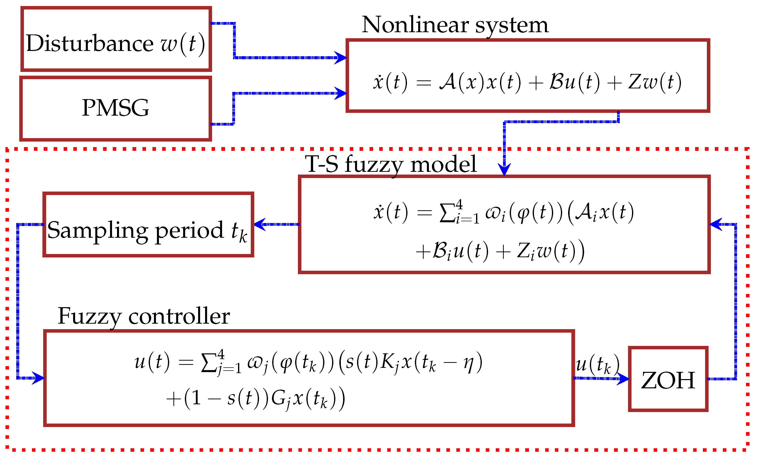
1.3. T-S Fuzzy Representation of the PMSG Model

Based on the principle of sector nonlinearity [33], the PMSG-based WECS (1) could be portrayed as a T-S fuzzy model along with a set of fuzzy IF–THEN rules:
Plant Rule i : IF ω R ( t ) is H i 1 and V t s ( t ) is H i 2 , THEN
x ˙ ( t ) = A i x ( t ) + B i u ( t ) + Z i w ( t ) , y ( t ) = C i x ( t ) , i = 1 , 2 , 3 , 4 .
Here, H i 1 and H i 2 are fuzzy sets. By implementing the T-S fuzzy rule, the nonlinear system (1) can be represented by
x ˙ ( t ) = i = 1 4 ϖ i ( φ ( t ) ) A i x ( t ) + B i u ( t ) + Z i w ( t ) , y ( t ) = i = 1 4 ϖ i ( φ ( t ) ) C i x ( t ) ,
where ϖ i ( φ ( t ) ) stands for the normalized membership function; it satisfies
ϖ i ( φ ( t ) ) = h i ( φ ( t ) ) i = 1 4 h i ( φ ( t ) ) , h i ( φ ( t ) ) = j = 1 2 H i j ( φ j ( t ) ) ,
where φ ( t ) = [ ω R V t s ] , H i j ( φ j ( t ) ) denotes the grade of membership of φ j ( t ) in H i j . It is assumed that
h i ( φ ( t ) ) 0 , i = 1 4 h i ( φ ( t ) ) > 0 t 0 .
The fuzzy system modeling conditions are assumed as
ϖ i ( φ ( t ) ) 0 , i = 1 4 ϖ i ( φ ( t ) ) = 1 .
The following is a definition of the T-S fuzzy model:
Plant Rule 1: IF ω R ( t ) is H 11 and V t s ( t ) is H 12 , THEN
A 1 = R s r L M D 1 0 0 0 D 1 R s r L M ϕ L M 0 0 0 A 32 A 33 A 34 A 35 0 0 W b 0 W b 0 0 A 53 A 54 P D 2 A 53 ,
Plant Rule 2: IF ω R ( t ) is H 11 and V t s ( t ) is H 22 , THEN
A 2 = R s r L M D 1 0 0 0 D 1 R s r L M ϕ L M 0 0 0 A 32 A 33 A 34 A 35 0 0 W b 0 W b 0 0 A 53 A 54 P D 2 A 53 ,
Plant Rule 3: IF ω R ( t ) is H 21 and V t s ( t ) is H 12 , THEN
A 3 = R s r L M D 1 0 0 0 D 1 R s r L M ϕ L M 0 0 0 A 32 A 33 A 34 A 35 0 0 W b 0 W b 0 0 A 53 A 54 P D 2 A 53 ,
Plant Rule 4: IF ω R ( t ) is H 21 and V t s ( t ) is H 22 , THEN
A 4 = R s r L M D 1 0 0 0 D 1 R s r L M ϕ L M 0 0 0 A 32 A 33 A 34 A 35 0 0 W b 0 W b 0 0 A 53 A 54 P D 2 A 53 ,
B 1 = B 2 = B 3 = B 4 = 1 / L d 1 / L d 0 0 0 ,
where ω R ( t ) [ D 1 , D 1 ] and V t s ( t ) [ D 2 , D 2 ] , D 1 and D 2 are the premise variable bounds. Then, the fuzzy membership function is defined as
H 11 ( ω R ( t ) ) = D 1 + ω R ( t ) 2 D 1 , H 12 ( V t s ( t ) ) = D 2 + V t s ( t ) 2 D 2 , H 21 ( ω R ( t ) ) = D 1 ω R ( t ) 2 D 1 , H 22 ( V t s ( t ) ) = D 2 V t s ( t ) 2 D 2 .

1.4. CMSDC Design

In this subsection, we will design a CMSDC for PMSG-based WECS. Therefore, the fuzzy CMSDC law is designed as
Control Rule j : IF ω R ( t k ) is H j 1 and V t s ( t k ) is H j 2 , THEN
u ( t ) = s ( t ) K j x ( t k η ) + ( 1 s ( t ) ) G j x ( t k ) ,
where t [ t k , t k + 1 ) , both K j and G j are the control gain matrices, η is a memory parameter, and s denotes the coupling term. x ( t k ) is the measure of x ( t ) at sampling instant t k , and that is assumed as 0 < t k + 1 t k = h k h , h > 0 , k 0 . Then, by setting h ( t ) = t t k with h ˙ ( t ) = 1 for t t k , the sampling instant t k can be represented as t k = t h ( t ) , where 0 h ( t ) h . Moreover, s ( t ) is a stochastic variable coupling both SDC and memory SDC with
s ( t ) = 1 signal forwarded , 0 if not ,
where s ( t ) obeys Bernoulli distribution white order with P r { s ( t ) = 1 } = Ξ { s ( t ) } = s and P r { s ( t ) = 0 } = 1 Ξ { s ( t ) } = 1 s . Then, the controller can be created as follows:
u ( t ) = j = 1 4 ϖ j ( φ ( t k ) ) s ( t ) K j x ( t k η ) + ( 1 s ( t ) ) G j x ( t k ) .
Substituting CMSDC (5) in the system (4), the closed-loop fuzzy PMSG-based WECS becomes
x ˙ ( t ) = i = 1 4 j = 1 4 ϖ i ( φ ( t ) ) ϖ j ( φ ( t k ) ) ( A i x ( t ) + s ( t ) B i × K j x ( t k η ) + ( 1 s ( t ) ) B i G j x ( t k ) + Z i w ( t ) ) , y ( t ) = i = 1 4 ϖ i ( φ ( t ) ) C i x ( t ) .
Further, Figure 2 illustrates the complete design of the proposed CMSDC.
Remark 1. 
This study deals with CMSDC, which is limited by Bernoulli distributed order. A stochastic variable coupling s ( t ) has been involved to coupled the SDC and MSDC. If the stochastic variable s ( t ) = 0, then the closed loop controller (5) becomes u ( t ) = j = 1 4 ϖ j ( φ ( t k ) ) G j x ( t k ) , it denotes the sampled data proportional control [2]. If s ( t ) = 1, the CMSDC (5) mitigates to u ( t ) = j = 1 4 ϖ j ( φ ( t k ) ) K j x ( t k η ) , indicating the memory SDC [34]. Thus, the PMSG-based CMSDC is more general than MSDC or SDC.
Lemma 1 
([35]). For given constant matrix R > 0 and any matrix N R 6 n × n , the below inequality holds:
t k t x ˙ T ( s ) R x ˙ ( s ) d s ( t t k ) ζ T ( t ) N R 1 N T ζ ( t ) + 2 ζ T ( t ) N t k t x ˙ ( s ) d s ,
where ζ T ( t ) = x T ( t ) x T ( t k ) and N = N 1 N 2 T .
Lemma 2 
([36]). Given the positive matrix R 2 > 0 , and continuous function x ˙ : [a,b] R n , the below inequality holds:
( b a ) a b x ˙ T ( s ) R 2 x ˙ ( s ) d s a b x ( s ) d s T R 2 a b x ( s ) d s .
Remark 2. 
If all of the local linear subsystems have the same disturbance attenuation index, (i.e., χ = 1 , the classical H performance ( 0 y T ( t ) y ( t ) d t γ 2 0 w T ( t ) w ( t ) d t )   ) , the end outcome of the design will be the same as in [37]. Most studies investigate fuzzy systems with disturbances using a conventional H performance index. For example, the researchers used many control methods such as sliding-mode control [31] and sampled-data control [38] to study the conventional infinity performance index for TS fuzzy systems with disturbance. This study proposed the MFD H performance index for T-S fuzzy PMSG-based WECS through fuzzy CMSDC, in contrast to earlier research.
Problem 1. 
The PMSG-based WECS is said to be asymptotically stable with MFD H performance disturbance attenuation level bound γ ^ if the solution of the states for the system satisfies the following condition:
  • In the absence of w ( t ) , the closed-loop system (6) is asymptotically stable.
  • Given the predefined constant γ ^ > 0 and under the zero initial condition, throughout other than zero w ( t ) L 2 [ 0 , ) , the closed-loop system (6) fulfills the following inequality:
0 y T ( t ) y ( t ) d t γ ^ 2 0 w T ( t ) w ( t ) d t ,
where γ ^ = χ ϖ 1 ( φ ( t ) ) + i = 2 4 ϖ i ( φ ( t ) ) γ with 0 < χ 1 .

2. Main Results

The stability and stabilization of the PMSG-based WECS are derived based on the LMI approach and the LKF technique in the following subdivisions.

2.1. Stability of PMSG

In this subsection, the proposed adequate circumstances are summed in the following Theorem for the closed-loop system (6), which is a solution to Problem 1.
Theorem 1. 
Given positive scalars η, α, β, γ ^ and upper bound h, h k ( 0 , h ] , the system (6) is asymptotically stable with the H performance, if there exist the matrices G > 0 , M 1 > 0 , M 4 > 0 , M 6 > 0 , K > 0 , O > 0 , P > 0 , symmetric matrices I , N , and any appropriate dimensional matrices, L 1 , L 2 ,   M b ( b = 2 , 3 , 5 ) and T l ( l = 1 , 2 , 3 , 4 , 5 ) , such that the following inequalities hold:
Ω i j + h k Ψ < 0 ,
Ω i j + h k Π h k T M 1 < 0 ,
where
Ω i j = e 1 T { K + 2 T 1 N O P } e 1 + e 2 T { 2 M 2 2 T 2 N O } e 2 e 3 T { π 2 4 I } e 3 e 4 T { π 2 4 I + K } e 4 + e 5 T { h 2 I + η 2 K } e 5 + S y m [ e 1 T { M 2 T 1 + T 2 T + N + O } e 2 + e 1 T K e 3 e 1 T M 3 e 4 + e 1 T G e 5 + e 2 T M 3 e 4 + e 3 T π 2 4 I e 4 + ( e 1 T L 1 + e 5 T L 2 ) × ( e 5 + A i e 1 + s ( t ) B i K j e 4 + ( 1 s ( t ) ) B i G j e 2 + Z i e 6 ) ] + e 1 T C i T C i e 1 Υ i e 6 T e 6 , Ψ = e 2 T M 4 e 2 + e 4 T M 6 e 4 + e 5 T M 1 e 5 + S y m [ e 1 T { N T + O T + P } e 5 + e 2 T M 5 e 4 + e 2 T { M 2 T N T O T } e 5 + e 4 T M 3 T e 5 ] , Π = e 2 T M 1 e 2 e 2 T M 5 e 4 e 4 T M 6 e 4 , Υ 1 = χ γ 2 , Υ i = γ 2 ( i = 2 , 3 , 4 ) , T = T 1 T T 2 T T 3 T T 4 T T 5 T 0 T e b = [ 0 5 × ( b 1 ) 5 , I 5 , 0 5 × ( 6 b ) 5 ] , ( b = 1 , 2 , 3 , , 6 ) .
Proof. 
Consider the following LKF for PMSG-based
WECS:
V ( t ) = x T ( t ) G x ( t ) + d = 1 4 V d ( t ) ,
where
V 1 ( t ) = ( h k h ( t ) ) t k t x ˙ ( s ) x ( t k ) x ( t k η ) T M x ˙ ( s ) x ( t k ) x ( t k η ) d s , V 2 ( t ) = h 2 t k η t x ˙ T ( s ) I x ˙ ( s ) d s π 2 4 t k η t η [ x ( s ) x ( t k η ) ] T I [ x ( s ) x ( t k η ) ] d s , V 3 ( t ) = η η 0 t + θ t x ˙ T ( s ) K x ˙ ( s ) d s d θ + ( h k h ( t ) ) ( x ( t ) x ( t k ) ) T N ( x ( t ) x ( t k ) , V 4 ( t ) = ( h k h ( t ) ) t k t x ˙ ( s ) d s T O t k t x ˙ ( s ) d s + ( h k h ( t ) ) x T ( t ) P x ( t ) ,
in which
M = M 1 M 2 M 3 M 4 M 5 M 6 .
Calculate the weak infinitesimal operator of L V ( t ) ; we have
L V ( t ) = 2 x T ( t ) G x ˙ ( t ) + d = 1 4 L V d ( t ) ,
where
L V 1 ( t ) = t k t x ˙ ( s ) x ( t k ) x ( t k η ) T M 1 M 2 M 3 M 4 M 5 M 6 x ˙ ( s ) x ( t k ) x ( t k η ) d s + h k h ( t ) x ˙ ( t ) x ( t k ) x ( t k η ) T M 1 M 2 M 3 M 4 M 5 M 6 x ˙ ( t ) x ( t k ) x ( t k η ) , L V 2 ( t ) = h 2 [ x ˙ T ( t ) I x ˙ ( t ) ] π 2 4 [ x ( t η ) x ( t k η ) ] T I [ x ( t η ) x ( t k η ) ] , L V 3 ( t ) = η 2 x ˙ ( t ) K x ˙ ( t ) x ( t ) x ( t η ) T K x ( t ) x ( t η ) x ( t ) x ( t k ) T N × x ( t ) x ( t k ) + ( h k h ( t ) ) S y m { x ˙ T ( t ) N ( x ( t ) x ( t k ) ) } , L V 4 ( t ) = x ( t ) x ( t k ) T O x ( t ) x ( t k ) + 2 ( h k h ( t ) ) × x ˙ ( t ) O x ( t ) x ( t k x T ( t ) P x ( t ) + 2 ( h k h ( t ) ) × x T ( t ) P x ˙ ( t ) .
By using the Lemma 1 in L V 1 ( t ) , the following inequality holds with M 1  ≥ 0 and any matrix T :
t k t x ˙ T ( s ) M 1 x ˙ ( s ) d s ( t t k ) ξ T ( t ) T M 1 1 T T ξ ( t ) + 2 ξ T ( t ) T [ x ( t ) x ( t k ) ] ,
and Lemma 2 Jensen’s inequality [36] in L V 3 ( t ) , the following inequality holds with K 0 :
η t η t x ˙ T ( s ) K x ˙ ( s ) d s t η t x ( s ) d s T K t η t x ( s ) d s ,
where ξ T ( t ) = x T ( t ) x T ( t k ) x T ( t η ) x T ( t k η ) x ˙ T ( t ) ω T ( t ) . Additionally, for any matrices L 1 and L 2 , the zero equation holds as,
E { 0 = 2 { x T ( t ) L 1 + x ˙ T ( t ) L 2 } { i = 1 4 j = 1 4 ϖ i ( φ ( t ) ) ϖ j ( φ ( t k ) ) × ( A i x ( t ) + s ( t ) B i K j x ( t k η ) + ( 1 s ( t ) ) B i G j x ( t k ) + Z i w ( t ) x ˙ ( t ) ) } } .
From (14), (15) and adding (16) with (13), then
E { L V ( t ) + y T ( t ) y ( t ) γ ^ 2 w T ( t ) w ( t ) } i = 1 4 j = 1 4 ϖ i ( φ ( t ) ) ϖ j ( φ ( t k ) ) ξ T ( t ) [ Ω i j + ( h k h ( t ) ) Ψ + ( t t k ) × ( Π + T M 1 1 T T ) ] ξ ( t ) .
It must be noted that (17) is a blend of ( t t k ) as well as ( h k h ( t ) ) over h k ( 0 , h ] . From (10) and (11), we can say that E { L V ( t ) } < 0 . Thus, the PMSG-based WECS (6) is asymptotically stable with the fuzzy CMSDC scheme. This completes the source of the theorem.    □

2.2. Stabilization of PMSG

In this section, the stabilization state is summed in the pursuing Theorem 2:
Theorem 2. 
Given positive scalars η , α , β , γ ^ and upper bound h , h k ( 0 , h ] , the closed-loop system (6) is asymptotically stable; if one can obtain the matrices G ¯ > 0 , M ¯ 1 > 0   M ¯ 4 > 0 , M ¯ 6 > 0 , K ¯ > 0 , O ¯ > 0 , P ¯ > 0 , and symmetric matrices I ¯ , N ¯ , as well as any appropriate dimensional matrices L,  M b ¯   ( b = 2 , 3 , 5 ) and T l ¯   ( l = 1 , 2 , 3 , 4 , 5 ) , then the following LMIs hold:
Ω ¯ i j + h k Ψ ¯ C ^ i I < 0 ,
Ω ¯ i j + h k Π ¯ h k T ¯ C ^ i M 1 ¯ 0 I < 0 .
where
Ω ¯ i j = e 1 T { K ¯ + 2 T ¯ 1 N ¯ O ¯ P ¯ } e 1 + e 2 T { 2 M ¯ 2 2 T ¯ 2 N ¯ O ¯ } e 2 e 3 T { π 2 4 I ¯ } e 3 e 4 T { π 2 4 I ¯ + K ¯ } e 4 + e 5 T { h 2 I ¯ + η 2 K ¯ } e 5 + S y m [ e 1 T { M ¯ 2 T ¯ 1 + T ¯ 2 T + N ¯ + O ¯ } e 1 + e 1 T K ¯ e 3 e 1 T M ¯ 3 e 4 + e 1 T G ¯ e 5 + e 2 T M ¯ 3 e 4 + e 3 T π 2 4 I ¯ e 4 + ( e 1 T α + e 5 T β ) × ( L e 5 + A i L e 1 + s ( t ) B i X j e 4 + ( 1 s ( t ) ) B i Y j e 2 + Z i e 6 ) ] Υ i e 6 T e 6 , Ψ ¯ = e 2 T M ¯ 4 e 2 + e 4 T M ¯ 6 e 4 + e 5 T M ¯ 1 e 5 + S y m [ e 1 T { N ¯ T + O ¯ T + P ¯ } e 5 + e 2 T M ¯ 5 e 4 + e 2 T { M ¯ 2 T N ¯ T O ¯ T } e 5 + e 4 T M ¯ 3 T e 5 ] , Π ¯ = e 2 T M ¯ 1 e 2 e 2 T M ¯ 5 e 4 e 4 T M ¯ 6 e 4 , Υ 1 = χ γ 2 , Υ i = γ 2 ( i = 2 , 3 , 4 ) , C ^ i = c o l u m L T C ¯ i T 0 0 0 0 0 .
Here, we can calculate the control gain matrices K j and G j through K j = X j L 1 and G j = Y j L 1 , respectively.
Proof. 
Define L 1 = α L T , L 2 = β L T , L T G L = G ¯ , L T I L = I ¯ , L T K L = K ¯ , L T N L = N ¯ , L T O L = O ¯ , L T P L = P ¯ , L T M r L = M ¯ r ( r = 1 , 2 , 3 , 4 , 5 , 6 ) . Then, the LMIs (10) and (11) are pre-multiplied and post-multiplied on both sides with d i a g { L T , L T , L T , L T , L T , I } and its transpose, respectively. Then, applying the Schur complement, one can obtain the LMIs (18) and (19). Therefore, the PMSG-based WECS system (6) is asymptotically stable, holding the H disturbance attenuation level of γ ^ . The entire proof is complete.    □
Remark 3. 
In addition, FMFs between the control and system are not synchronous due to the digital transmission condition ω i ( ϕ ( t ) ) ω i ( ϕ ( t k ) ) . Thus, we consider the error information of FMFs condition | ω i ( ϕ ( t ) ) ω i ( ϕ ( t k ) ) | τ i , in Theorem 2, and we can obtain a more accurate result based on the Lemma 1 in [39] the following corollary.
Corollary 1. 
Let | ω i ( ϕ ( t ) ) ω i ( ϕ ( t k ) ) | τ i , for given positive scalars η , α , β , γ ^ and upper bound h , h k ( 0 , h ] ; the closed-loop system (6) is asymptotically stable. If one can obtain the matrices G ¯ > 0 , M ¯ 1 > 0   M ¯ 4 > 0 , M ¯ 6 > 0 , K ¯ > 0 , O ¯ > 0 , P ¯ > 0 , symmetric matrices I ¯ , N ¯ , and any appropriate dimensional matrices L, M b ¯   ( b = 2 , 3 , 5 ) ,   T l ¯   ( l = 1 , 2 , 3 , 4 , 5 )   T 1 i j = T 1 j i T ,   ( i , j = 1 , 2 , 3 , 4 ) , then the following LMIs hold:
Y s i j + Y s j i T T s i j + T s j i T ,
Ω s i j 2 Y s i j + r = 1 p ( Y s i r + Y s r i T ) T s i ( j + p ) + T s ( j + p ) i T ,
S s 11 S s 12 S s 11 < 0 ,
where Y s i j = H s i j L s i j ,   Y s i j = H s i j L s i j , ( s = 1 , 2 )
S s 11 = T s 11 T s 1 p T s 1 p T s p p , S s 12 = T s 1 ( p + 1 ) T s 1 ( 2 p ) T s 1 ( p + 1 ) T s 4 ( 2 p ) , Ω 1 i j = Ω ¯ i j + h k Ψ ¯ C ^ i I , Ω 2 i j = Ω ¯ i j + h k Π ¯ h k T ¯ C ^ i M 1 ¯ 0 I ,
the terms of Ω s i j   ( s = 1 , 2 ) are given in Theorem 2. Furthermore, we can calculate the control gain matrices K j and G j through K j = X j L 1 and G j = Y j L 1 , respectively.
Proof. 
The proof of this corollary directly follows from Theorem 2 and Lemma 1 in [39]; therefore, the detailed proof is omitted.    □
Remark 4. 
Recently, there has been growing interest among researchers in the use of mismatched membership functions for industrial applications, aimed at reducing conservatism in stability conditions. For instance, in [40,41], authors have explored stability analysis using mismatched functions, where the membership function in the controller differs from that of the plant process. Their findings indicate less conservative stability conditions compared to traditional approaches. Consequently, Corollary 1 establishes stabilization criteria under mismatched membership functions using Lemma 1 in [39].
Remark 5. 
We derived the stability and stabilization conditions of T-S fuzzy system (6) with H attenuation level γ ^ as shown in Theorems 1 and 2. We assume that w ( t ) = 0 and obtain the following system:
x ˙ ( t ) = i = 1 4 j = 1 4 ϖ i ( φ ( t ) ) ϖ j ( φ ( t k ) ) ( A i x ( t ) + s ( t ) B i K j x ( t k η ) + ( 1 s ( t ) ) B i G j x ( t k ) ) ,
and for any matrix L 1 and L 2 , the following zero equation is true:
E { 0 = 2 { x T ( t ) L 1 + x ˙ ( t ) L 2 } i = 1 4 j = 1 4 × ϖ i ( φ ( t ) ) ϖ j ( φ ( t k ) ) × { A i x ( t ) + s ( t ) B i K j × x ( t k η ) + ( 1 s ( t ) ) B i G j x ( t k ) x ˙ ( t ) } } .
From Theorem 1, can be gathered the LKF as well as its derivatives. That is summed in the resulting Corollary 2.
Corollary 2. 
The provided positive scalars η , α , β and upper bound h , h k ( 0 , h ] ; if one can obtain the matrices G > 0 , M 1 > 0 , M 4 > 0 , M 6 > 0 , K > 0 , O > 0 , P > 0 , symmetric matrices I , N , and an appropriate dimensions matrices of L 1 , L 2 ,   M b ( b = 2 , 3 , 5 ) and T l ( l = 1 , 2 , 3 , 4 , 5 ) , then following LMIs hold:
Ω i j + h k Ψ < 0 Ω i j + h k Π h k T M 1 < 0
where
Ω i j = e 1 T { K + 2 T 1 N O P } e 1 + e 2 T { 2 M 2 2 T 2 N O } e 2 e 3 T { π 2 4 I } e 3 e 4 T { π 2 4 I + K } e 4 + e 5 T { h 2 I + η 2 K } e 5 + S y m [ e 1 T { M 2 T 1 + T 2 T + N + O } e 1 + e 1 T K e 3 e 1 T M 3 e 4 + e 1 T G e 5 + e 2 T M 3 e 4 + e 3 T π 2 4 I e 4 + ( e 1 T L 1 + e 5 T L 2 ) × ( e 5 + A i e 1 + s ( t ) B i K j e 4 + ( 1 s ( t ) ) B i G j e 2 ) ] Ψ = e 2 T M 4 e 2 + e 4 T M 6 e 4 + e 5 T M 1 e 5 + S y m [ e 1 T { N T + O T + P } e 5 + e 2 T M 5 e 4 + e 2 T { M 2 T N T O T } e 5 + e 4 T M 3 T e 5 ] , Π = e 2 T M 1 e 2 e 2 T M 5 e 4 e 4 T M 6 e 4 , e b = [ 0 5 × ( b 1 ) 5 , I 5 , 0 5 × ( 6 b ) 5 ] , ( b = 1 , 2 , 3 , , 6 ) .
Then, the system (6) is globally asymptotically stable. Furthermore, we can calculate the control gain matrices K j and G j through K j = X j L 1 and G j = Y j L 1 , respectively.
Proof. 
The proof of the corollary is instantly received from Theorem 1. Therefore, the proof is completed.    □

3. Numerical Validation

We divided this section into three parts to validate the proposed method’s efficacy and applicability. In the first part, the PMSG model (6) is utilized as a design example. Moreover, the same model is evaluated using various memory parameters η and pitch angles β . In the second part, evaluate the MFD H performance index. Finally, as a comparison example, Rossler’s system is examined and resolved to prove the efficiency and superiority of the proposed approach. The Matlab LMI control toolbox is used to solve the complete dynamical model of the PMSG-based WECS.

3.1. Design Example

In this design example, we numerically evaluate the PMSG-based WECS, including the acceptable derived condition as in Theorem 2, which proves the asymptotic stability of the PMSG-based WECS. The parameters of PMSG-based WECS are given in Table 1, which is referred from [2]. The defined scalars are determined as α = 0.005, β = 0.007 η = 0.02, s = 0.7, and γ = 0.3. Moreover, we assume C 1 = C 2 = C 3 = C 4 = [ 1 0 0 0 0 ]. In addition, the disturbance matrix Z i is considered as the same input matrix B i , i.e., Z i = B i . For solving the LMI condition based on Algorithm 1, the required control gain matrices are calculated as follows:
K j = [ 0.3755 0.6057 0.1964 0.1619 0.0017 ] , G j = [ 3.7118 1.5248 0.2043 0.0574 0.8291 ] ,
where i and j = { 1 , 2 , 3 , 4 } .
Algorithm 1 Calculating the control gain matrices and maximum allowable upper bound (MAUB) of h k .
  • Given system matrices A i , B i , C i ( i = 1 , 2 , 3 , 4 . ), scalars η , α , β , γ ^ , h-upper bound and μ is a step increment of h.
  • Set h = h + μ , by utilizing the f e a s p solver in the MATLAB LMI toolbox, solve the LMIs (18) and (19) with there existing matrices G ¯ > 0 , M ¯ 1 > 0   M ¯ 4 > 0 , M ¯ 6 > 0 , K ¯ > 0 , O ¯ > 0 , P ¯ > 0 , symmetric matrices I ¯ , N ¯ , and any appropriate dimensional matrix L, M b ¯   ( b = 2 , 3 , 5 ) and T l ¯   ( l = 1 , 2 , 3 , 4 , 5 ) in Theorem 2. Furthermore, reduce the H performance index γ ^ with the tuning parameter χ , 0 < χ 1 .
  • If there is a feasible LMIs (18) and (19) and the matrices X j , Y j and L in step 2, go to step 2; otherwise, set h = h μ .
  • Calculate the control gain matrices K j = X j L 1 and G j = Y j L 1 and MAUB of delay h.
As illustrated in Figure 3, one can observe that the states i s d , i s q , ω R , θ s h and V t s are stabilized under the proposed CMSDC. Furthermore, Figure 4 demonstrated the control responses of u ( t ) .

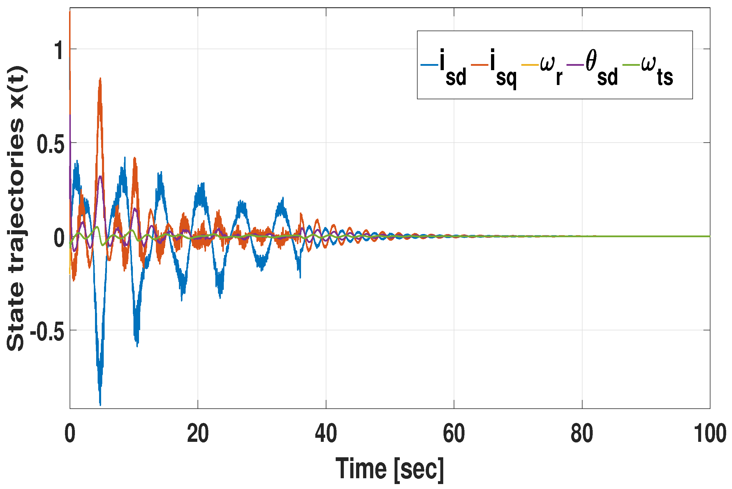
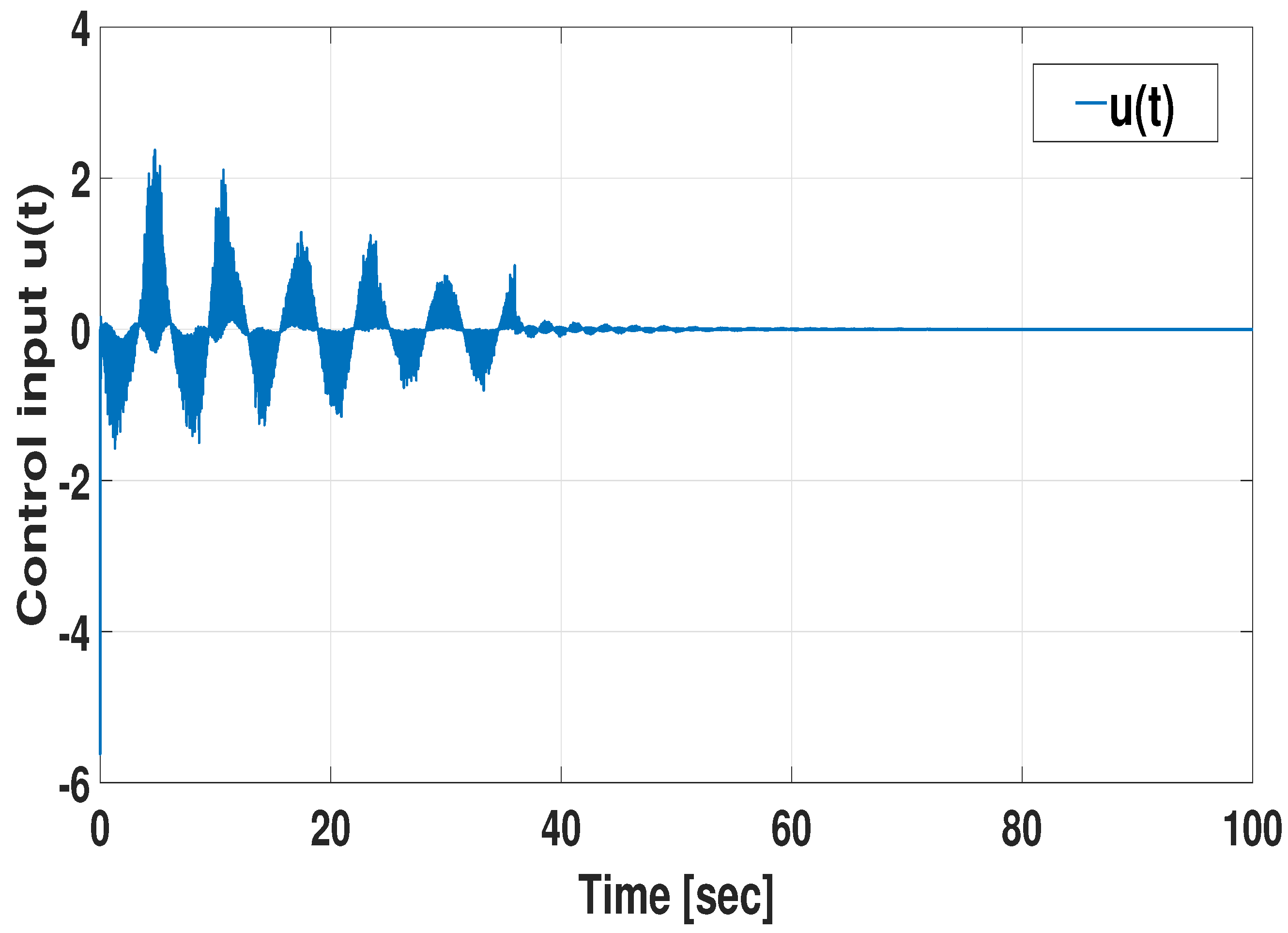
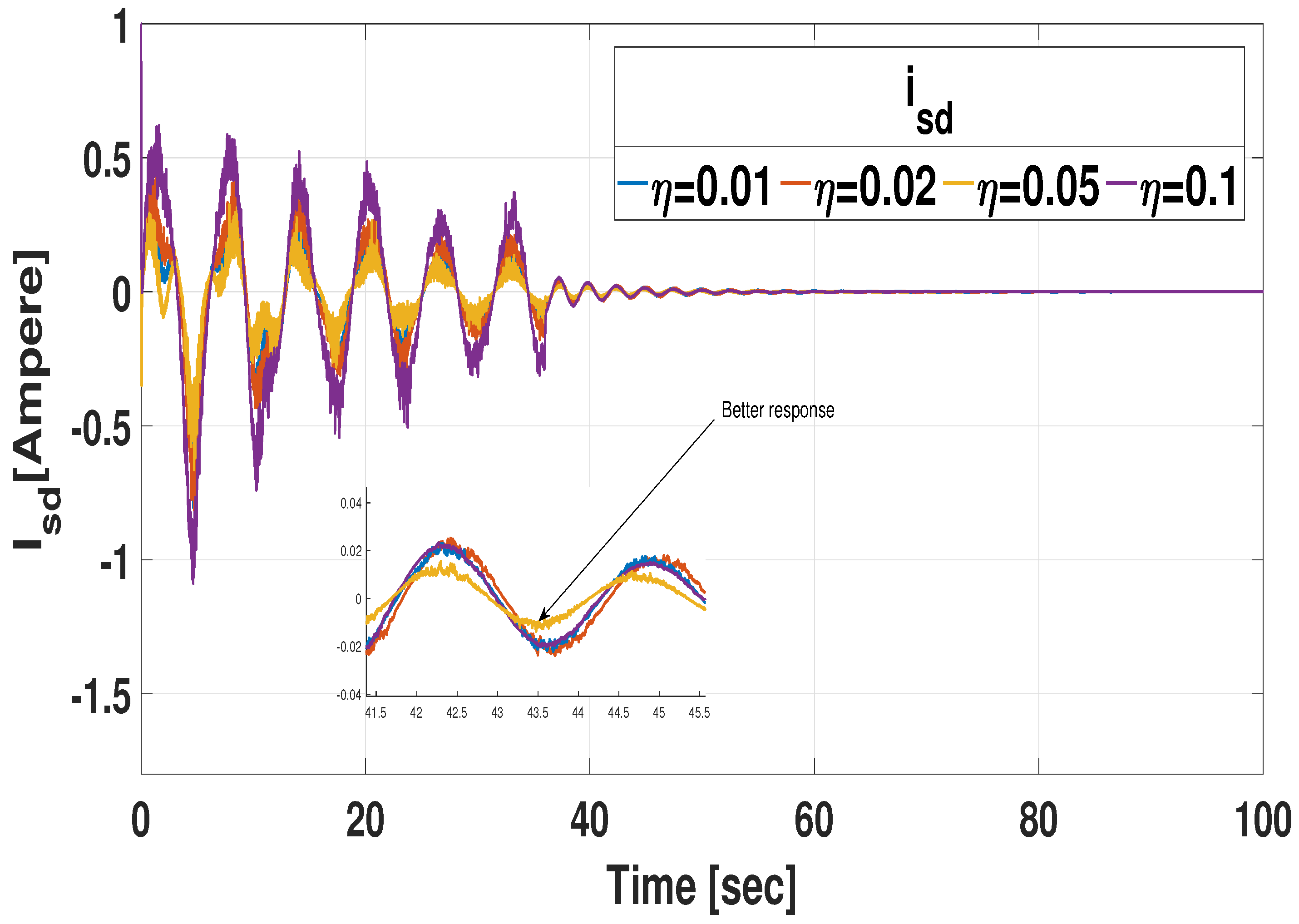
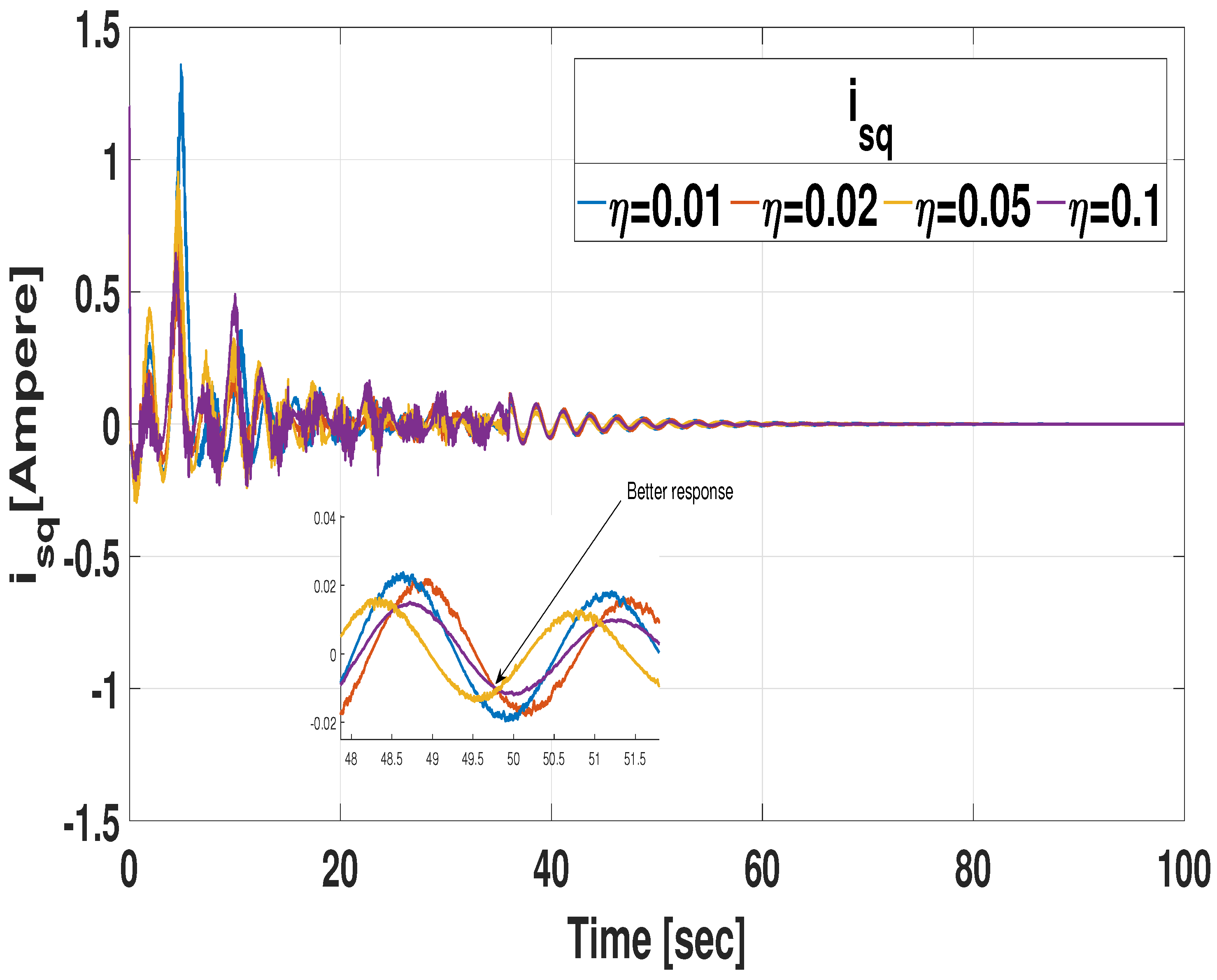
3.1.1. Simulation with Respect to Various Memory Parameter

This subsection shows the effectiveness of the memory parameter η in the proposed CMSDC. For simulation purposes, we fixed the pitch angle as β = 0 . 5 . Then, the memory parameter η is changed to 0.01, 0.02, 0.05, and 0.1. Moreover, using Theorem 2, the corresponding gain matrices are mentioned in Table 2 with different memory parameters. Based on the calculated gain matrices, the dynamical behavior of PMSG-based WECS while changing the η value is plotted in Figure 5 and Figure 6, respectively. These figures ensure i s d and i s q currents behaviors changing according to memory parameter η . In addition, the better performance is mentioned in graphs itself.

3.1.2. Simulation Concerning Pitch Angles
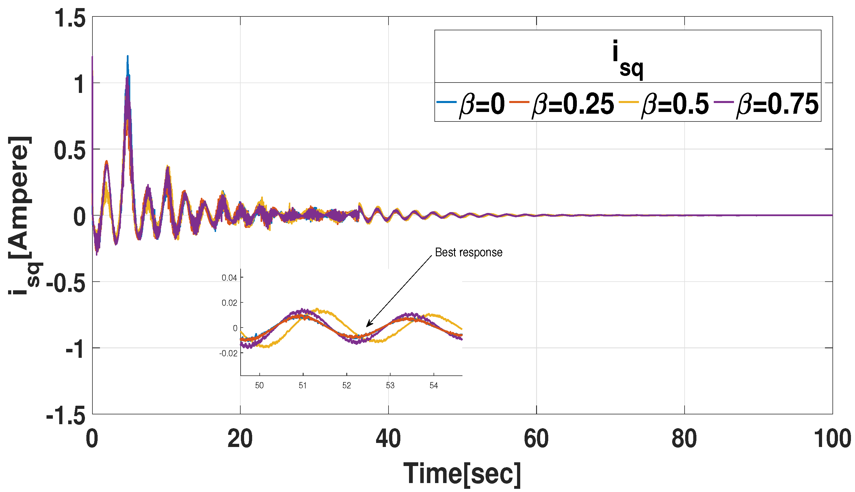
This subsection evaluates the function of β in the PMSG-based WECS. The parameters of the PMSG-based WECS are used in the same way as in the above subsection. In addition, consider the various pitch angles β as 0 , 0 . 25 , 0 . 5 , and 0 . 75 . Then the i s d and i s q currents controlled behavior of the PMSG-based WECS model is depicted to investigate the dynamic aspects with different pitch angles for the fixed-membership boundary.
By utilizing the various pitch angles, we acquire the power coefficient and their gain matrices, which are tabulated in Table 3. Furthermore, the behavior of i s d and i s q currents are displayed in Figure 7 and Figure 8, respectively. It demonstrates that changing the pitch angle has a significant impact on the performance of a PMSG-based WECS. As displayed in Figure 7 and Figure 8, we confirm that, when utilizing the proposed controller, the considered PMSG-based WECS is fruitfully controlled and reaches the global asymptotic stability in the presence of disturbance.

3.2. Evaluation of the MFD H Performance Index

This subsection deals with the numerical evaluation of the MFD H performance index by using various χ values ( 0 < χ 1 ). In this respect, the MFD H performance index is derived with various χ values by using the above-mentioned system characteristics and Theorem 2. The calculated H bound values are presented in Table 4. Moreover, for a better understanding of the H-infinity bound computation technique, one particular example is taken and presented here.
γ ^ = ( 0.5 × ϖ 1 ( φ ( t ) ) + ν ) × 0.36 [ 0.4677 , 0.6 ] .
where ν = ϖ 2 ( φ ( t ) ) + ϖ 3 ( φ ( t ) ) + ϖ 4 ( φ ( t ) ) . Moreover, from (9), the proposed fuzzy MFD H technique becomes a traditional H method when the χ is set to 1. By using the conventional H approach and Theorem 2, and setting the γ = 0.4 , we can acquire the performance index of 0.4. At the same time, the proposed MFD approach achieved a small performance index, i.e., γ ^ m i n = 0.3521 . As a result, when compared to the traditional technique, the suggested approach provides a superior performance index. In this respect, several tests have been carried out depending on the different tuning parameters c h i , and the determined H bound behaviors are shown in Figure 9. It is absolutely clear that the proposed MFD H approach accurately eliminates the disturbance compared to the conventional H method and assures the suggested method’s superiority.

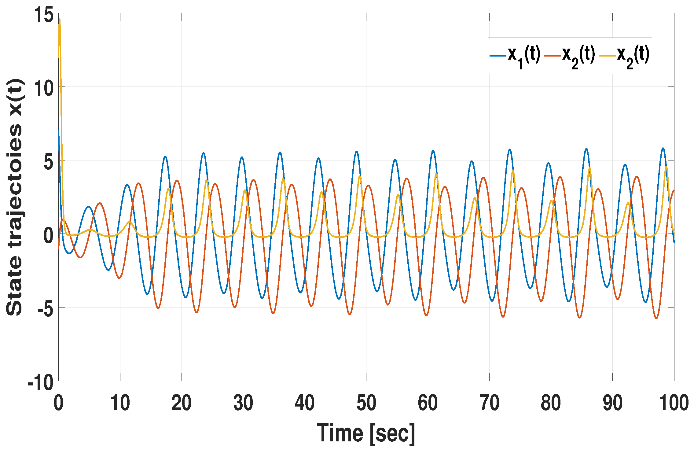
3.3. Comparative Example (Effectiveness of CMSDC Scheme)

In this subsection, Rossler’s system [30] is examined and resolved to prove the efficiency and superiority of the designed CMSDC. Rossler’s system dynamics, including input terms, are represented by
x ˙ 1 ( t ) = x 2 ( t ) x 3 ( t ) , x ˙ 2 ( t ) = x 1 ( t ) + a ¯ x 2 ( t ) , x ˙ 3 ( t ) = b ¯ x 1 ( t ) ( c ¯ x 1 ( t ) x 3 ( t ) + u ( t ) ) ,
where x 1 ( t ) , x 2 ( t ) and x 3 ( t ) , denote as state variables, a ¯ , b ¯ and c ¯ are constants. u ( t ) denotes control input. The Rossler’s system with x 1 ( t ) [ c ¯ d , c ¯ + d ] can have described by the T-S fuzzy system with
A 1 = 0 1 1 1 a ¯ 0 b ¯ 0 d , A 2 = 0 1 1 1 a ¯ 0 b ¯ 0 d , B 1 = B 2 = 0 0 1 ,
the membership functions are ϖ 1 ( x 1 ( t ) ) = c ¯ + d x 1 ( t ) 2 d and ϖ 2 ( x 1 ( t ) ) = 1 ϖ 1 ( x 1 ( t ) ) .
In such a case, we take a ¯ = 0.3 ,   b ¯ = 0.5 ,   c ¯ = 5 and d = 10 . By choosing α = 0.05, β = 0.8, s = 0.5, and η = 0.01, the proposed sufficient requirement in Corollary 2 is validated and we achieved largest sampling interval h = 0.1532 . In addition, the largest upper bound of the sampling interval is derived to be 0.1681 based on Corollary 1.
The time responses of the solution trajectories x 1 ( t ) , x 2 ( t ) and x 3 ( t ) of (27) without control inputs are shown in Figure 10. The state trajectories of system (27) with control inputs are shown in Figure 11, demonstrating that state trajectories are convergent to origin under the proposed control method. Aside from that, Figure 12 shows the response of control input. Furthermore, the obtained maximum sampling interval is compared with existing methods [30,42,43,44], which is given in Table 5. Finally, based on the findings in Table 5, we can conclude that the proposed CMSDC (5) is capable of obtaining a less conservative outcome than existing works [30,42,43,44] with relation to the maximum upper limit.

4. Conclusions

This study has described the stability and stabilization problem for surface-mounted PMSG-based WECS via the CMSDC approach, limited by a Bernoulli distribution order. The superiority of this study is to design a CMSDC with constant signal transmission delay while acting disturbance in the system. Moreover, the MFD H -based CMSDC has been proposed, which successfully attenuated the system disturbance. Furthermore, by utilizing LKF and integral inequality, sufficient requirements have been derived in the form of LMIs, which ensured that the PMSG-based WECS is globally asymptotically stable under the CMSDC. Finally, from the numerical example, we demonstrated the proposed controller’s effectiveness with reduced conservativeness and the derived results. In [45], the authors examined a neural-event-triggered control approach combined with an adaptive critic learning strategy for nonlinear wind turbine systems. Moreover, the authors of [46] investigated event-triggered H blood glucose regulation issues for type 1 diabetes using a networked artificial pancreas. Furthermore, researchers have explored an event-triggered control approach combined with fractional stochastic neural networks in [47]. Inspired by the above-mentioned literature [45,46,47], this study model will be enlarged and explored for disturbances caused by wind speed and also consider large-scale wind farms with an event-triggered mechanism in future work. In addition, the proposed control mechanism for PMVG-based WECS under actuator fault will be studied as another future direction.

Author Contributions

Conceptualization, A.A.Y.; Methodology, A.A.Y.; Validation, A.A.Y. and S.R.L.; Investigation, A.A.Y., S.R.L., N.G. and J.H.J.; Writing—original draft, A.A.Y.; Writing—review and editing, A.A.Y., S.R.L., J.H.J., N.G. and Y.H.J.; Visualization, A.A.Y.; Supervision, S.R.L., J.H.J. and Y.H.J.; Funding acquisition, Y.H.J. All authors have read and agreed to the published version of the manuscript.

Funding

This work was supported in part by the Basic Science Research Program under Grant NRF-2016R1A6A1A03013567 and Grant NRF-2021R1A2B5B01001484 and by the framework of the International Cooperation Program under Grant NRF-2022K2A9A2A06045121 through the National Research Foundation of Korea (NRF) funded by the Ministry of Education, Republic of Korea.

Data Availability Statement

Data sharing is not applicable to this article as no datasets were generated or analyzed during the current study.

Conflicts of Interest

The authors have no relevant financial or non-financial interests to disclose. The authors declare that they have no conflicts of interest.

References

  1. Gu, Y.; Huang, Y.; Wu, Q.; Li, C.; Zhao, H.; Zhan, Y. Isolation and protection of the motor-generator pair system for fault ride-through of renewable energy generation systems. IEEE Access 2020, 8, 13251–13258. [Google Scholar] [CrossRef]
  2. Mani, P.; Lee, J.H.; Kang, K.W.; Joo, Y.H. Digital controller design via LMIs for direct-driven surface mounted PMSG-based wind energy conversion system. IEEE Trans. Cybern. 2020, 50, 3056–3067. [Google Scholar] [CrossRef] [PubMed]
  3. Ghabraei, S.; Moradi, H.; Vossoughi, G. Investigation of the effect of the added mass fluctuation and lateral vibration absorbers on the vertical nonlinear vibrations of the offshore wind turbine. Nonlinear Dyn. 2021, 103, 1499–1515. [Google Scholar] [CrossRef]
  4. Mayilsamy, G.; Lee, S.R.; Joo, Y.H. An improved model predictive control of back-to-back three-level NPC converters with virtual space vectors for high power PMSG-based wind energy conversion systems. ISA Trans. 2023, 143, 503–524. [Google Scholar] [CrossRef] [PubMed]
  5. Apata, O.; Oyedokun, D.T.O. Novel reactive power compensation technique for fixed speed wind turbine generators. In Proceedings of the IEEE PES/IAS Power Africa, Cape Town, South Africa, 28–29 June 2018; pp. 628–633. [Google Scholar]
  6. Soufi, Y.; Kahla, S.; Bechouat, M. Particle swarm optimization based sliding mode control of variable speed wind energy conversion system. Int. J. Hydrogen Energy 2016, 41, 20956–20963. [Google Scholar] [CrossRef]
  7. Mousa, H.H.; Youssef, A.R.; Mohamed, E.E. Optimal power extraction control schemes for five-phase PMSG based wind generation systems. Eng. Sci. Technol. Int. J. 2020, 23, 144–155. [Google Scholar] [CrossRef]
  8. Marques, J.; Pinheiro, H.; Gründling, H.A.; Pinheiro, J.R.; Hey, H.L. A survey on variable-speed wind turbine system. Network 2003, 24, 26. [Google Scholar]
  9. Hou, L.; Wang, B.; Zhu, B. Energy extraction characteristic of the flapping wing type vertical axis turbine. IET Renew. Power Gener. 2020, 14, 2604–2611. [Google Scholar] [CrossRef]
  10. Bharathi, S.L.K.; Selvaperumal, S. MGWO-PI controller for enhanced power flow compensation using unified power quality conditioner in wind turbine squirrel cage induction generator. Microprocess. Microsystems 2020, 76, 103080. [Google Scholar] [CrossRef]
  11. Venkateswaran, R.; Joo, Y.H. Retarded sampled data control design for interconnected power system with DFIG-based wind farm: LMI approach. IEEE Trans. Cybern. 2022, 52, 5767–5777. [Google Scholar] [CrossRef]
  12. Mayilsamy, G.; Lee, S.R.; Joo, Y.H. Open-switch fault diagnosis in back-to-back NPC converters of PMSG-based WTS via zero range value of phase currents. IEEE Trans. Power Electron. 2023, 39, 4687–4703. [Google Scholar] [CrossRef]
  13. Jiao, N.; Liu, W.; Meng, T.; Sun, C.; Jiang, Y. Decoupling start control method for aircraft wound-rotor synchronous starter-generator based on main field current estimation. IET Electr. Power Appl. 2018, 13, 863–870. [Google Scholar] [CrossRef]
  14. Errami, Y.; Ouassaid, M.; Maaroufi, M. A performance comparison of a nonlinear and a linear control for grid connected PMSG wind energy conversion system. Int. J. Electr. Power Energy Syst. 2015, 68, 180–194. [Google Scholar] [CrossRef]
  15. Zhang, Z.; Zhao, Y.; Qiao, W.; Qu, L. A discrete-time direct torque control for direct-drive PMSG-based wind energy conversion systems. IEEE Trans. Ind. Appl. 2015, 51, 3504–3514. [Google Scholar] [CrossRef]
  16. Kim, C.; Kim, W. Enhanced low-voltage ride-through coordinated control for PMSG wind turbines and energy storage systems considering pitch and inertia response. IEEE Access 2020, 8, 212557–212567. [Google Scholar] [CrossRef]
  17. Belkhier, Y.; Achour, A. Fuzzy passivity-based linear feedback current controller approach for PMSG-based tidal turbine. Ocean. Eng. 2020, 218, 108156. [Google Scholar] [CrossRef]
  18. K, S.; Joo, Y.H. Stabilization Criteria for T-S Fuzzy Systems With Multiplicative Sampled-Data Control Gain Uncertainties. IEEE Trans. Fuzzy Syst. 2021, 30, 4082–4092. [Google Scholar] [CrossRef]
  19. Chang, X.; Yang, G. Nonfragile H filter design for T–S fuzzy systems in standard form. IEEE Trans. Ind. Electron. 2014, 61, 3448–3458. [Google Scholar] [CrossRef]
  20. Ge, C.; Park, J.H.; Hua, C.; Guan, X. Dissipativity analysis for T–S fuzzy system under memory sampled data control. IEEE Trans. Cybern. 2021, 51, 961–969. [Google Scholar] [CrossRef]
  21. Barkat, S.; Tlemcani, A.; Nouri, H. Noninteracting adaptive control of PMSM using interval type-2 fuzzy logic systems. IEEE Trans. Fuzzy Syst. 2011, 19, 925–936. [Google Scholar] [CrossRef]
  22. Pan, Y.; Du, P.; Xue, H.; Lam, H. Singularity-Free Fixed-Time Fuzzy Control for Robotic Systems with User-Defined Performance. IEEE Trans. Fuzzy Syst. 2020, 29, 2388–2398. [Google Scholar] [CrossRef]
  23. Hu, X.; Wu, L.; Hu, C.; Wang, Z.; Gao, H. Dynamic output feedback control of a flexible air-breathing hypersonic vehicle via T–S fuzzy approach. Int. J. Syst. Sci. 2014, 45, 1740–1756. [Google Scholar] [CrossRef]
  24. Jin, X.; Yu, Z.; Yin, G.; Wang, J. Improving vehicle handling stability based on combined AFS and DYC system via robust T-S fuzzy control. IEEE Trans. Intell. Transp. Syst. 2018, 19, 2696–2707. [Google Scholar] [CrossRef]
  25. Santra, S.; Joby, M.; Sathishkumar, M.; Anthoni, S.M. LMI approach-based sampled data control for uncertain systems with actuator saturation: Application to multi-machine power system. Nonlinear Dyn. 2022, 107, 967–982. [Google Scholar] [CrossRef]
  26. Gandhi, V.; Joo, Y.H. T-S fuzzy sampled data control for nonlinear systems with actuator faults and its application to wind energy system. IEEE Trans. Fuzzy Syst. 2020, 30, 462–474. [Google Scholar] [CrossRef]
  27. Shanmugam, L.; Joo, Y.H. Stability and stabilization for T–S fuzzy large-scale interconnected power system with wind farm via sampled data control. IEEE Trans. Syst. Man, Cybern. Syst. 2021, 51, 2134–2144. [Google Scholar] [CrossRef]
  28. Sharmila, V.; Rakkiyappan, R.; Joo, Y.H. Fuzzy sampled data control for DFIG-based wind turbine with stochastic actuator failures. IEEE Trans. Syst. Man, Cybern. Syst. 2019, 51, 2199–2211. [Google Scholar] [CrossRef]
  29. Kim, H.S.; Park, J.B.; Joo, Y.H. Sampled-data control of fuzzy systems based on the intelligent digital redesign method via an improved fuzzy Lyapunov functional approach. IET Control Theory Appl. 2018, 12, 163–173. [Google Scholar] [CrossRef]
  30. Liu, Y.; Park, J.H.; Guo, B.; Shu, Y. Further results on stabilization of chaotic systems based on fuzzy memory sampled data control. IEEE Trans. Fuzzy Syst. 2018, 26, 1040–1045. [Google Scholar] [CrossRef]
  31. Mani, P.; Rajan, R.; Joo, Y.H. Design of Observer-Based Event-Triggered Fuzzy ISMC for T–S Fuzzy Model and its Application to PMSG. IEEE Trans. Syst. Man Cybern. Syst. 2021, 51, 2221–2231. [Google Scholar] [CrossRef]
  32. Dong, J.; Hou, Q.; Ren, M. Control Synthesis for Discrete-Time T–S Fuzzy Systems Based on membership-function-dependent H Performance. IEEE Trans. Fuzzy Syst. 2020, 28, 3360–3366. [Google Scholar] [CrossRef]
  33. Ohtake, H.; Tanaka, K.; Wang, H.O. Fuzzy modeling via sector nonlinearity concept. Integr.-Comput. Aided Eng. 2003, 10, 333–341. [Google Scholar] [CrossRef]
  34. Ge, C.; Shi, Y.; Park, J.H.; Hua, C. Robust H stabilization for TS fuzzy systems with time-varying delays and memory sampled data control. Appl. Math. Comput. 2019, 346, 500–512. [Google Scholar]
  35. Kwon, O.M.; Park, J.H.; Lee, S.M. An improved delay-dependent criterion for asymptotic stability of uncertain dynamic systems with time-varying delays. J. Optim. Theory Appl. 2010, 145, 343–353. [Google Scholar] [CrossRef]
  36. Shanmugam, L.; Joo, Y.H. Stabilization of Permanent Magnet Synchronous Generator-based Wind Turbine System via Fuzzy-based Sampled-data Control Approach. Inf. Sci. 2021, 559, 270–285. [Google Scholar] [CrossRef]
  37. Hwang, S.; Park, J.B.; Joo, Y.H. Disturbance observer-based integral fuzzy sliding-mode control and its application to wind turbine system. IET Control Theory Appl. 2019, 13, 1891–1900. [Google Scholar] [CrossRef]
  38. Zhang, H.; Yang, J.; Su, C. T-S Fuzzy-Model-Based Robust H Design for Networked Control Systems With Uncertainties. IEEE Trans. Ind. Inform. 2007, 3, 289–301. [Google Scholar] [CrossRef]
  39. Wang, Z.-P.; Wu, H.-N. On Fuzzy Sampled-Data Control of Chaotic Systems Via a Time-Dependent Lyapunov Functional Approach. IEEE Trans. Cybern. 2015, 45, 819–829. [Google Scholar] [CrossRef] [PubMed]
  40. Lam, H.K.; Narimani, M. Stability Analysis and Performance Design for Fuzzy-Model-Based Control System Under Imperfect Premise Matching. IEEE Trans. Fuzzy Syst. 2009, 17, 949–961. [Google Scholar] [CrossRef]
  41. Arino, C.; Sala, A. Extensions to “Stability Analysis of Fuzzy Control Systems Subject to Uncertain Grades of Membership”. IEEE Trans. Syst. Man Cybern. Part B (Cybernetics) 2008, 38, 558–563. [Google Scholar] [CrossRef]
  42. Zhang, R.; Zeng, D.; Park, J.H.; Liu, Y.; Zhong, S. A new approach to stabilization of chaotic systems with nonfragile fuzzy proportional retarded sampled data control. IEEE Trans. Cybern. 2019, 49, 3218–3229. [Google Scholar] [CrossRef] [PubMed]
  43. Hua, C.; Wu, S.; Guan, X. Stabilization of T-S fuzzy system with time delay under sampled data control using a new looped-functional. IEEE Trans. Fuzzy Syst. 2020, 28, 400–407. [Google Scholar] [CrossRef]
  44. Xia, Y.; Wang, J.; Meng, B.; Chen, X. Further results on fuzzy sampled data stabilization of chaotic nonlinear systems. Appl. Math. Comput. 2020, 379, 125225. [Google Scholar] [CrossRef]
  45. Yan, S.; Gu, Z.; Xie, X. Adaptive Critic Learning Control of Nonlinear Wind Turbine Systems via Integral Event-Triggered Scheme. IEEE Trans. Circuits Syst. II Express Briefs 2024, 1–5. [Google Scholar] [CrossRef]
  46. Yan, S.; Cai, Y. Integral-event-triggered H, Blood Glucose Control of Type 1 Diabetes via Artificial Pancreas. Int. J. Control Autom. Syst. 2024, 22, 1455–1460. [Google Scholar] [CrossRef]
  47. Subramaniam, S.; Lim, C.P.; Rajan, R.; Mani, P. Synchronization of Fractional Stochastic Neural Networks: An Event Triggered Control Approach. IEEE Trans. Syst. Man Cybern. Syst. 2024, 54, 1113–1123. [Google Scholar] [CrossRef]
Figure 1. Schematic diagram of the PMSG-based WECS model.
Energies 17 03746 g001
Figure 2. Block diagram of the considered T-S fuzzy CMSDC system (6).
Energies 17 03746 g002
Figure 3. The dynamic behavior of the states i s d , i s q , ω R , θ s h , V t s converge to origin under the proposed control scheme.
Energies 17 03746 g003
Figure 4. Proposed control u ( t ) with respect to time and its dynamical response.
Energies 17 03746 g004
Figure 5. Response of i s d current with respect to various η value.
Energies 17 03746 g005
Figure 6. Response of i s q current with respect to various η value.
Energies 17 03746 g006
Figure 7. The controlled trajectories of current i s d in respect of various pitch angle β .
Energies 17 03746 g007
Figure 8. The controlled trajectories of current i s q in respect of various pitch angle β .
Energies 17 03746 g008
Figure 9. H performance index γ ^ from different χ values.
Energies 17 03746 g009
Figure 10. Dynamical response of state trajectories x 1 ( t ) , x 2 ( t ) and x 3 ( t ) of (27) without control input.
Energies 17 03746 g010
Figure 11. Dynamical response of state trajectories x 1 ( t ) , x 2 ( t ) and x 3 ( t ) of (27) with control input.
Energies 17 03746 g011
Figure 12. Proposed control u ( t ) with respect to time and its dynamical response.
Energies 17 03746 g012
Table 1. PMSG parameters [2].
ParameterDescriptionNumerical Value
L M d and q axis mutual inductance0.05 mH
R s r Stator Resistance0.0027 Ω
ϕ Magnetic flux2 W b
N P Number of poles2
ρ Air density1.225 kg/m   3
rBlade Radius8 m
V w Wind speed12 m/s
β Pitch angle0.5 n/m.s
I t Turbine Inertia4.29 kg/m   2
I g Generator Inertia0.9 kg/m   2
W b Base twist angle314
B w Viscous friction0.5
Table 2. Control gain matrix with respect to various η values.
Memory ParameterGain Matrix
η = 0.01 K i = [−0.8512 −0.7949 −0.3169 −0.1914 0.0028]
G j = [−3.9244 −1.6717 0.2939 −0.0674 0.84076]
η = 0.02 K i = [−0.3755 −0.6057 −0.1964 −0.1619 0.0017]
G j = [−3.7118 −1.5248 0.2043 −0.0574 0.8291]
η = 0.05 K i = [−0.1070 −0.4974 −0.0886 −0.2697 0.0007]
G j = [−8.6157 −3.3236 0.0918 −0.1745 2.0742]
η = 0.1 K i = [−0.0148 −0.0904 −0.0142 −0.1131 0.0001]
G j = [−2.7762 −1.5718 0.0605 −0.0277 0.6963]
Table 3. Control gain matrices with respect to pitch β .
PitchPower C p Control Gains
β = 0 0.4151 K i = [−0.5653−0.9582 −0.3037 −0.2654 0.0026]
G j = [−7.4583 −2.5576 0.2975 −0.1639 1.7836]
β = 0 . 25 0.4098 K i = [−0.5351 −0.8987 −0.2845 −0.2485 0.0025]
G j = [−6.7517 −2.3801 0.2896 −0.1464 1.5872]
β = 0 . 5 0.4045 K i = [−0.3755 −0.6057 −0.1964 −0.1619 0.0017]
G j = [−3.7118 −1.5248 0.2043 −0.0574 0.8291]
β = 0 . 75 0.3992 K i = [−0.5254 −0.8823 −0.2832 −0.2389 0.0026]
G j = [−6.5118 −2.3396 0.2215 −0.1286 1.2341]
Table 4. Evaluation of the MFD H performance index.
χ 0.10.30.50.71
γ 0.40.470.60.450.4
H Performance Index[0.3521,0.4][0.4269,0.47][0.4677,0.6][0.4328,0.45]0.4
Table 5. Maximum sampling interval h.
Methods[30][42][43][44]Corollary 2
1-6 h0.09590.11470.11650.12910.1532
Disclaimer/Publisher’s Note: The statements, opinions and data contained in all publications are solely those of the individual author(s) and contributor(s) and not of MDPI and/or the editor(s). MDPI and/or the editor(s) disclaim responsibility for any injury to people or property resulting from any ideas, methods, instructions or products referred to in the content.

