Abstract
This paper proposes a kind of discrete-time sliding-mode predictive control (SMPC) based on a nonlinear sliding function for permanent-magnet synchronous motors’ (PMSMs’) speed control to improve the convergence performance. Compared with traditional sliding-mode predictive control based on a linear sliding function, the proposed SMPC has a faster convergence rate thanks to the design of a nonlinear fast terminal sliding function. Moreover, one-step prediction is employed, which greatly simplifies the algorithm and improves the real-time performance of its operation. The sliding state will follow the expected trajectory of a predefined sliding-mode reaching law. The stability and convergence performance of the proposed method is analyzed. The results of the theoretical analysis, simulations, and experiments indicate that the proposed method has excellent convergence performance and robustness.
1. Introduction
Permanent-magnet synchronous motors (PMSMs) are widely applied in industry due to their simple structure, high efficiency and high-power density [1,2,3]. PI, as a simple algorithm with low computational effort, is commonly employed in the inner loop and outer loop of PMSMs [4,5]. For some industrial applications with high requirements, such as robotics, aircrafts and electric vehicles, PMSM speed control requires a fast response and strong robustness. However, the PI control performance is limited by the nonlinear modeling of PMSMs, which cannot satisfy the needs of some specific applications. To find nonlinear algorithms which are more suitable for PMSMs, many advanced algorithms have been investigated, such as model predictive control (MPC) [6], sliding-mode control (SMC) [7], adaptive control [8], etc.
With the development of digital technology, MPC has become a current hot topic. MPC attracts a lot of attention from scholars for its straightforward method of addressing nonlinear problems. However, MPC is subject to external disturbance [9,10,11], and many strategies have been used to improve its robustness in recent years.
As a typical robust control algorithm [12,13,14], sliding-mode control (SMC) has been integrated in MPC to improve robustness by many scholars. SMC has been successfully applied in various continuous time systems, but it still cannot be directly applied to digital control systems, which is necessary for research into its combination with MPC. Therefore, DSMC has also been widely studied, and it has been proved that DSMC still has high robustness. In this regard, a type of discrete-time linear-type sliding-mode predictive control (LSMPC) based on linear sliding function is proposed to improve the ability to resist load disturbances for boiler–turbine systems [15]. The validity of the designed controller is only verified by simulations, and the asymptotic convergence of system states is ignored. In addition, receding horizon optimization is adopted, which has high computational load. Thus, it is difficult to achieve real-time operations, meaning that it cannot be applied to PMSMs. For PMSM speed control, a kind of LSMPC based on a linear sliding function has been introduced, which is verified to have strong robustness [16]. The proposed method is established with one-step predictive optimization, which increases the real-time performance of operations. However, the asymptotic convergence of system states is still not taken into consideration, which will decrease speed response performance. Therefore, research to improve the convergence performance is essential for enhancing the overall control effectiveness.
Currently, there are already numerous studies related to the sliding function in DSMC. Discrete-time linear SMC (DLSMC), which adopts a linear sliding function, can only achieve asymptotic stabilization. To enhance the convergence rate of DSMC, various types of SMC have been presented based on a nonlinear sliding function, such as discrete-time integral terminal SMC [17], discrete-time fast terminal SMC [18], etc.
Based on the above studies on the sliding function, many scholars have also succeeded in improving the convergence of discrete-time sliding-mode predictive control (SMPC). Integral terminal SMPC is proposed for a piezoelectric-driven motion system in [19]. Although the developed controller can speed up the convergence, receding horizon optimization is employed, which reduces the ability to operate in real time. A new form of SMPC based on a fast terminal sliding function for a parallel micropositioning piezostage is presented in [20]. Despite the improvement in the convergence performance, receding horizon optimization is still the optimization method of choice. Furthermore, there are very few studies on the improvement in the convergence performance of SMPC for PMSM systems. Hence, this work presents a scheme of discrete-time fast terminal sliding-mode predictive control (FTSMPC) for PMSM speed controllers.
The major contributions of this paper include the following: (1) SMPC with a nonlinear fast terminal sliding function for PMSM speed control is designed, which enhances the speed convergence rate. (2) The system states trajectory is optimized by one-step optimization based on a predefined sliding-mode reaching law. (3) The stability and the convergence of the closed-loop system is strictly analyzed. (4) Simulations and experiments are employed to validate the superiority over the traditional LSMPC and PI control.
The content of this paper is organized as follows: In Section 2, the model and the control objectives of PMSMs are presented. Then, the design, stability analysis and convergence analysis of the proposed FTSMPC is shown in Section 3. Simulations and experiments are carried out in Section 4. Section 5 summarizes this paper.
2. Dynamic Model of PMSM
The dynamic mathematical model of the PMSM in the d-q coordinate system is
where J is the rotational inertia; Te is the electromagnetic torque; TL is the load torque; b is the coefficient of viscous friction; ωm is the mechanical velocity of rotation; p is the number of magnetic poles; ψf is the permanent magnet flux linkage; id, iq, Ld, Lq represent stator current; and inductance in coordinates of d, q, Rs is the stator resistance.
The PMSM system includes a speed loop and two current loops, while the reference of the current loop on the d-axis component is set to zero and the reference of the current loop on the d-axis component is determined by the output of the speed loop. The two current loops are controlled by PI. The voltage references on the d-axis component are obtained by the current controllers and converted as the final switching signal to the inverter by space vector pulse width modulation (SVPWM) technology. The design of the speed loop is the objective of this paper. Here, the speed loop of the PMSM system can be expressed as follows:
where represents the total system disturbances and , .
The reference speed command is , where and . The system states e1 and e2 are defined as
where e1 represents the speed tracking error and e2 is the derivative of e1.
Derivation on (4) can lead to (5).
where represents the output of the speed loop.
The Euler discretization of (5) yields
where and Ts represents the discrete period of (5).
3. Proposed FTSMPC
In this section, discrete-time fast terminal sliding-mode predictive control (FTSMPC) is proposed. The specific design, stability analysis and the convergence analysis are demonstrated in this section. Then, a comparison with the proposed FTSMPC and the traditional LSMPC is carried out by theoretical analysis.
3.1. Proposed FTSMPC for Speed Control
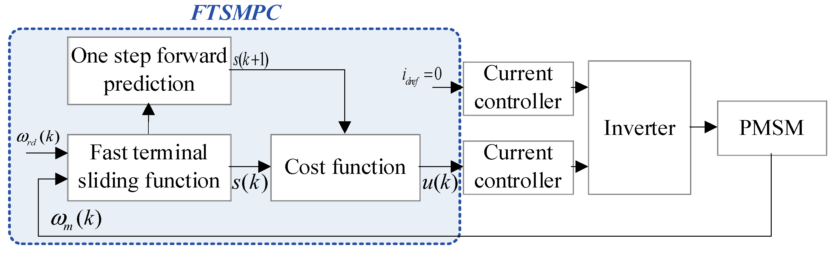
First, to enhance the convergence performance of the system states, a fast terminal sliding function is established. Then, one-step forward prediction is made for the sliding function. The error between the expected and the real sliding function is defined by a cost function. Based on one-step optimization, the control of the sliding function to a predetermined trajectory is obtained. The scheme of the proposed FTSMPC is shown in Figure 1.
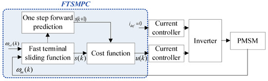
Figure 1.
The general control structure of the proposed FTSMPC for PMSM systems.
The discrete-time fast terminal sliding function at the moment k is expressed as
where , , .
The next step of the sliding function can be derived as
Then, the cost function is defined based on tracking the trajectory for , which can be expressed as (9). In addition, to have a fast convergence, a fast terminal reaching law is also employed.
where , .
The minimum value of the cost function can be obtained by taking the derivative of (9) and setting it to zero.
The output of the speed loop under the predetermined system state tracking is
The reference of the q-axis current control reference can be expressed as
3.2. Stability and Convergence Analysis
In order to illustrate the convergence of the system, the following assumption and lemma are introduced:
Assumption 1.
The derivative of disturbance is assumed to be bounded, i.e., , with a constant .
Lemma 1
([18]). For discrete systems:
where , and . If , then the state is always bounded.
Proof.
Submitting (11) into the sliding function predictive model (8) yields
It can be obtained by Assumption 3.1 that . According to Lemma 1, the sliding function defined by (7) is bounded by
When , the bound of the sliding function is majorly determined by the factor . Large will enhance the control accuracy but results in slow convergence [18]. To balance the control accuracy and the convergence rate, is selected as , which leads to (18) under no load. □
When , the bound of the sliding function is majorly determined by the factor and , which can be expressed as (19). is still selected as 2/3 and the bound of will increase as the increases, which will change the control volume to allow it to resist external disturbances. When the disturbances disappear, the bound of the sliding function can still change to (18).
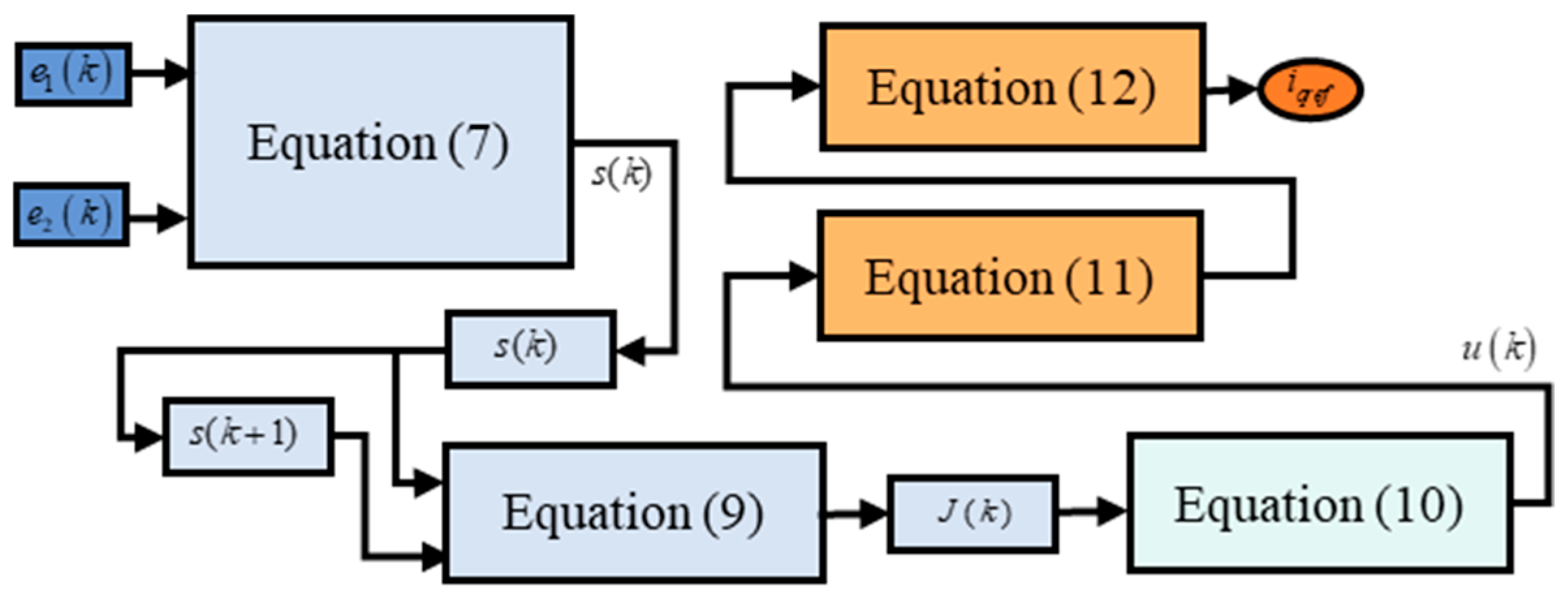
The structure of the proposed FTSMPC is shown in Figure 2.
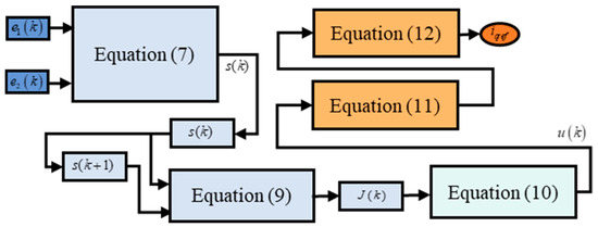
Figure 2.
The specific structure of FTSMPC for PMSM speed control.
The system state’s sliding function of the proposed FTSMPC can be expressed in continuous time.
The time for the system state to converge to zero can be obtained by solving the equation .
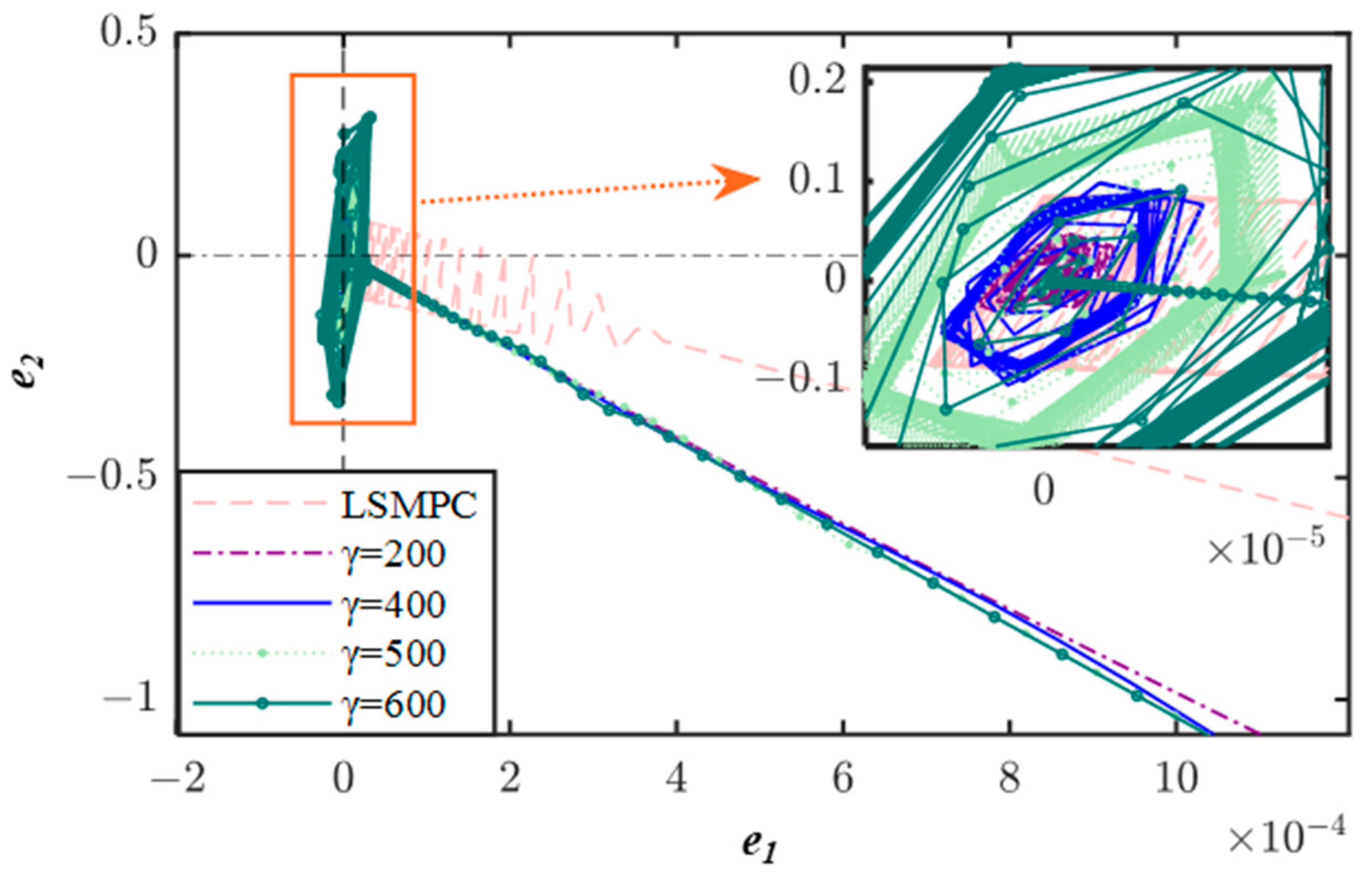
The convergence time is majorly affected by the initial value of the system state and the parameters of the sliding function. Large c1 and γ will enhance the convergence rate but will also lead to a jitter. The comparison of the system state’s convergence performance for LSMPC and FTSMPC under different γ and the same c1 is shown in Figure 3. A large γ will speed up the process.
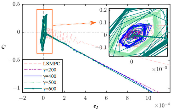
Figure 3.
The convergence performance of FTSMPC with different γ.
4. Simulation and Experimental Analysis
In this section, numerical simulations and experiments are employed to verify the effectiveness of the proposed speed control method. The design of the comparison speed controller is introduced. The speed control performance of the PI, LSMPC and FTSMPC will be compared. The system parameters of the PMSM considered in simulations are given in Table 1.

Table 1.
Parameters of the PMSM.
4.1. Design of PI and LSMPC Speed Controller
4.1.1. Design of PI Speed Controller
According to [21], the PI speed controller can be designed as
where and represent the proportional and integral factors, respectively; expresses the bandwidth of the speed control; B is the active damping.
4.1.2. Design of LSMPC Speed Controller
Based on a second-order discrete system, a linear sliding function can be selected as
The next moment sliding function can be obtained by one-step forward prediction.
To make the predictive sliding function approximate the target trajectory, the cost function is designed based on linear reaching law.
The optimal current control command can be derived by solving .
Under the traditional LSMPC, the reference of the q-axis current control reference can be expressed as
4.2. Simulations and Experiments
4.2.1. Parameter Tuning
The parameter tunning process of the proposed FTSMPC, the traditional PI, and the conventional LSMPC is introduced in this section.
FTSMPC Speed Controller: Large c1 and γ can speed up the convergence rate of the system state. The system will chatter and the control accuracy will be lower along with the larger c1 and γ. c1 can be chosen as 100 initially and gradually increase by 50 until system jittering occurs, where the optimal c1 is the value that makes the system jitter-free. The c1 is selected as 500 and 200 in during simulations and experiments when tuned by the above method. The value of γ has been discussed in Section 3. and affect the anti-disturbance capability of the system and can be selected from 0 to 1. Larger and will enhance the system robustness but cause jitter and low accuracy. To balance the accuracy and the robustness, and are chosen as 0.8 and 0.8, respectively.
LSMPC Speed Controller: Like FTSMPC, the convergence rate of the system states will enhance with the increase in c1. If c1 is too large, the system will chatter and the control accuracy will be lower. c1 is chosen as 200 and 500 in simulations and experiments, respectively. Larger and increase the anti-disturbance capability but result in jitters in the system states. and are selected as 0.5 and 0.4 in simulations and 0.7 and 0.6 in experiments.
PI Speed Controller: The bandwidth of the PI speed controller is selected as 400. To make a fair comparison, is set in the simulation, which makes the overshoot approach zero. is adjusted to during the experiments to account for sharp jitter from excessive .
PI Current Controller: The factors of the PI current controllers on the d-q coordinate system are the same. According to [22], . To avoid the effect of the response on the speed control, is set as 4106.5 in simulations, and the factors are adjusted to the same for the experiments. To make the comparison fair, the current controllers of the PI, LSMPC and FTSMPC speed controllers are designed to be the same.
The specific parameters of the speed controllers for simulations and experiments are shown in Table 2. The proportional and integral parameters of the speed controller are the same for the PI, LSMPC and FTSMPC. Control parameters are adjusted during the experiment for the mechanical connection. The mechanical connection results in differences in inertia and static friction from the theory, which makes the control parameters different between experiments and simulations.
Table 2.
Parameters of the controllers.
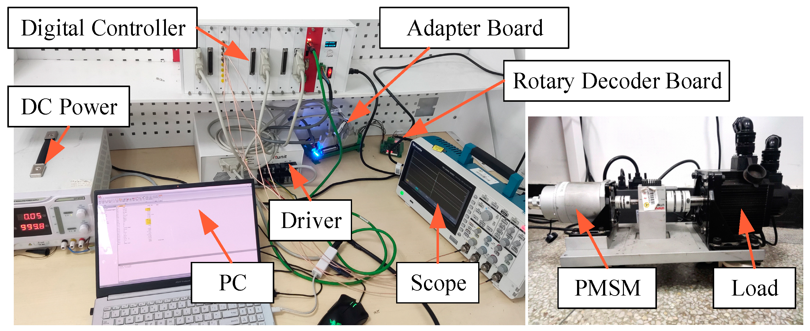
The setup configuration of the experiment is displayed in Figure 4, which is mainly composed of a PMSM, a real-time digital controller based on a digital signal processor (DSP, TMS320F28335), an RTU control platform, a computer with MATLAB R2022b/Simulink, a rotary encoder, a driver and DC power supplies. The final control program is directly generated from the MATLAB/Simulink program and burned in TMS320F28335 by the RTU control platform. The sample period Ts is chosen as 0.0001 s. The PWM frequency is set as 10 kHz. The PMSM parameters for the experiments are same as those for the simulations.
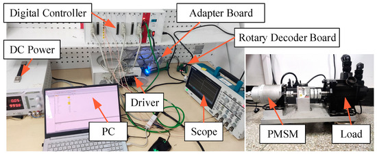
Figure 4.
Experimental setup.
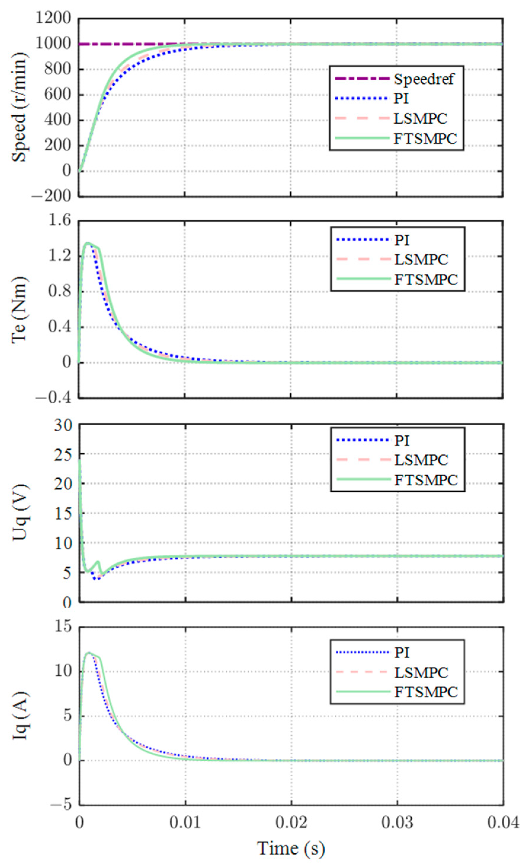
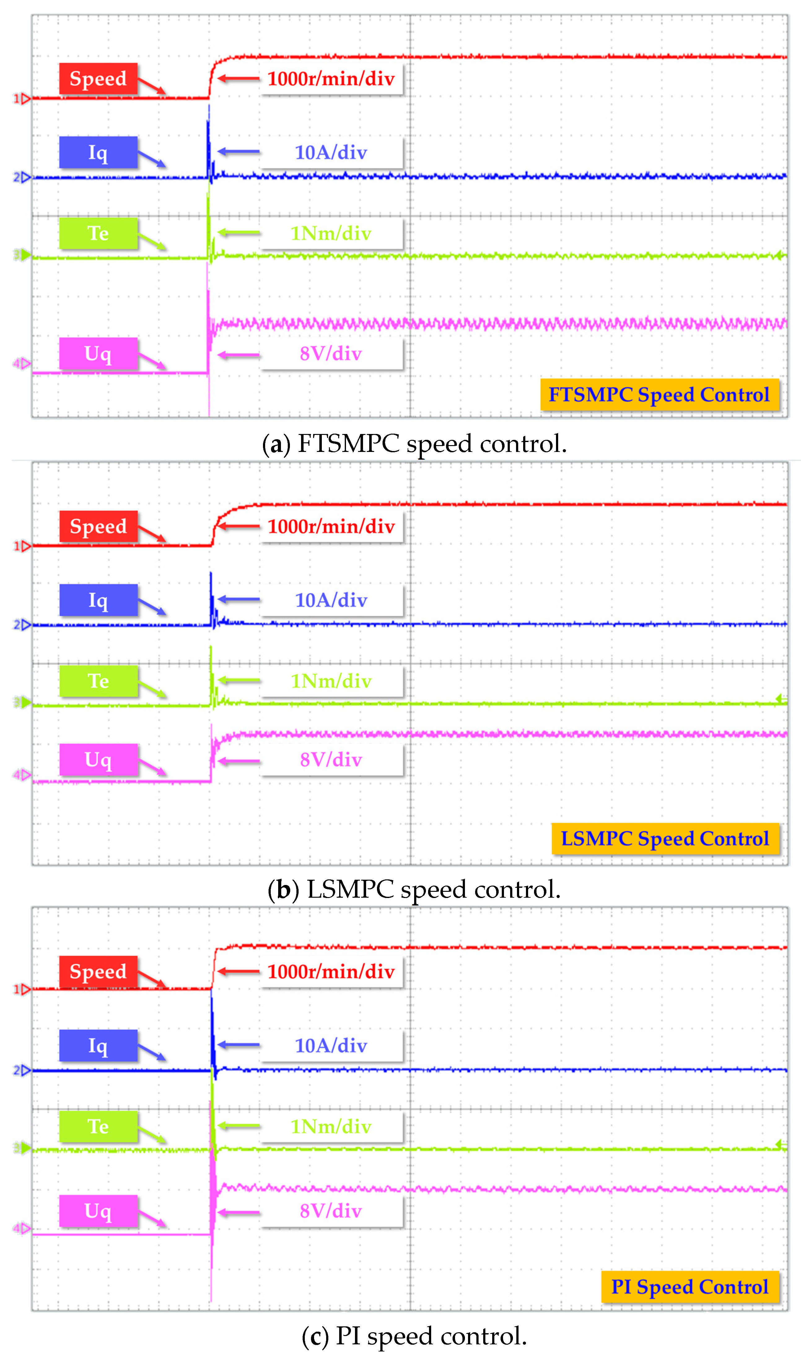
4.2.2. Step Response Performance
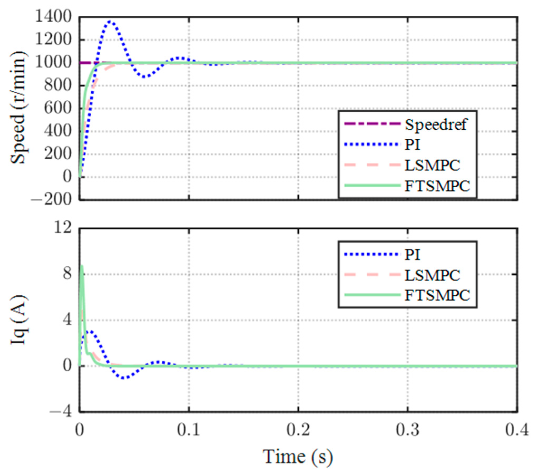
Figure 5 and Figure 6 and Table 3 are the results of the step response test under the simulation and experiment for the PI, LSMPC and FTSMPC speed controllers. No load is added in this test. As shown in Table 3, the proposed FTSMPC has a close rise time to the PI control and a shorter settling time than both the LSMPC and PI control. The overshoot of the FTSMPC and LSMPC controllers is zero in the simulation and experiment. It is not easy for the PI to avoid overshooting under the experiment, which is 5.51% the speed reference. It can be concluded that the proposed FTSMPC has a faster convergence rate than the LSMPC and PI control. The dynamic convergence performance of FTSMPC is better than the other two methods.
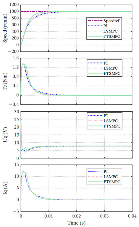
Figure 5.
Simulation results of the step response performance comparisons.

Figure 6.
Experimental results of the step response performance comparisons.
Table 3.
Step response performance comparison.
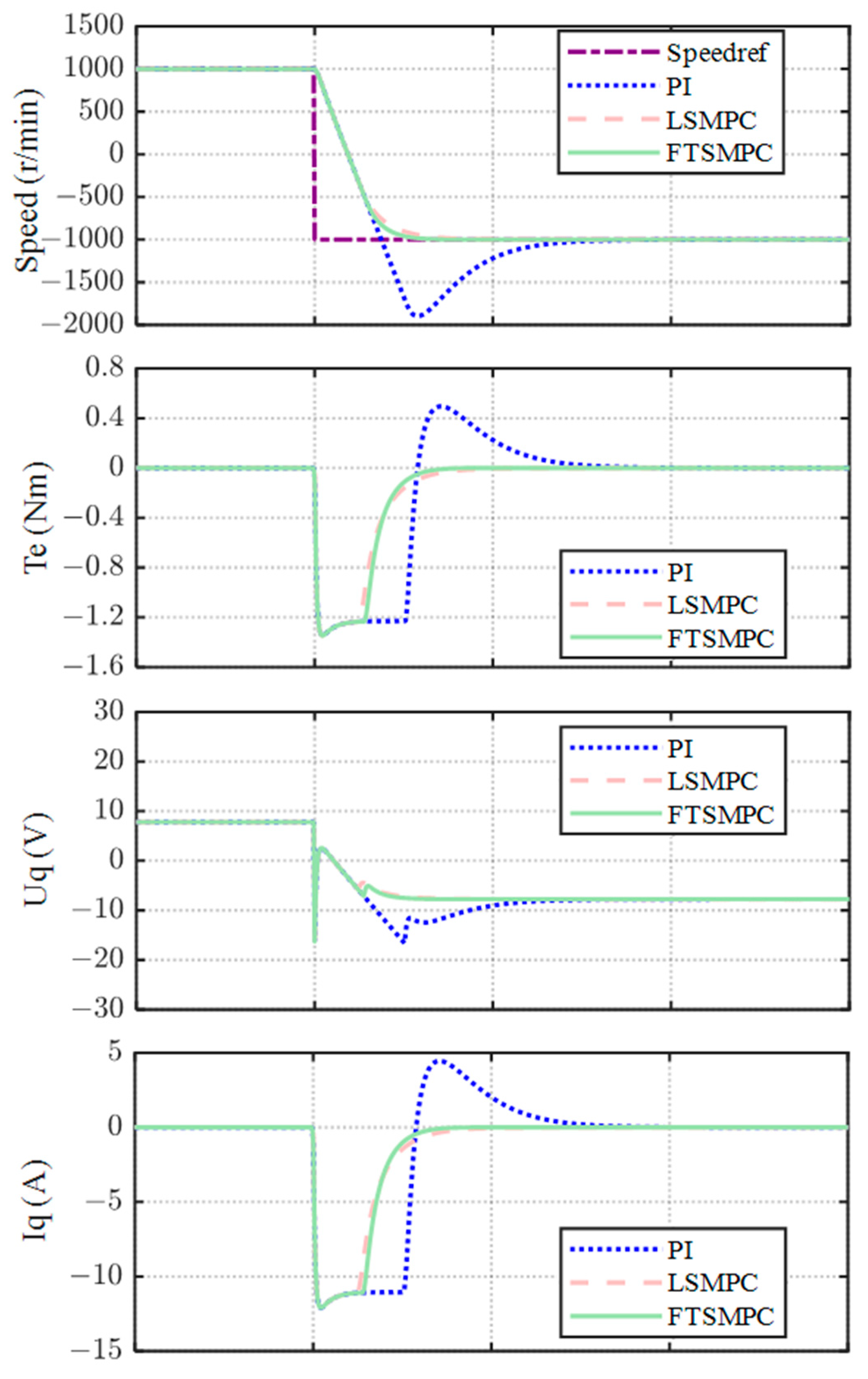
4.2.3. Speed Revisal Performance
The performance comparisons of the PI, LSMPC and FTSMPC under the speed revisal test in the simulation and experiment are shown in Figure 7 and Figure 8 and Table 4. The reference speed is initialized to 1000 r/min and then is suddenly set to −1000 r/min. Obviously, the rise time of the PI is shorter than that of LSMPC and FTSMPC. However, the excessive response of the PI leads to a large overshoot, which causes a long settling time. It can be concluded from Table 4 that the settling time of FTSMPC is shorter than that of the other two controllers in the simulation and experiment. During the stage of nonlinear convergence, the system states converge faster under FTSMPC than under the PI and LSMPC. Overall, FTSMPC displays better dynamic performance, especially in terms of settling time.
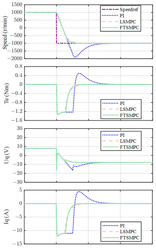
Figure 7.
Simulation results of the speed revisal performance comparisons.
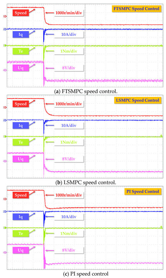
Figure 8.
Experimental results of the speed revisal performance comparisons.
Table 4.
Speed revisal performance comparison.
4.2.4. Load Disturbance Performance
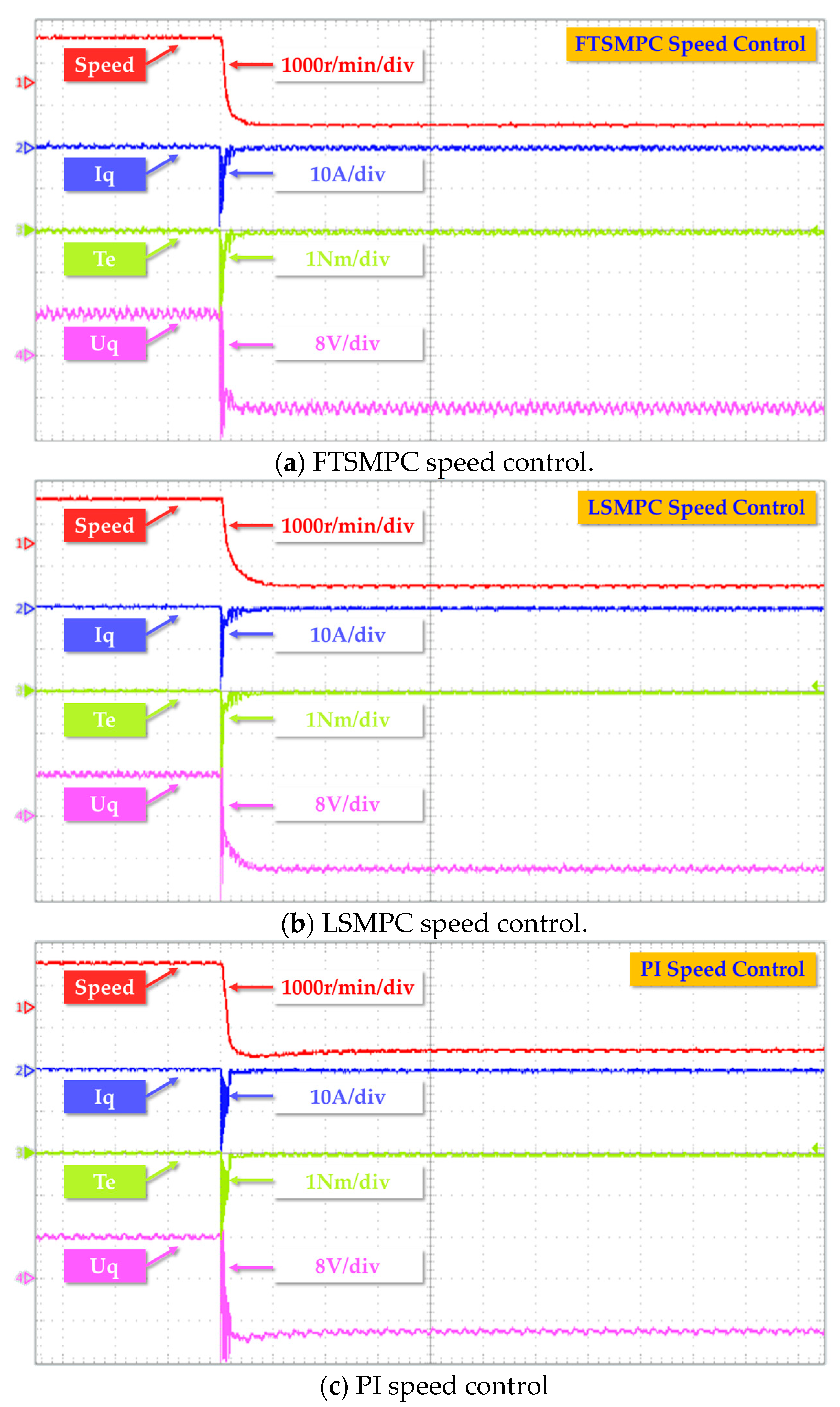
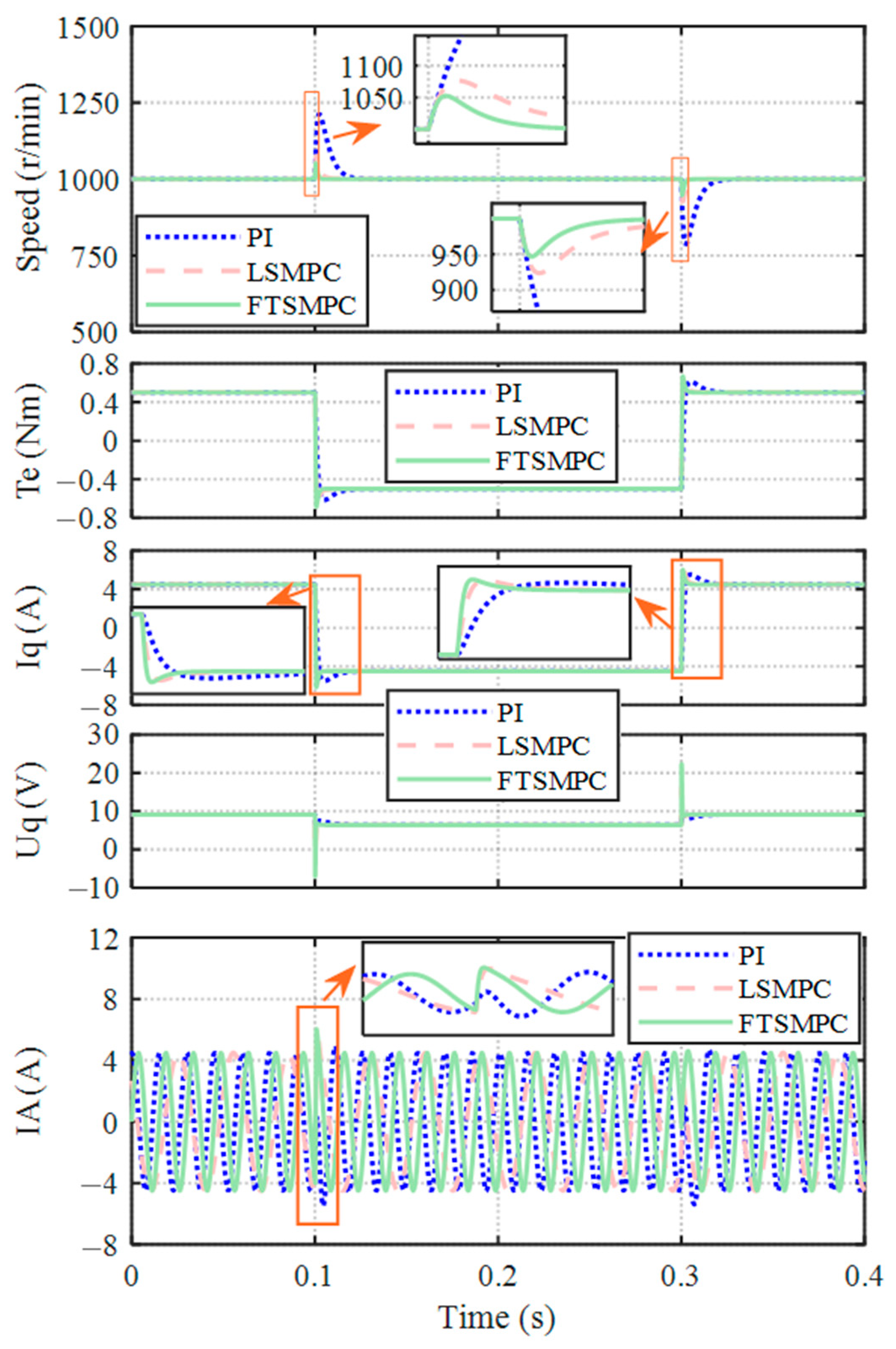
As shown in Figure 9, the rotor speed reference is fixed at 1000 r/min during this test. The PMSM runs with 0.5 Nm load at the initial time, and then, the load is abruptly revised to −0.5 Nm and 0.5 Nm at 0.1 s and 0.3 s, respectively. From Table 5, it can be found that FTSMPC has the shortest recovery time and the lowest overshoot and undershoot. The overshoot of FTSMPC is almost 24.7% that of the PI and 68.9% that of LSMPC. Hence, compared to the PI and LSMPC, FTSMPC has stronger robustness.
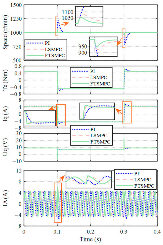
Figure 9.
Simulation results of the load disturbance performance comparisons.
Table 5.
Load disturbance performance comparison.
4.2.5. Parameter Variation Performance
The comparison results of the robustness against rotational inertia are shown in Figure 10 and Table 6. The control parameter J is ten times the PMSM parameter, and the step response test is adopted to investigate the control performance under the mismatched control parameter. The rise time and settling time of FTSMPC is still shorter than that of the PI and LSMPC. In addition, the overshoot of the PI is 359.68 r/min, while that of LSMPC and FTSMPC is zero. So, FTSMPC has stronger robustness against the control parameter J than the PI and LSMPC.
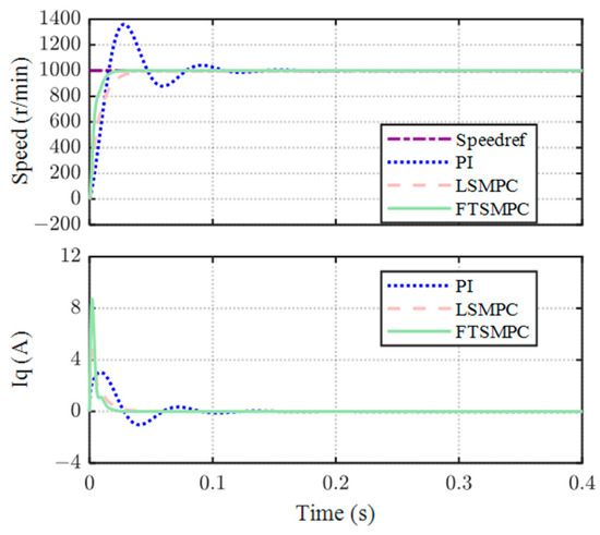
Figure 10.
Simulation results of the parameter variation performance comparisons.
Table 6.
Parameter variation performance comparison.
Through simulations and experiments, it can be demonstrated that FTSMPC has better convergence performance compared to the traditional LSMPC and PI control, especially in the nonlinear convergence stage of the system states.
5. Conclusions
This paper has proposed a FTSMPC algorithm to increase the convergence rate of PMSM systems. Compared to the traditional LSMPC and PI control, the convergence rate of the nonlinear stage is increased under FTSMPC, resulting in a better convergence performance. The validity of the proposed method is verified by convergence analysis, simulations and experiments. The simulation and experimental results show that FTSMPC is superior to the PI and LSMPC in convergence performance and robustness against external disturbances.
Author Contributions
Conceptualization, D.K. and H.C.; methodology, D.K.; software, D.K.; validation, D.K., H.C. and W.Z.; formal analysis, D.K.; investigation, D.K.; resources, H.C.; data curation, W.Z.; writing—original draft preparation, D.K.; writing—review and editing, D.K. and H.C; visualization, W.Z.; supervision, H.C.; project administration, H.C.; funding acquisition, H.C. All authors have read and agreed to the published version of the manuscript.
Funding
This research was funded by the National Natural Science Foundation of China (NO. 51991383, 52107038).
Data Availability Statement
Data are contained within the article.
Conflicts of Interest
The authors declare no conflicts of interest.
References
- Wang, H.; Jiao, T.; Xing, X.; Yang, Y. Speed Regulation of PMSM Systems Based on a New Sliding Mode Reaching Law. IEEE Access 2024, 12, 24062–24070. [Google Scholar] [CrossRef]
- Rovere, L.; Formentini, A.; Zanchetta, P. FPGA Implementation of a Novel Oversampling Deadbeat Controller for PMSM Drives. IEEE Trans. Ind. Electron. 2019, 66, 3731–3741. [Google Scholar] [CrossRef]
- Zuo, Y.; Lai, C.; Iyer, K.L.V. A Review of Sliding Mode Observer Based Sensorless Control Methods for PMSM Drive. IEEE Trans. Power Electron. 2023, 38, 11352–11367. [Google Scholar] [CrossRef]
- Lara, J.; Xu, J.; Chandra, A. Effects of Rotor Position Error in the Performance of Field Oriented Controlled PMSM Drives for Electric Vehicle Traction Applications. IEEE Trans. Ind. Electron. 2016, 63, 4738–4751. [Google Scholar] [CrossRef]
- Seok, J.K.; Lee, J.K.; Lee, D.C. Sensorless speed control of nonsalient permanent-magnet synchronous motor using rotor-position-tracking PI controller. IEEE Trans. Ind. Electron. 2006, 53, 399–405. [Google Scholar] [CrossRef]
- Li, X.; Tian, W.; Gao, X.; Yang, Q.; Kennel, R. A Generalized Observer-Based Robust Predictive Current Control Strategy for PMSM Drive System. IEEE Trans. Ind. Electron. 2022, 69, 1322–1332. [Google Scholar] [CrossRef]
- Yim, J.; You, S.; Lee, Y.; Kim, W. Chattering Attenuation Disturbance Observer for Sliding Mode Control: Application to Permanent Magnet Synchronous Motors. IEEE Trans. Ind. Electron. 2023, 70, 5161–5170. [Google Scholar] [CrossRef]
- Garduno, D.; Rivas, J.J.; Castillo, O.; Ortega Gonzalez, R.; Gutierrez, F.E. Current Distortion Rejection in PMSM Drives Using an Adaptive Super-Twisting Algorithm. IEEE Trans. Energy Convers. 2022, 37, 927–934. [Google Scholar] [CrossRef]
- Nguyen, N.-D.; Nam, N.N.; Yoon, C.; Lee, Y.I. Speed Sensorless Model Predictive Torque Control of Induction Motors Using a Modified Adaptive Full-Order Observer. IEEE Trans. Ind. Electron. 2022, 69, 6162–6172. [Google Scholar] [CrossRef]
- Li, L.; Pei, G.; Liu, J.; Du, P.; Pei, L.; Zhong, C. 2-DOF Robust H∞ Control for Permanent Magnet Synchronous Motor with Disturbance Observer. IEEE Trans. Ind. Electron. 2021, 36, 3462–3472. [Google Scholar] [CrossRef]
- Shao, M.; Deng, Y.; Li, H.; Liu, J.; Fei, Q. Robust Speed Control for Permanent Magnet Synchronous Motors Using a Generalized Predictive Controller with a High-Order Terminal Sliding-Mode Observer. IEEE Access 2019, 7, 121540–121551. [Google Scholar] [CrossRef]
- Tian, M.; Wang, T.; Yu, Y.; Dong, Q.; Wang, B.; Xu, D. Integrated Observer-Based Terminal Sliding-Mode Speed Controller for PMSM Drives Considering Multisource Disturbances. IEEE Trans. Ind. Electron. 2024, 39, 7968–7979. [Google Scholar] [CrossRef]
- Wang, C.; Liu, F.; Xu, J.; Pan, J. An SMC-Based Accurate and Robust Load Speed Control Method for Elastic Servo System. IEEE Trans. Ind. Electron. 2024, 71, 2300–2308. [Google Scholar] [CrossRef]
- Zhang, L.; Chen, Z.; Yu, X.; Yang, J.; Li, S. Sliding-Mode-Based Robust Output Regulation and Its Application in PMSM Servo Systems. IEEE Trans. Ind. Electron. 2023, 70, 1852–1860. [Google Scholar] [CrossRef]
- Tian, Z.; Yuan, J.; Zhang, X.; Kong, L.; Wang, J. Modeling and sliding mode predictive control of the ultra-supercritical boiler-turbine system with uncertainties and input constraints. ISA Trans. 2018, 76, 43–56. [Google Scholar] [CrossRef] [PubMed]
- He, L.; Wang, F.; Ke, D. FPGA-Based Sliding-Mode Predictive Control for PMSM Speed Regulation System Using an Adaptive Ultralocal Model. IEEE Trans. Ind. Electron. 2021, 36, 5784–5793. [Google Scholar] [CrossRef]
- Ma, Y.; Li, D.; Li, Y.; Yang, L. A Novel Discrete Compound Integral Terminal Sliding Mode Control with Disturbance Compensation For PMSM Speed System. IEEE/ASME Trans. Mechatron. 2022, 27, 549–560. [Google Scholar] [CrossRef]
- Du, H.; Chen, X.; Wen, G.; Yu, X.; Lu, J. Discrete-Time Fast Terminal Sliding Mode Control for Permanent Magnet Linear Motor. IEEE Trans. Ind. Electron. 2018, 65, 9916–9927. [Google Scholar] [CrossRef]
- Xu, Q. Digital Integral Terminal Sliding Mode Predictive Control of Piezoelectric-Driven Motion System. IEEE Trans. Ind. Electron. 2016, 63, 3976–3984. [Google Scholar] [CrossRef]
- Kang, S.; Wu, H.; Yang, X.; Li, Y.; Yao, J.; Chen, B.; Lu, H. Discrete-Time Predictive Sliding Mode Control for a Constrained Parallel Micropositioning Piezostage. IEEE Trans. Syst. Man Cybern. Syst. 2022, 52, 3025–3036. [Google Scholar] [CrossRef]
- Zhang, X.; Wang, Z.; Bai, H. Sliding-Mode-Based Deadbeat Predictive Current Control for PMSM Drives. IEEE J. Emerg. Sel. Top. Power Electron. 2023, 11, 962–969. [Google Scholar] [CrossRef]
- Yang, S.-M.; Lin, K.-W. Automatic Control Loop Tuning for Permanent-Magnet AC Servo Motor Drives. IEEE Trans. Ind. Electron. 2016, 63, 1499–1506. [Google Scholar] [CrossRef]
Disclaimer/Publisher’s Note: The statements, opinions and data contained in all publications are solely those of the individual author(s) and contributor(s) and not of MDPI and/or the editor(s). MDPI and/or the editor(s) disclaim responsibility for any injury to people or property resulting from any ideas, methods, instructions or products referred to in the content. |
© 2024 by the authors. Licensee MDPI, Basel, Switzerland. This article is an open access article distributed under the terms and conditions of the Creative Commons Attribution (CC BY) license (https://creativecommons.org/licenses/by/4.0/).