Numerical Investigation of Hydraulic Fractures Vertical Propagation Mechanism for Enhanced Tight Gas Recovery

Abstract

Hydraulic fracturing stands as a pivotal technological approach for enhanced tight gas recovery. This paper investigates the influences of geological and engineering parameters on the vertical extension mechanism of hydraulic fractures. In addition, the feasibility and effectiveness of fracture height prediction method and various fracture height control techniques have been examined. The results indicate that the height of hydraulic fractures decreases with an increase in the thickness of the barrier layers, the stress difference between the barrier and reservoir layers, the difference in tensile strength, and the difference in fracture toughness, whereas it increases with the increasing of difference in elastic modulus between the barrier and reservoir layers. Compred with the difference in Poisson’s ratio, the volume of fracturing fluid, discharge rate, and fluid viscosity have little impactd. The influence of these factors on fracture height, in descending order, is stress difference between barrier and reservoir layers, fracturing fluid viscosity, fracturing discharge, fracturing fluid volume, barrier layer thickness, tensile strength difference between barrier and reservoir layers, elastic modulus difference between barrier and reservoir layers, Poisson’s ratio difference between barrier and reservoir layers. Furthermore, based on typical geomechanic and reservoir parameters of the target area, a fracture height prediction workflow has been developed. Engineering practice has proven the reliability of fracture height prediction method. The results of this study provide theoretical support and guidance for predicting fracture morphology, controlling fracture height in the hydraulic fracturing development of the tight gas reservoir, and optimizing fracturing process design.

1. Introduction

With the continuous development and exploration of China’s oil industry, unconventional oil and gas resources are gradually becoming the mainstay for the succession of oil and gas resources. The Linxing–Shenfu tight gas block, as a key area for unconventional oil and gas resources onshore for CNOOC (China National Offshore Oil Corporation), has significant implications for enhancing reserves and boosting production. Currently, hydraulic fracturing has become a key technical approach for increasing production in that block.

The hydraulic fracturing process becomes gaining more popularity to increase production in tight sandstone gas reservoirs. When there are no barriers above or below the target layer, or if existing barriers do not have sufficient stress differences and thickness, hydraulic fractures can easily extend vertically into non-target layers, leading to increased fracture heights. This not only fails to achieve the goal of deep penetration and long fracture creation but also wastes proppants and fracturing fluid, increasing the cost of fracturing. Additionally, if fractures vertically connect with aquifers or coal seams and other risk layers, it may lead to serious water-invasion phenomenon in gas wells, inducing “water block” or pressure propagation into other layers, which severely impacts the effectiveness of fracturing. Therefore, during fracturing design, it is necessary to predict the vertical expansion and the morphology of hydraulic fractures and reasonably control the fracture height through technical means to avoid uncontrolled fracture heights.

Naceur et al. [1] believe that the factors affecting the vertical extension of hydraulic fractures can be divided into two major categories: uncontrollable geological factors and controllable engineering operational factors. The reservoir geomechanics and rock physical properties will inevitably affect the behavior of the vertical extension of hydraulic fractures. Simonson et al. [2] claim that the vertical extension behavior of hydraulic fractures is mainly influenced by the stress difference between layers; Through the establishment of a three-dimensional fracture extension mathematical model, Huang et al. [3] found that the fracture height decreases significantly as the stress difference between layers increases; Through laboratory experiments, Warpinski et al. [4] summarized that when the stress difference between layers reaches 4 to 6 MPa, it can restrict the cross-layer propagation of fractures. Gu et al. [5,6] found that the difference in the elastic modulus between the barrier and reservoir layers is another main factor affecting fracture height, in addition to the stress difference between layers. It is believed that a high elastic modulus barrier layer will promote the vertical expansion of the fracture. Van Eekelen [7] clarifies that if the elastic modulus of the interlayer is high, the vertical expansion of fractures will be inhibited; Smith et al. [8] believe that the difference in elastic modulus between barrier and reservoir layers alone is insufficient to affect vertical fracture propagation. Huang et al. [9] and Salah et al. [10] believed that the plastic behavior of the interlayer is manifested as the Poisson’s ratio, with a larger Poisson’s ratio having a greater impact on the fracture height; Li et al. [11] believes that compared to the stress difference between layers, the difference in the Poisson’s ratio of the barrier/capacity layer on the vertical expansion of fractures can be negligible. Gao et al. [12] and Detounay [13] believe that the toughness of rock fractures also has little influence on fracture height, while Chen et al. [14], based on the theoretical methods of rock mechanics, have deduced that fracture toughness plays a significant role in arresting the vertical expansion of fractures. Qin et al. [15] and Cong et al. [16] found through numerical simulation studies that the greater the tensile strength of the barrier layer, the smaller the fracture height.

In addition to the geological rock properties, the height of hydraulic fractures is also influenced by engineering parameters such as fracturing displacement, fluid volume, and viscosity. Through comparing well temperature data before and after fracturing operations across multiple blocks, Tang et al. [17] have summarized an empirical formula that fracture height increases as the fracturing displacement; Kresse et al. [18] conducted numerical simulation to study that the larger the displacement, the easier to achieve vertical cross-layer expansion. Based on the mechanism of horizontal fracture expansion and fluid flow equations, Mehrabi et al. [19] have found that there is a positive correlation between the amount of fracturing fluid and the discharge rate and fracture height, with a significant impact; Rho et al. [20] believe that the influence of construction scale on fracture height is second only to the interlayer stress difference. Yang et al. [21] used the finite element numerical discretization method to study the relationship between fracturing fluid viscosity and fracture height. The results showed that the higher the viscosity, the easier it is for the fracture to penetrate the layers and enter the interspace, and the higher the viscosity, the greater the fracture height after layer penetration; Du et al. [22] found that as viscosity increases, fracture height gradually increases, while fracture length and fracture width gradually decrease; however, Li et al. [23] prove that as viscosity increases, fracture length decreases, while fracture width and fracture height gradually increase.

In summary, the geology and engineering parameters have a significant impact on the vertical expansion of hydraulic fractures, but there is still some controversy over the understanding of the impact of each factor on the vertical expansion of fractures, and the degree of impact of each factor on fracture height is not yet clear. Hence, this paper will further study the impact rules of different geological and engineering factors on the vertical expansion of hydraulic fractures in practice of Linxing–Shenfu tight gas reservoir and further clarify the main controlling factors of fracture height. In addition, we also establish a method for predicting fracture height and propose technical measures to control the excessive extension of fracture height. Thus, two aspects related to the vertical expansion of hydraulic fractures are as follows:

• Numerical simulation methods are used to explore the vertical expansion law of hydraulic fractures from two aspects: geological lithology and engineering operation. The consodered geological factors mainly consist of barrier/reservoir stress, thickness, elastic modulus, Poisson’s ratio, tensile strength, and the difference in fracture toughness; The engineering factors mainly include fracturing fluid volume, discharge, and viscosity which are verified through laboratory experiments as well;
• Based on the influence pattern and extent of various factors on the vertical extension of hydraulic fractures, we clarify the main controlling factors of fracture height and establish the fracture height prediction map. Finally, the feasibility and effect of three fracture height control technologies, e.g., multi-stage intermittent sand addition, low-viscosity pre-fluid, and multi-stage variable-displacement, are verified through field application.

In summary, based on the hydraulic fracturing practices in the tight gas block, this paper explores the influences of geological and engineering factors on the vertical extension behavior of hydraulic fractures. The key factors controlling the height of the fracture are clarified and a fracture height prediction method is established. Targeted fracture height control techniques are proposed, providing guidance for the optimization of fracturing design and the improvement of fracturing processes in the area. This contributes to efficient fracturing development in the tight gas reservoirs.

2. Research on the Vertical Expansion Law of Hydraulic Fractures

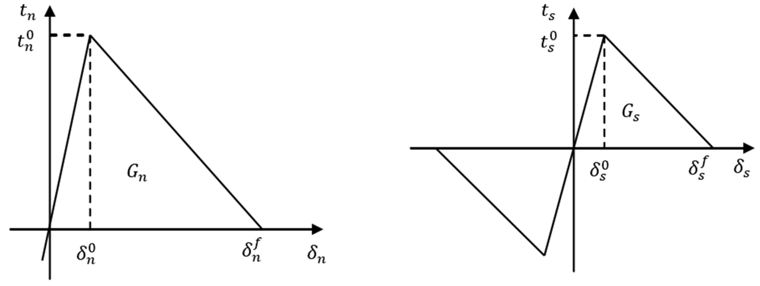
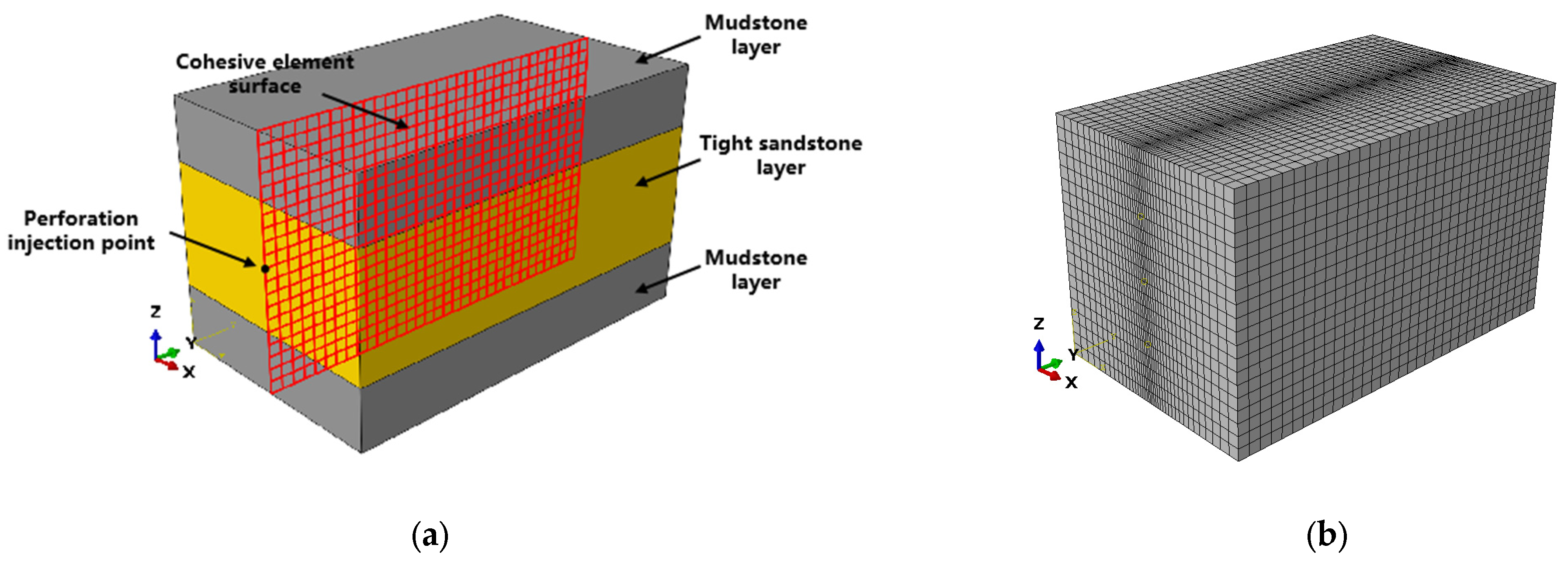
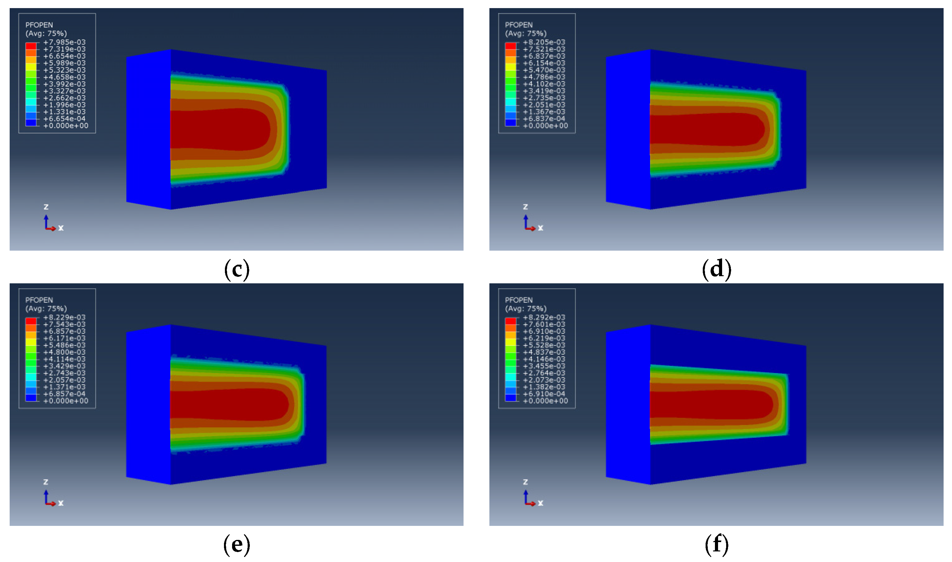
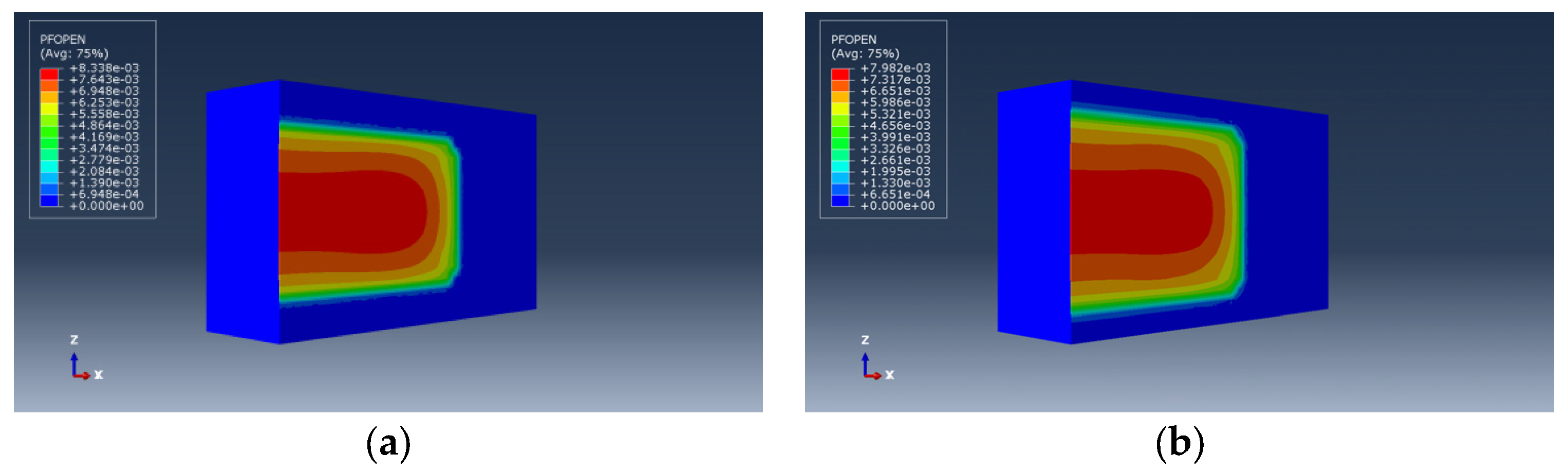
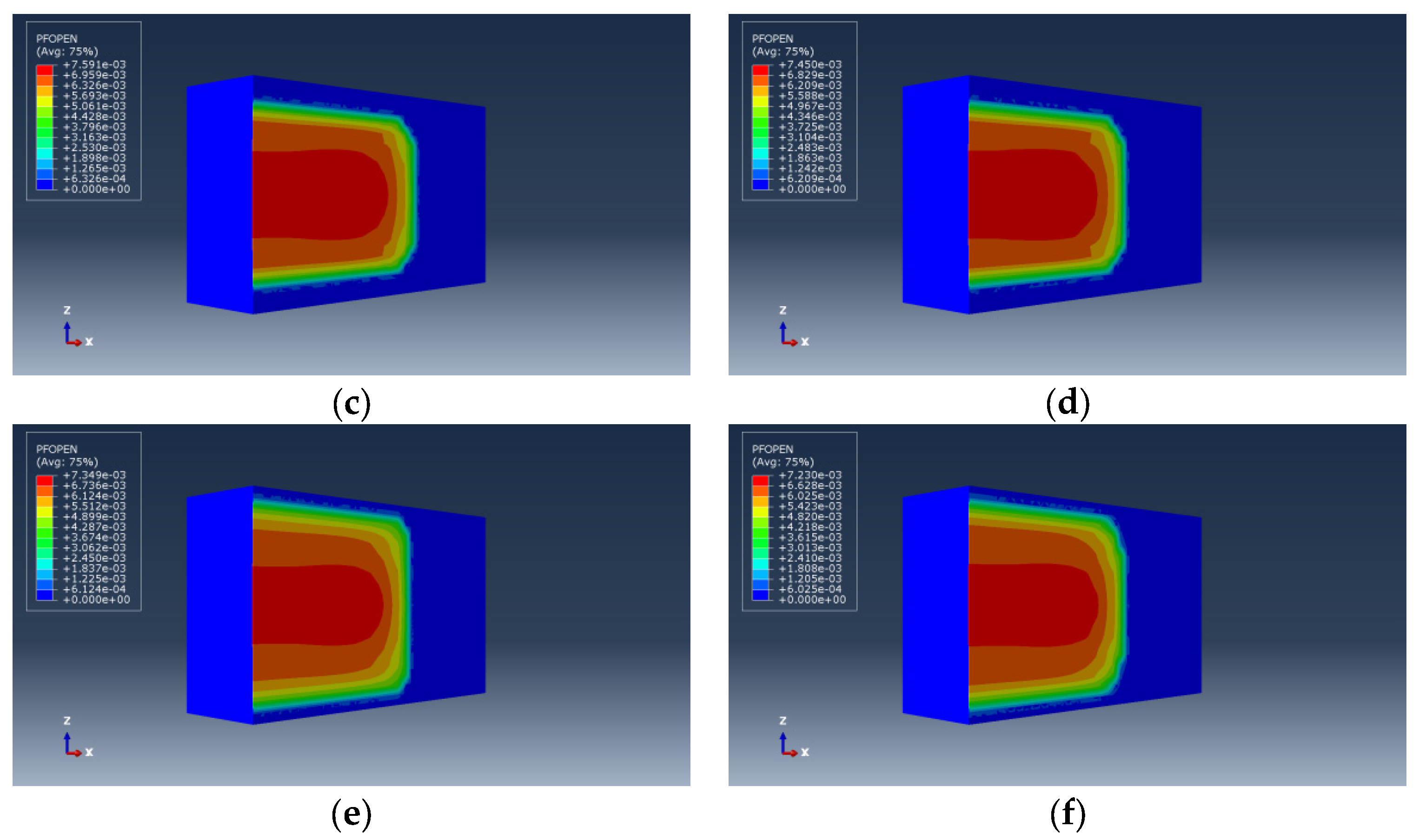
2.1. Establishment of Numerical Models

(1) Model settings

The numerical model for vertical expansion of hydraulic fractures in this paper is based on damage mechanics and the finite element framework. It uses stiffness degradation of the cohesive element to simulate the initiation and expansion of hydraulic fractures. However, considering the complexity and variability of the actual hydraulic fracturing process and the mechanical state of the formation rocks, the following assumptions are made in the model for the convenience of simulation and calculation:

① A damage factor is used to simulate the damage evolution at the fracture front, and the quadratic nominal stress criterion is used to simulate fracture propagation and extension;

② The formation rock is considered a homogeneous, isotropic, linear elastic porous medium;

③ Ignore the effect of the temperature field on fracture propagation;

④ The fracturing fluid is incompressible and fully saturated; during the fracturing process, neither the physicochemical interactions between the fracturing fluid and the surrounding rocks nor the inertial effects of the fluid itself are considered. Moreover, the tangential flow of the fracturing fluid during the fracture propagation process is simulated based on the cubic law. Additionally, a fracturing fluid leak-off coefficient on the fracture surface is introduced to simulate the normal leak-off of the fluid from the fracture into the surrounding rock matrix on both sides.

(2) Model governing equation

① Fracture initiation criterion

Damage modeling can be used to simulate the degradation and ultimate failure of the strengthening elements. The failure mechanism consists of two components: the damage initiation criterion and the damage evolution law. As shown in Figure 1, the bilinear traction–separation constitutive model of element stiffness degradation realizes the damage evolution of the cohesive element and then simulates the fracture initiation and propagation. Before the onset of damage, the element’s constitutive relationship is linear elastic. Once the damage criterion is met, the element’s stiffness gradually degrades until it loses its load-bearing capacity.

The initiation criterion of the cohesive element adopts the quadratic nominal stress criterion; it is defined as follows:

$${\left({\displaystyle \frac{〈t_n〉}{t_n^0}}\right)}^2+{\left({\displaystyle \frac{〈t_{s1}〉}{t_{s1}^0}}\right)}^2+{\left({\displaystyle \frac{〈t_{s2}〉}{t_{s2}^0}}\right)}^2=1$$

(1)

where $t_n$ is the normal nominal stress of the cohesive element, $t_{s1}$ is the first tangential nominal stress of the cohesive element, and $t_{s2}$ is the second tangential nominal stress of the cohesive element. $t_n^0$, $t_{s1}^0, t_{s2}^0$ are the corresponding critical normal nominal stress, critical first tangential nominal stress, and critical second tangential nominal stress, respectively. The symbol “< >” means that the cohesive element does not undergo damage under compressive stress or strain; it is defined as follows:

$$〈t_n〉=\left\{\begin{array}{c}{t}_n,t_n\ge 0\\ 0,t_n<0\end{array}\right.$$

(2)

② Fracture propagation criterion

The damage evolution law describes the rate at which the material stiffness is degraded once the corresponding damage initiation criterion is reached. In this model, the damage evolution of the cohesive element law is described as follows:

$$t_n=\left\{\begin{array}{c}(1-D){\overline{t}}_n,t_n\ge 0\\ {\overline{t}}_n,t_n<0\end{array}\right.$$

$$t_{s1}=(1-D){\overline{t}}_{s1}$$

$$t_{s2}=(1-D){\overline{t}}_{s2}$$

(3)

where $t_n$, $t_{s1}$, $t_{s1}$ are the actual stress acting on the cohesive element, ${\overline{t}}_n$, ${\overline{t}}_{s1}$, ${\overline{t}}_{s2}$ are the stress acting on the cohesive element under undamaged stiffness conditions, and $D$ is a dimensionless damage factor with a value between 0 and 1. When $D=0$, the material is not damaged, and when $D$ = 1, the material is completely damaged. It is defined as follows:

$$D={\displaystyle \frac{{\delta }_f\left({\delta }_m-{\delta }_0\right)}{{\delta }_m\left({\delta }_f-{\delta }_0\right)}}$$

(4)

where ${\delta }_f$ is the displacement of the cohesive element at the time of complete damage, ${\delta }_m$ is the maximum displacement reached during the loading process, and ${\delta }_0$ is the displacement at the time of initial damage.

③ Fluid flow within fractures

After the cohesive element is completely damaged, fluid enters the element, exerting pressure on the fracture walls. This process simulates the propagation behavior of hydraulic fractures. As shown in Figure 2, within the damaged cohesive element, the fluid is divided into tangential and normal flows. Tangential flow promotes fracture propagation, while normal flow shows how some of the fracturing fluid penetrates into the formation.

The fluid within the cohesive element is assumed to be an incompressible Newtonian fluid, and its tangential flow is described by the Poiseuille formula:

$$q=-{\displaystyle \frac{w^3}{12\mu }}\nabla p$$

(5)

where $q$ is the tangential flow, $\nabla p$ is the pressure gradient along the length of the cohesion element, $w$ is the fracture width, and $\mu$ is the viscosity of fracturing fluid.

The filtration loss in the normal direction of the upper and lower surfaces of the cohesion element is defined as follows:

$$\left\{\begin{array}{c}{q}_t=c_t\left(p_f-p_t\right)\\ q_b=c_b\left(p_f-p_b\right)\end{array}\right.$$

(6)

where $q_t$ and $q_b$ are the normal volume flow of the upper and lower surfaces of the fracture, respectively, $c_t$ and $c_b$ are the filtration coefficients of the upper and lower surfaces, respectively, $p_f$ is the fluid pressure in the fracture, and $p_t$ and $p_b$ are pore pressures at the upper and lower surfaces, respectively.

The fluid in the cohesion element follows the mass conservation equation:

$$q{\displaystyle \frac{\partial w}{\partial t}}+\nabla ·q+q_t+q_b=Q(t)\delta \left(x,y\right)$$

(7)

where $Q\left(t\right)$ is the fracturing fluid injection rate.

(4) Model parameter setting

Based on the geophysical logging data and completion engineering practices of the infill wells in the Linxing–Shenfu block, the Shihezi formation in this block is selected as the target research formation. The formation is located at a depth of approximately 1350–1900 m, characterized by a low and gentle structural background and widespread interbedding of sandy mudstone in vertical distribution. The changes in thickness of interlayers and reservoirs within the formation vary between 3–20 m and 5–30 m, respectively. The reservoir is dominated by tight reservoirs with a porosity of 10% and permeability of 1 mD. Natural fractures are not well developed, and the hydraulic fracturing fractures are mainly in the form of single planar fractures. Figure 3 and Figure 4 are typical physical properties and rock mechanics parameters of Shihezi formation obtained from the interpretation and calculation of logging data of fractured wells in the target block.

Table 1. Tight sandstone reservoir numerical model parameter table.

Parameter Category	Parameter Name/Units	Parameter Value
Formation parameters	Simulation depth/m	1450~1520
	Porosity/%	10
	Permeability/mD	0.5
	Elastic modulus/GPa	25
	Poisson’s ratio	0.25
	Tensile strength/MPa	4
	Shear strength/MPa	34
Pressure parameters	Pore pressure/MPa	15
	Overburden stress/MPa	40
	Maximum horizontal stress/MPa	34
	Minimum horizontal stress/MPa	26
Construction parameters	Fluid volume/m3	100
	Displacement/m3∙min−1	3
	Viscosity/mPa∙s	1
	Perforation location	Mid-reservoir

and

Table 2. Numerical model parameters of shale barrier layers.

Parameter Category	Parameter Name/Unit	Parameter Value
Subsurface parameter	Porosity/%	5
	Permeability/mD	0.05
	Elastic modulus/GPa	21
	Poisson’s ratio	0.23
	Tensile strength/MPa	5
	Shear strength/MPa	35
Pressure parameter	Pore pressure/MPa	15
	Overburden stress/MPa	40
	Maximum horizontal stress/MPa	34
	Minimum horizontal stress/MPa	28

show the specific parameter settings for this model, which mainly include formation parameters, pressure parameters, and operational parameters. For different research contents, corresponding parameters are changed to carry out numerical simulation and comparative study of the patterns.

(3) Model Geometry and Mesh Setup

As shown in Figure 5a, the model adopts a fully three-dimensional stratified model, with overall dimensions of length 100 m × width 70 m × height 70 m. The middle layer consists of a tight sandstone reservoir with a thickness of 30 m, while the upper and lower layers are shale interlayers with thicknesses of 20 m each. The wellbore direction in the model is perpendicular to the interlayers, simulating the hydraulic fracturing scenario of a vertical well, and the initiation and propagation of hydraulic fractures in the formation are simulated by inserting cohesive element faces. During the simulation of the fracturing process, the fractures will propagate along the pre-set cohesive element faces. By analyzing the failure of cohesive elements, the geometric morphology of the fractures can be obtained. The model is subjected to minimum horizontal ${\sigma }_h$, maximum horizontal ${\sigma }_H$, and vertical in situ stresses ${\sigma }_V$ in the x, y, and z directions, respectively. The outer boundary of the model is set as fixed displacement and with impermeable boundary conditions.

As shown in Figure 5b, to better study the vertical propagation behavior and geometric changes of hydraulic fractures, the model adopts a transitional mesh setup. The mesh is refined around the central fracture plane and gradually coarsened towards the outer boundaries of the model, ensuring computational accuracy while maintaining efficiency.

2.2. Analysis of Single-Factor Influence on Vertical Expansion of Hydraulic Fractures

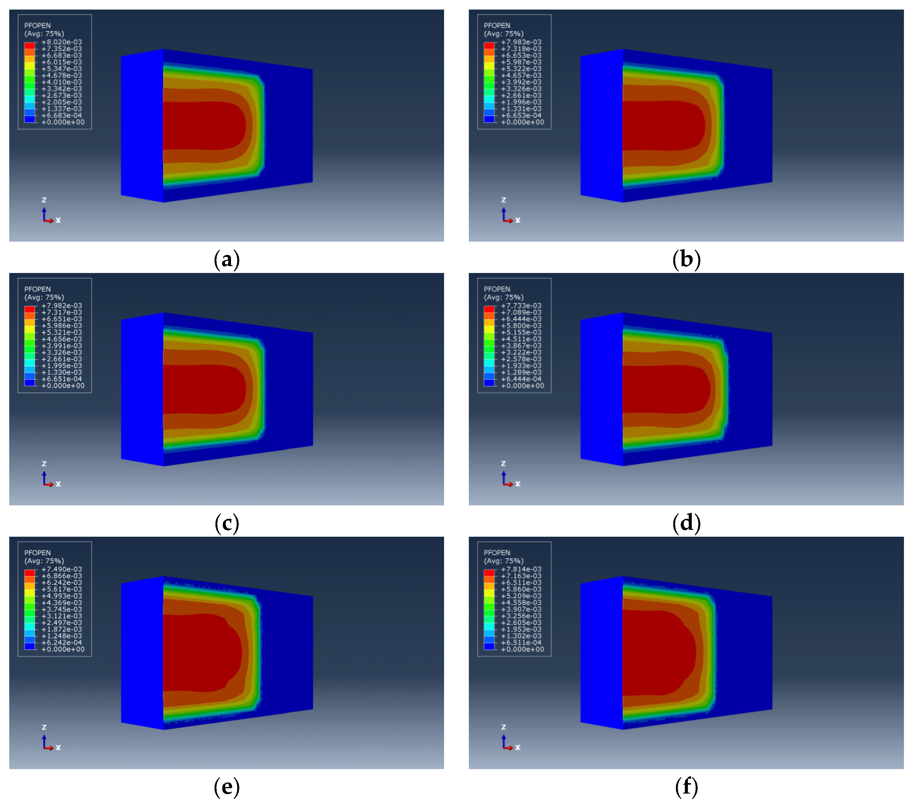
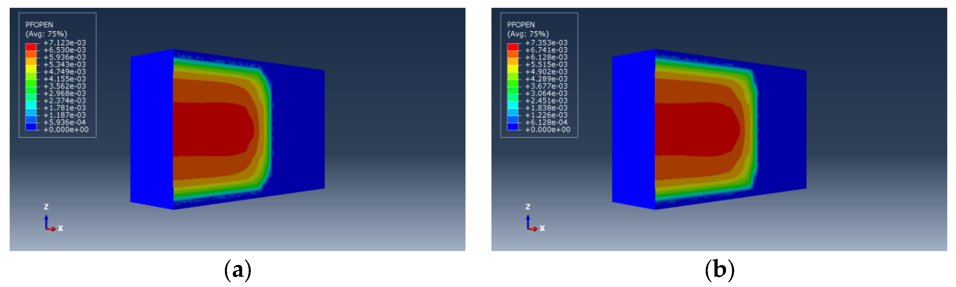
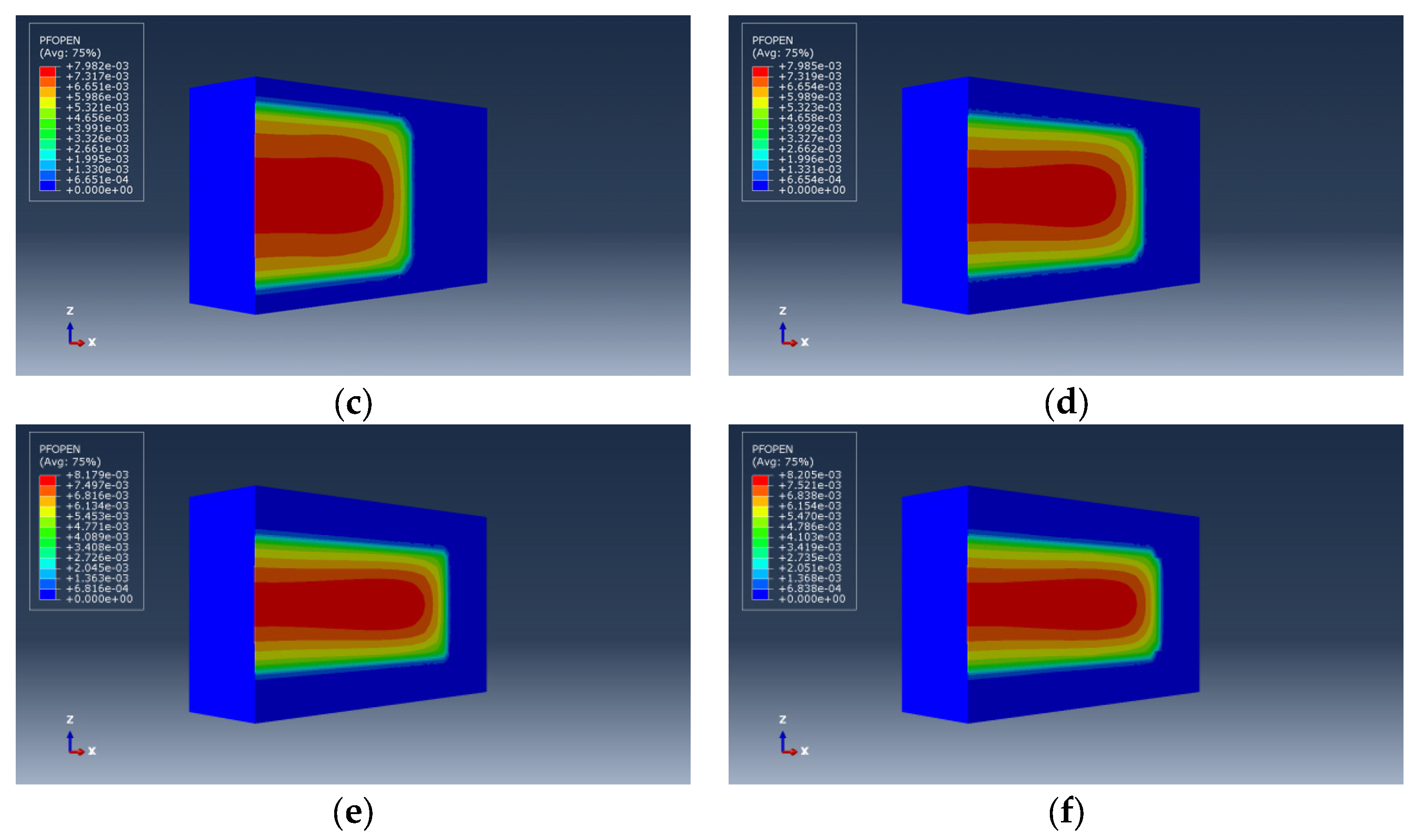
2.2.1. Influence of Geological Lithology Factors

Based on the established finite element numerical model, this section will explore the influence of differences in interlayer/strata stress, thickness, elastic modulus, Poisson’s ratio, tensile strength, and fracture toughness on the vertical expansion of hydraulic fractures.

(1) Interlayer stress difference

Change the minimum horizontal stress of the shale interlayers to 24, 26, 28, 30, 32, and 34 MPa respectively, study the influence law of the stress difference between the interlayer and reservoir layer on the vertical expansion of hydraulic fractures, and the fracture expansion morphology and calculation results are shown in Figure 6 and Figure 7, respectively.

It can be observed from Figure 3 that as the interlayer stress difference between shale interlayers and reservoir layers increases, the height of the hydraulic fractures decreases, while the length and average width of the fractures increase. This indicates that the inhibitory effect on the vertical expansion of hydraulic fractures strengthens with the increase in interlayer stress difference. When the interlayer stress difference is less than 4 MPa, a large amount of fractures penetrate into the interlayer vertically, resulting in uncontrolled fracture height. However, when the interlayer stress difference exceeds 4 MPa, the entry of fractures into the interlayer is significantly inhibited, leading to a significant reduction in fracture height. When the interlayer stress difference increases to 8 MPa, the fractures are completely confined within the reservoir, resulting in relatively larger fracture length and width. It is also observed that under constant fracturing fluid volume and formation loss, there is a trade-off relationship between fracture height, length, and width. Smaller fracture height corresponds to larger fracture length and width within the reservoir, resulting in a larger effective fracture volume. Therefore, a higher interlayer stress difference is advantageous for controlling fracture height, reducing fracturing fluid wastage, increasing the effective fracture volume within the reservoir, and improving the efficiency of reservoir stimulation.

(2) Interlayer thickness

Under the condition of an interlayer stress difference of 4 MPa, the mudstone interlayer thickness was varied to 10, 12, 14, 16, 18, and 20 m to study the influence of interlayer thickness on the vertical expansion of hydraulic fractures. The morphology and calculation results of fracture expansion are shown in Figure 8 and Figure 9, respectively.

As illustrated in Figure 5, it can be seen that as the thickness of the barrier layer increases, the height of the hydraulic fracture decreases, while the fracture length and average width increase. This indicates that the suppression effect on the vertical expansion of the hydraulic fracture strengthens with the increase in the barrier layer thickness. However, under the same condition of a 4 MPa stress difference between barrier and reservoir layers, the fracture height in a thin barrier layer is significantly greater than that in a thick barrier layer. This suggests that as the barrier layer thickness decreases, the control effect of the interlayer stress difference on the fracture height weakens. Special attention should be paid to this in the fracturing transformation of thin interbedded layers, considering the coupled effect of barrier/reservoir layer thickness and the interlayer stress difference on the vertical expansion of hydraulic fractures.

(3) Difference in elastic modulus

Changing the elastic modulus of the mudstone barrier layer to 19, 21, 23, 25, 27, and 29 GPa, respectively, the influence of the difference in elastic modulus between the barrier/storage layer on the vertical expansion of hydraulic fractures is studied. The fracture expansion morphology and calculation results are shown in Figure 10 and Figure 11, respectively.

As we can see from Figure 7, as the contrast in elastic modulus between the barrier and reservoir increases, the height of hydraulic fractures increases while the length and average width decrease. Regardless of the elastic modulus contrast conditions, fractures penetrate the reservoir and enter the barrier layer. The analysis suggests that a higher elastic modulus of the barrier layer leads to a harder barrier, reducing the relative displacement of rock on both sides of the fracture and consequently decreasing the fracture width. Moreover, due to the conservation of fracturing fluid volume, fractures will rapidly propagate vertically, resulting in a reduction in fracture length. Overall, when fractures have vertically extended into the barrier layer, a higher barrier layer elastic modulus promotes continued vertical propagation of hydraulic fractures, which is unfavorable for controlling fracture height. However, when fractures have not penetrated the barrier layer, a higher barrier layer elastic modulus inhibits vertical propagation of hydraulic fractures and instead promotes their extension along the layer interface. Additionally, a higher elastic modulus of the reservoir increases the length and width of fractures within the reservoir, which is beneficial for increasing the effective fracture volume.

(4) The difference in Poisson’s ratio

The Poisson’s ratio of the shale barrier layer is varied to 0.21, 0.23, 0.25, 0.27, 0.29, and 0.31, respectively, to study the influence of the contrast in Poisson’s ratio between the barrier and reservoir on the vertical propagation of hydraulic fractures. The morphology of fracture propagation and calculation results are illustrated in Figure 12 and Figure 13, respectively.

In Figure 13, it can be observed that, overall, the contrast in Poisson’s ratio has little influence on the vertical expansion of hydraulic fractures. The fractures propagate through the layers into the barrier layer, and the final morphology is almost identical. Only when the Poisson’s ratio of the barrier layer is significantly higher than that of the reservoir layer (exceeding 0.04) does the height of the fracture increase. Analysis suggests that Poisson’s ratio reflects the plastic behavior of the formation rock. The greater the Poisson’s ratio, the greater the impact on fracture height. However, for most mudstone or shale barrier layers, the Poisson’s ratio falls within a certain range. Therefore, the contrast in Poisson’s ratio between the barrier and reservoir layers does not strongly inhibit the vertical propagation of fractures.

(5) Poor tensile strength and fracture toughness

The shale interlayer tensile strength is varied as 2, 3, 4, 5, 6, and 7 MPa, respectively, to investigate the influence of the difference in tensile strength $\Delta T_s$ between the interlayer and reservoir on the vertical extension of hydraulic fractures. The morphology of fracture propagation and the calculated results are shown in Figure 14 and Figure 15, respectively.

Figure 15 displays that as the difference in tensile strength between barrier and reservoir formations increases, the height of hydraulic fractures decreases while the length and average width of the fractures increase. This indicates that the inhibitory effect on vertical propagation of hydraulic fractures strengthens with the increasing difference in tensile strength between barrier and reservoir formations. When the difference in tensile strength is less than 1 MPa, the control of fracture height is greater than fracture length. However, as the difference in tensile strength changes from negative to positive, the fracture height decreases significantly, accompanied by a gradual increase in fracture length and width. When the tensile strength difference exceeds 2 MPa, the height of the fractures approaches the thickness of the reservoir, and vertical fracture propagation into the barrier formation is noticeably inhibited. Analysis suggests that the essence of fracture extension is the continuous hydraulic fracturing of rock. The net fluid pressure inside the fracture must overcome the intrinsic strength of the rock to cause damage and continue forward propagation. Therefore, when the tensile strength of the barrier formation is higher, vertical propagation of hydraulic fractures is inhibited.

Additionally, the fracture toughness of rock also has a significant impact on the extension of hydraulic fractures, as indicated by previous research. The fracture toughness of rock is highly positively correlated with its tensile strength, meaning that the greater the tensile strength of rock, the greater its fracture toughness. Therefore, the impact of the difference in fracture toughness of barrier and reservoir rock formations on the vertical propagation of hydraulic fractures should follow a similar pattern to the difference in tensile strength. When the fracture toughness of barrier rock formations is higher, it becomes more difficult for fractures to penetrate into the barrier formation.

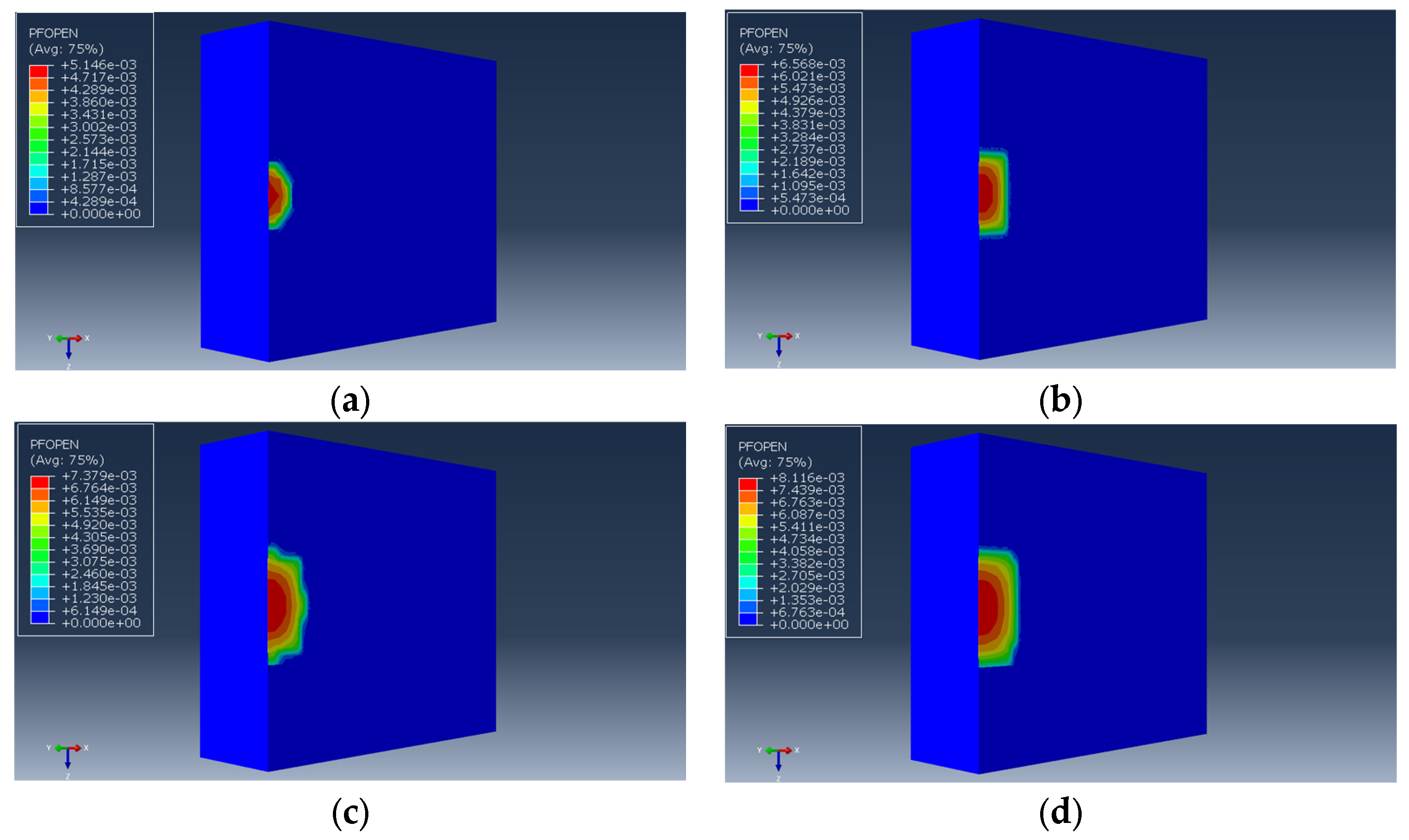
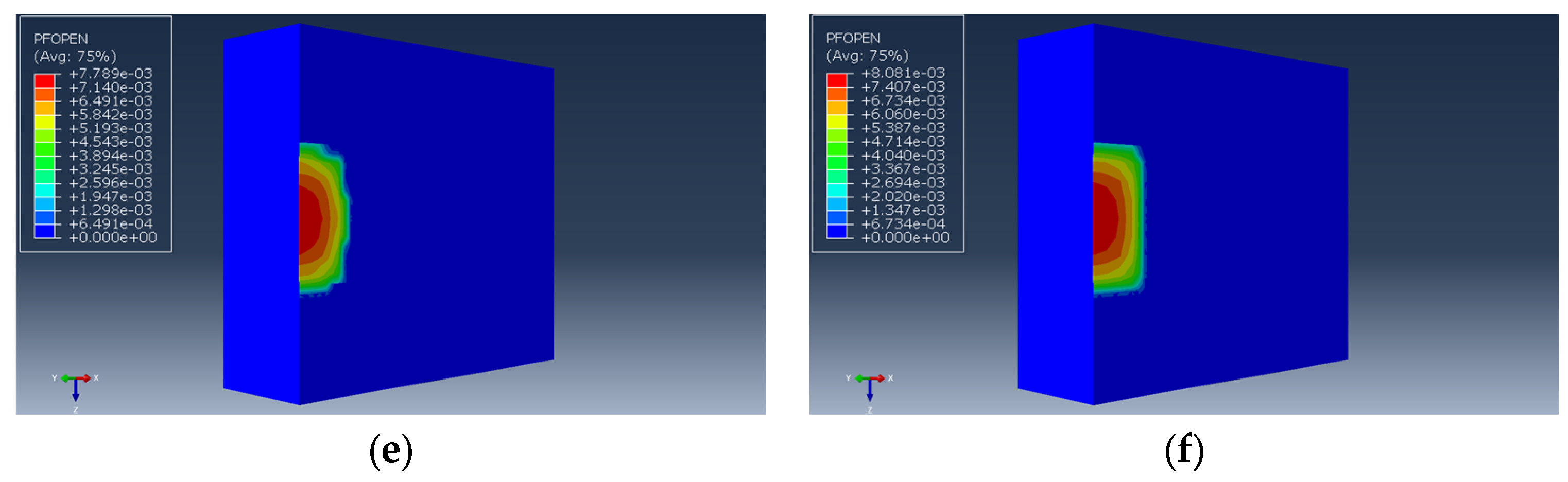
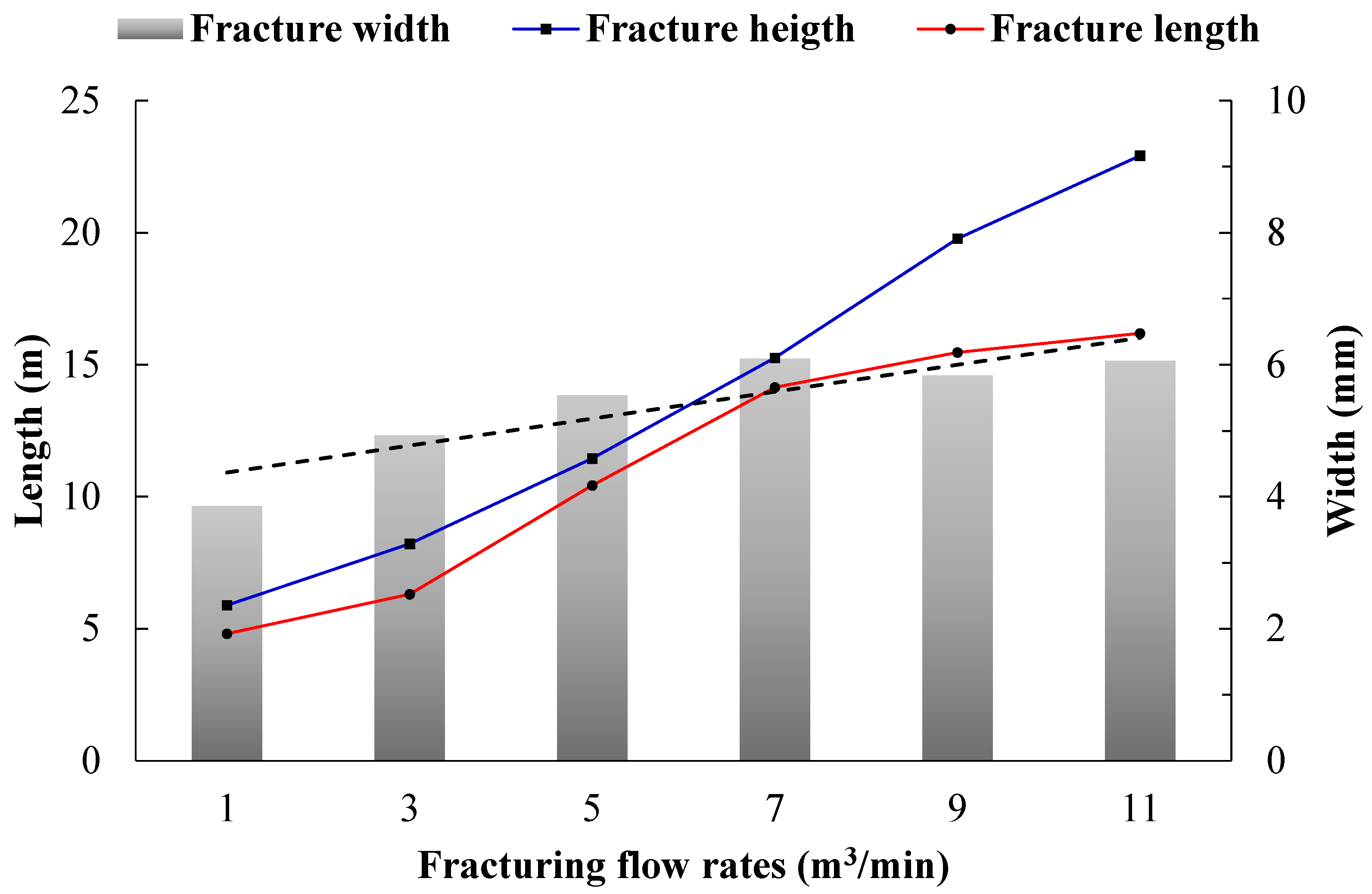
2.2.2. Engineering Construction Parameters Influence

The geological lithological factors explored in the previous section refer to the inherent properties of the formation and their uncontrollable influence on the vertical extension of hydraulic fractures. However, in hydraulic fracturing operations, the volume, displacement, and viscosity of fracturing fluid are controllable parameters. Clarifying the influence patterns of these key construction parameters on the vertical extension of hydraulic fractures is of greater significance for optimizing fracturing pump injection design and effectively controlling fracture height.

(1) Fracturing fluid flow rate

Due to the competition between fracture height and length during the initial stage of fracture propagation, further simulations were conducted to investigate the initial expansion of hydraulic fractures under different fracturing flow rates. The fracturing flow rates $Q$ were varied to 1, 3, 5, 7, 9, and 11 m³/min, studying their influence on the vertical expansion of hydraulic fractures during the initial stage. The morphology of fracture initial expansion and the corresponding results are illustrated in Figure 16 and Figure 17, respectively.

In Figure 17, it can be seen that with the increasing flow rate, the initial height, length, and average width of hydraulic fractures also increase continuously. When the flow rate is relatively low (between 1 and 7 m³/min), the growth rate of fracture height is slow while fracture length increases rapidly. However, when the flow rate is high (between 7 and 11 m³/min), the fracture height increases sharply with the flow rate, while the growth rate of fracture length significantly slows down. When the flow rate reaches 11 m³/min, the fracture height is approximately 2–4 times that of the low flow rate, indicating a significant impact of flow rate on the vertical expansion of hydraulic fractures. As shown in Figure 18, the fluid pressure within the fracture will increase significantly with the increase in displacement. Although the higher net pressure in the fracture promotes the fracture extension, it will also cause the fracture height to increase significantly.

(2) Fracturing fluid viscosity

Varying the viscosity of the fracturing fluid to 1, 10, 20, 50, 100, and 200 mPa∙s respectively, the influence of its impact on the vertical expansion of hydraulic fractures, the morphology of fracture expansion, and the calculation results are shown in Figure 19 and Figure 20.

In Figure 20, it can be seen that when the viscosity of the fracturing fluid varies from 1 to 100 mPa∙s, the height and length of the hydraulic fracture almost remain unchanged, while the average fracture width slightly increases as viscosity increases. However, when the viscosity of the fracturing fluid increases from 100 mPa∙s to 200 mPa∙s, the growth rate of fracture height significantly accelerates, while the fracture length decreases due to vertical expansion of the fracture. Analysis suggests that when the viscosity of the fracturing fluid increases to a certain extent, the filtration coefficient of the fracturing fluid becomes very low, leading to increasing frictional resistance as the fluid passes through the fracture, resulting in increased “backpressure” within the fracture, promoting vertical expansion of the fracture and increasing fracture height. Therefore, when using a gel-based fracturing fluid, attention should be paid to the potential issue of uncontrolled fracture height due to excessively high viscosity.

2.3. Orthogonal Analysis of Multi-Factor Vertical Expansion of Hydraulic Fractures

Combining typical geological mechanics of the Stone Box formation in the Linxing–Shinfu block and common construction parameters, orthogonal analysis was employed to further evaluate the influence of various factors on the vertical expansion of hydraulic fractures. Orthogonal simulation does not consider the interaction between multiple factors and adopts the L27 (38) scheme design. Details are presented in

Table 3. Orthogonal design table for the effect of fracture height.

	Factors	$\mathit{\Delta }{\mathit{\sigma }}_{\mathit{h}}$/MPa	$\mathit{h}$/m	$\mathit{\Delta }\mathit{E}$/GPa	$\mathit{\Delta }\mathit{\upsilon }$	$\mathit{\Delta }{\mathit{T}}_{\mathit{s}}$/MPa	$\mathit{V}$/m3	$\mathit{Q}$/m3∙min−1	$\mathit{\mu }$/mPa∙s
Levels
I		2	5	−2	0.02	2	250	3	20
II		4	10	−4	0.04	4	300	3.5	100
III		6	15	−6	0.06	6	350	4	200

.

Figure 21 shows the extreme difference in fracture height obtained from orthogonal analysis of various factors, reflecting the degree of influence of each factor on the vertical expansion of hydraulic fractures. Thus, under the geological and construction conditions of the Shihezi formation in the Linyi Sag, the influence of each factor on fracture height from strongest to weakest is as follows: stress difference between barrier/reservoir layers $\Delta {\sigma }_h$ > fracturing fluid viscosity $\mu$ > fracturing volume $Q$ > fracturing fluid volume $V$ > thickness of barrier layer $h$ > tensile strength difference between barrier/reservoir layers $\Delta T_s$ > elastic modulus difference between barrier/reservoir layers $\Delta E$ > Poisson’s ratio difference between barrier/reservoir layers $\Delta \upsilon$.

3. Prediction Study on Hydraulic Fracture Height

Based on the understanding of the vertical expansion pattern of hydraulic fractures, fracture height has a significant impact on the effectiveness of hydraulic fracturing. If it is possible to predict the fracture height of the target formation accurately, it allows for early identification of whether fractures will reach and communicate with adjacent strata posing risks. Subsequently, considering whether to employ fracture height control methods can effectively prevent remodeling failures caused by uncontrolled fracture heights.

Using the limit distance $\Delta H$ as the criterion for determining the height of hydraulic fractures is reasonable, as it reflects the degree of vertical expansion of hydraulic fractures. The specific definition may be as follows:

$$\Delta H={\displaystyle \frac{H-h}{2}}$$

(8)

The equation also includes H as the height of the supporting fracture, in meters, and h as the thickness of the reservoir, also in meters. For the typical geological mechanics and commonly used construction parameters in the real-field formation, a numerical model for predicting fracture height is established. It simulates the limit distance of fractures penetrating layers under different reservoir thicknesses (2 to 20 m), pumping rates (3 to 3.5 m³/min), and net fluid volumes (300 to 350 m³). The key parameters of the model are shown in

Table 4. Key parameters for numerical simulation of fracture height prediction in the Shihongzi formation of the Linxing–Shenfu block.

Parameter Categories	Parameter Name/Unit	Reservoir/Formation Parameters
Strata parameters	Thickness/m	2~20/20
	Porosity/%	7.8/2.4
	Permeability/mD	0.45/0.05
	Elastic modulus/GPa	29.8/22.6
	Poisson’s ratio	0.23/0.31
	Tensile strength/MPa	3.8/6.4
	Shear strength/MPa	32.3/46.7
	Fracture toughness/MPa∙m1/2	0.75
Pressure parameters	Interlaminar shear strength/MPa	1~7
Construction parameters	Net liquid volume/m3	300~350
	Displacement/m3∙min−1	3~3.5
	Fracturing fluid viscosity/mPa∙s	200

, and the fracture height prediction chart is illustrated in Figure 22.

Based on the above figure, a comparison is made between the predicted fracture heights of six fracturing wells and seven fracturing intervals with the actual post-fracturing microseismic monitoring fracture heights, as shown in

Table 5. Comparison between predicted and actual fracture heights of fracturing wells.

Well Number	Interlayer Stress DifferenceMPa	Reservoir Thickness m	Displacement m3/min	Net Liquid Volume m3	Predicted Fracture Height m	Actual Fracture Height m	Relative Error %
LX-A	1.35	14.0	3.5	356.4	44.9	40	12.3
LX-B	3.50	12.8	3.0	294.0	26.4	30	12.0
LX-C	1.70	20.4	3.5	289.7	26.8	30	10.7
LX-D	4.25	19.3	3.5	338.4	27.3	30	9.0
LX-E	2.96	21.7	3.5	294.6	27.6	30	8.0
LX-F	1.71	13.3	3.5	348.9	37.3	40	6.8
LX-G	2.00	10.0	3.0	304.8	35.1	30	17.0

. The comparison results indicate that the overall error in fracture height prediction ranges from 6.8% to 17.0%, with an average error of approximately 10.8%. The prediction reliability is relatively high, providing valuable reference for optimizing fracturing design.

4. Conclusions

Based on the numerical investigations of vertical expansion of hydraulic fractures and prediction method of fracture height for the tight gas reservoir, some key findings are as follows:

(1)

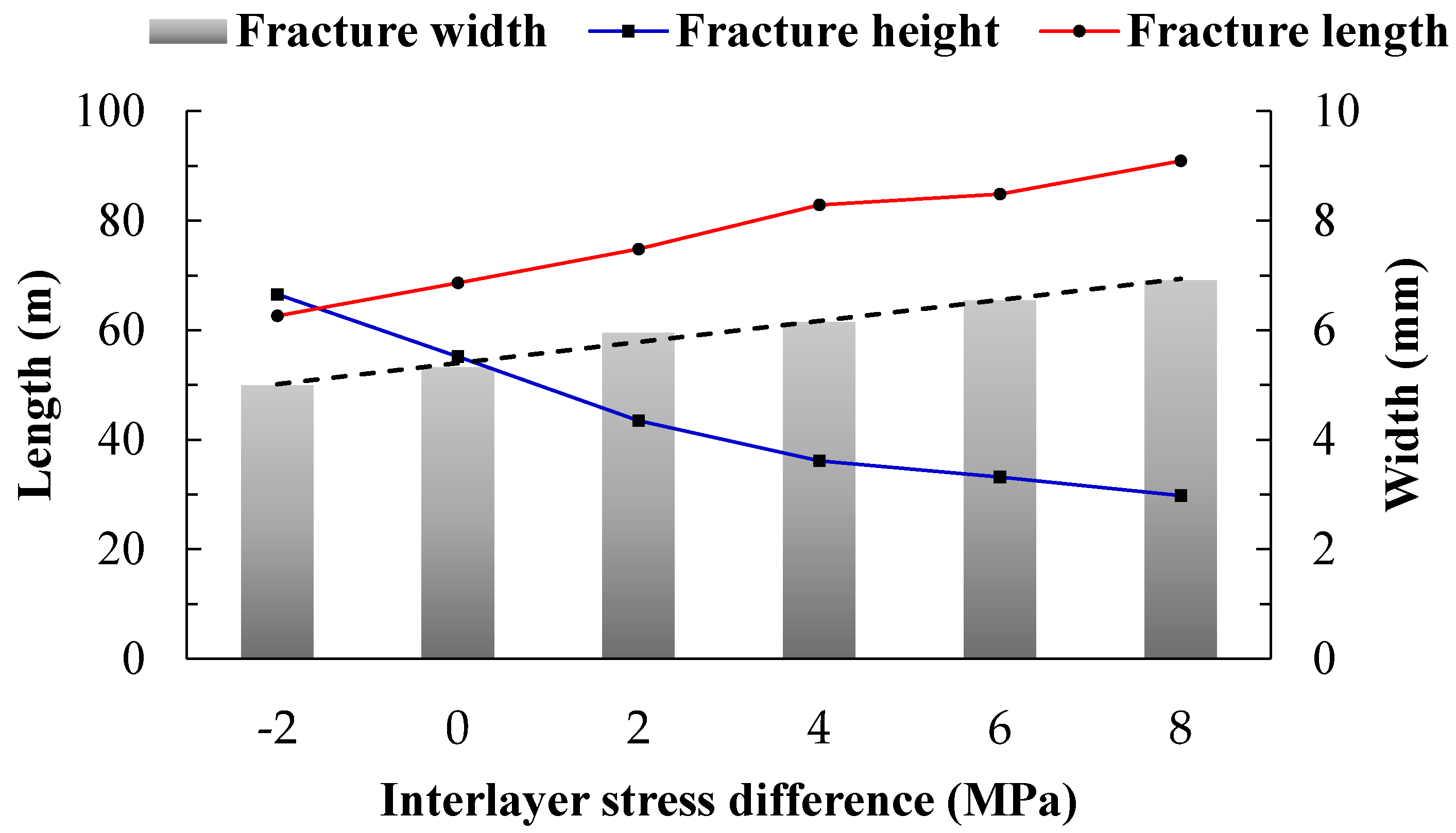
During the initial stage of fracture formation, there is a competition between vertical and horizontal propagation of hydraulic fractures. Once the initial shape of the fracture is determined, subsequent propagation of the fracture will more easily follow the direction of competitive advantage. Therefore, under the same conditions, the height and length of the fracture are inversely proportional, meaning that the smaller the fracture height, the greater the length of the fracture in the reservoir, and the larger the effective fracture volume;

(2)

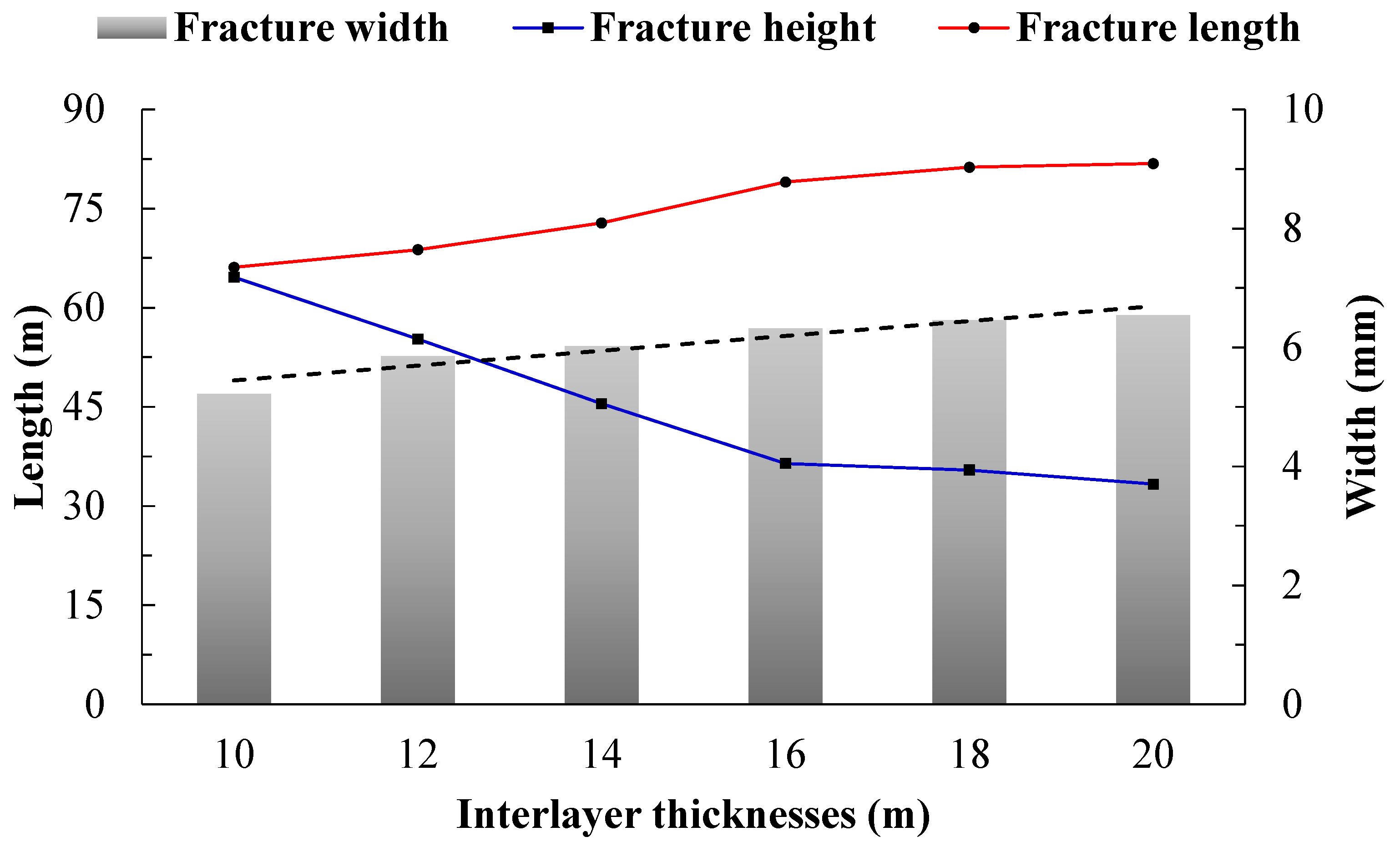
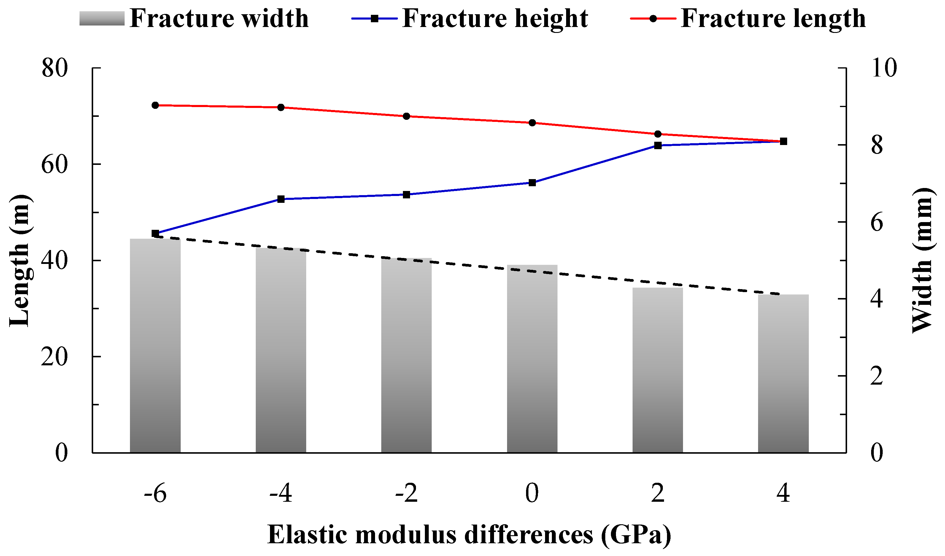
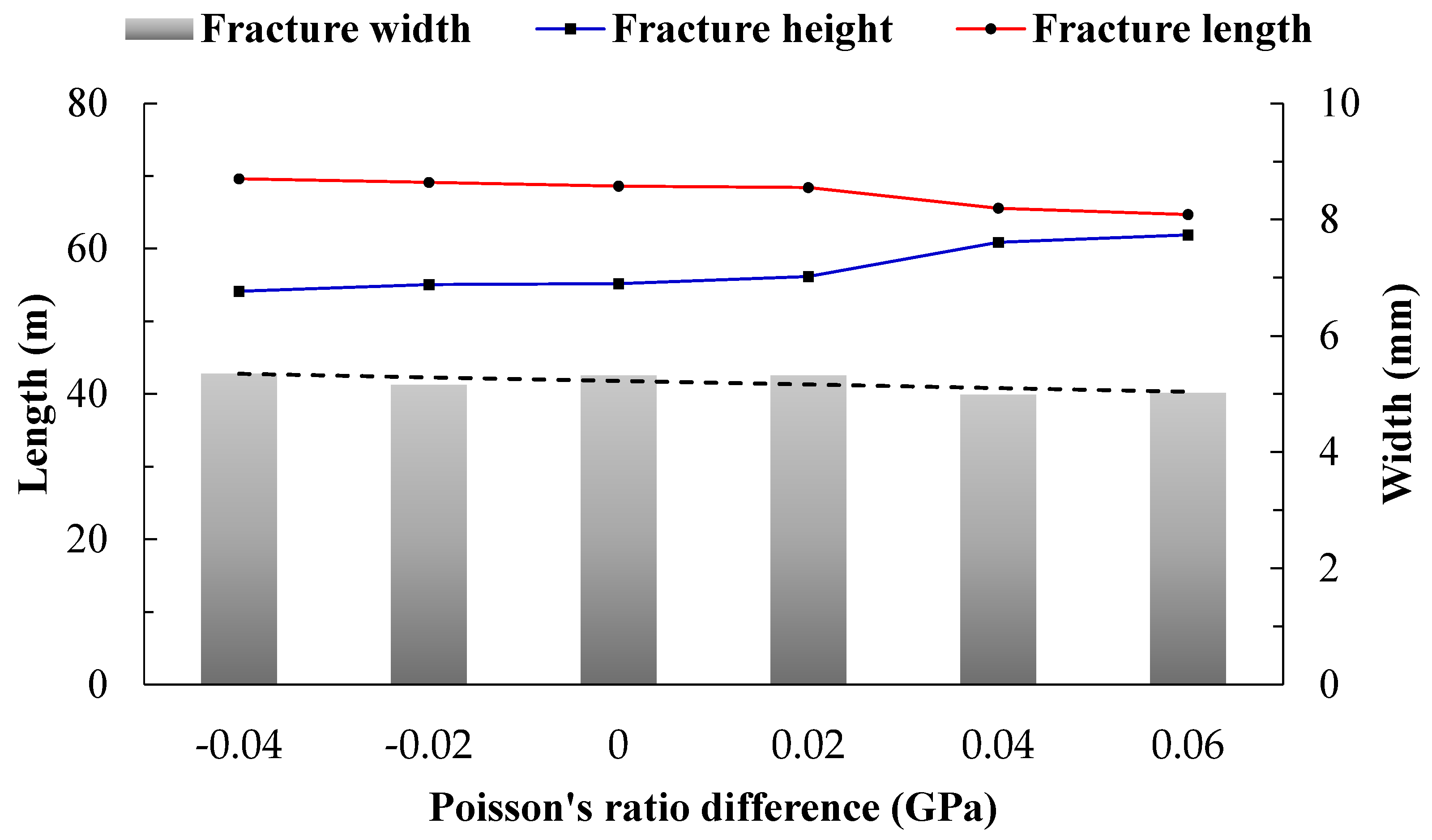
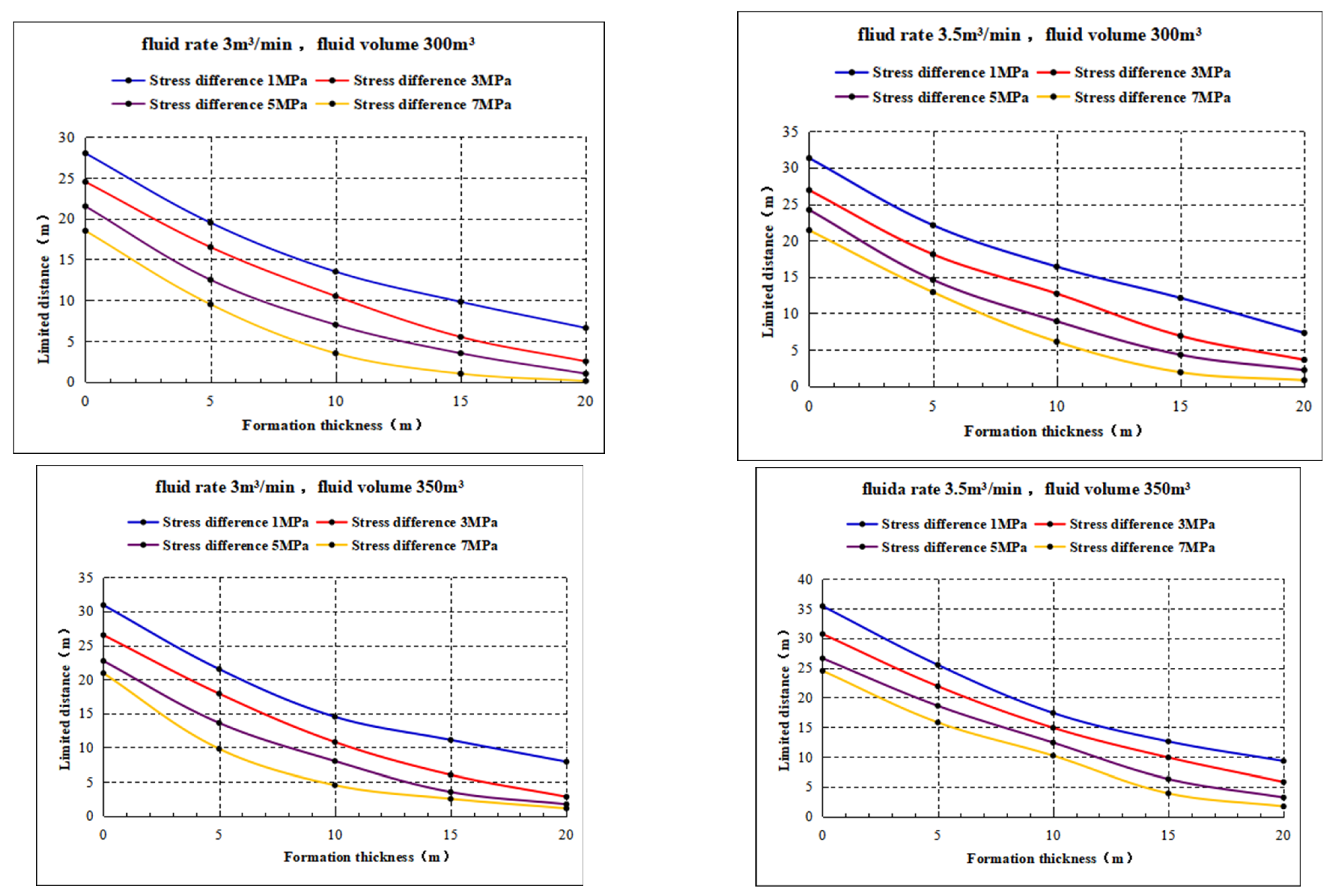
For geological lithological factors, the height of hydraulic fractures decreases with increasing thickness of interlayers, difference in stress between interlayers and reservoirs, difference in tensile strength, and difference in fracture toughness, while it increases with increasing difference in elastic modulus between interlayers and reservoirs. The influence of the difference in Poisson’s ratio between interlayers and reservoirs is not significant. Among these factors, the thickness of interlayers and the difference in stress and tensile strength between interlayers and reservoirs have a greater impact on fracture height. Compared to reservoirs, thicker interlayers with higher stress and tensile strength are more conducive to controlling fracture height;

(3)

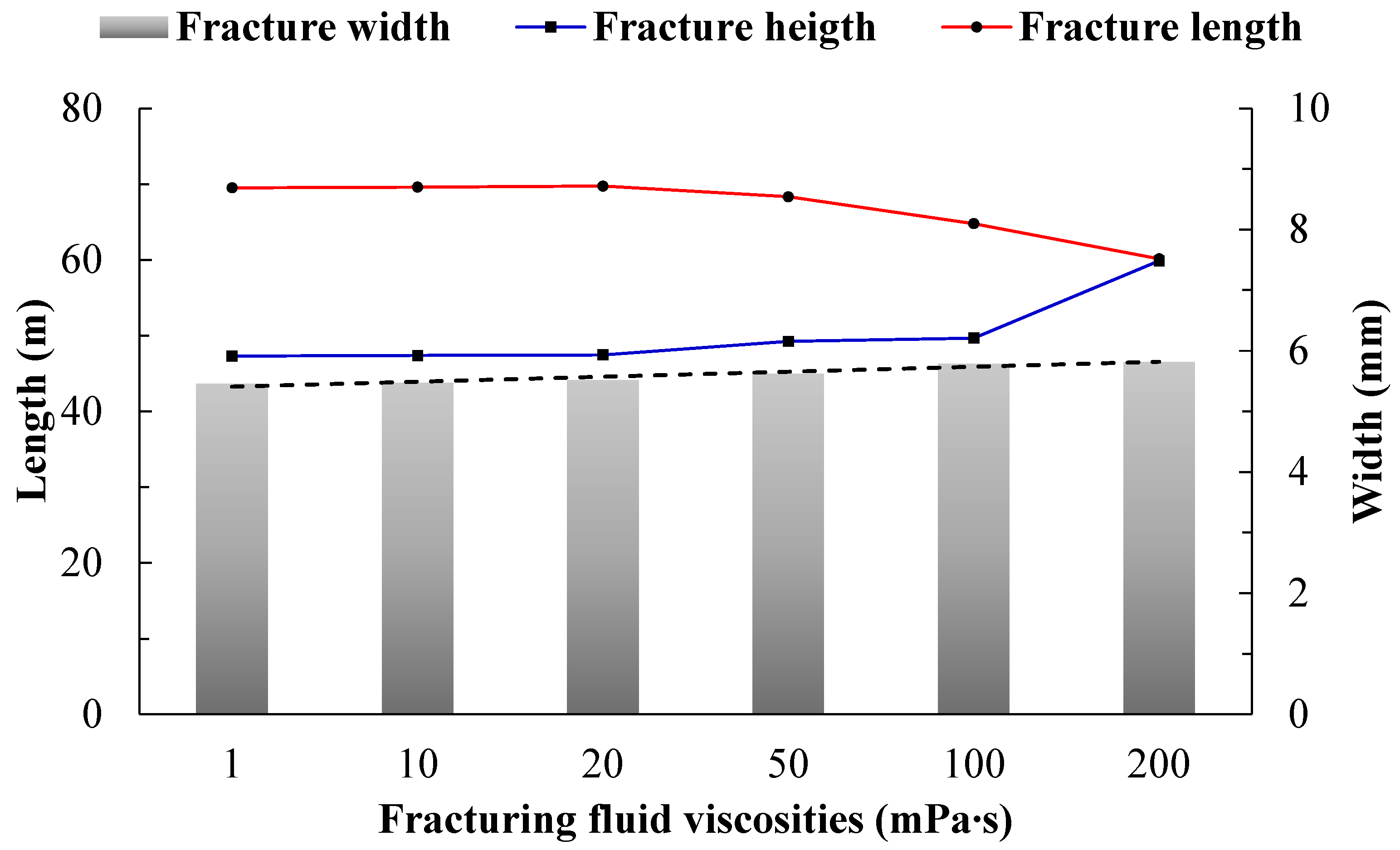
Regarding engineering construction parameters, the height of hydraulic fractures increases with increasing volume, rate, and viscosity of fracturing fluid. Among these factors, rate and viscosity have a greater impact on the initial vertical propagation of hydraulic fractures. A low rate and low viscosity during fracturing are conducive to promoting the longitudinal extension and propagation of hydraulic fractures, thereby avoiding uncontrolled increases in fracture height;

(4)

For the development of tight gas hydraulic fracturing in the Linxing–Shifu shale formation, the factors affecting fracture height are in the following order: stress difference between interlayers and reservoirs > fracturing fluid viscosity > fracturing rate > fracturing fluid volume > thickness of interlayers > difference in tensile strength between interlayers and reservoirs > difference in elastic modulus between interlayers and reservoirs > difference in Poisson’s ratio between interlayers and reservoirs;

(5)

A preliminary prediction chart for fracture height in the Linxing–Shifu shale formation has been established, with an average prediction error of about 10.8%. The reliability is relatively high, providing some guidance for optimizing fracturing design in the area.

References

1. Naceur, K.B.; Touboul, E. Mechanisms Controlling Fracture-Height Growth in Layered Media. SPE Prod. Eng. 1990, 5, 142–150. [Google Scholar] [CrossRef]
2. Simonson, E.R.; Abou-Sayed, A.S.; Clifton, R.J. Containment of massive hydraulic fractures. Soc. Pet. Eng. J. 1978, 18, 27–32. [Google Scholar] [CrossRef]
3. Huang, L.; Dontsov, E.; Fu, H.; Lei, Y.; Weng, D.; Zhang, F. Hydraulic fracture height growth in layered rocks: Perspective from DEM simulation of different propagation regimes. Int. J. Solids Struct. 2022, 238, 111395. [Google Scholar] [CrossRef]
4. Warpinski, N.R.; Schmidt, R.A.; Northrop, D.A. In-situ stresses: The predominant influence on hydraulic fracture containment. J. Pet. Technol. 1982, 34, 653–664. [Google Scholar] [CrossRef]
5. Gu, H.; Siebrits, E. Effect of Formation Modulus Contrast on Hydraulic Fracture Height Containment. SPE Prod. Oper. 2008, 23, 170–176. [Google Scholar] [CrossRef]
6. Gu, H.; Siebrits, E.; Sabourov, A. Hydraulic fracture modeling with bedding plane interfacial slip. In Proceedings of the SPE Eastern Regional/AAPG Eastern Section Joint Meeting, Pittsburgh, PA, USA, 11–15 October 2008. Society of Petroleum Engineers. [Google Scholar]
7. Eekelen, V. Hydraulic Fracture Geometry: Fracture Containment in Layered Formations. Soc. Pet. Eng. J. 1982, 22, 341–349. [Google Scholar] [CrossRef]
8. Smith, M.B.; Bale, A.B.; Britt, L.K.; Klein, H.H.; Siebrits, E.; Dang, X. Layered Modulus Effects on Fracture Propagation, Proppant Placement, and Fracture Modeling. In Proceedings of the SPE Annual Technical Conference and Exhibition, Denver, CO, USA, 30 October–2 November 2011. Society of Petroleum Engineers. [Google Scholar]
9. Huang, J.; Morris, J.P.; Fu, P.; Settgast, R.R.; Sherman, C.S.; Ryerson, F.J. Hydraulic-fracture-height growth under the combined influence of stress barriers and natural fractures. SPE J. 2019, 24, 302–318. [Google Scholar] [CrossRef]
10. Salah, M.; Gabry, M.A.; ElSebaee, M.; Mohamed, N. Control of hydraulic fracture height growth above water zone by inducing artificial barrier in Western Desert, Egypt. In Proceedings of the Abu Dhabi International Petroleum Exhibition and Conference, Abu Dhabi, United Arab Emirates, 7–10 November 2016. Society of Petroleum Engineers. [Google Scholar]
11. Li, J.; Wu, K. An efficient model for hydraulic fracture height growth considering the effect of bedding layers in unconventional shale formations. SPE J. 2022, 27, 3740–3756. [Google Scholar] [CrossRef]
12. Gao, Q.; Ghassemi, A. Three dimensional finite element simulations of hydraulic fracture height growth in layered formations using a coupled hydro-mechanical model. Int. J. Rock Mech. Min. Sci. 2020, 125, 104137. [Google Scholar] [CrossRef]
13. Detounay, E. Propagation regimes of fluid-driven fractures in impermeable rocks. Int. J. Geomech. 2004, 4, 35–45. [Google Scholar] [CrossRef]
14. Chen, Z.X.; Chen, M.; Huang, R.Z.; Shen, Z.H. Vertical propagation of hydraulic fractures in layered formation. J. China Univ. Pet. (Ed. Nat. Sci.) 1997, 21, 23–26, 32. [Google Scholar]
15. Qin, M.; Yang, D. Numerical investigation of hydraulic fracture height growth in layered rock based on peridynamics. Theor. Appl. Fract. Mech. 2023, 125, 103885. [Google Scholar] [CrossRef]
16. Cong, Z.; Li, Y.; Tang, J.; Martyushev, D.A.; Yang, F. Numerical simulation of hydraulic fracture height layer-through propagation based on three-dimensional lattice method. Eng. Fract. Mech. 2022, 264, 108331. [Google Scholar] [CrossRef]
17. Tang, J.; Wu, K. A 3-D model for simulation of weak interface slippage for fracture height containment in shale reservoirs. Int. J. Solids Struct. 2018, 144, 248–264. [Google Scholar] [CrossRef]
18. Kresse, O.; Weng, X.; Mohammadnejad, T. Modeling the effect of fracture interference on fracture height growth by coupling 3D displacement discontinuity method in hydraulic fracture simulator. In ARMA US Rock Mechanics/Geomechanics Symposium; ARMA: San Francisco, CA, USA, 2017; p. ARMA–2017. [Google Scholar]
19. Mehrabi, M.; Pei, Y.; Haddad, M.; Javadpour, F.; Sepehrnoori, K. Quasi-static fracture height growth in laminated reservoirs: Impacts of stress and toughness barriers, horizontal well landing depth, and fracturing fluid density. In Proceedings of the Unconventional Resources Technology Conference (URTeC), Houston, TX, USA, 26–28 July 2021; pp. 1027–1046. [Google Scholar]
20. Rho, S.; Noynaert, S.; Bunger, A.P.; Zolfaghari, N.; Xing, P.; Abell, B.; Suarez-Rivera, R. Finite-element simulations of hydraulic fracture height growth on layered mudstones with weak interfaces. In ARMA US Rock Mechanics/Geomechanics Symposium; ARMA: San Francisco, CA, USA, 2017; p. ARMA–2017. [Google Scholar]
21. Yang, L.; Chen, B. Extended finite element-based cohesive zone method for modeling simultaneous hydraulic fracture height growth in layered reservoirs. J. Rock Mech. Geotech. Eng. 2024. [Google Scholar] [CrossRef]
22. Du, J.; Chen, X.; Liu, P.; Zhao, L.; Chen, Z.; Yang, J.; Chen, W.; Wang, G.; Lou, F.; Miao, W. Numerical Modeling of Fracture Height Propagation in Multilayer Formations Considering the Plastic Zone and Induced Stress. ACS Omega 2022, 7, 17868–17880. [Google Scholar] [CrossRef] [PubMed]
23. Li, H.; Zou, Y.; Valko, P.P.; Ehlig-Economides, C. Hydraulic fracture height predictions in laminated shale formations using finite element discrete element method. In Proceedings of the SPE Hydraulic Fracturing Technology Conference and Exhibition, Woodlands, TX, USA, 9–11 February 2016; SPE: The Woodlands, TX, USA, 2016; p. D011S001R002. [Google Scholar]
Figure 1. Bilinear traction–separation constitutive model of cohesive element.
Energies 17 03785 g001
Figure 2. The fluid flow schematic within the cohesive zone.
Energies 17 03785 g002
Figure 3. Calculation results of typical rock physical parameters of Shihezi formation based on the logging data of fractured wells in the target block. None represents the gas free layer, Medium represents the medium gas containing layer, Good represents the gas rich layer, and belongs to the high-quality gas layer.
Energies 17 03785 g003
Figure 4. Calculation results of typical rock mechanical parameters of Shihezi formation based on the logging data of fractured wells in the target block.
Energies 17 03785 g004
Figure 5. Depiction of a schematic diagram of the three-dimensional layered finite element computational model. (a) Model geometry, (b) Model grid division.
Energies 17 03785 g005
Figure 6. Hydraulic fracture morphology under different interlayer stress differences between shale interlayers and reservoir layers. (a) Δ σ h = 2   MPa , (b) Δ σ h = 0   MPa , (c) Δ σ h = 2   MPa , (d) Δ σ h = 4   MPa , (e) Δ σ h = 6   MPa , (f) Δ σ h = 8   MPa .
Energies 17 03785 g006aEnergies 17 03785 g006b
Figure 7. Hydraulic fracture calculation results under different interlayer stress differences between shale interlayers and reservoir layers.
Energies 17 03785 g007
Figure 8. Hydraulic fracture morphology under different reservoir thicknesses. (a) h = 10   m , (b) h = 12   m , (c) h = 14   m , (d) h = 16   m , (e) h = 18   m , (f) h = 20   m .
Energies 17 03785 g008
Figure 9. Presentation of the calculation results of hydraulic fractures under different interlayer thicknesses.
Energies 17 03785 g009
Figure 10. Hydraulic fracture morphology under different barrier/storage layer elastic modulus differences. (a) Δ E = 6   GPa , (b) Δ E = 4   GPa , (c) Δ E = 2   GPa , (d) Δ E = 0   GPa , (e) Δ E = 2   GPa , (f) Δ E = 4   GPa .
Energies 17 03785 g010aEnergies 17 03785 g010b
Figure 11. Hydraulic fracture calculation results under different barrier/storage layer elastic modulus differences.
Energies 17 03785 g011
Figure 12. Illustration of the morphology of hydraulic fractures under different contrasts in Poisson’s ratio between the barrier and reservoir layers. (a) Δ υ = 0.04 , (b) Δ υ = 0.02 , (c) Δ υ = 0 , (d) Δ υ = 0.02 , (e) Δ υ = 0.04 , (f) Δ υ = 0.06 .
Energies 17 03785 g012
Figure 13. Display of the computed results of hydraulic fractures under different contrasts in Poisson’s ratio between the barrier and reservoir layers.
Energies 17 03785 g013
Figure 14. Hydraulic fracture morphology under different differences in tensile strength between barrier and reservoir formations. (a) Δ T s = 2   MPa , (b) Δ T s = 1   MPa , (c) Δ T s = 0   MPa , (d) Δ T s = 1   MPa , (e) Δ T s = 2   MPa , (f) Δ T s = 3   MPa .
Energies 17 03785 g014aEnergies 17 03785 g014b
Figure 15. Calculation results of hydraulic fractures under different differences in tensile strength between barrier and reservoir formations.
Energies 17 03785 g015
Figure 16. Illustration of the initial morphology of hydraulic fractures under various fracturing flow rates. (a) Q = 1   m 3 / min , (b) Q = 3   m 3 / min , (c) Q = 5   m 3 / min , (d) Q = 7   m 3 / min , (e) Q = 9   m 3 / min , (f) Q = 11   m 3 / min .
Energies 17 03785 g016aEnergies 17 03785 g016b
Figure 17. Initial calculation results of hydraulic fractures under different fracturing flow rates.
Energies 17 03785 g017
Figure 18. Calculation results of injection point pressure under different fracturing displacement.
Energies 17 03785 g018
Figure 19. Hydraulic fracture morphology under different fracturing fluid viscosities. (a) μ = 1   mP · s , (b) μ = 10   mP · s , (c) μ = 20   mP · s , (d) μ = 50   mP · s , (e) μ = 100   mP · s , (f) μ = 200   mP · s .
Energies 17 03785 g019
Figure 20. Calculation results of hydraulic fractures under different fracturing fluid viscosities.
Energies 17 03785 g020
Figure 21. Simulation results of extreme difference in fracture height from multi-factor orthogonal analysis.
Energies 17 03785 g021
Figure 22. Predicted height of fracture in the Lingshenfu Stone Box group fracturing.
Energies 17 03785 g022