Abstract
Sail-assisted propulsion is an important energy-saving technology in the shipping industry, and the development of foldable wingsails has recently become a hot topic. This type of sail is usually composed of multiple elements, and its performance at different folding configurations is very sensitive to changes in incoming airflow, which result in practical operational challenges. Therefore, original and optimized three-element wingsails (bare and concave) are modeled and simulated using the unsteady RANS method with the k-ω SST turbulence model. Next, certain key design and structural parameters (such as angle of attack, apparent wind angle, and camber) are employed to characterize the auxiliary propulsion performance, and the differences are explained in combination with the flow field details. The results show that, in the unfolded state, the aerodynamic performance of the concave wingsail is better than that of the bare wingsail, exhibiting higher lift coefficients, lower drag coefficients, and a more stable surface flow. In the fully folded state, wherein both the nose and flap are rotated, the thrust performance of the concave wingsail remains superior. Specifically, at an angle of attack of 8 degrees, the thrust coefficient of the concave wingsail is approximately 23.5% higher than that of the bare wingsail, indicating improved wind energy utilization. The research results are of great significance for engineering applications and subsequent optimization design.
1. Introduction
In April 2018, the International Maritime Organization (IMO) adopted the initial strategy for Greenhouse Gas (GHG) emissions, establishing targets and measures to reduce GHG emissions from international shipping [1]. In July 2023, during the 80th session of the Marine Environment Protection Committee (MEPC 80), the initial GHG strategy underwent its first revision, aiming to curb GHG emissions from vessels. The revised strategy set new targets, including a 20% emission reduction by 2030, a 70% reduction by 2040 (relative to 2008 levels), and achieving net-zero emissions by 2050 [2]. Within this context, wingsail-assisted propulsion technology received widespread attention in the shipping and shipbuilding industries for its environmentally friendly and sustainable advantages. This technology utilizes renewable wind energy, decreasing fuel consumption without generating additional onboard carbon emissions [3,4]. As sustainability objectives in shipping intensify, further research into innovative wingsail designs may enable greater adoption of this clean propulsion solution.
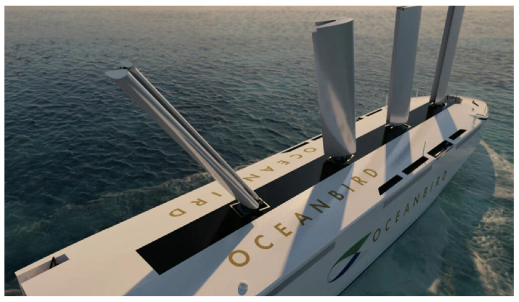
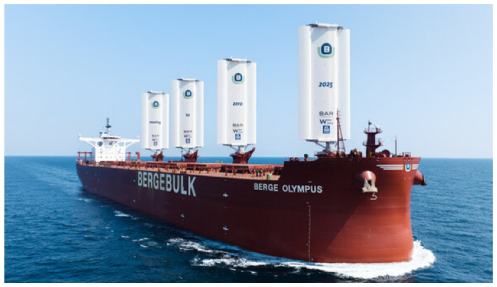
In recent years, the development of wingsail-assisted propulsion technology has gradually begun to consider the folding property in both commercial applications and academic research. In August 2023, the foldable two-element wingsail “Wing 560” (Figure 1), designed by Oceanbird, received Approval in Principle (AiP) from the classification society DNV [5]. The wingsail has a height of 40 m, a width of 14 m, and a total sail area of 560 square meters. It consists of two elements, the main body and the flap, and can optimize aerodynamic forces by creating camber profiles. As for the performance, one wingsail on an existing RoRo vessel at normal speed can reduce fuel consumption from the main engine by 7–10% on favorable oceangoing routes. This means a saving of 600 tons of diesel per year, which corresponds to approx. 1920 tons of CO2. In October 2023, a bulker was equipped with four foldable three-element wingsails, “WindWings” (Figure 2), which was designed by BARTech, aiming to use wind power to reduce fuel consumption and CO2 emissions [6]. Each of the four “WindWings” measures 20 m in width and 37.5 m in height, and the total surface area of the four wings is 3000 square meters. It consists of three elements, the nose, the main body, and the flap, and can also create cambers by rotating the nose and flap. As for the performance, the “WindWings” can save up to 20% fuel, reducing CO2 emissions by 19.5 tons per day on an average worldwide route. The similarity between the “Wing 560” and “WindWings” is that both can form different folding configurations through camber angles, thereby fully utilizing the auxiliary performance. However, the performance is very sensitive to the incoming airflow, resulting in difficulties in practical operations; therefore, research on such issues is necessary.

Figure 1.
A RoRo vessel with “Wing 560”.
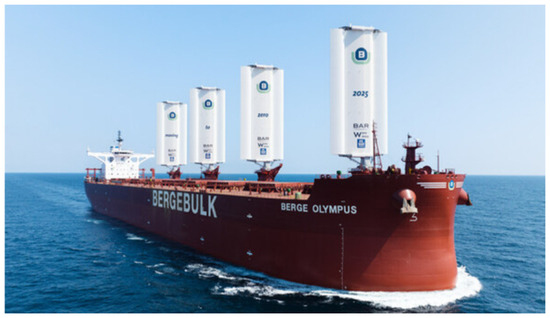
Figure 2.
A bulker with “WindWings”.
Currently, two main approaches are used for studying foldable wingsail performance: model tests and numerical simulations. In 2015, Furukawa [7] conducted a model test to measure the effect of gap geometry, angle of attack, and camber on the performance characteristic of a two-element wingsail, which consists of two different symmetrical airfoils (NACA0025, NACA0009). The gap size and pivot point of the rear element were found to have only a weak influence on the lift and drag coefficients, while increasing the camber can effectively increase the lift coefficient. However, too high a camber will lead to a certain increase in drag.
With advances in computer technology, wingsail performance can be studied using CFD simulation tools, offering a low-cost solution in terms of time and equipment compared to model tests [8]. In 2020, Li [9] conducted a comparative numerical study of a two-element wingsail using steady and unsteady Reynolds-Averaged Navier–Stokes (RANS) methods. The analysis included an examination of the aerodynamic performance at different bends, flap rotational axis positions, angles of attack, and flap thicknesses, ultimately revealing the nonlinear coupling effect between the bends and flap rotational axis positions. In 2023, Li [10] numerically investigated the aerodynamic performance of a two-element wingsail under gradient and uniform winds, discovering that the gradient wind condition could delay instances of stalling.
However, most previous experimental and numerical simulations have been conducted on two-element wingsails, and very little information is available in the open peer-reviewed literature of foldable three-element wingsails. In comparison, the folding configuration of the three-element wingsail is more complex when considering the cambers of sub-wings. Therefore, an original three-element wingsail will be modeled, and the design will be further optimized to further improve the efficiency of wind energy utilization. Firstly, the aerodynamic and thrust performance of wingsails in the unfolded state will be studied, and the effects of AOA and the apparent wind angle on the lift, drag, and thrust coefficients will be evaluated. Then, considering the foldable properties of wingsails, the thrust performance will be evaluated for a single rotation of the nose and flap separately. Finally, both the nose and flap will be rotated to find the target folding configuration that produces the maximum thrust coefficient. Furthermore, aerodynamic and thrust performance results will be comprehensively analyzed by considering corresponding flow detail characteristics.
2. Model and Methods
2.1. Geometry
Referring to the cross-section of the “WindWings” described in the Introduction, the bare three-element wingsail is first modeled, and the geometry is obtained by stretching three NACA0012 airfoil profiles, as shown in Figure 3a. In addition, with reference to the “slotted flap” design of a two-element sail introduced by Blakeley [11], the airfoil profile of the bare three-element wingsail is optimized, resulting in a concave three-element wingsail, as shown in Figure 3b. Although this wingsail also consists of three parts, as a whole, it has the same shape as the single airfoil pattern. It should be noted that the cross-section type of both the bare and concave three-element wingsail is further designed based on the NACA0012 airfoil profile, and a detailed description of the configuration and parameters will be carried out in the following content.
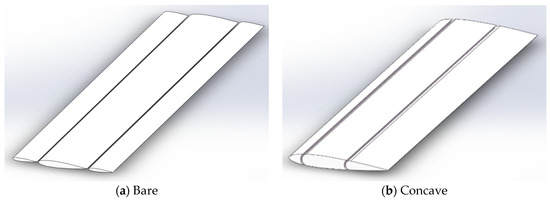
Figure 3.
Three-dimensional model of the wingsails.
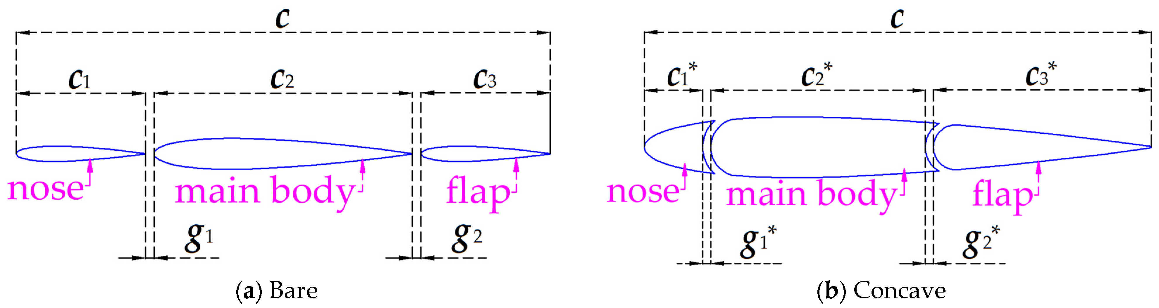
As shown in Figure 4, both the bare and concave three-element wingsails consist of three parts—a nose, main body, and flap—with their specific dimensional parameters detailed in Table 1. To ensure a consistent variable for the comparative study, the total chord length (c) of each wingsail is set to 1 m. The nose, main body, and flap have chord length ratios of 1:2:1 for the bare design and 1:3.7:3.7 for the concave design. In addition, gaps are present between neighboring portions of the wingsails. To mitigate the impact of gap size on the study results, all gap sizes are set to be the same. It should be noted that both the nose and flap of the bare and concave wingsails can be rotated at an angle to create different cambers, resulting in different folding configurations, which will be described in Section 3.2.
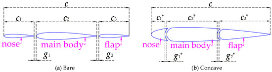
Figure 4.
Parameterization of the wingsails.

Table 1.
Parameterization of the wingsails.
2.2. Force Analysis of Wingsail
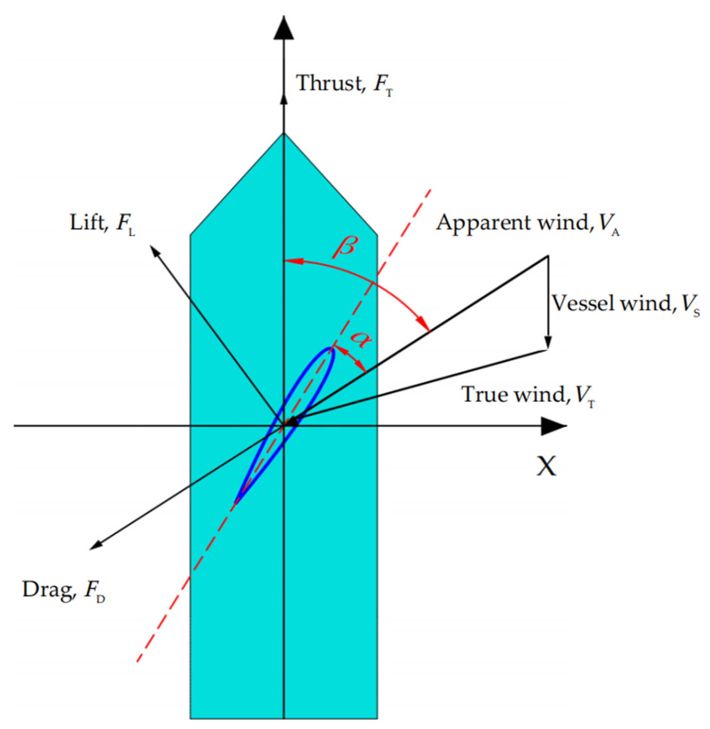
A wingsail is a rigid sail, similar to a wing, that utilizes the Bernoulli effect to generate aerodynamic forces. The airfoil profile allows airflow to pass through, creating a velocity difference, which in turn generates a pressure difference, i.e., lift. This lift, along with the friction component in the direction of sailing, constitutes the propulsive force (as shown in Figure 5). When a vessel is sailing, the wind acting on the surface of the wingsails consists of three components: apparent wind, true wind, and vessel wind. The direction of vessel wind is opposite to the vessel’s sailing direction, and the apparent wind is obtained by synthesizing the true wind and vessel wind vectors. The thrust can be determined by synthesizing the lift and drag components in the heading direction, where is the angle of attack (AOA), is the apparent wind angle (AWA), is the true wind speed (TWS), is the apparent wind speed (AWS), and is the wind speed caused by vessel sailing.
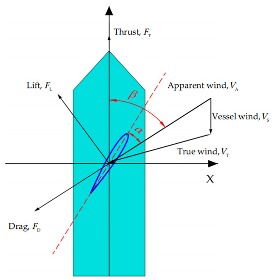
Figure 5.
Wind triangle and loads on the wingsail.
Focusing on thrust coefficients provides a more directly applicable perspective compared with individual lift and drag values when evaluating wingsail performance for maritime propulsion [12]. Based on the lift and drag coefficients (as shown in Equations (1) and (2)), the thrust coefficient can be calculated by incorporating the apparent wind angle (as shown in Equation (3)). Here, represents the density of air and denotes AWS. The reference area in the lift and drag coefficients can be replaced by the total chord length of the wingsail in a two-dimensional study [13].
2.3. Numerical Setup
2.3.1. Computational Domain
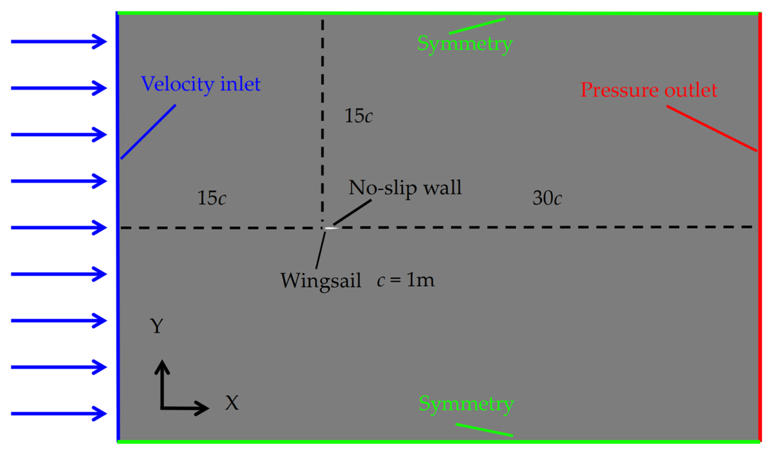
Subsequent numerical simulations are conducted using Star CCM+, a CFD calculation program developed based on the finite volume method (FVM) [14]. In this simulation program, appropriately generating the mesh and configuring the boundary layer settings are critical prerequisites. As depicted in Figure 6, a two-dimensional rectangular fluid computational domain is established with a length of 45 c and width of 30 c. The top and bottom boundaries are symmetric planes aimed at minimizing sidewall effects, while the right side serves as a pressure outlet. Additionally, the sail surface is modeled as a fixed no-slip wall.

Figure 6.
Dimensions of the computational domain and boundary conditions.
Choosing an appropriate turbulence model is equally important when solving the flow field around the wingsail. Hassan [15] used standard, RNG, and realizable models and standard and SST models to simulate the aerodynamic performance of an NACA0018 airfoil; compared it with experimental results; and found that the SST model can achieve more accurate predictions. In STAR-CCM+, the SST model is a turbulence model that is used alongside a RANS simulation. This model shares similarities with the model, with the main difference being that the SST model uses a hybrid approach. If the cells are close to the wall, the model will be applied, and if the cells are far away in the free stream, then the model will be applied.
2.3.2. Mesh Generation and Convergence Test
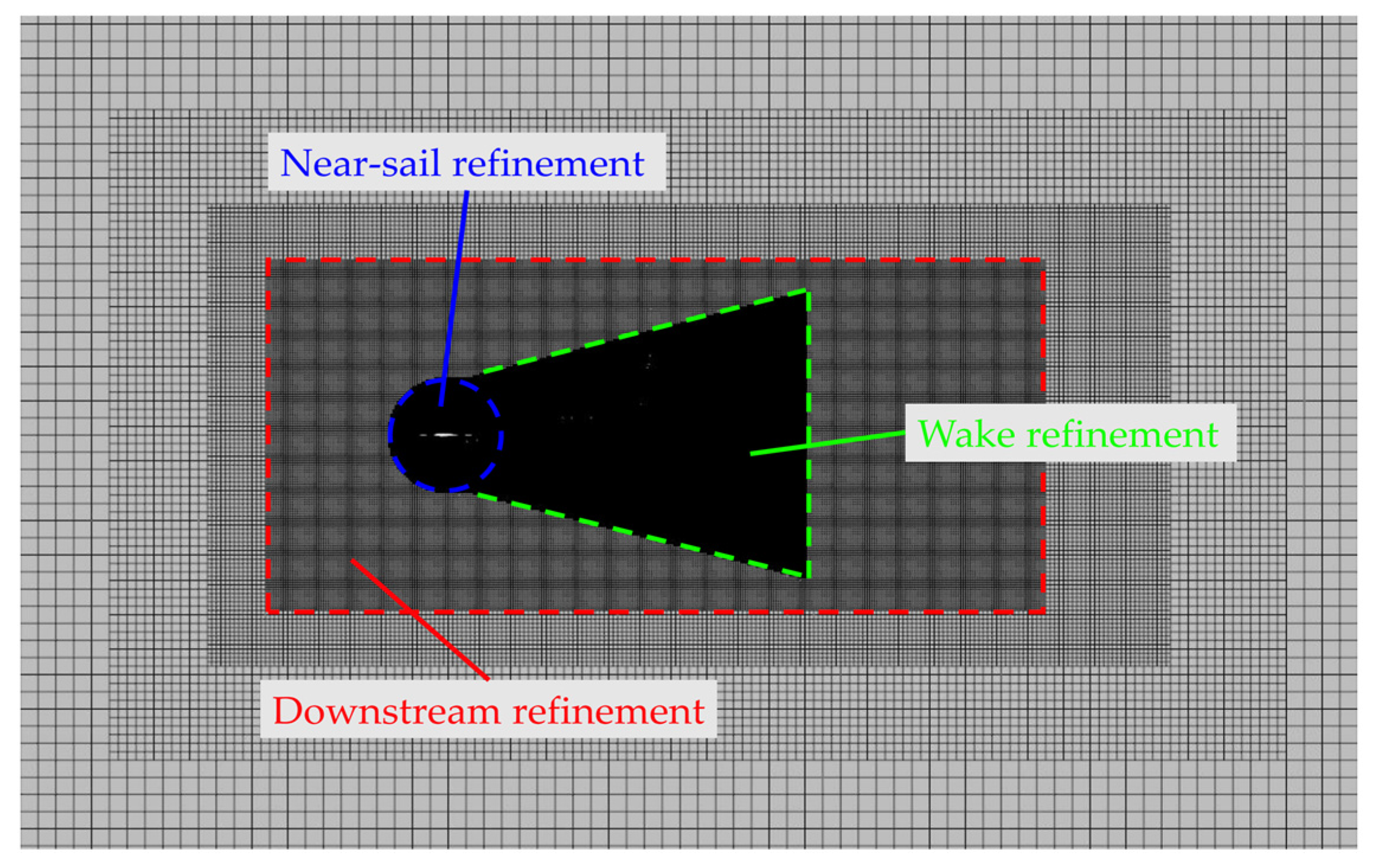
In STAR-CCM+, three meshers (Surface Remesher, Trimmed Cell Mesher, and Prism Mesher) are used to generate meshes, and the meshes for the near-sail, wake, and downstream regions are refined separately. The circular and trapezoidal zones near the wingsail allow flow detail features to be effectively captured. In addition, by adjusting various mesh parameters (including the base size, the relative target size, the minimum surface size, the number, and the thickness of prism layers), the final mesh structure is obtained, as shown in Figure 7.
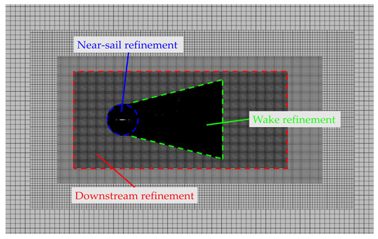
Figure 7.
A view of the computational mesh showing refined areas around the geometry.
In the aerodynamic simulation of a wingsail, the meshes of the boundary layer have a significant influence on the results. This layer helps the solver to accurately resolve the flow near the wall, which is vital for determining forces or other flow features, such as separation [16]. Therefore, the prism layer mesher is used to generate the boundary layer. The number of layers is set to 20, the prism layer thickness is set to 0.01 m, and the thickness of the first layer is set to 1.0 × 10⁻⁵ m (as shown in Figure 8). As shown in Figure 9, the mean value of Y+ values for both bare and concave three-element wingsail surfaces is less than 1, proving that the boundary layer meshes meet the requirement of simulation accuracy.
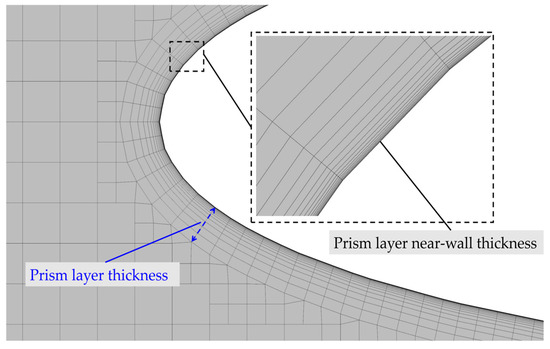
Figure 8.
Prism layer close to geometry curves.
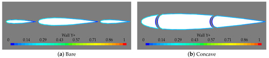
Figure 9.
Wall Y+ distribution around two types of three-element wingsails.
In order to accurately capture the time-dependent flow simulation, the Courant–Friedrichs–Lewy (CFL) is introduced (as Equation (4)), where is the velocity of the fluid, is the time step, and is the characteristic length of the mesh. Referring to the study of Li [9], the mesh size of the leading-edge curve of the flap is taken as the characteristic length of the mesh (i.e., 0.005 m), and the time step used is 0.0002 s. Therefore, the value of CFL is less than 1, which satisfies the requirement of solution accuracy.
Furthermore, mesh convergence tests are conducted to assess the sensitivity of the numerical results to the mesh size, with the lift and drag coefficients used as the validation parameters. Three mesh densities (coarse, medium, and fine) are examined, and the total number of meshes and specific results are given in Table 2. The results show that for a bare three-element wingsail, the difference between the results of the coarse mesh and the fine mesh is 7.14–7.44%, while the difference between the medium mesh and the fine mesh is reduced to 0–1.65%. For the concave three-element wingsail, compared with the results of the fine grid, the errors of the coarse and medium mesh are 1.75–5.88% and 0–0.58%, respectively. Overall, the calculation results of the medium grid reached convergence, and for the sake of computational efficiency, this grid size will be used in subsequent simulations.
Table 2.
Mesh convergence test (AOA = 2 deg, Re = 700,000).
2.3.3. Validation
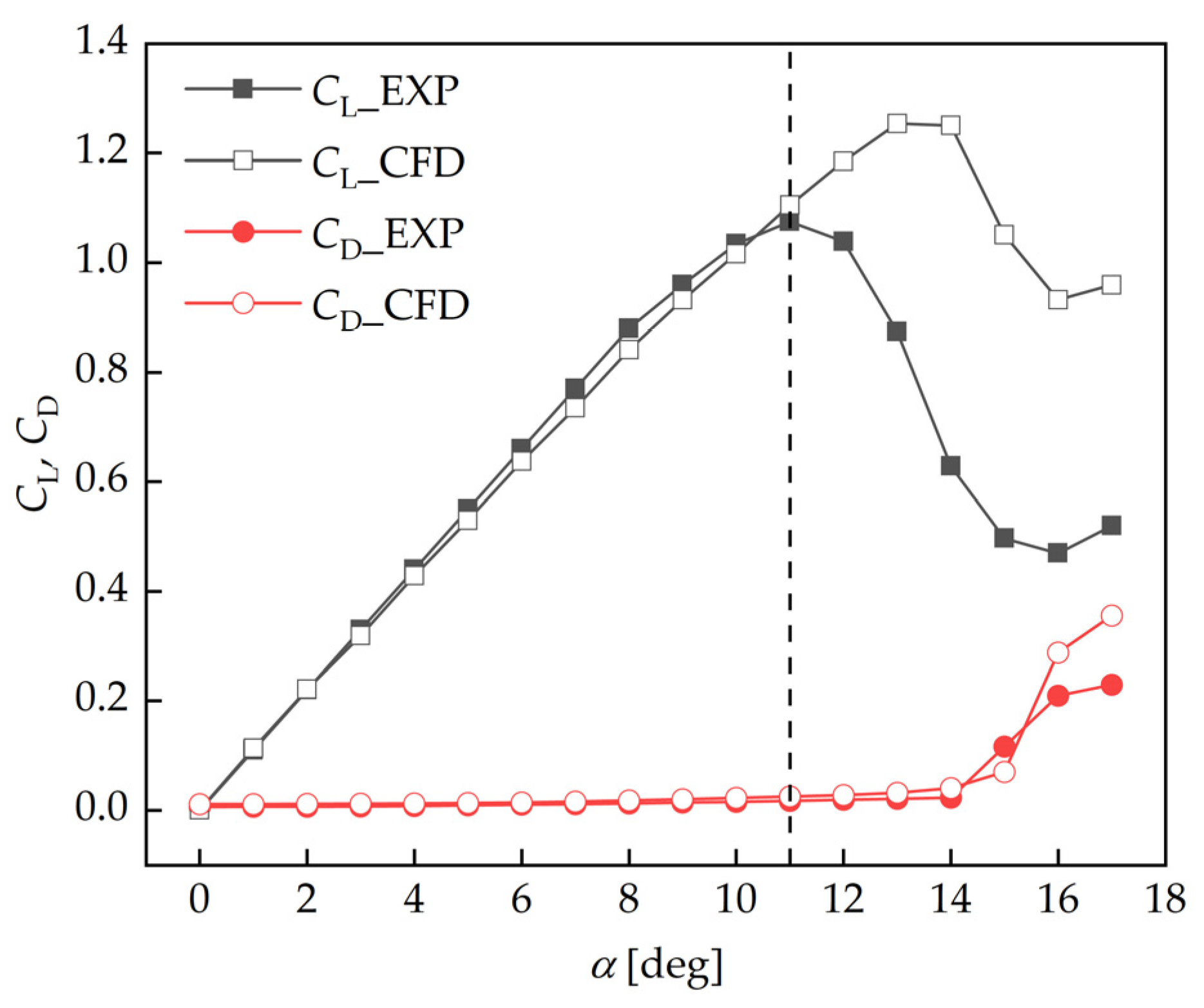
Selecting a validated model for preliminary CFD studies provides confidence in the numerical methods before applying them to the wingsail cases under investigation. Due to the fact that both the bare and concave three-element wingsails are designed based on the NACA0012 airfoil and the publicly available literature on three-element wingsail model experiments is limited, an NACA0012 airfoil from the wind tunnel test by Sheldahl [17] is selected as the numerical model. The simulation tests are conducted at AOA from 0 to 17 degrees, with a Reynolds number of 700,000. The numerical simulation results in this paper are compared with the experimental results, as shown in Figure 10. The results indicate that within an AOA range of 0 to 10 degrees, the values and trends of the lift coefficient and drag coefficient are in good agreement with the experimental results. However, beyond an AOA of 11 degrees, the numerical simulation results exhibit significant deviations, attributed to the unsteady flow behavior at higher AOAs, particularly beyond the stall. Therefore, the subsequent numerical simulations in this paper are conducted for AOAs ranging from 0 to 10 degrees.

Figure 10.
Comparison of lift and drag coefficients between CFD and experiment.
3. Numerical Results
After verifying the feasibility of the numerical approach, applying the validated CFD methodology to the wingsails can reveal quantified aerodynamic differences between the bare and concave design. Firstly, the aerodynamic and auxiliary propulsion performance of unfolded wingsails is studied, and its mechanism is analyzed from the corresponding flow field. Then, considering the foldable properties of the wingsails, the thrust performance is evaluated for a single rotation of the nose and flap separately. Finally, both the nose and flap are rotated to find the target folding configuration that produces the maximum thrust coefficient.
3.1. Wingsails without Camber
3.1.1. Lift and Drag Coefficient
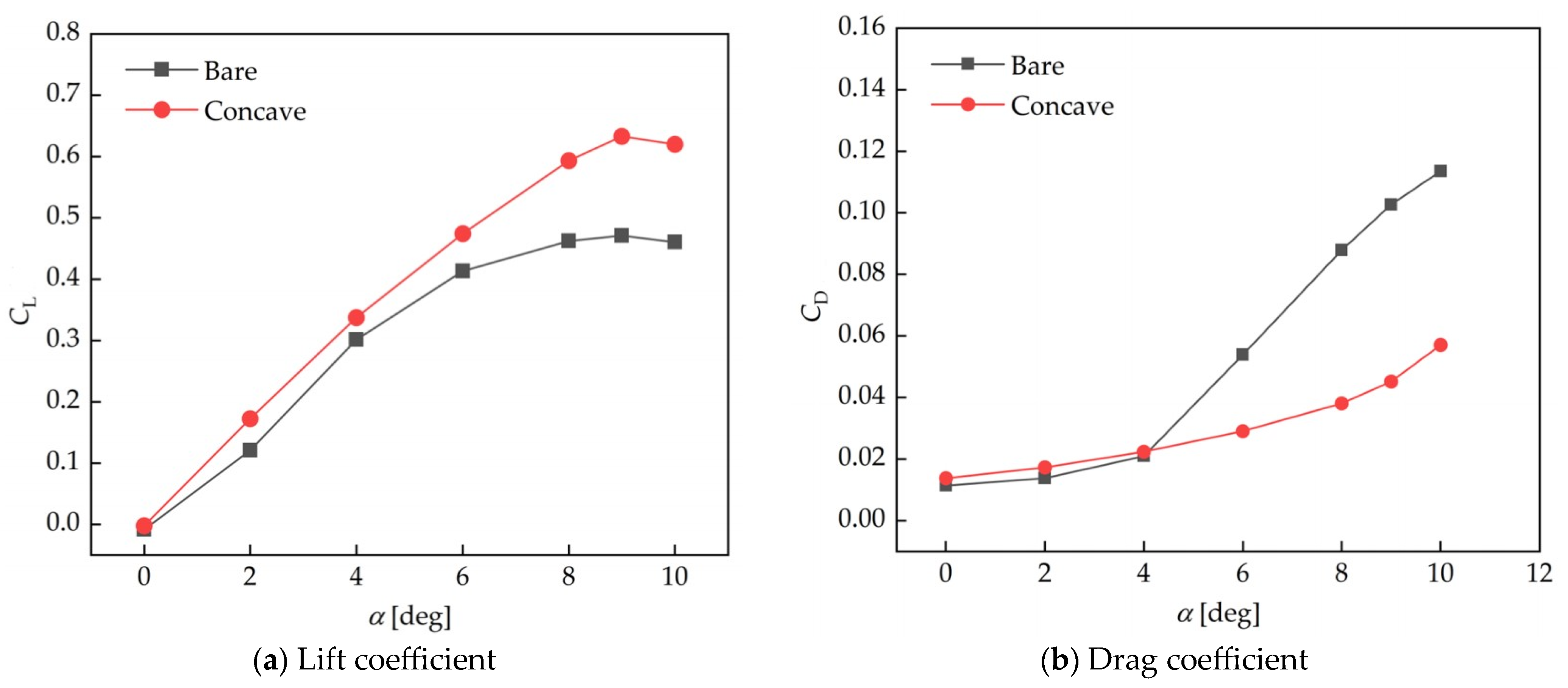
Since the aerodynamic performance of the wingsails is sensitive to AOA, the performance of an unfolded bare and concave wingsail at different AOAs is evaluated first. The lift and drag coefficients of the bare and concave wingsails are investigated in the AOA range of 0 to 10 degrees (as shown in Figure 11). The results show that the lift coefficients of both bare and concave wingsails increase in the range of AOA from 0 to 9 degrees, but a decreasing trend occurs at 10 degrees, with maximum lift coefficient values of 0.47 and 0.63 for bare and concave wingsails, respectively. In addition, the drag coefficients all increase with an increasing AOA. However, the analysis reveals that the difference in lift coefficients between the bare and concave wingsail increases significantly at an AOA greater than 4 degrees, and the drag coefficients similarly differ significantly at an AOA greater than 4 degrees, which may be related to the large change in the flow field, as will be further elaborated on later.
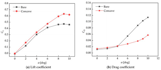
Figure 11.
Force coefficients of the wingsails.
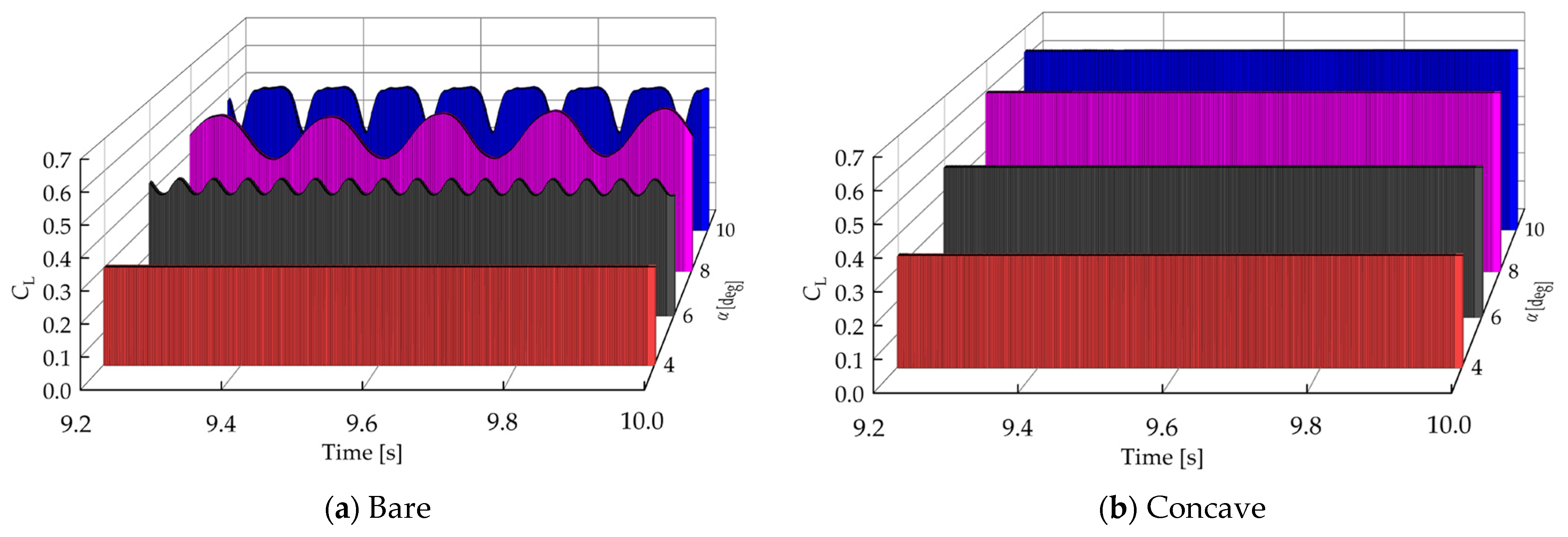
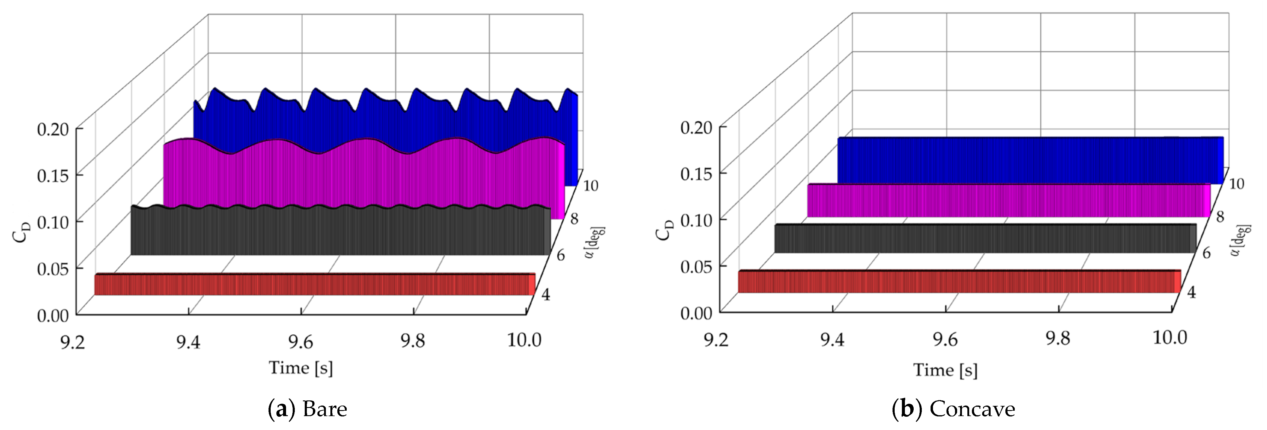
The time history curves of the lift and drag coefficients can help explain the abrupt changes in aerodynamics (as shown in Figure 12 and Figure 13). The results show that the time-course curve of both the lift and drag coefficients of a bare wingsail are straight lines when the AOA is 4 degrees, i.e., the lift and drag coefficients show no fluctuations. However, when the angle of attack is 6, 8, and 10 degrees, the curves of both the lift and drag coefficients show significant fluctuations, which are also due to changes in the flow field pattern around the wingsail. In contrast, the time history curves of the lift and drag coefficients of the concave wingsail do not show any fluctuation at all AOAs, indicating that the flow field pattern around the wingsail is more stable. The aerodynamic performance differences between the bare and concave wingsail will be mechanically explained in the following sections with detailed characteristics of the flow field.
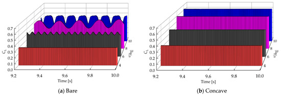
Figure 12.
Time history curves of lift coefficients of the wingsails.

Figure 13.
Time history curves of drag coefficients of the wingsails.
3.1.2. Thrust Coefficient
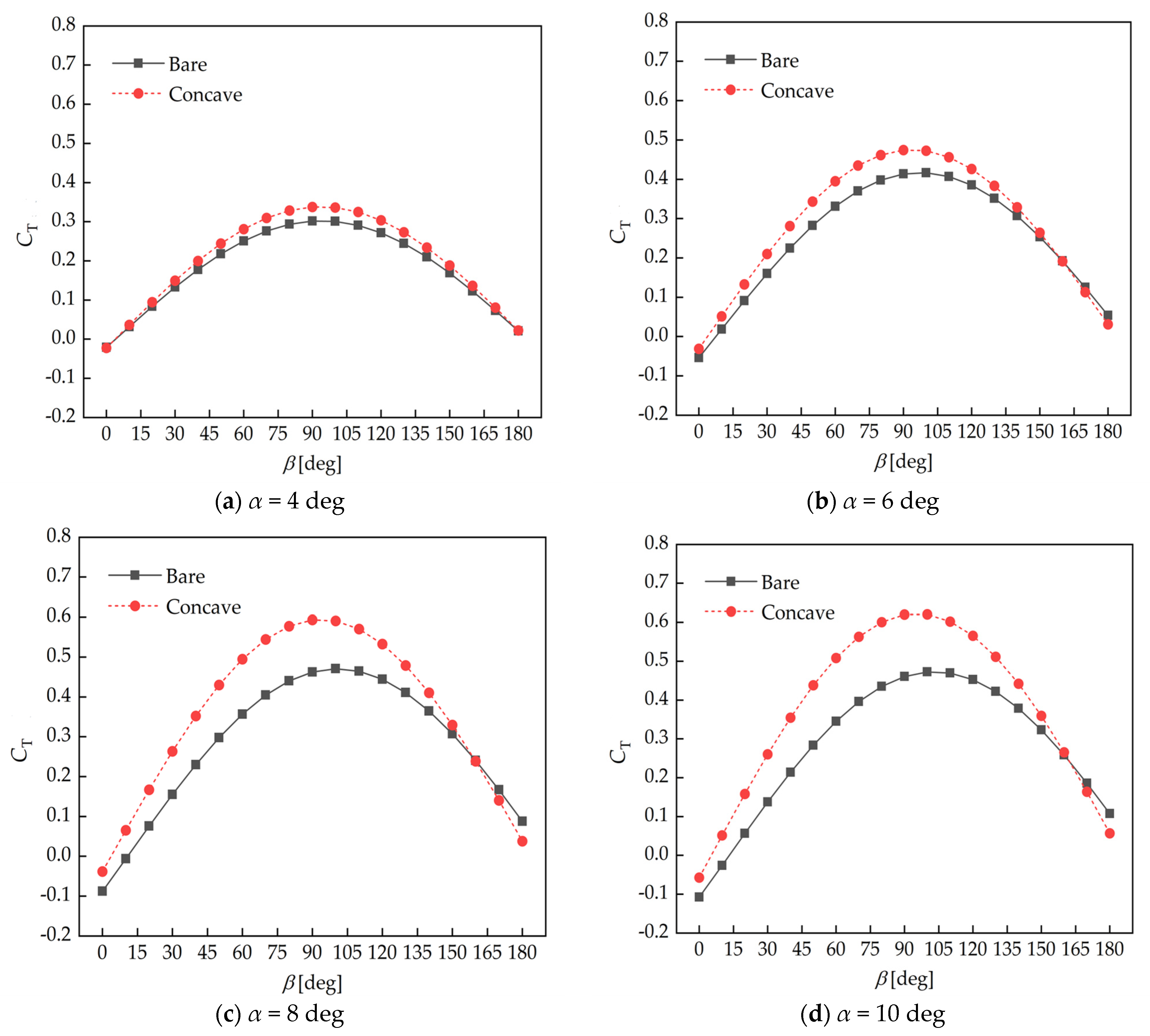
Focusing on thrust coefficients provides a more directly applicable perspective compared with individual lift and drag values when evaluating wingsail performance for maritime propulsion. As shown in Figure 14, a consistent increasing and then decreasing trend of the thrust coefficients for both bare and concave wingsails occurs at AOAs of 4, 6, 8, and 10 degrees, with peak values occurring around an AWA of 90 degrees. This indicates that wingsails are the most effective in practice when the apparent wind is a crosswind, and the crosswind direction is perpendicular to the vessel heading. In addition, the analysis reveals that the thrust coefficients of the concave wingsail are greater than those of the bare wingsail over most of the AWA range, and this difference increases with an increasing AOA. At an AOA of 10 degrees, the maximum thrust coefficients of the bare and concave wingsails are 0.47 and 0.62, respectively, with a difference of 32%.
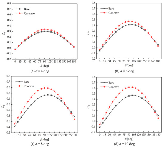
Figure 14.
Thrust coefficients of the wingsails at different AOAs and AWAs.
3.1.3. Flow Pattern
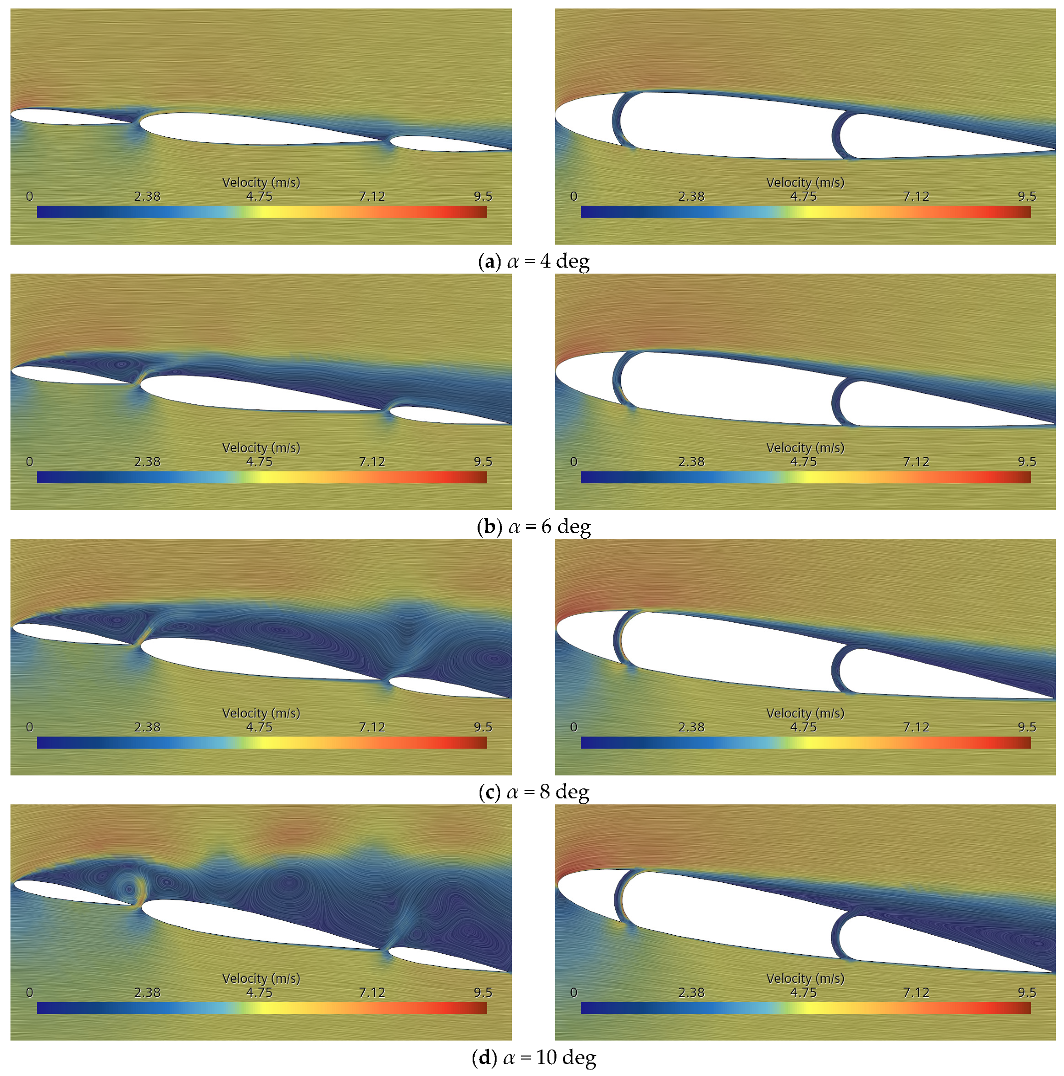
Analyses of the detailed characteristics of the flow field around the wingsails, such as velocity contours and vortex shedding patterns, can provide mechanistic explanations of the previous findings. The flow field patterns around the bare and concave wingsails at AOAs of 4, 6, 8, and 10 degrees are shown in Figure 15. The results indicate that the flow field on the surface of the bare wingsail remains stable at an AOA of 4 degrees. However, when the AOA is increased to 6 degrees, vortex shedding initiates on the suction side of the nose. As the AOA is further increased to 8 and 10 degrees, this vortex shedding pattern becomes more complex and intense, which explains the large fluctuation observed in the force coefficient curves. In contrast, the flow field on the suction side of the concave wingsail remains relatively stable across all AOAs. In addition, at an AOA of 10 degrees, slight flow separation occurs on the suction side of the concave wingsail’s flap, resulting in the high-velocity fluid moving away, thereby reducing the pressure difference. This corresponds to the sudden decrease in the lift coefficient (as shown in Figure 8).
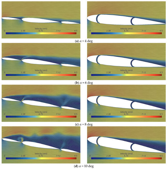
Figure 15.
Flow pattern around the wingsails at different AOAs.
The velocity contours for the two wingsails are also notably different, as shown in Figure 16. The results indicate that, while the velocity distributions are similar on the pressure side, they significantly differ on the suction side. For the bare wingsail, flow separation occurs at the leading edge of the nose, causing the high-velocity fluid to move away from the surface of the wingsail, resulting in a lower pressure difference and thus a lower lift coefficient. In contrast, for the concave wingsail, flow separation on its suction side occurs at the trailing edge of the nose, leading to the better adsorption of high-speed fluids and a narrower low-speed zone. This difference results in a higher pressure difference between the two sides of the wingsail, thereby leading to a higher lift coefficient, which confirms previous aerodynamic findings.
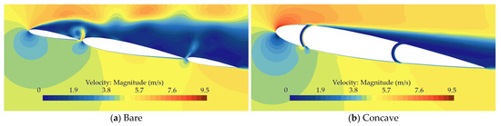
Figure 16.
Velocity contours of the wingsails (α = 10 deg).
Furthermore, from the flow field of the bare wingsail, it can be seen that the pattern of incoming airflow changes significantly when it is approaching the gaps. In conjunction with the analysis above, it can be seen that it is the larger and wider flow separation zone, which result in some airflow on the pressure side passing through the gaps under negative pressure. In addition to this, this part of airflow will be accelerated by the gaps to rush into the suction side at a higher velocity, which will interfere with the flow separation.
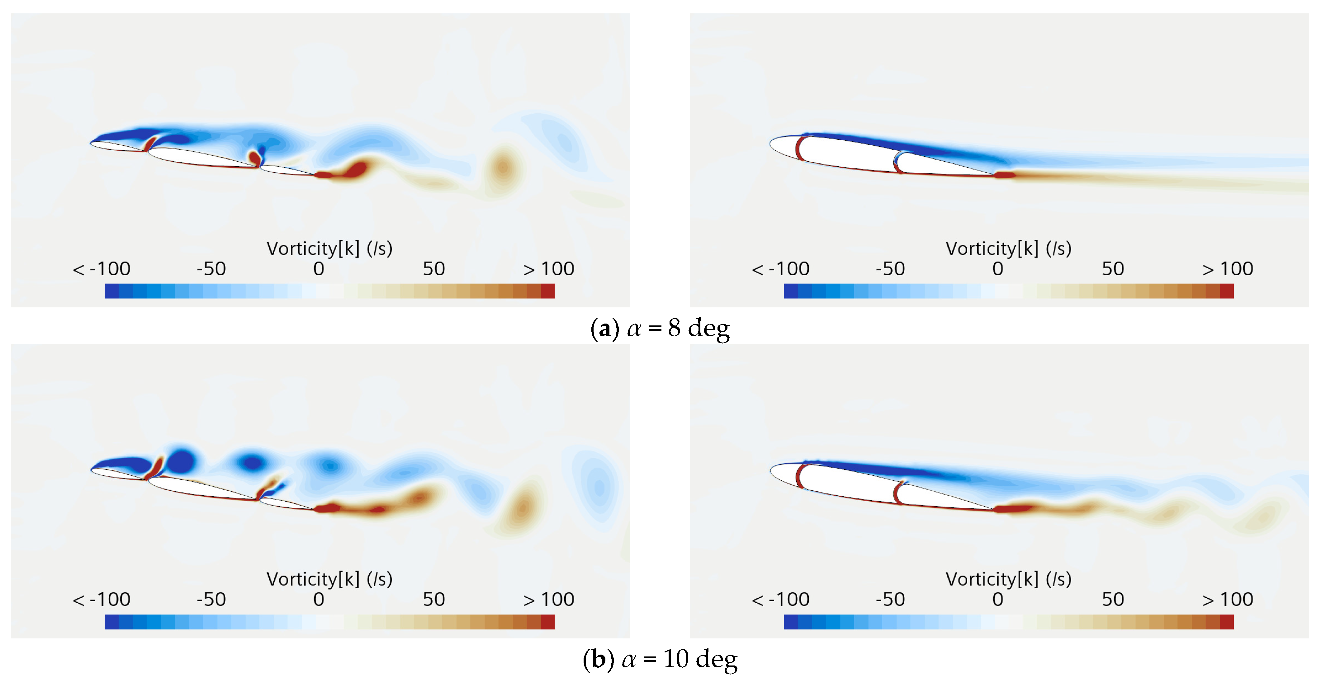
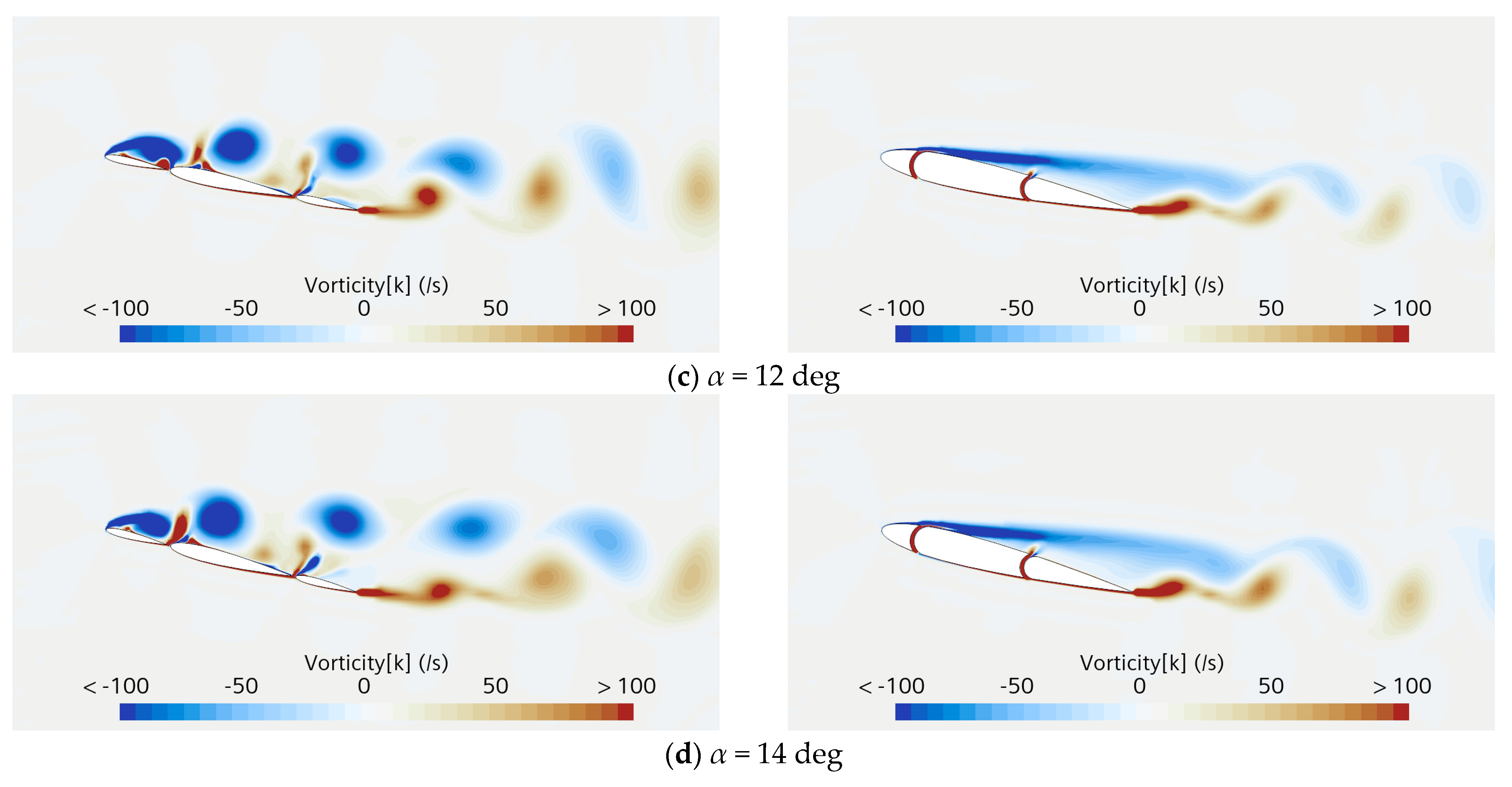
In order to obtain a comprehensive understanding of the aerodynamic performance of both the bare and concave wingsails, we have continued to study the aerodynamic performance at higher AOAs. As shown in Figure 17, it is found that when the AOA is greater than 10 degrees, the vortex shedding patterns on the suction side of the original wingsail (bare wingsail) are similar, while the vorticity intensity increased along with it. Similarly, the steady flow on the suction side of the optimized wingsail (concave wingsail) gradually evolves into a periodic vortex shedding pattern, and the vorticity intensity is also significantly increased. In engineering applications, the high-intensity vortex shedding will cause unstable aerodynamic performance, and the oscillating lift and drag can cause fatigue of the wingsails’ structures. In the present study, we focus on the stable and efficient aerodynamic performance of wingsails. Therefore, further research will mainly focus on medium and small attack angles in the following text.
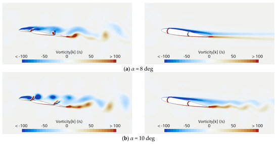
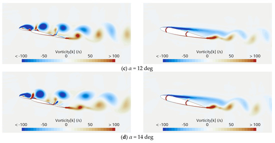
Figure 17.
Vorticity distribution around the wingsails at different AOAs.
3.2. Wingsails with Camber
3.2.1. Definition of Camber
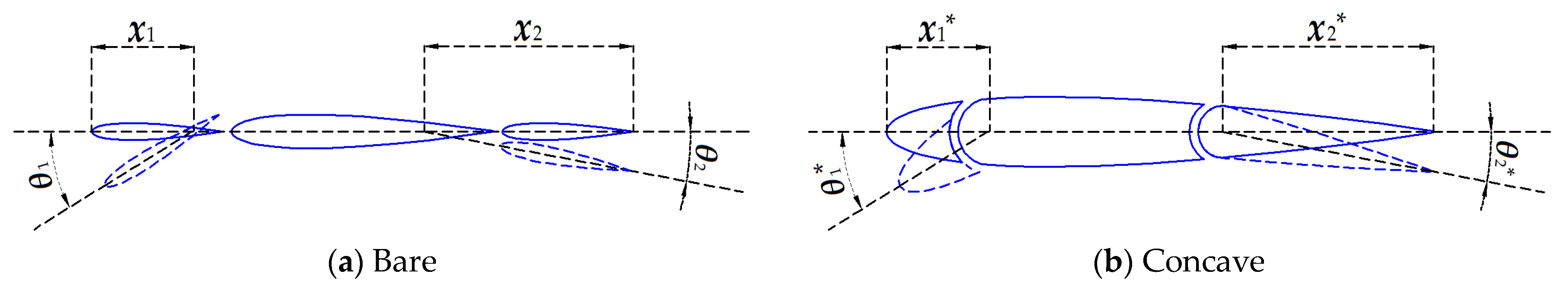
In order to assess the differences between bare and concave wingsails with different folding patterns, a camber is introduced, as depicted in Figure 18. θ1 and θ1* represent the camber angle of the nose, while θ2 and θ2* represent the camber angle of the flap. To simplify this study, the position of the pivot is kept the same for both wingsails, with x1 = x1* = 0.2 c, and x2 = x2* = 0.4 c. In practical engineering applications, the nose (or flap) and main body are connected by hydraulic telescopic rods, and the two ends of the rods are fixed on the rotating axes of the nose (or flap) and main body, respectively. This mechanism of attachment ensures that the nose and flap can generate cambers to further enhance the thrust performance. The effects of these two components are first evaluated separately in this paper and then collectively in a subsequent study.
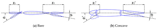
Figure 18.
Parameterization of the camber and the pivot location of the wingsails.
3.2.2. Individual Evaluation for Nose and Flap Cambers
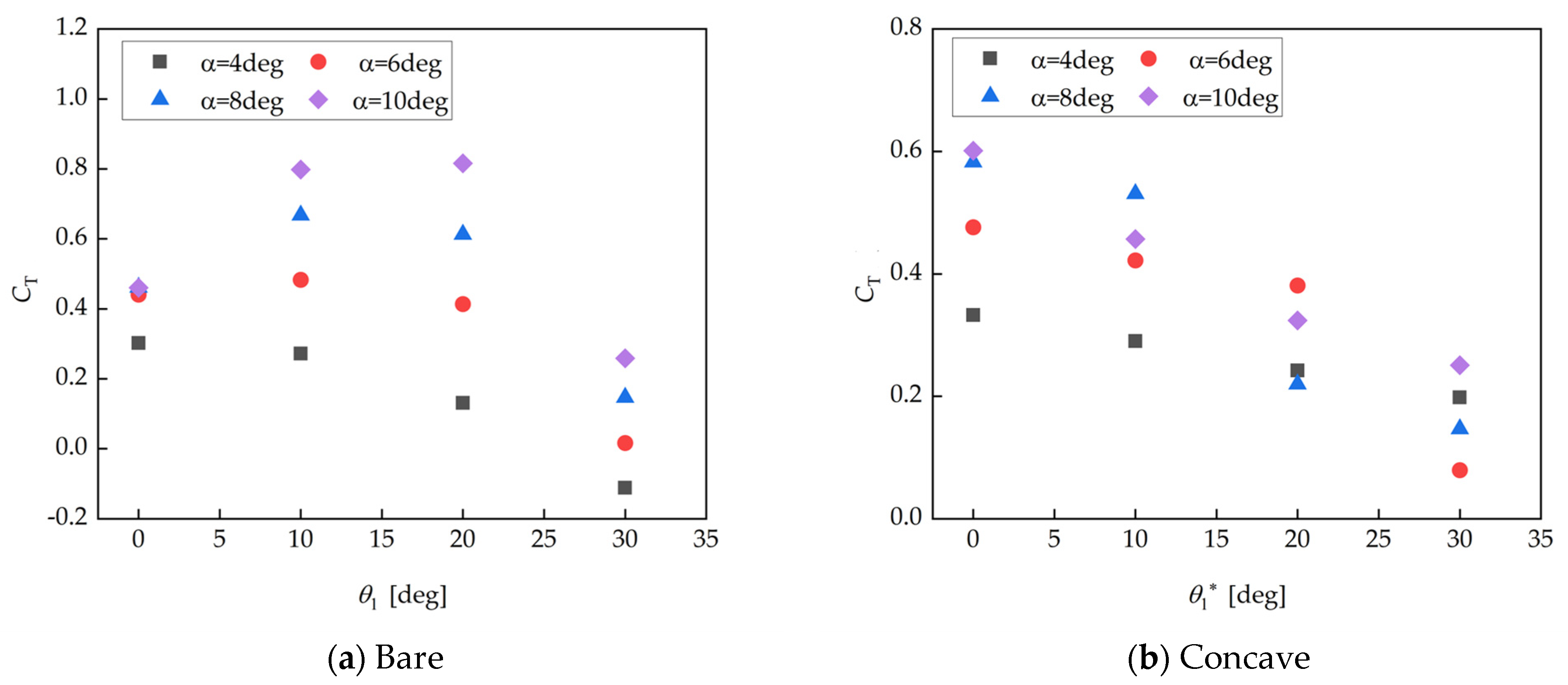
The thrust coefficients of the two wingsails are evaluated at AOAs of 4, 6, 8, and 10 degrees when rotating the nose and flap separately. Figure 19 shows the thrust coefficient results of bare wingsails and concave wingsails when only the nose rotates. Within the camber range of 0 to 30 degrees, the thrust coefficient of the bare wingsail exhibits a trend of initially increasing and then decreasing. Both the optimal camber angle of the nose and the corresponding thrust coefficient increase with the AOA. Conversely, the thrust coefficient of the concave wingsail shows a monotonically decreasing trend, which indicates that increasing the camber angle of the nose can enhance the thrust performance of the bare wingsail but is detrimental to the concave wingsail. In addition, the trend of the thrust coefficient is generally similar across different AOAs, and an AOA of 8 degrees is selected for a quantitative comparative analysis. The maximum thrust coefficient values for the bare and concave wingsails are achieved at nose camber angles of 10 and 0 degrees, respectively, measuring 0.67 and 0.58, with a difference of 15.5%.
Figure 19.
Thrust coefficient of the wingsails at different cambers of the nose.
Figure 20 shows the thrust coefficient results of bare and concave wingsails with only the flap rotating. Within the camber range of 0 to 70 degrees, the thrust coefficients of both the bare and concave wingsails exhibit a trend of initially increasing and then decreasing. This suggests that rotating the flap enhances the thrust performance of both the bare and concave wingsails, and this effect is more significant than that of the nose. Similarly, quantitative comparisons are conducted at an AOA of 8 degrees. The analysis shows that the bare and concave wingsails achieve maximum values of 1.47 and 2.06 at a flap camber angle of 50 degrees, respectively, representing a difference of 40.1%. In addition, the thrust coefficient is improved by 19.0% and 53.5%, respectively, compared with the unfolded configuration.
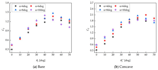
Figure 20.
Thrust coefficient of the wingsails at different cambers of the flap.
3.2.3. Parallel Evaluation for Nose and Flap Cambers
In order to explore the folding configuration of the bare and concave wingsails when the thrust coefficients are optimal, parallel simulations are conducted for the combination with the nose and flap at different cambers (as shown in Figure 21). Based on the results of a single evaluation of the nose and flap in the previous section, a range of 0 degrees to 20 degrees is determined to vary the interval of the nose camber and 40 degrees to 50 degrees to vary the interval of the flap camber, resulting in 25 scenarios for each wingsail. In addition, since the variation trends of the thrust coefficient with a nose camber or flap camber are almost similar at different AOAs, a parallel study is carried out at an AOA of 8 degrees to simplify the analysis. The results indicate that the bare wingsail achieves a maximum thrust coefficient of 1.7 at a nose camber of 20 degrees and a flap camber of 50 degrees, while the concave wingsail reaches a maximum thrust coefficient of 2.1 at a nose camber of 15 degrees and a flap camber of 50 degrees, thus achieving an optimization of 23.5%. Furthermore, the comparison reveals that the thrust coefficients of the concave wingsail are higher than those of the bare wingsail in most of the folding configurations.
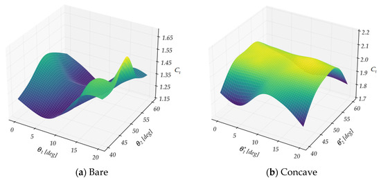
Figure 21.
Thrust coefficient of the wingsails at different cambers of both the nose and flap.
Through the above research, the optimal folding configuration of the wingsail is obtained. The camber angle of the bare wingsail’s nose and flap is 20 degrees and 50 degrees, respectively, while for the concave wingsail, it is 15 degrees and 50 degrees, respectively. In order to provide a mechanical explanation of the performance difference, the pressure distribution around the wingsail is analyzed (as shown in Figure 22). The results show significant differences in pressure distributions on both the pressure and suction sides. On the pressure side of the bare wingsail, the airflow passes directly through the gap between the main body and flap, resulting in a reduction in the extent of the high-pressure area. Furthermore, the low-pressure area on the suction side of the concave wingsail is much more extensive and continuous, with distinct low-pressure areas occurring on both the suction side of the nose and main body. Consequently, the pressure difference between the two sides is greater, resulting in higher lift, particularly at an AWA of approximately 90 degrees, where the concave wingsail optimally utilizes wind energy, converting lift almost entirely into thrust. In particular, the suction side of the bare wingsail’s flap also appears to have a significant low-pressure area. However, because this low-pressure area is located behind the flaps, it has little effect on lift, mainly leading to an increase in drag.
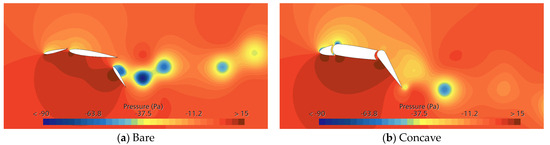
Figure 22.
Pressure distribution around the wingsails (AOA = 8 deg).
After obtaining the maximum thrust coefficient, the performance of the wingsail in utilizing wind energy to reduce the energy consumption of vessels can be further evaluated. As shown in Equations (5) and (6), is the speed of the vessel, is the thrust of the wingsail, is the power of the wingsail, is the surface area of the wingsail, and is the maximum thrust coefficient. The specific values of the above parameters are shown in Table 3. For a wingsail with a chord length of 1 m and a unit span length, its surface area S is 1 m2. Thus, the per unit wingsail surface area can provide an auxiliary propulsion power of 32.2 W per unit vessel speed. The calculations here consider the wingsails as an individual model and neglect the effects of waves in real sea states. In fact, the wingsails and deck are rigidly connected, which means the motion of the vessels will be affected by the coupling effect of wind and wave loads. This will disrupt the incoming airflow pattern, causing the wingsails to be unable to generate stable thrust and resulting in a certain loss of thrust power. In future studies, the coupling effect on the three-dimensional scale will be studied to reflect the auxiliary propulsion performance in a more comprehensive way.
Table 3.
Partial flow field parameters.
4. Conclusions
The performances of two types of three-element foldable wingsails, i.e., the original model (bare wingsail) and an optimized model (concave wingsail), are numerically investigated using the CFD method. By integrating quantitative performance metrics with an analysis of the physics governing wingsail aerodynamics, this work enables data-driven guidelines for balancing thrust capability, flow stability, and practicable engineering considerations in the design and application of wingsails, and the main conclusions are presented below.
- In an unfolded state, the aerodynamic and thrust performance of the concave wingsail is superior to that of the bare wingsail. In an AOA range of 4 to 10 degrees, the concave wingsail has a higher lift coefficient and lower drag coefficient, which results in a higher thrust performance for the same AOA and AWA. In addition, the flow pattern on the surface of the concave wingsail is consistently stable, with no significant vortex shedding, which indicates that the thrust performance is more stable.
- When evaluating the effect of the nose and flap cambers individually, it is found that rotating only the flap can significantly increase the thrust coefficients of both the bare and concave wingsails. However, it should be noted that the thrust coefficients decrease when the nose and flap cambers increase to certain critical values. In summary, the suitable variation interval for the nose and flap cambers are 0 to 20 degrees and 40 to 60 degrees, respectively.
- The thrust performance of both wingsails is further improved in the fully folded condition, i.e., when both the nose and flap are rotated. The maximum thrust coefficient of the bare wingsail is 1.7, when the nose’s camber is equal to 20 degrees and the flap’s camber is equal to 50 degrees. As for the concave wing, the maximum thrust coefficient is 2.1, at which the nose’s camber is equal to 15 degrees and the flap’s camber is equal to 50 degrees. In particular, at an AOA of 8 degrees, the thrust coefficient of the concave wingsail is increased by 23.5% compared with the bare wingsail.
Author Contributions
Conceptualization, Y.J.; methodology, C.C.; software, C.C.; validation, T.C.; formal analysis, T.C.; investigation, C.C.; resources, Z.T.; data curation, Z.T.; writing—original draft preparation, C.C.; writing—review and editing, H.Y.; visualization, C.C. and H.Y.; supervision, Y.J. All authors have read and agreed to the published version of the manuscript.
Funding
This research received no external funding.
Data Availability Statement
Data is contained within the article.
Conflicts of Interest
The authors declare no conflict of interest.
Nomenclature
| c | total chord of the wingsail [m] |
| c1, c1* | chord of the nose of the wingsail [m] |
| c2, c2* | chord of the main body of the wingsail [m] |
| c3, c3* | chord of the flap of the wingsail [m] |
| g1, g1, g1*, g2* | gap of the wingsail [m] |
| Re | Reynolds number [-] |
| U | velocity of the inlet flow [m/s] |
| Δt | time step [s] |
| CL | lift coefficient [-] |
| CD | drag coefficient [-] |
| CT | thrust coefficient [-] |
| VA | apparent wind speed [m/s] |
| VS | sailing wind speed [m/s] |
| VT | true wind speed [m/s] |
| FL | lift force [N] |
| FD | drag force [N] |
| FT | thrust force [N] |
| α | angle of attack [deg] |
| β | angle of apparent wind [deg] |
| θ1, θ1* | camber angle of nose of the wingsail [deg] |
| θ2, θ2* | camber angle of flap of the wingsail [deg] |
| x1, x1* | pivot location of nose of the wingsail [-] |
| x2, x2* | pivot location of nose of the wingsail [-] |
References
- Joung, T.H.; Kang, S.G.; Lee, J.K.; Ahn, J. The IMO initial strategy for reducing Greenhouse Gas (GHG) emissions, and its follow-up actions towards 2050. J. Int. Marit. Saf. Environ. Aff. Ship. 2020, 4, 1–7. [Google Scholar] [CrossRef]
- Available online: https://www.dnv.com/news/imo-mepc-80-shipping-to-reach-net-zero-ghg-emissions-by-2050-245376 (accessed on 7 July 2023).
- Nyanya, M.N.; Vu, H.B. Wind Propulsion Optimisation and Its Integration with Solar Power. Ph.D. Thesis, World Maritime University, Malmö, Sweden, 2019. [Google Scholar]
- Julià Lluis, E. Concept Development of a Fossil Free Operated Cargo Ship. Ph.D Thesis, Chalmers University of Technology, Gothenburg, Sweden, 2019. [Google Scholar]
- Available online: https://www.offshore-energy.biz/dnv-greenlights-oceanbirds-wing-sail/ (accessed on 29 August 2023).
- Available online: https://www.prnewswire.com/news-releases/berge-bulk-unveils-the-worlds-most-powerful-sailing-cargo-ship-301955875.html (accessed on 16 October 2023).
- Furukawa, H.; Blakeley, A.W.; Flay, R.G.; Richards, P.J. Performance of wing sail with multi element by two-dimensional wind tunnel investigations. J. Fluid Sci. Technol. 2015, 10, JFST0019. [Google Scholar] [CrossRef]
- Schneider, A.; Arnone, A.; Savelli, M.; Ballico, A.; Scutellaro, P. On the use of CFD to assist with sail design. In Proceedings of the SNAME Chesapeake Sailing Yacht Symposium, Annapolis, MD, USA, 3 March 2003. [Google Scholar]
- Li, C.; Wang, H.; Sun, P. Numerical investigation of a two-element wingsail for ship auxiliary propulsion. J. Mar. Sci. Eng. 2020, 8, 333. [Google Scholar] [CrossRef]
- Li, C.; Wang, H.; Sun, P. Study on the Influence of Gradient Wind on the Aerodynamic Characteristics of a Two-Element Wingsail for Ship-Assisted Propulsion. J. Mar. Sci. Eng. 2023, 11, 134. [Google Scholar] [CrossRef]
- Blakeley, A.W.; Flay, R.G.J.; Richards, P.J. Design and optimisation of multi-element wing sails for multihull yachts. In Proceedings of the 18th Australasian Fluid Mechanics Conference, Launceston, Australia, 3–7 December 2012. [Google Scholar]
- Ma, R.; Wang, Z.; Wang, K.; Zhao, H.; Jiang, B.; Liu, Y.; Xing, H.; Huang, L. Evaluation Method for Energy Saving of Sail-Assisted Ship Based on Wind Resource Analysis of Typical Route. J. Mar. Sci. Eng. 2023, 11, 789. [Google Scholar] [CrossRef]
- Shen, X.; Avital, E.; Rezaienia, M.A.; Paul, G.; Korakianitis, T. Computational methods for investigation of surface curvature effects on airfoil boundary layer behavior. J. Algorithms Comput. Technol. 2017, 11, 68–82. [Google Scholar] [CrossRef]
- Bilandi, R.N.; Jamei, S.; Roshan, F.; Azizi, M. Numerical simulation of vertical water impact of asymmetric wedges by using a finite volume method combined with a volume-of-fluid technique. Ocean. Eng. 2018, 160, 119–131. [Google Scholar] [CrossRef]
- Hassan, G.E.; Hassan, A.; Youssef, M.E. Numerical investigation of medium range re number aerodynamics characteristics for NACA0018 airfoil. CFD Lett. 2014, 6, 175–187. [Google Scholar]
- Blount, H.; Portell Lasfuentes, J.M. CFD Investigation of Wind Powered Ships under Extreme Conditions. Master’s Thesis, Chalmers University of Technology, Gothenburg, Sweden, 2021. [Google Scholar]
- Sheldahl, R.E.; Klimas, P.C. Aerodynamic Characteristics of Seven Symmetrical Airfoil Sections through 180-Degrees Angle of Attack for Use in Aerodynamic Analysis of Vertical Axis Wind Turbines (No. SAND-80-2114); Sandia National Lab (SNL-NM): Albuquerque, NM, USA, 1981. [Google Scholar]


Disclaimer/Publisher’s Note: The statements, opinions and data contained in all publications are solely those of the individual author(s) and contributor(s) and not of MDPI and/or the editor(s). MDPI and/or the editor(s) disclaim responsibility for any injury to people or property resulting from any ideas, methods, instructions or products referred to in the content. |
© 2024 by the authors. Licensee MDPI, Basel, Switzerland. This article is an open access article distributed under the terms and conditions of the Creative Commons Attribution (CC BY) license (https://creativecommons.org/licenses/by/4.0/).