Numerical Calculation and Application for Crushing Rate and Fracture Conductivity of Combined Proppants

Abstract

Proppant is one of the key materials for hydraulic fracturing. For special situations, such as middle-deep reservoirs and closure pressures ranging from 40 MPa to 60 MPa, using a single proppant cannot solve the contradiction between performance, which means crushing rate and fracture conductivity, and cost. However, using combined proppants is an economically effective method for hydraulic fracturing of such special reservoirs. Firstly, for different types, particle sizes, and proportions of combined proppants, various contact relationships between proppant particles are considered. The random phenomenon of proppant particle arrangement is described using the Monte Carlo method, and the deterministic phenomenon of proppant particles is processed using an optimization model, achieving computer simulation of the microscopic arrangement of proppant particles. Secondly, a mathematical model for the force analysis of combined proppant particles is established, and an improved singular value decomposition method is used for numerical solution. A computational model for the crushing rate and fracture conductivity of combined proppants is proposed. Thirdly, the numerical calculation results are compared and discussed with the test values, verifying the accuracy of the computational model. Finally, the application of combined proppants is discussed, and a model for optimizing the proportion of combined proppants is proposed. The onsite construction technology is introduced, and the cost and economic benefits of combined proppants are compared with those of all ceramic particles and excessive all-quartz sand. It is proved that combined proppants can balance performance and price, and are an economically effective method for hydraulic fracturing of special reservoirs. The research results can select the optimal proppant material and optimize the combination of different proppant types, which can help achieve cost reduction and efficiency increase in oil and gas development.

1. Introduction

Hydraulic fracturing, as an important measure and main method for increasing storage and production as well as effective development of oil and gas fields [1,2], has already and will increasingly play an important role in energy demand and economic development. Proppant is one of the key main materials of hydraulic fracturing. Its main function is to support fractures and create channels with high conductivity for fluid flow in fractures. In order to meet the needs of hydraulic fracturing in different reservoirs and deep wells, at present, various types of proppants have been developed, mainly including quartz sand, ceramsite, coated sand, and low-density proppants. Important factors must be considered. The contradiction between the performance and price of proppants (Figure 1) is one of the bottlenecks in the economic and effective development of oil and gas reservoirs [3,4,5].

Scholars have studied the optimization of injection strategies for proppant based on the response of key parameters to injection [6,7,8,9]. In addition, there have been studies on the transportation [10,11,12,13] and distribution [14,15] of proppant in hydraulic fracture. In these studies, simulation experiments of proppant injection were conducted, and simulation models of proppant transportation were established, laying the research foundation for the performance parameters of proppant.

The crushing rate and fracture conductivity of proppant are key parameters for evaluating the performance [16,17]. The crushing rate is the performance indicator that characterizes the compressive strength of a proppant, which refers to the fragmentation of a group of proppant particles under a specified closing pressure. The higher the crushing rate of the proppant, the smaller the space for fluid flow in the fracture, and the lower the fracture conductivity. Therefore, the crushing rate of proppants directly affects the success or failure of hydraulic fracturing or the production of wells. The crushing rate of proppants is an important parameter indicator for studying the fracture conductivity. The fragmentation and embedding of proppants are the main factors affecting the fracture conductivity, while the particle size, shape, concentration, and acid solubility of proppants are secondary factors affecting the fracture conductivity.

Currently, there are three methods for studying the performance parameters of proppants. The first method is to test the performance indicators of the proppant through physical experiments [18,19,20]. However, due to the different or even significant differences in the performance of proppants, physical experimental methods, especially those for fracture conductivity, mainly exhibit long testing time, small coverage, and high testing costs. At the same time, test results under the same conditions are unstable and even have large errors [21,22,23,24,25]. The second method is based on physical experiments and is combined with numerical simulation to study the performance parameters of proppants [26,27,28]. However, most models are empirical or semiempirical mathematical models established on the premise of ignoring the crushing rate of proppants or assuming ideal conditions [29,30,31,32,33]. The third method is supported by simple and economical crushing rate experiments, using microscopic modeling and numerical calculations to obtain the fracture conductivity of the proppant, and solving the limitations of physical experiments [34]. In 2021, Guo et al. [35] considered the characteristic that proppants have different particle sizes in their arrangement but are distributed within a specific numerical interval. Using the same type of proppant with different particle sizes, they evaluated the proppant crushing rate and fracture conductivity.

For special situations, such as middle-deep reservoirs and closure pressures ranging from 40 MPa to 60 MPa, using a single type of proppant cannot solve the contradiction between performance, which means crushing rate and fracture conductivity, and cost. In other words, it is necessary to study a low-cost and effective proppants scheme. As mentioned above, the method of physical experiments has obvious limitations. The existing numerical simulation methods are based on the assumption of ideal conditions and ignore the combination of different types, particle sizes, and ratios of proppants. However, using combined proppants is an economically effective method for hydraulic fracturing of such special reservoirs. Therefore, starting from the microscopic arrangement mechanism of proppants, an attempt is made to establish a mathematical model for combined proppants and to conduct computer simulations on crushing rate and fracture conductivity. The goal of the research is to overcome the shortcomings of existing studies and propose a new computer simulation method for the crushing rate and fracture conductivity of combined proppants, and, furthermore, to select the optimal type and combination of proppants to achieve cost reduction and increased efficiency in hydraulic fracturing. The advantages of the combined proppant are analyzed in the construction test, and the problems and innovations solved are as follows:

(1) According to the proportion of different types of proppant in the combined proppant, we establish a mathematical model of different particle sizes of the combined proppant. (2) By studying the microarrangement mechanism of the combined proppant, based on the randomness and determinism in the particle arrangement of the combined proppant, a corresponding solution is proposed to realize the computer simulation of the combined proppant particles. (3) According to the properties of the combined proppant particles that may have different properties, different particle sizes, and different proportions, the calculation model of the crushing rate of the combined proppant is established. (4) According to the Kozeny–Garman equation, the permeability model of the combined proppant is established, and the mathematical model of the fracture conductivity of the combined proppant particles is established in combination with the actual situation of the fracture width reduction after the combined proppant particles are broken. (5) According to the actual situation of the closed pressure of the reservoir, through the optimization of the mixing ratio of the combined proppant, the research of the combined proppant construction technology, the design of the combined proppant fracturing operation, etc., cracked construction. Comparing with other production wells with sanding methods, we research and analyze the advantages of the combined proppant.

The organization of the remaining parts of this article is as follows. In the second part, a computer simulation model for the arrangement of combined proppant particles is established. The third part proposes a calculation method for the crushing rate of proppants and the fracture conductivity. The fourth part analyzes the calculation results of the particle arrangement, force simulation, crushing rate, and crack conductivity of the combined proppant. The fifth part is the construction effect of onsite application and analysis of typical wells. The sixth part is the conclusion and recommendations.

2. Computer Simulation of Micro Arrangement

For the study of combined proppant, firstly, the types and particle sizes of different proppants should be determined. Secondly, computer simulation of combined proppant particles should be conducted. Thirdly, mechanical modeling and calculation of combined proppant particles should be carried out. Finally, the stress on each particle of the combined proppant particles should be calculated to determine the crushing rate and fracture conductivity.

2.1. Particle Size Distribution

Combination proppants are different types and specifications of proppants (strength, density, particle size) mixed in different proportions, which can exert the support ability of high-strength proppants and the filling and diversion of low-strength proppants. Let ξ be a random number used to generate particle size. α₁ and α₂ are the respective proportions of two different types of proppants. The combined proppant particle size R obtained from these two types of proppants can be calculated from Equation (1).

$$R=\left\{\begin{array}{cc}{d}_1& \xi \in \left(0,{\displaystyle \frac{{\alpha }_1}{{\alpha }_1+{\alpha }_2}}\right)\\ d_2& \xi \in \left({\displaystyle \frac{{\alpha }_1}{{\alpha }_1+{\alpha }_2}},1\right)\end{array}\right.$$

(1)

Assuming there are k types of proppants, the combined proppant particle size R obtained from these k types of proppants can be calculated from Equation (2).

$$R=\left\{\begin{array}{cc}{d}_1& \xi \in \left(0,\frac{{\alpha }_1}{{\displaystyle \sum _{i=1}^k{\alpha }_i}}\right)\\ d_2& \xi \in \left(\frac{{\alpha }_1}{{\displaystyle \sum _{i=1}^k{\alpha }_i}},{\displaystyle \frac{{\displaystyle \sum _{i=1}^2{\alpha }_i}}{{\displaystyle \sum _{i=1}^k{\alpha }_i}}}\right)\\ ⋮& \hspace{1em}\hspace{1em}\hspace{1em}⋮\\ d_k& \xi \in \left({\displaystyle \frac{{\displaystyle \sum _{i=1}^{k-1}{\alpha }_i}}{{\displaystyle \sum _{i=1}^k{\alpha }_i}}},1\right)\end{array}\right.$$

(2)

where R represents the particle size of the combined proppant (mm). ξ is a random number used to generate particle size (dimensionless). d_i is the average particle size from any type of proppant (mm).

2.2. Physical Modeling and Computer Simulation

The arrangement of combined proppant particles in hydraulic fracturing fractures and the proppant performance testing device are consistent with the physical model with various particle sizes established by Guo [35]. It can also be modeled and solved in this way. When simulating the combined proppant particles, taking the combination of ceramic particles and quartz sand as an example, and setting the ratio of ceramic particles and quartz sand in advance, ceramic particles and quartz sand appear randomly based on random numbers. Under the boundary force P_c, the left and right boundaries change in the direction parallel to the force, but remain unchanged in the direction perpendicular to the force. The packing rules of particles are as follows [36,37,38,39,40,41,42]:

(1)

Set the ratio according to ceramsite and quartz sand, and randomly appear according to the proportion;

(2)

The first row is stacked from left to right;

(3)

The second row and above pile up one by one from bottom upwards;

(4)

The positioning of each particle is based on the minimum distance from its center to the bottom of the fracture;

(5)

When the position with the shortest distance between the particle circle center and the bottom boundary is unique, it is deterministic laying; otherwise, this position is not unique, and it is random laying.

Assume the width of the fracture in the x direction is w_f, and the length of the fracture in the y direction is L_f. Set the particle size of ceramsite to R^c and relate the granular size of quartz sand to R^s. In the coordinate system shown in Figure 2, the center coordinates of any proppant particle can be expressed as (x_i, y_i), and the aggregate count of particles in contact with the x-axis as the lower boundary can be calculated from Equation (3).

$$n_x=\mathrm{int}\left({\displaystyle \frac{w_f}{R^c+R^s}}\right)+\mathrm{int}\left({\displaystyle \frac{\mathrm{mod}(w_f,R^c+R^s)}{\min (R^c,R^s)}}\right)$$

(3)

where n_x is the count of circles touching the lower boundary (dimensionless). int(·) is rounding function. mod(·) is complementary function. min(·) is minimum function.

Under the given fracture length L_f and fracture width w_f, the arrangement of combined proppant particles can be divided into two forms: random and deterministic.

With a given width, the location of the distribution of proppant particles touching the lower boundary is random. Using the random number ξ_i (i = 1, 2, …, n_x − 1) generated by the Monte Carlo method, the remaining space is distributed according to the weighted average of random numbers. That is, the random weighted distribution coefficient λ_i is introduced as Equation (4).

$${\lambda }_i={\displaystyle \frac{{\xi }_{i-1}}{{\displaystyle \sum _{k=1}^{n_x-1}{\xi }_k}}}\mathrm{mod}\left({\displaystyle \frac{w_f}{R^c+R^s}}\right)$$

(4)

Thus, the center coordinates (x_i, y_i), of which the proppant particles touching with the lower boundary, can be computed from Equation (5):

$$\left\{\begin{array}{l}{x}_i=x_{i-1}+{\displaystyle \frac{1}{2}}{R}_{i-1}+{\lambda }_i+{\displaystyle \frac{1}{2}}{R}_i\\ y_i={\displaystyle \frac{1}{2}}{R}_i\end{array}\right.i>1$$

(5)

The center coordinate (x₁, y₁), of which the first proppant particle touching with the lower boundary, can be calculated from Equation (6).

$$\left\{\begin{array}{l}{x}_1={\displaystyle \frac{1}{2}}{R}_1\\ y_1={\displaystyle \frac{1}{2}}{R}_1\end{array}\right.$$

(6)

where R₁, R_i−1, R_i all represent the diameter of the center of the circle, and they can all be R^c or R^s (mm).

The coordinate set Q, of which the center of the circle in contact with the lower boundary, can be calculated from Equation (7).

$$Q=\left[\begin{array}{cccc}{x}_1& x_2& \cdots & x_{nx}\\ y_1& y_2& \cdots & y_{nx}\\ R_1& R_2& \cdots & R_{nx}\end{array}\right]$$

(7)

where x_nx represents the horizontal coordinate. y_nx represents the vertical coordinate. R_nx equals R^c or R^s (mm).

The deterministic treatment method for combined proppants is consistent with that for multiparticle proppants (please refer to Guo [35] for details). The specific simulation steps of the combined proppant particles, taking the mixture of ceramsite and quartz sand as an example, are as follows:

①

The maximum value of the two-dimensional boundary is given, that is, the maximum boundary values corresponding to the x and y axes are w_f and L_f, respectively, and the particle size distribution ranges (ceramsite diameter R^c and quartz sand diameter R^s) of the two types of proppant are given. According to the proportion of ceramsite and quartz sand in the proppant ratio and the random number generated, ceramsite and quartz sand appear randomly.

②

In the first line (tangent to the x-axis (0, 0)~(w_f, 0)), the first circle center (x₁, y₁) is (R₁/2, R₁/2), the first line of circle and circle. The random interval between the amount n_x of particles touching with the lower boundary and the random weighted distribution coefficient λ_i are determined, and the position of the new circle can be determined at the same time.

③

If x_i < w_f − R_i/2 of the last circle center of the first row (x_i, y_i) does not hold, then the last circle center of the first row is adjusted to (w_f − R_i/2, y_i). If x_i < w_f − R_i/2 holds, the circle in the first row fills the space in the x-axis direction (0, 0)~(w_f, 0).

④

In other positions in the two-dimensional space, based on the filled circle centers, determine the set T of the highest (outermost) circle centers in the two-dimensional plane space. By traversing the search algorithm, to find the smallest y_i in the new center set, that is, with min(y_i) as the criterion, generate a new center (x_i, min(y_i)).

⑤

By judging whether the new circle intersects, overlaps, or floats with other filled circles, if such a phenomenon exists, go to step ④ and readjust the center of the circle. If there is no such phenomenon, the new center (x_i, y_i) is determined.

⑥

By judging whether the new center of the circle exceeds the maximum boundary value L_f in the y-axis direction, it is judged that y_i > L_f – R_i/2. If it is “No”, it means that the two-dimensional space has not been filled, then go to step ④ and continue to fill new circles. If it is “Yes”, it can be determined that the entire two-dimensional space has been filled, and the loop is exited.

⑦

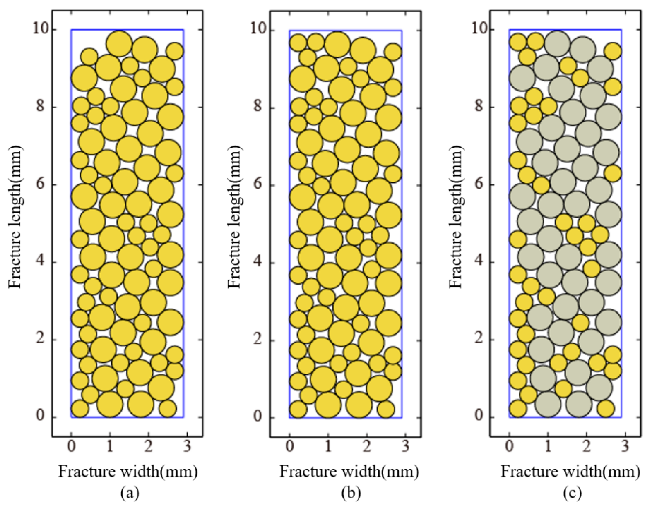
Select the diameter of the new center again as min(R^c, R^s), continue to appear, and judge whether the new circle (x_i, y_i) can continue to be filled within the boundary and on the existing circle, that is, when y_i < L_f − min(R_i)/2, it is considered that the current two-dimensional space is in a “false” full state (Figure 3a), then jump to step 4, and continue to fill a new circle with a diameter of min(R^c, R^s) in the two-dimensional space. When y_i > L_f − min(R_i)/2, it is considered that the current underlying space is “true” full (Figure 3b,c), the loop is exited, and the operation ends.

3. Numerical Calculation of Crushing Rate and Fracture Conductivity

The numerical calculation of crushing rate and fracture conductivity relies on the mechanical analysis of proppant particles. The types and particle sizes of combined proppant have inconsistent characteristics, making the numerical calculation of crushing rate and fracture conductivity more complex.

3.1. Mathematical Model and Numerical Solution for Particle Force Analysis

Taking the combination of proppant containing ceramic particles and quartz sand as an example, the combined proppant formed by fully mixing ceramsite and quartz sand in a certain proportion appears randomly according to a certain mixing proportion during computer simulation. The analysis of mechanics between particle and particle of combined proppant is very complicated, but there is also a certain law, that is, all proppant particles and particles, and particles and fracture walls are closely adjacent to each other, and there is no intersection; this is the phenomenon of suspension. Based on this rule, the mathematical expression of the combined proppant particle contact is established. At present, whether particles come into contact with one another is uncertain. The contact coefficient of the combined proppant is the same as the direct contact coefficient of multiparticle size proppant particles. For the mathematical expression of the specific contact coefficient, please refer to Guo [35], as described in the article.

In the model of the mechanics between the particle and particle as well as particle and the fracture surface, particles may either be in contact with or separate from other particles and boundaries. so any proppant needs to be listed with other particles, boundary contact, or noncontact. To determine whether to contact or not, we use the mathematical expression of multidiameter proppant particles contact in Guo [35] to make a judgment. Then, for n_p proppant particles, there are n_p equations forming an offline equation system. Therefore, the mathematical model of the mechanical relationship of the combined proppant particles is the same as the mechanical relationship model of the multidiameter proppant particles. It can be directly represented using the mathematical model of the contact between particles of multiparticle size proppants in Guo [35], as well as the interaction and reaction forces between each particle and other particles.

In the same way, the stress on the fracture boundary of the combined proppant is the same as that of the multiparticle size proppant, which can be directly expressed by the stress on the fracture boundary.

Therefore, based on the three scenarios of interparticle mechanical interactions between the combined proppant particles and the particles and between the particles and the boundary, the mechanics of combined proppant can be expressed as Equation (8):

$$AX=B$$

(8)

where A is the coefficient matrix of the linear equation system, which has the characteristics of sparse, ill-conditioned, and asymmetric. X and B are the vectors composed of the unknown and the right-hand constant term, respectively.

According to the numerical solution of the linear equation system (8) by the improved singular value decomposition method in Guo [35], the force exerted on each particle can be determined.

Different from the characteristics of single particle and multiparticle proppants, for the calculation of key parameters of combined proppant particles, it is necessary to separately consider the crushing rate and fracture conductivity of ceramic particles and quartz sand.

3.2. Calculation of Crushing Rate

The crushing rate of the proppant is the probability of crushing of the proppant particles. The combined proppant contains ceramsite and quartz sand. Considering the difference in the properties of ceramsite and quartz sand, the fracture rate of ceramsite and quartz sand must be modeled separately. First, by solving the linear equations of the mechanical relationship of the combined proppant, the force value of each proppant particle in the fracture under a given closing pressure is obtained. Then, based on the sampling curve and numerical algorithm, the fragmentation rate of each proppant particle can be calculated. The total number of particles of the combined proppant is n_p. Assuming that the number of ceramsite is n_p1 and the number of quartz sand is n_p2, the average crushing rate $\overline{{\eta }^c}$ of ceramsite is calculated from Equation (9).

$$\overline{{\eta }^c}={\displaystyle \frac{{\displaystyle \sum _{i=1}^{n_{p1}}{\eta }_i^c}}{n_{p1}}}$$

(9)

The average crushing rate of quartz sand can be calculated from Equation (10).

$$\overline{{\eta }^s}={\displaystyle \frac{{\displaystyle \sum _{j=1}^{n_{p2}}{\eta }_j^s}}{n_{p2}}}$$

(10)

Then, the overall average crushing rate can be calculated from Equation (11).

$$\overline{\eta }={\displaystyle \frac{n_{p1}\overline{{\eta }^c}+n_{p2}\overline{{\eta }^s}}{n_{p1}+n_{p2}}}$$

(11)

where $\overline{\eta }$ is the average crushing coefficient of combined proppant (dimensionless). $\overline{{\eta }^c}$ is the average crushing coefficient of ceramsite (dimensionless). $\overline{{\eta }^s}$ is the average crushing coefficient of quartz sand (dimensionless). ${\eta }_i^c$ is ceramsite crushing coefficient (dimensionless). ${\eta }_j^s$ is the crushing coefficient of quartz sand (dimensionless). n_p is the total number of combined proppant particles (dimensionless). n_p1 is the total number of ceramsites (dimensionless). n_p2 is the total number of quartz sand (dimensionless). i is the number of ceramsite particles, i = 1, 2, …, n_p1. j is the number of quartz sand particles, j = 1, 2, …, n_p2.

3.3. Calculation of Fracture Conductivity

The fracture conductivity of combined proppant is equal to the permeability multiplied by the fracture width. Considering the dimensional relationship, the fracture conductivity can be calculated from Equation (12).

$$C_f=0.1K_f{w}_f$$

(12)

where C_f is the fracture conductivity supported by the combined proppant, μm²·cm. K_f is the fracture permeability of the combined proppant, μm². w_f is the fracture width (mm).

(1)

Calculation model of permeability

According to the Kozeny–Garman equation, combined with the combined proppant particles, the two particle sizes are mixed in different proportions, and the fracture permeability K of the combined proppant particles can be calculated from Equation (13).

$$K={\displaystyle \frac{{\overline{R}}_p^2}{180}}{\displaystyle \frac{{\varphi }^3}{{(1-\varphi )}^2}}$$

(13)

Among them, K is the fracture permeability, μm². ϕ is the porosity (dimensionless). ${\overline{R}}_p$ is the average particle size of the combined proppant (mm), and it can be calculated from Equation (14).

$${\overline{R}}_p={\displaystyle \frac{n_{p1}{R}^c+n_{p2}{R}^s}{n_{p1}+n_{p2}}}$$

(14)

Among them, n_p1 is the total number of ceramsites (dimensionless). n_p2 is the total number of quartz sand (dimensionless). R^c is the particle size of ceramsite (mm). R^s is the particle size of quartz sand (mm).

(2)

Calculation model of porosity

The calculation idea of fracture porosity of combined proppant is similar to that of multiparticle size proppant particles and proppant with single particle size. The fracture porosity is correlated with the ratio of the total fracture area to the area occupied by proppant particles. by the proppant particles. The degree is correlated with the proppant crushing rate.

(a)

The case where none of the composite proppant particles are broken η = 0

When no closure pressure is applied to the fracture, the ceramsite and quartz sand in the fracture are not broken. Fracture porosity refers to the fraction of the total fracture area occupied by pores. Based on the characteristics of the combined proppant particles, the fracture porosity can be calculated from Equation (15).

$$\varphi ={\displaystyle \frac{w_f{L}_f-{\displaystyle \sum _{i=1}^{n_{p1}}\left(\frac{1}{4}\pi {(R_i^c)}^2\right)-{\displaystyle \sum _{j=1}^{n_{p2}}\left(\frac{1}{4}{(\pi R_j^s)}^2\right)}}}{w_f{L}_f}}$$

(15)

(b)

The case of combined proppant particle crushing rate η ≠ 0

When the closing pressure was applied, the ceramsite and quartz sand in the fractures were broken to varying degrees. The overall performance of quartz sand is worse than that of ceramsite. Under the same closing pressure, the crushing rate of quartz sand is higher than that of ceramsite. After the proppant is broken, the tiny particles will fill the pores between the unbroken proppant particles, and the fracture shrinks and the fracture width decreases. Based on the principle of mass conservation, after the proppant particles are broken, the area occupied by the proppant particles remains unchanged, and the formula of the calculating fracture porosity changes from Equation (15) to Equation (16).

$$\varphi \text{'}={\displaystyle \frac{\left(w_f{L}_f-A_c\right)-{\displaystyle \sum _{i=1}^{n_{p1}}\left(\frac{1}{4}\pi {(R_i^c)}^2\right)-{\displaystyle \sum _{j=1}^{n_{p2}}\left(\frac{1}{4}\pi {(R_j^s)}^2\right)}}}{w_f{L}_f-A_c}}$$

(16)

where A_c is the total area where the combined proppant particles are broken, which can be calculated from Equation (17).

$$A_c={\displaystyle \sum _{i=1}^{n_{p1}}\left(\frac{1}{4}\pi {(R_i^c)}^2{\eta }_i^c\right)}+{\displaystyle \sum _{j=1}^{n_{p2}}\left(\frac{1}{4}\pi {(R_j^s)}^2{\eta }_j^s\right)}$$

(17)

Substituting Equation (17) into Equation (16), the calculation formula of fracture porosity can be calculated from Equation (18).

$$\varphi \text{'}=1-{\displaystyle \frac{{\displaystyle \sum _{i=1}^{n_{p1}}\left(\pi {(R_i^c)}^2\right)}+{\displaystyle \sum _{j=1}^{n_{p2}}\left(\pi {(R_j^s)}^2\right)}}{4w_f{L}_f-{\displaystyle \sum _{i=1}^{n_{p1}}\left(\pi {(R_i^c)}^2{\eta }_i^c\right)}-{\displaystyle \sum _{j=1}^{n_{p2}}\left(\pi {(R_j^s)}^2{\eta }_j^s\right)}}}$$

(18)

At the same time, the fracture width becomes smaller under the closure pressure of the hydraulic fracture. The formula for calculating the fracture width can be calculated from Equation (19).

$$w{\text{'}}_f=w_f-{\displaystyle \frac{{\displaystyle \sum _{i=1}^{n_{p1}}\left(\pi {(R_i^c)}^2{\eta }_i^c\right)}+{\displaystyle \sum _{j=1}^{n_{p2}}\left(\pi {(R_j^s)}^2{\eta }_j^s\right)}}{4L_f}}$$

(19)

Among them, ϕ is the porosity when the proppant is not broken (dimensionless). ϕ’ is the porosity when the proppant is broken (dimensionless). A_c is the total area of the combined proppant particles broken (mm²). w_f is the proppant fracture width when the proppant does not break (mm). w’_f is the crack width after the proppant is broken (mm). L_f is the crack length (mm). n_p1 is the quantity of ceramsite (dimensionless). n_p2 is the quantity of quartz sand (dimensionless). i is the number of ceramsite particles, i = 1, 2, …, n_p1. j is the number of quartz sand particles, j = 1, 2, …, n_p2.

(3)

Calculation model of fracture conductivity

For the calculation model of fracture conductivity of combined proppant, substitute Equation (18) into Equation (13) to obtain fracture permeability, and then combine Equation (19) to obtain the calculation formula (20) for the fracture conductivity of the combined proppant.

$$C_f={\displaystyle \frac{1}{7200}}{\left({\displaystyle \frac{{\displaystyle \sum _{i=1}^{n_{p1}}{R}_i^c}}{n_{p1}}}+{\displaystyle \frac{{\displaystyle \sum _{j=1}^{n_{p2}}{R}_j^s}}{n_{p2}}}\right)}^2{\displaystyle \frac{{\left(4w_f{L}_f-{\displaystyle \sum _{i=1}^{n_{p1}}\left(\pi {(R_i^c)}^2\right)}-{\displaystyle \sum _{j=1}^{n_{p2}}\left(\pi {(R_j^s)}^2\right)}-{\displaystyle \sum _{i=1}^{n_{p1}}\left(\pi {(R_i^c)}^2{\eta }_i^c\right)}-{\displaystyle \sum _{j=1}^{n_{p2}}\left(\pi {(R_j^s)}^2{\eta }_j^s\right)}\right)}^3}{4L_f{\left({\displaystyle \sum _{i=1}^{n_{p1}}\left(\pi {(R_i^c)}^2\right)}+{\displaystyle \sum _{j=1}^{n_{p2}}\left(\pi {(R_j^s)}^2\right)}\right)}^2}}$$

(20)

4. Calculation Results and Analysis

According to the characteristics, which means that the performance, the particle size, and the proportion may be different of the combined proppant, the 20/40 mesh LZ sand, 20/40 mesh XY ceramsite, and 30/50 mesh XY ceramics, which are widely used in China, are selected. As the experimental material, and according to the standard test procedures recommended by SY/T 5108-2006 [43], SY/T 6302-2009 [44], and API RP56 [45], the crushing rate and fracture conductivity of the combined proppant were tested and calculated.

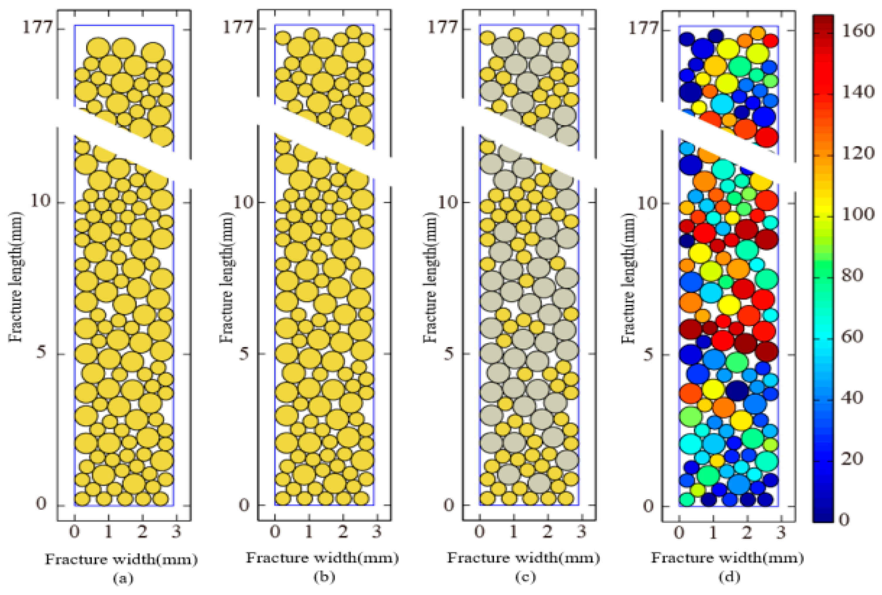
4.1. Particle Arrangement and Force Simulation

For the combined proppant with the same particle size and the same proportion, we select 20/40 mesh LZ sand and 20/40 mesh XY ceramsite, and mix them randomly according to the ratio of 1:1. For the combined proppant, we selected combinations of varying particle sizes; specifically, an equal proportion mix of 20/40 mesh LZ sand and 30/50 mesh XY ceramic particles are used in the experiment, and are mixed randomly according to the ratio of 1:1. The laying concentration of the two types of combined proppant is 5 kg/m², and the closing pressure is 10~60 MPa.

The diameter of the proppant crushing chamber is 40.5 mm, the length of the proppant diversion chamber is 177.8 mm, and when the proppant concentration is set to 5 kg/m² (crack width is about 2.9 mm), the particle size of the combined proppant is randomly generated according to Formula (1). We simulate the arrangement and force of two types of combined proppant particles, as shown in Figure 4, Figure 5, Figure 6 and Figure 7.

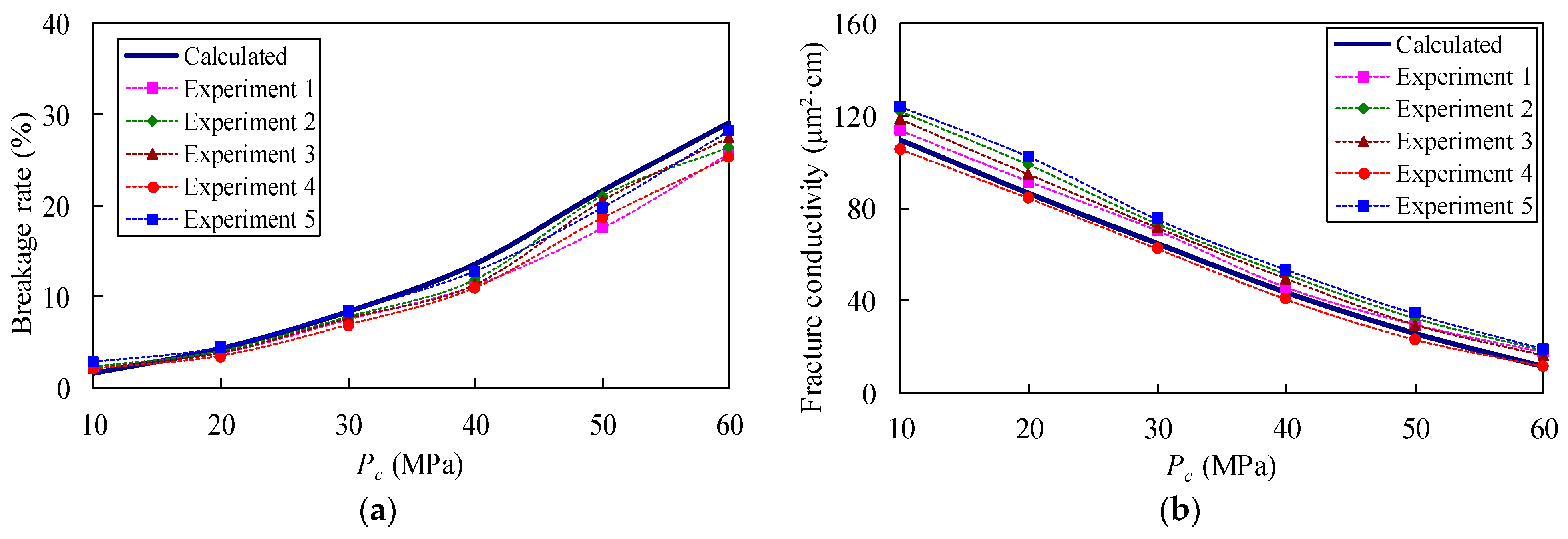
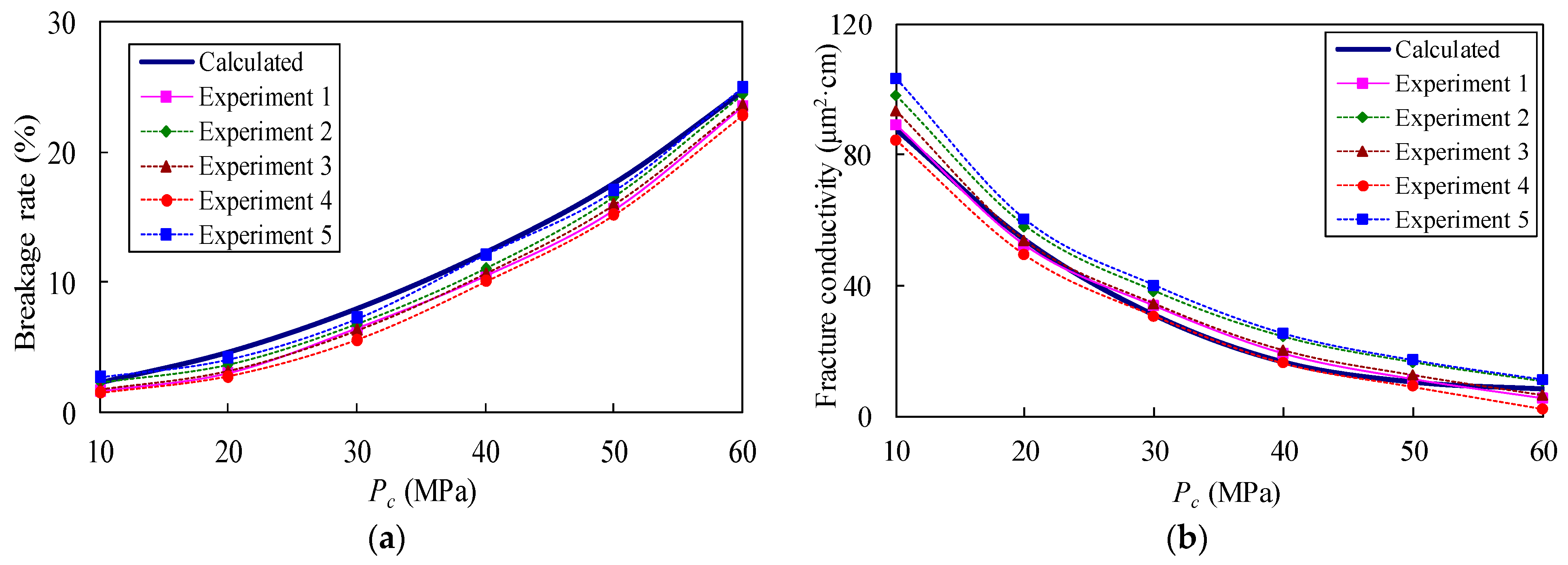
4.2. Comparison between Calculations and Experiments

Combination proppants with the same particle size and proportion, as well as those with different particle sizes and proportions, adopt the above combination mode. In the simulation and experiment of proppants with the same particle size but different ratios, 20/40 mesh LZ sand and 20/40 mesh XY ceramic particles were selected and randomly mixed in five different ratios of 1:1, 1:1.2, 1:1.5, 1:1.8, and 1:2. The laying concentration of the combined proppant was 5 kg/m², and the closing pressure was 10–60 MPa. Numerical solutions and experiments were conducted on three different types of composite proppants to obtain their crushing rate and fracture conductivity. The comparison between the experimental and calculated results is shown in Figure 8, Figure 9 and Figure 10.

It can be seen from Figure 8, Figure 9 and Figure 10 that the calculated values of both the crushing rate and fracture conductivity of the combined proppant are basically consistent with the experimental values, and the difference between the calculated values and the experimental values is small, which verifies the effectiveness of the numerical solution method proposed in this paper.

4.3. Discussion of Calculation Results

The test results of the same particle size and proportion combination proppant (20/40 mesh LZ sand and 20/40 mesh XY ceramic particles, randomly mixed in a 1:1 ratio) show that under a closing pressure of 10–60 MPa, the maximum error between the calculated crushing rate of the combined proppant model and the experimental value is 29.50%, the minimum error is 9.08%, and the average error is 14.51%. The consistency between the calculated crushing rate of the model and the experimental values reached 85.49%. Under a closing pressure of 10–60 MPa, the maximum error between the calculated fracture conductivity value of the combined proppant model and the experimental value is 31.59%, the minimum error is 6.12%, and the average error is 12.98%. The coincidence rate between the calculated fracture conductivity value of the model and the experimental value reached 87.02%.

The test results of different particle sizes and proportions of combined proppants (20/40 mesh LZ sand and 30/50 mesh XY ceramic particles, randomly mixed in a 1:1 ratio) show that under a closing pressure of 10–60 MPa, the maximum error between the calculated crushing rate of the combined proppant model and the experimental value is 39.11%, the minimum error is 3.31%, and the average error is 17.66%. The consistency between the calculated crushing rate of the model and the experimental values reached 82.34%. Under a closing pressure of 10–60 MPa, the maximum error between the calculated fracture conductivity value of the combined proppant model and the experimental value is 20.02%, the minimum error is 1.70%, and the average error is 13.24%. The coincidence rate between the fracture conductivity calculated by the model and the experimental values reached 86.76%.

The test results for combined proppants with the same particle size but different proportions (20/40 mesh LZ sand and 20/40 mesh XY ceramic particles, randomly mixed in five different ratios of 1:1, 1:1.2, 1:1.5, 1:1.8, and 1:2, shown in Figure 10) show that under a closing pressure of 10–60 MPa, as the proportion of ceramic particles increases, the crushing rate of the combination proppant decreases, and the crack conductivity of the combination proppant increases. It was proven that the more proportion of high-performance proppants there are, the greater fracture conductivity can be provided.

From Figure 8, Figure 9 and Figure 10, it can also be seen that quartz sand can meet the performance requirements of proppants when the closure pressure of the reservoir is below 40 MPa. If the closing pressure exceeds 60 MPa, ceramsite needs to be selected to meet the performance requirements of the proppant, and when the closing pressure is between 40 and 60 MPa, the combination of quartz sand and ceramic particles can balance performance and cost. In addition, the convergence of the computational model is also discussed, as shown in Figure 11.

Figure 11 shows the relationship between the cumulative average and total average of the fracture conductivity of a combination proppant with the same particle size and proportion (20/40 mesh LZ sand and 20/40 mesh XY ceramic particles, randomly mixed in a 1:1 ratio). After six simulations, the discrepancy between the cumulative mean and the overall mean drops below 3%. Upon reaching 21 simulations, this difference tightens to less than 1%. As the number of simulations rises, the error progressively diminishes towards zero. Therefore, setting the simulation frequency to 21 can meet the accuracy requirements.

5. Application and Effect Analysis

Combination proppants have been applied in a tight oil block of XJ in China. The oil-bearing area of this block is 140.6 km², with a controlled reserve of nearly 100 million tons. The resources are relatively abundant and the potential is enormous. The closing pressure of the tight oil reservoir is 45~55 MPa, and it is expected to deploy 160 horizontal wells. The number of fracturing sections for these horizontal wells is roughly the same, all of which are 7–9 sections. Quartz sand has low cost (XJ commonly uses LZ sand with a cost of USD 169/square meter), but it cannot meet performance requirements. Ceramic particles have good performance, but the cost is too high (XJ commonly uses XY ceramic particles with a cost of USD 530/square meter). The contradiction between cost and performance is one of the major bottlenecks and expected solutions to achieve the development of tight oil benefits.

It is not feasible to simply use quartz sand for hydraulic fracturing in response to the pressure situation of XJ tight oil reservoirs. Using high-performance ceramic particles is the main choice for onsite hydraulic fracturing. In order to further reduce production costs and ensure sufficient fracture conductivity within the reservoir, hydraulic fracturing tests were conducted onsite using sand addition methods such as excessive all-quartz sand and combined proppant. Among them, excessive all-quartz sand means all-quartz sand which is 1.5 to 2.5 times the normal amount, and can improve the fracture conductivity through high laying concentration. This is an experiment where a single-quartz sand or ceramic particle cannot meet the onsite needs.

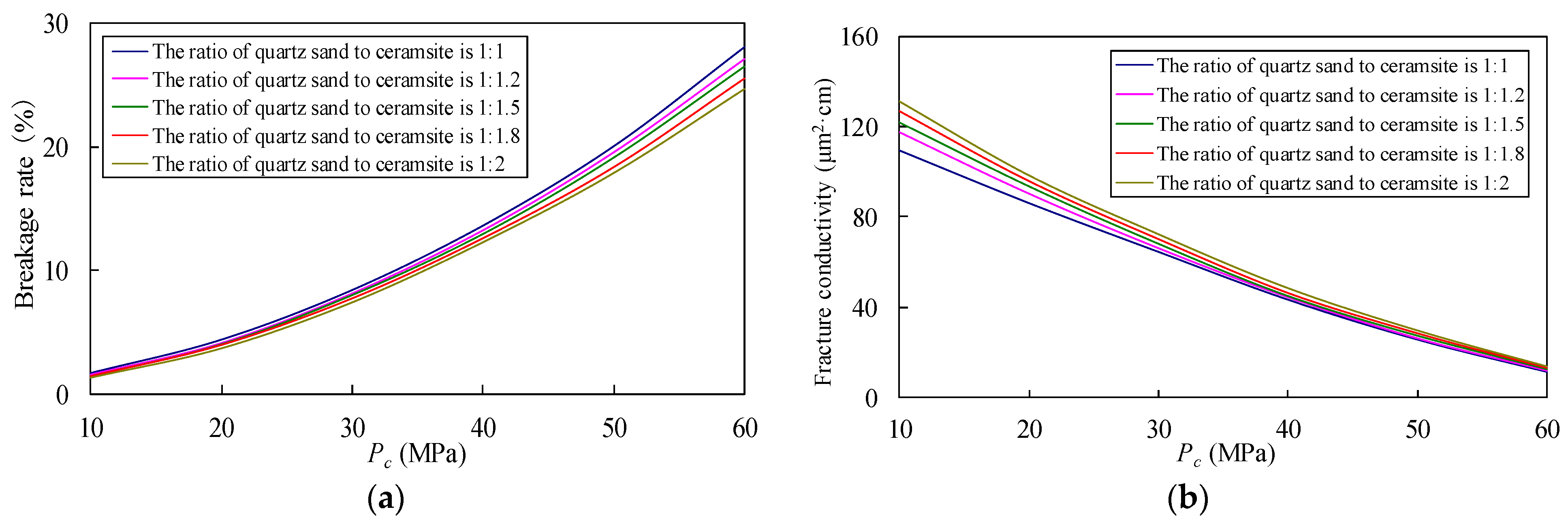
5.1. Proportional Optimization

The optimal mixing ratio of ceramic particles and quartz sand in combined proppants is an important guarantee for the successful construction and post-fracturing production of onsite fracturing wells. In order to facilitate onsite hydraulic fracturing construction and ensure fracture conductivity, the combined proppant process is optimized and the combined proppant construction process is designed.

Using net present value (NPV) to reflect the difference between the present value of future cash flows and the present value of investments in the target block’s horizontal wells, the net present value of fracturing can be expressed by Equation (21).

$$NPV=P_{af}-P_{bf}-C_P$$

(21)

Among them, NPV is the net present value (USD). P_af is the present value after fracturing (USD). P_bf is the present value without fracturing (USD). C_P is the cost of fracturing (USD).

We establish the objective function to maximize NPV as Equation (22).

$$\max NPV(R_D,V_l,V_p,\alpha ,x)$$

(22)

Among them, R_D is the construction displacement (m³/min). V_l is the total amount of fracturing fluid (m³). V_p is the total amount of proppant (m³). α is the sand ratio, %. x is the proportion of quartz sand (dimensionless). D, l, and p are subscripts, representing displacement, fracturing fluid volume, and proppant volume, respectively.

In the above optimization model (22), firstly, the optimal construction displacement, fracturing fluid volume, proppant volume, and sand ratio in different pumping stages are calculated through complex external circulation. Then, through internal circulation, the optimal proportion of quartz sand in the composite proppant is calculated. Among them, the objective of internal circulation optimization is the NPV of the objective function regarding the proportion x of quartz sand, as shown below.

$$\max NPV(x)$$

(23)

According to the established optimization objective function (23), the maximum value of NPV is obtained by searching for the global optimal solution. By drawing the relationship curve between NPV and the proportion of quartz sand x, we find the extreme point of NPV and obtain the optimal proportion of quartz sand.

As shown in Figure 12, according to the curve relationship between NPV and quartz sand proportion x, it can be concluded that when the quartz sand proportion x is 1.0231, the NPV (x) value is maximum. Therefore, it is determined that the mixing ratio of 20/40 mesh LZ sand and 20/40 mesh XY ceramic particles in the combined proppant is 1:1.

5.2. Onsite Construction Technology

Assuming a fracture length of approximately 164 m and a fracture height of approximately 30 m (the actual oil layer thickness is approximately 10 m), according to the placement of proppant inside the fracture, the fracture width at the tip of the fracture is very small, and the proppant cannot reach it. This is the pure liquid area of the fracturing fluid. The use of a 1:1 sand addition method for combined proppants cannot meet the fracture conductivity. In order to transport proppant particles to the far end of the fracture as much as possible, a certain volume of small-particle-size proppant should be pumped first during the carrying fluid stage. Therefore, we add 10% of 30/50 mesh small-particle-size ceramic particles in the initial stage of fracturing. The proppant scheme has been adjusted to a combination of 10% small ceramic particles (XY ceramic particles 30/50) and 90% combined proppant (20/40 mesh LZ sand mixed with 20/40 mesh XY ceramic particles in a 1:1 ratio). In this way, not only can the small-particle-size proppant be placed as much as possible at the tip of the fracture, but it can also ensure the fracture conductivity.

The proppants used in onsite hydraulic fracturing construction include 40/70 mesh LZ sand (pad fluid stage), 20/40 mesh LZ sand, 30/50 mesh XY ceramic particles, and 20/40 mesh XY ceramic particles.

The sand addition steps for onsite hydraulic fracturing were designed, as shown in Figure 13. The device mainly includes four sand boxes and six funnels, which can flexibly adjust the sand storage space. The first sand box contains 40/70 mesh LZ sand, the second sand box contains 30/50 mesh small XY ceramic particles, while the third and fourth sand boxes contain LZ sand and XY ceramic particles, respectively.

The specific construction steps for composite proppants are as follows.

(1)

As shown in Figure 13, add 40/70 mesh LZ sand (usually 2 m³) to the No. 1 sand box to polish the fracture during the pre-liquid stage. Add 4 m³ of 30/50 mesh XY ceramic particles to the No. 2 sand box. Add 21.8 m³ of 20/40 mesh LZ sand to the No.3 sand box. Add 21.8 m³ of 20/40 mesh XY ceramic particles to the No. 4 sand box.

(2)

According to the designed pumping program, first open funnel ① and inject 40/70 mesh LZ sand during the pre-liquid stage. During the carrying-fluid stage, open funnel ② and inject small XY ceramic particles into sand box 2. After all the small diameter XY ceramic particles in box 2 are pumped in, immediately open funnels ③, ④, ⑤, and ⑥, and mix 20/40 mesh LZ sand with 20/40 mesh XY ceramic particles in a 1:1 ratio for pumping construction until the construction is completed.

5.3. Application Effects and Comparison

In a certain block of XJ tight oil in China, 40 horizontal wells were constructed using the method of adding sand with all ceramic particles, 5 horizontal wells were constructed using an excessive all-quartz sand, and 3 horizontal wells were constructed using a combination proppant (20/40 mesh LZ sand and 20/40 mesh XY ceramic particles mixed in a 1:1 ratio). These horizontal wells have roughly the same number of fracturing sections, all ranging from 7 to 9. A comparative analysis was conducted on the cost and oil production of proppants, as shown in

Table 1. The average cost and economic benefits of each section for different sand addition methods.

Well	Proppant	Average Proppant Volume (m3)	Average Proppant Cost (USD)	Average Daily Production (t/d)	Cost Reduction (%)	Production Increment (%)
A	All ceramsite	73.62	38,996	15.47	/	/
B	Excessive all-quartz sand	149.88	25,373	5.61	34.95	−63.72
C	Combined proppant	66.67	25,296	17.66	40.25	14.10

.

Under the same reservoir conditions as XJ tight oil, there are a total of 40 wells using the all ceramsite sand addition method, with a proppant volume of 57.94–11.65 m³ and an average proppant volume of 73.62 m³. The proppant cost is USD 30,699–60,200, with an average proppant cost of USD 38,996 and a daily oil production of 1.77–34.72 t/d, and an average daily oil production of 15.47 t/d.

There are 5 wells using the method of adding excessive all-quartz sand, with a proppant volume of 135.29–166.26 m³ and an average proppant volume of 149.88 m³. The cost of proppant is USD 22,897–28,139, and the average proppant cost is USD 25,373. Compared with all ceramsite, the average proppant cost is reduced by 34.95%. The daily oil production is 3.28–9.10 t/d, with an average daily oil production of 5.61 t/d. Compared with all ceramsite, the average daily oil production is reduced by 63.72%. Although excessive all-quartz sand reduces production costs, compared to ceramic particles, quartz sand has poor performance, high crushing rate, and low fracture conductivity, resulting in low daily production of tight oil.

Three wells were constructed using a combined proppant composed of ceramic particles and quartz sand mixed in a 1:1 ratio. The proppant volume is 50–80 m³, with an average proppant volume of 66.67 m³. The proppant cost is USD 1748–27,960, and the average proppant cost is USD 23,296. Compared with all ceramsite, the average proppant cost decreased by 40.25%, and, compared with excessive all-quartz sand, the average proppant cost decreased by 8.15%. The daily oil production is 13.68–21.12 t/d, with an average daily oil production of 17.66 t/d. Compared with all ceramsite, the average daily oil production has increased by 14.10%. It has been proven that the use of combined proppants can not only greatly reduce production costs, but also effectively increase the daily production of tight oil.

We selected fracturing wells with the same reservoir geological conditions in the target block for analysis. There were four wells using all ceramsite proppant for hydraulic fracturing, represented by A1, A2, A3, A4. Two wells were subjected to hydraulic fracturing using excessive all-quartz sand proppant and combined proppant, respectively represented by B1 and C1.

The simultaneous production curve of the excessive all-quartz sand test well B1 is shown in Figure 14. From 2019 to 2020, the cumulative oil production was 1995.8 tons, with a maximum oil production of 12.2 t/d and an average daily oil production of 5.89 t/d.

Compared to all ceramsite, although the cost of excessive all-quartz sand decreased by 34.95%, the average daily oil production decreased by 63.72%. At the same time, excessive all-quartz sand increases the sand volume by 100% on the basis of the original sand volume, which will inevitably increase the sand-carrying fluid volume by 100%, greatly increasing the total cost of fracturing fluid.

The test well used a combination proppant and produced continuously for 339 days after fracturing. The production data are shown in Figure 14. The maximum daily oil production is 31.3 t/d, the average daily oil production is 18.17 t/d, and the cumulative oil production is 6158.2 t, achieving ideal fracturing effect. By comparing the construction costs and production effects of all ceramsite and excessive all-quartz sand from adjacent wells, it has been proven that combined proppants can balance performance and price, and are an economically effective method for hydraulic fracturing of special reservoirs.

6. Conclusions

The main objective of this research was to establish a computer simulation method for combined proppant, in order to select the optimal proppant material and optimize the combination of different proppant types, and solve the contradiction between cost and performance of proppants. The results can be used for optimizing proppant schemes in the hydraulic fracturing process of unconventional oil and gas. The following conclusions are summarized.

(1)

By studying the microscopic arrangement structure of combined proppant particles and based on the randomness and determinacy phenomena in the process of proppant particle arrangement, corresponding solutions were proposed, and computer simulation of combined proppant particles was achieved.

(2)

Considering the possible differences in performance, particle size, and proportion of combined proppants, a crushing rate calculation model for combined proppants was established.

(3)

A permeability model for composite proppants was established based on the Kozeny–Garman equation. A mathematical model for the crack conductivity of composite proppant particles was established based on the actual situation of fracture width reduction after particle crushing.

(4)

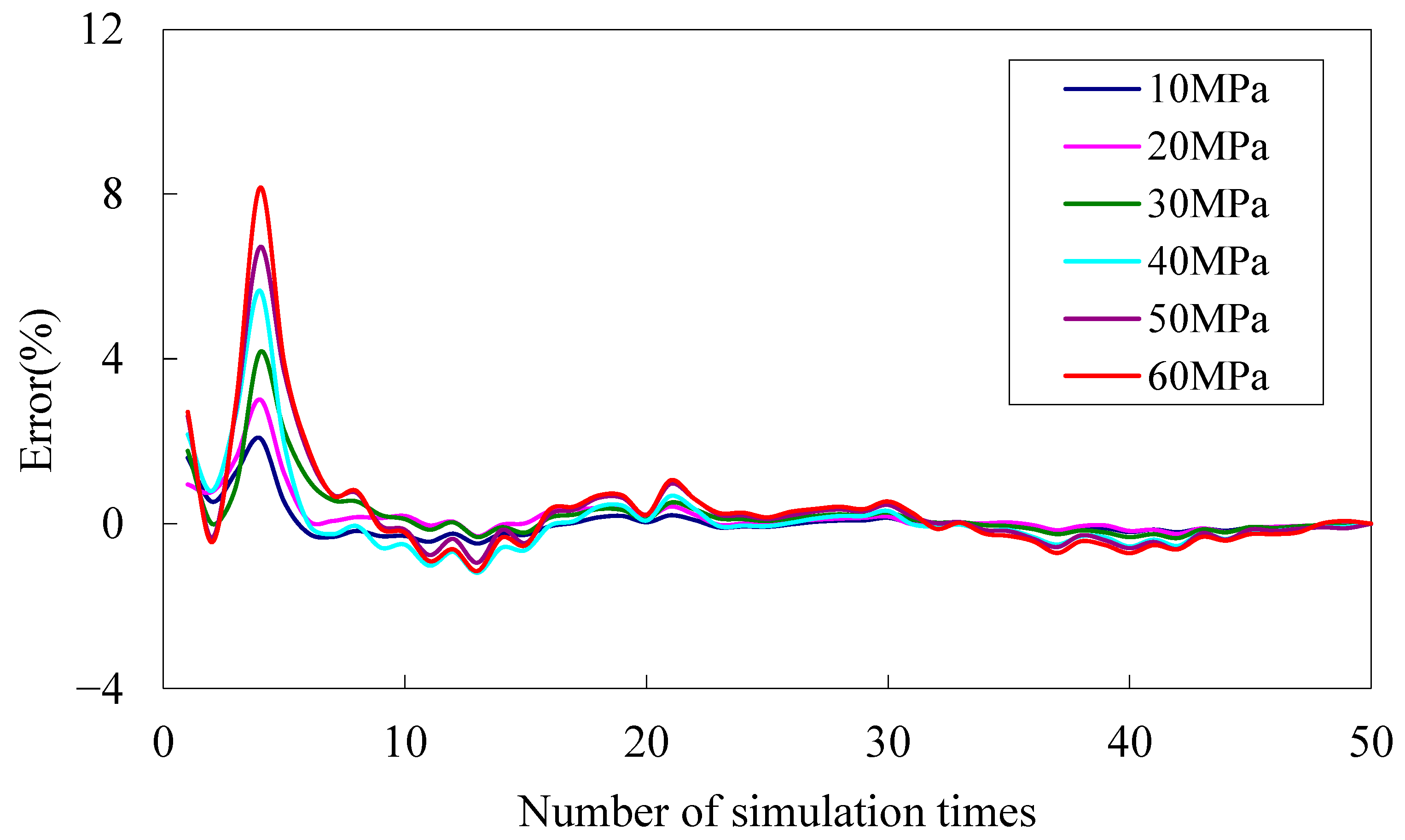
The calculation results of the crushing rate of combined proppants with the same particle size and proportion, as well as different particle sizes and proportions, show that under a closing pressure of 10–60 MPa, the crushing rate and fracture conductivity values calculated by the model are in agreement with the experimental values by more than 80%.

(5)

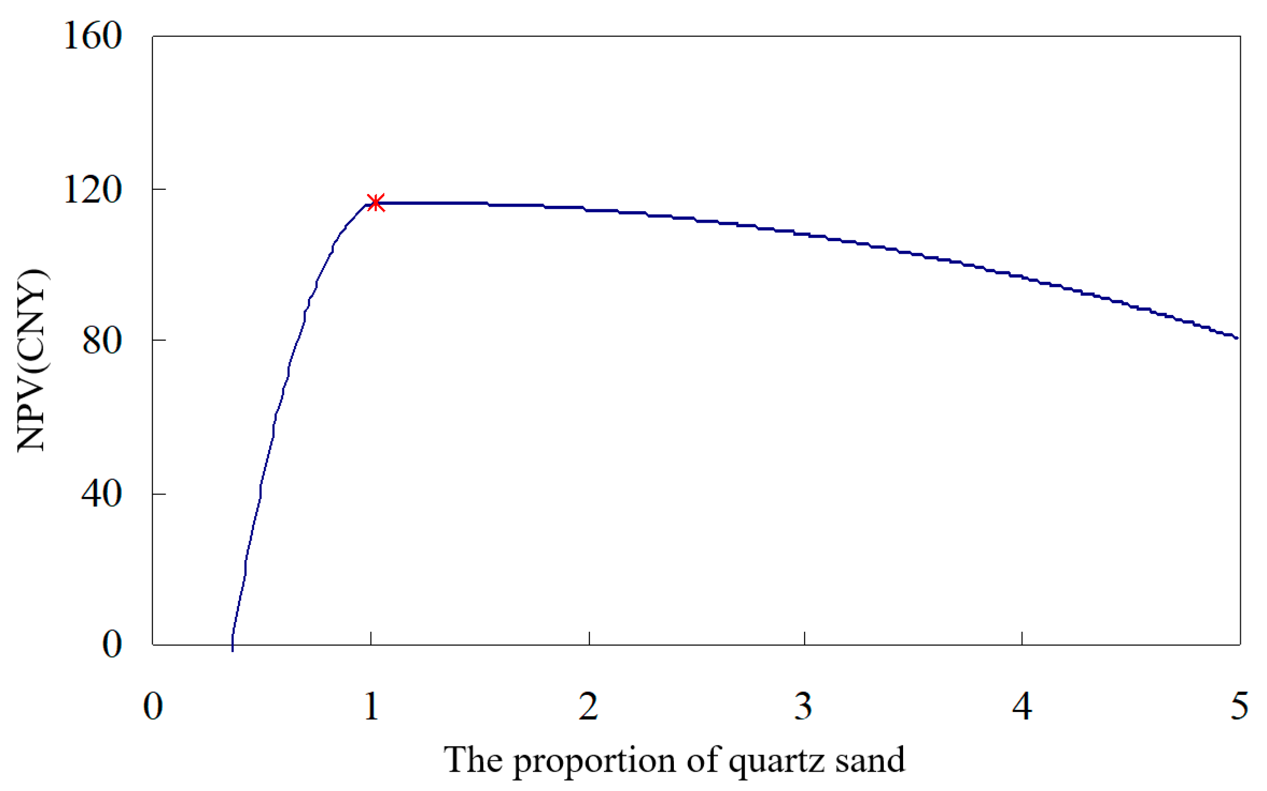
The calculation results of combined proppants with the same particle size but different proportions indicate that as the proportion of ceramic increases, the fracture conductivity of the combined proppant becomes greater.

(6)

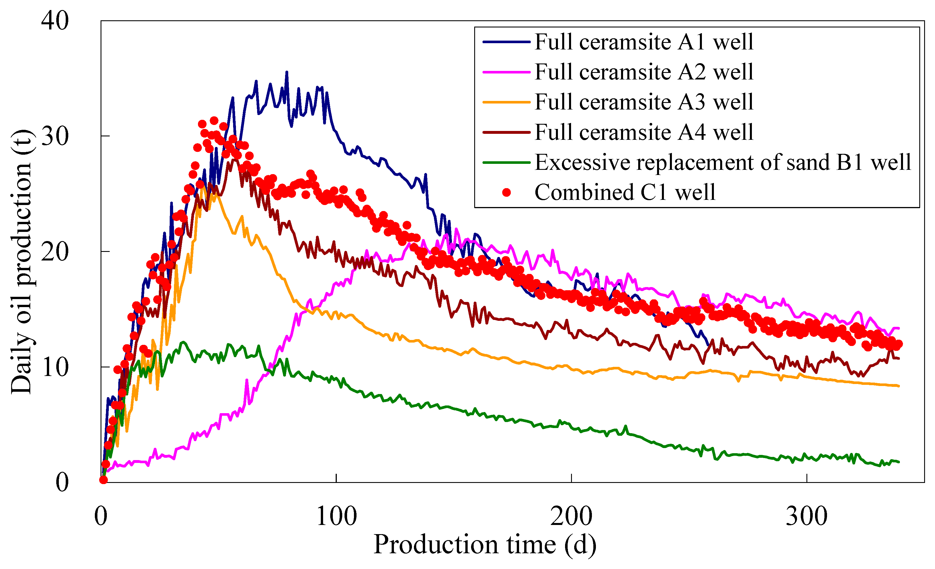
Applied to the fracturing of target block reservoirs with a closed pressure of 45 MPa~55 MPa, the results showed that the combination proppant effectively reduced the proppant cost by about 40.25%, and the oil production achieved the expected results. The daily oil production increased by about 14.10% compared to the production well with all ceramsite. Practice has proven the rationality and effectiveness of combined proppants.

Based on the comprehensive evaluation of the methods and results of this research, the following future research directions are proposed.

(1)

In this research, it is assumed that the proppant particles are in a static laying state. Multiple methods and disciplines such as fluid dynamics theory can be combined to study the key performance parameters of proppant, so as to achieve the purpose of dynamic simulation.

(2)

Considering the sphericity of proppant particles and actual reservoir characteristics, additional studies on the embedding and deformation of proppant are important directions.

(3)

This article studies the computer simulation of proppants and the calculation of key parameters from a two-dimensional perspective. Carrying out three-dimensional simulation and numerical modeling of proppant particles is an important direction for future work.

References

1. Wang, H.Y. Hydraulic fracture propagation in naturally fractured reservoirs, complex fracture or fracture networks. J. Nat. Gas Sci. Eng. 2019, 68, 102911. [Google Scholar] [CrossRef]
2. Guo, Z.X.; Chen, Y.Y.; Zhou, X.; Zeng, F.H. Inversing fracture parameters using early-time production data for fractured wells. Inverse Probl. Sci. 2020, 28, 674–694. [Google Scholar] [CrossRef]
3. Keshavarz, A.; Yang, Y.L.; Badalyan, A.; Johnson, R.; Bedrikovetsky, P. Laboratory-based mathematical modelling of graded proppant injection in CBM reservoirs. Int. J. Coal Geol. 2014, 136, 1–16. [Google Scholar] [CrossRef]
4. Osholake, T.; Wang, J.Y.L.; Ertekin, T. Factors affecting hydraulically fractured well performance in the marcellus shale gas reservoirs. J. Energ. Resour. Technol.-Asme 2013, 135, 013402. [Google Scholar] [CrossRef]
5. Ren, J.J.; Gao, Y.Y.; Zheng, Q.; Wang, D.L. Pressure transient analysis for a finite-conductivity fractured vertical well near a leaky fault in anisotropic linear composite reservoirs. J. Energy Resour. Technol.-ASME 2020, 142, 073002. [Google Scholar] [CrossRef]
6. Wu, J.F.; He, Y.T.; Zeng, B.; Huang, H.Y.; Gui, J.C.; Guo, Y.T. Numerical simulation study on the ultimate injection concentration and injection strategy of a proppant in hydraulic fracturing. Energy Fuels 2024, 12, 2296–2598. [Google Scholar] [CrossRef]
7. Bai, Z.F.; Li, M.Z.; Li, J.Y.; Li, C.X. Effect of proppant injection condition on fracture network structure and conductivity. Energy Sci. Eng. 2024, 2024, 1–19. [Google Scholar] [CrossRef]
8. Hou, L.; Elsworth, D.; Zhang, F.S.; Wang, Z.Y.; Zhang, J.B. Evaluation of proppant injection based on a data-driven approach integrating numerical and ensemble learning models. Energy 2022, 264, 126122. [Google Scholar] [CrossRef]
9. Zhang, B.; Cui, X.Y.; Wang, L.J.; Fu, X.D. Rock fracture response exposed to hydraulic fracturing: Insight into the effect of injection rate on aperture pattern. Adv. Mater. Sci. Eng. 2022, 2022, 9431143. [Google Scholar] [CrossRef]
10. Roostaei, M.; Nouri, A.; Fattahpour, V.; Chan, D. Coupled hydraulic fracture and proppant transport simulation. Energies 2020, 13, 2822. [Google Scholar] [CrossRef]
11. Zhang, Z.P.; Zhang, S.C.; Ma, X.F.; Guo, T.K.; Zhang, W.Z.; Zou, Y.S. Experimental and numerical study on proppant transport in a complex fracture system. Energies 2020, 13, 6290. [Google Scholar] [CrossRef]
12. Barboza, B.R.; Chen, B.; Li, C.F. A review on proppant transport modelling. J. Petrol. Sci. Eng. 2021, 204, 108753. [Google Scholar] [CrossRef]
13. Liu, G.L.; Chen, S.; Xu, H.X.; Zhou, F.J.; Sun, H.; Li, H.; Wang, Z.W.; Li, X.W.; Song, K.P.; Rui, Z.H.; et al. Experimental investigation on proppant transport behavior in hydraulic fractures of tight oil and gas reservoir. Geofluids 2022, 2022, 1385922. [Google Scholar] [CrossRef]
14. Li, J.; Han, X.; He, S.Y.; Wu, M.Y.; Huang, X.; Li, N.Y. Effect of proppant sizes and injection modes on proppant transportation and distribution in the tortuous fracture model. Particuology 2024, 84, 261–280. [Google Scholar] [CrossRef]
15. Xiong, P.Q.; Sun, L.; Wu, F.P.; Song, A.L.; Zhou, J.Y.; Li, X.G.; Li, H.Z. Simulation and solution of a proppant migration and sedimentation model for hydraulically fractured inhomogeneously wide fractures. Energy Explor. Exploit. 2024, 42, 1315–1343. [Google Scholar]
16. Kaufmann, R.; Connelly, C. Oil price regimes and their role in price diversions from market fundamentals. Nat. Energy 2020, 5, 141–149. [Google Scholar] [CrossRef]
17. Jang, P.Y.; Beruvides, M.G. Time-varying influences of oil-producing countries on global oil price. Energies 2020, 13, 1404. [Google Scholar] [CrossRef]
18. Zhu, K.; Guo, D.L.; Zeng, X.H.; Li, S.G.; Liu, C.Q. Proppant flowback control in coal bed methane wells, experimental study and field application. Int. J. Oil Gas Coal Technol. 2014, 7, 189–202. [Google Scholar] [CrossRef]
19. Hou, T.F.; Zhang, S.C.; Ma, X.F.; Shao, J.J.; He, Y.A.; Lv, X.R.; Han, J.Y. Experimental and theoretical study of fracture conductivity with heterogeneous proppant placement. J. Nat. Gas Sci. Eng. 2017, 37, 449–461. [Google Scholar] [CrossRef]
20. Wang, L.; Wen, H. Experimental investigation on the factors affecting proppant flowback performance. J. Energy Resour. Technol.-ASME 2020, 142, 053001. [Google Scholar] [CrossRef]
21. Wen, Q.Z. Experimental investigation of propped fracture network conductivity in naturally fractured shale reservoirs. In Proceedings of the SPE Annual Technical Conference and Exhibition, New Orleans, LA, USA, 30 September–2 October 2013. [Google Scholar]
22. McDaniel, G.A.; Abbott, J.; Mueller, F.; Anwar, A.M.; Pavlova, S.; Nevvonen, O.; Parias, T.; Alary, J. Changing the shape of fracturing, new proppant improves fracture conductivity. In Proceedings of the SPE Annual Technical Conference and Exhibition, Florence, Italy, 20–22 September 2010. [Google Scholar]
23. Chang, O.; Kinzel, M.; Dilmore, R.; Wang, J.Y.L. Physics of proppant transport through hydraulic fracture network. J. Energ. Resour. Technol.-Asme 2018, 140, 032912. [Google Scholar] [CrossRef]
24. Zhang, J.J.; Zhu, D.; Hill, A.D. A new theoretical method to calculate shale fracture conductivity based on the population balance equation. J. Petrol. Sci. Eng. 2015, 134, 40–48. [Google Scholar] [CrossRef]
25. Zhang, Q.S.; Wang, D.H.; Zeng, F.H.; Guo, Z.X.; Wei, N. Pressure transient behaviors of vertical fractured wells with asymmetric fracture patterns. J. Energy Resour. Technol.-ASME 2020, 142, 043001. [Google Scholar] [CrossRef]
26. Tiab, D.; Lu, J.; Nguyen, H.; Owayed, J. Evaluation of fracture asymmetry of finite-conductivity fractured wells. J. Energy Resour. Technol.-ASME 2010, 132, 012901. [Google Scholar] [CrossRef]
27. Fan, M.; McClure, J.; Han, Y.H.; Ripepi, N.; Westman, E.; Gu, M.; Chen, C. Using an experiment/simulation-integrated approach to investigate fracture-conductivity evolution and non-darcy flow in a proppant-supported hydraulic fracture. SPE J. 2019, 24, 1912–1928. [Google Scholar] [CrossRef]
28. Meng, X.B.; Wang, J.X. Production performance evaluation of multifractured horizontal wells in shale oil reservoirs, an analytical method. J. Energy Resour. Technol.-ASME 2019, 141, 102907. [Google Scholar] [CrossRef]
29. Wu, G.T.; Xu, Y.; Yang, Z.Z.; Yang, L.F.; Zhang, J. Numerical simulation considering the impact of proppant and its embedment degree on fracture flow conductivity. Nat. Gas Ind. 2013, 33, 65–68. [Google Scholar]
30. Meng, Y.; Li, Z.P.; Guo, Z.Z. Calculation model of fracture conductivity in coal reservoir and its application. J. China Coal Soc. 2014, 39, 1852–1856. [Google Scholar]
31. Li, H.T.; Wang, K.; Xie, J.; Li, Y.; Zhu, S.Y. A new mathematical model to calculate sand-packed fracture conductivity. J. Nat. Gas Sci. Eng. 2016, 35, 567–582. [Google Scholar] [CrossRef]
32. Guo, J.C.; Wang, J.D.; Liu, Y.X.; Chen, Z.X.; Zhu, H.Y. Analytical analysis of fracture conductivity for sparse distribution of proppant packs. J. Geophys. Eng. 2017, 14, 599–610. [Google Scholar] [CrossRef]
33. Guo, J.C.; Liu, Y.X. Modeling of proppant embedment, elastic deformation and creep deformation. In Proceedings of the SPE International Production and Operations Conference & Exhibition, OnePetro, Doha, Qatar, 14–16 May 2012. [Google Scholar]
34. Guo, D.L.; Zhao, Y.X.; Guo, Z.X.; Cui, X.H.; Huang, B. Theoretical and experimental determination of proppant crushing rate and fracture conductivity. J. Energy Resour. Technol.-ASME 2020, 142, 103005. [Google Scholar] [CrossRef]
35. Guo, Z.X.; Zhao, J.Z.; Li, Y.M.; Zhao, Y.X.; Hu, H.R. Theoretical and experimental determination of proppant-crushing ratio and fracture conductivity with different particle sizes. Energy Sci. Eng. 2022, 10, 177–193. [Google Scholar] [CrossRef]
36. Fu, P.C.; Dafalias, Y.F. Relationship between void and contact normal-based fabric tensors for 2d idealized granular materials. Int. J. Solids Struct. 2015, 63, 68–81. [Google Scholar] [CrossRef]
37. Wang, W.X.; Ming, C.Y.; Lo, S.H. Generation of triangular mesh with specified size by circle packing. Adv. Eng. Softw. 2007, 38, 133–142. [Google Scholar] [CrossRef]
38. Benabbou, A.; Borouchaki, H.; Laug, P.; Lu, J. Geometrical modeling of granular structures in two and three dimensions. Application to nanostructures. Int. J. Numer. Methods Eng. 2009, 80, 425–454. [Google Scholar] [CrossRef]
39. Benabbou, A.; Borouchaki, H.; Laug, P.; Lu, J. Numerical modeling of nanostructured materials. Finite Elem. Anal. Des. 2010, 46, 165–180. [Google Scholar] [CrossRef]
40. Bagi, K. An algorithm to generate random dense arrangements for discrete element simulations of granular assemblies. Granul. Matter 2005, 7, 31–43. [Google Scholar] [CrossRef]
41. Bandara, K.; Ranjith, P.; Rathnaweera, T. Proppant crushing mechanisms under reservoir conditions, insights into long-term integrity of unconventional energy production. Nat. Resour. Res. 2019, 28, 1139–1161. [Google Scholar] [CrossRef]
42. Xie, C.H.; Ma, H.Q.; Zhao, Y.Z. Investigation of modeling non-spherical particles by using spherical discrete element model with rolling friction. Eng. Anal. Bound. Elem. 2019, 105, 207–220. [Google Scholar] [CrossRef]
43. SY/T 5108-2006; Specification and Recommended Testing Practice for Proppants Used in Hydraulic Fracturing Operations. National Development and Reform Commission: Beijing, China, 2006.
44. SY/T 6302-2009; Recommended Practices for Evaluating Short Term Proppant Pack Conductivity. Fracturing and Acidizing Technology Service Center, Langfang Branch of Research Institute of Petroleum Exploration and Development, CNPC: Langfang, China, 2009.
45. API RP56; Recommended Practice for Planning, Designing, and Constructing Offshore Pipelines. American Petroleum Institute: Washington, DC, USA, 1983.
Figure 1. Several common types of proppant. Ceramsite has the best performance, resin sand has moderate performance, and quartz sand has the worst performance. The cost trend is completely opposite to their performance.
Energies 17 03868 g001
Figure 2. Schematic diagram of particle stacking modeling. Yellow particles are proppants, while red particles indicate possible accumulation of proppants. Panel (a) shows the accumulation of particles at the bottom layer, (b,d) show the accumulation of intermediate layer particles in contact with the vertical boundary, and (c) shows the accumulation of intermediate layer particles that do not contact the boundary.
Energies 17 03868 g002
Figure 3. Simulation example of combined support particles. Panel (a) shows the simulation before the top-level optimization, (b) shows the simulation after top-level optimization, and (c) shows the differences before and after top-level optimization.
Energies 17 03868 g003
Figure 4. Calculation and simulation of the crushing rate of proppants with the same particle size. Panel (a) shows the random simulation of proppant with the same particle size. Panel (b) shows a random arrangement structure that distinguishes between two different proppants, with yellow being quartz sand and gray being ceramic particles. Panel (c) shows the force heat map of proppant particles of identical size.
Energies 17 03868 g004
Figure 5. Computational simulation of fracture conductivity of proppant of the same size. Panel (a) shows the simulation results before optimization that the combined proppant particles did not fill the entire fracture interval. Panel (b) shows the optimized simulation results. Combined proppant particles fill the entire fracture space as much as possible. Panel (c) shows the random arrangement structure that distinguishes two different proppants, yellow is quartz sand, gray is pottery. Panel (d) shows the stress heat map of uniform-size combined proppant particles within the fracture region.
Energies 17 03868 g005
Figure 6. Calculation and simulation of crushing rate of proppants with different particle sizes. Panel (a) shows the random simulation of proppant particles with different particle sizes. Panel (b) shows a random arrangement structure that distinguishes between two different proppants, with yellow being quartz sand and gray being ceramic particles. Panel (c) shows the force heat maps of different particle sizes of proppant particles.
Energies 17 03868 g006
Figure 7. Calculation and simulation of fracture conductivity of proppants with different particle sizes. Panel (a) shows the simulation results before optimization, where the combined proppant particles did not fill the entire crack interval. Panel (b) shows the optimized simulation results, where the combined proppant particles fill the entire crack space as much as possible. Panel (c) shows a random arrangement structure that distinguishes between two different proppants, with yellow being quartz sand and gray being ceramic particles. Panel (d) shows the stress heat map of composite proppant particles with different particle sizes in the fracture region.
Energies 17 03868 g007
Figure 8. Comparison between the calculated and experimental values of combined proppant with the same particle size and the same proportion. Panel (a) shows the comparative result for crushing rate of the combined proppant. Panel (b) shows the comparative result for fracture conductivity of the combined proppant.
Energies 17 03868 g008
Figure 9. Comparison between the calculated and experimental values of combined proppant with the different particle size and the same proportion. Panel (a) shows the comparative result for crushing rate of the combined proppant. Panel (b) shows the comparative result for fracture conductivity of the combined proppant.
Energies 17 03868 g009
Figure 10. Simulation results of combined proppants with the same particle size but different proportions. Panel (a) shows the simulation result for crushing rate of the combined proppant. Panel (b) shows the simulation result for fracture conductivity of the combined proppant.
Energies 17 03868 g010
Figure 11. The relationship between simulation frequency and error.
Energies 17 03868 g011
Figure 12. Relationship between NPV and quartz sand proportion.
Energies 17 03868 g012
Figure 13. Combined proppant mixing method.
Energies 17 03868 g013
Figure 14. Comparison of production curves for typical wells.
Energies 17 03868 g014