Enabling High-Degree-of-Freedom Thermal Engineering Calculations via Lightweight Machine Learning

Abstract

U-tube steam generators (UTSGs) are crucial in nuclear power plants, serving as the interface between the primary and secondary coolant loops. UTSGs ensure efficient heat exchange, operational stability, and safety, directly impacting the plant’s efficiency and reliability. Existing UTSG models have fixed structures, which can only be used when certain parameters are given as model input. Such constraints hinder their ability to accommodate the diverse operating conditions, where input and output parameters can vary significantly. To address this challenge, we propose a machine learning-based method for developing a high-degree-of-freedom UTSG thermal model. The most notable feature of this approach is its capacity to flexibly interchange input and output parameters. By adopting comprehensive parameter sensitivity analysis, the most efficient method for training dataset generation is determined. Leveraging a lightweight machine learning method, the prediction accuracy for all UTSG parameters is improved to within 2.1%. The flexibility of the proposed machine learning approach ensures that the UTSG model can accommodate any type of parameter input without extensive reconfiguration of the model structure, thereby enhancing its applicability and robustness in real-world applications.

1. Introduction

The steam generator (SG) is the most critical heat exchange equipment in a nuclear power plant. Its primary function is to transfer the heat carried out from the reactor core by the reactor coolant to the feedwater on the secondary side through the SG’s heat transfer tubes, generating high-quality steam for power generation. 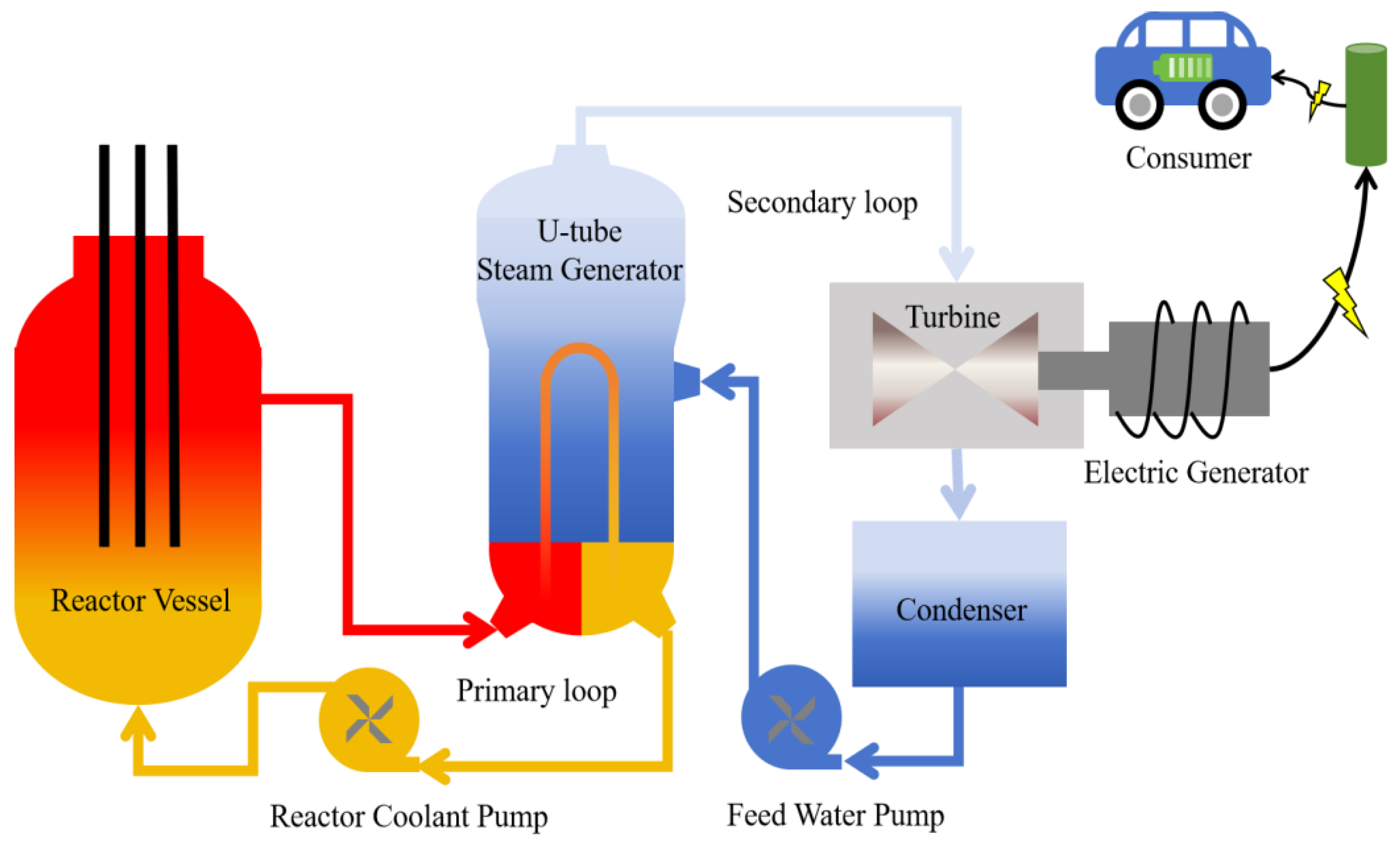Additionally, during reactor shutdown or certain accident conditions, it removes decay heat from the reactor core and prevents radioactive substances from leaking from the primary loop to the secondary loop [1,2]. The vertical U-tube natural circulation steam generator (UTSG) is the most commonly used form of steam generator in pressurized water reactor (PWR) nuclear power plants. The working principle of a PWR nuclear power plant using a UTSG is illustrated in Figure 1 [3,4].

To conduct efficiency assessments and optimize operations, the UTSG has been extensively studied, particularly in the areas of modeling and simulation. Various modeling approaches have been proposed for the UTSG, tailored to specific conditions. Xianping et al. proposed a transient lumped-parameter nonlinear dynamic model for the UTSG, which can be used for the development of steam discharge and bypass control systems as well as for coupling calculations with the primary loop system as a module [5]. By inputting the structural and operational parameters of the UTSG, the model can calculate parameters such as secondary side pressure, water level, and primary side outlet temperature. Sung et al. analyzed a steam generator tube rupture accident caused by a severe accident using a severe accident analysis program [6]. The steady-state calculation results of the analyzed object include parameters such as primary side pressure, temperature, flow rate, and secondary side pressure. Tenglong, ZengGuang, and Vivaldi each proposed three-dimensional analysis methods for the secondary side flow field of the steam generator, which are coupled with the primary side. These methods are used to determine the distribution of local flow velocity, void fraction, and temperature parameters on the secondary side of the steam generator [7,8,9].

In recent years, machine learning algorithms have been widely applied in the design and optimization of heat exchanger models. Shaopeng et al. developed a deep learning reduced-order model (ROM) based on proper orthogonal decomposition (POD) and machine learning (ML) methods. This model captures the implicit nonlinear mapping relationship between computational fluid dynamic (CFD) inputs and feature coefficients, enabling rapid estimation of the void fraction and temperature field distribution on the secondary side of the steam generator [10]. Emad et al. used four supervised machine learning algorithms to predict the effects of air injection and transverse baffles on the thermohydraulic performance of shell and tube heat exchangers [11]. Huai et al. analyzed and optimized the influence of inlet and outlet distribution on vapor–liquid two-phase flow and heat transfer characteristics using a genetic-based backpropagation neural network [12]. Andac et al. employed a feedforward neural network to forecast the heat transfer coefficient, pressure drop, Nusselt number, and performance evaluation criteria for a shell and helically coiled tube heat exchanger [13]. Mohammed et al. proposed a random vector functional link network to predict the outlet temperatures of working fluids in a helical plate heat exchanger [14]. Zafer et al. employed decision tree classification to investigate the impact of delta wing vortex generator design features on the thermohydraulic performance of heat exchangers [15]. Mahyar et al. predicted heat transfer in heat exchangers for turbulent flow using random forest, K-Nearest Neighbors, and support vector regression techniques [16].

Although current studies have developed UTSG computational models and optimization methods, there is a gap regarding the computational degrees of freedom of the model. Specifically, existing models are limited to using certain parameters as inputs to calculate designated output parameters. As a critical interface between the primary and secondary loops, the UTSG involves numerous interacting parameters. Fixed-structure computational models have inherent limitations and are unable to meet the demands of different operating conditions encountered in UTSG design. For example, under different design conditions, the known input parameters and the desired output parameters of the model vary. To address this issue, this study proposes a machine learning-based method for building a high-degree-of-freedom UTSG thermal model. The most notable feature of this approach is its ability to flexibly interchange input and output parameters, allowing it to directly adapt to the interface requirements of various application scenarios. This work provides four contributions: (1) A thorough sensitivity analysis of model parameters is conducted to determine the optimal approach for generating training datasets. (2) A high-degree-of-freedom UTSG thermal model is proposed using a lightweight machine learning algorithm, allowing for flexible interchange of input and output parameters. This versatility enables engineers to tailor the model to specific design and operational needs without extensive reconfiguration. (3) The model’s performance is thoroughly evaluated, demonstrating its robustness and practical applicability. (4) A screening strategy based on multiple sub-models is developed to eliminate anomalous predictions.

This paper is structured as follows: First, the UTSG model and the physical simplification process are introduced. Next, model parameter sensitivity analysis is presented, and three parameter sampling methods are proposed to generate the training dataset for machine learning. Then, the lightweight machine learning algorithm is described. This is followed by a series of validations and optimizations of the proposed machine learning pipeline. Finally, the main findings of the paper are summarized in the concluding section.

2. Model Description

The UTSG is a critical component in nuclear reactors, serving as a heat exchanger. Its operating principle involves the flow of reactor coolant through the interior of U-shaped tubes within the primary loop, where it transfers heat to the water in the secondary loop surrounding the tubes. The water in the secondary loop absorbs this heat, undergoes a phase change to steam, and subsequently drives a turbine generator to produce electricity. The UTSG effectively isolates the primary and secondary loop fluids, thereby preventing radioactive contamination while efficiently converting the reactor’s thermal energy into mechanical and electrical energy.

For the thermal–hydraulic analysis of the UTSG, a simplified physical model has been established based on the following assumptions [4,5]:

(1) The fluids on both the primary and secondary sides are assumed to be in one-dimensional flow.

(2) The fluid density variation along the flow direction is considered only when converting between volumetric flow rate and mass flow rate; otherwise, the fluid density in the U-tubes is assumed to be its average density.

(3) The secondary side of the steam generator operates under saturated boiling conditions, and subcooled boiling is not considered.

(4) The saturated pressure on the secondary side is assumed to be uniform.

(5) The thermal conductivity of the heat transfer tubes is assumed to be constant.

(6) The flow outside the convective heat transfer regions on both the primary and secondary sides is considered to be adiabatic.

After the aforementioned simplification, the structure of UTSG is shown in Figure 2. The corresponding simplified thermal model is described by the following equations, and the physical properties of water and steam are obtained through IAPWS-IF97.

Part I: Primary Side Model

$$\begin{array}{l}Q=w_p\left(i_{in,p}-i_{out,p}\right)\\ i_{in,p}=f\left(P_p,t_{in,p}\right)\\ i_{out,p}=f\left(P_p,t_{out,p}\right)\\ {\displaystyle \frac{\left(t_{in,p}+t_{out,p}\right)}{2}}=t_{ave,p}\end{array}$$

(1)

Here, Q is the thermal power, w_p is the mass flow rate of the primary side fluid, and P_p is the operating pressure of the primary side fluid. i_in,p and i_out,p are the enthalpies at the inlet and outlet of the primary side fluid, respectively. t_in,p, t_out,p, and t_ave,p are the inlet, outlet, and average temperatures of the primary side fluid, respectively.

$$\begin{array}{c}{w}_p=V_p\cdot {\rho }_{out,p}\\ {\rho }_{out,p}=f\left(P_p,t_{out,p}\right)\end{array}$$

(2)

Here, V_p is the volumetric flow rate of the primary side fluid, and ${\rho }_{out,p}$ is the density of the primary side fluid at the outlet.

Part II: Secondary Side Model

$$\begin{array}{c}{w}_f=w_s={\displaystyle \frac{Q}{i_s-i_f}}\\ t_s=f\left(p_s\right)\\ i_s=f\left(p_s\right)\\ i_f=f\left(P_s,t_f\right)\end{array}$$

(3)

Here, i_f and i_s are the enthalpies of the feedwater and steam, respectively. w_f and w_s are the flow rates of the feedwater and steam, respectively. p_s is the saturation pressure on the secondary side. t_s and t_f are the saturation temperature on the secondary side and the feedwater temperature, respectively.

Part III: Primary and Secondary Side Heat Transfer Model

$$\begin{array}{l}{v}_p={\displaystyle \frac{W_p}{{\rho }_{ave,p}\cdot N\cdot \frac{\pi }{4}\cdot {d_i}^2}}\\ d_i=d_o-2\delta \end{array}$$

(4)

Here, v_p is the flow velocity of the primary side fluid inside the heat transfer tubes. d_i and d_o are the inner and outer diameters of the heat transfer tubes, respectively. δ is the wall thickness of the heat transfer tubes, and N is the number of heat transfer tubes.

$$\begin{array}{l}{\alpha }_p=0.023\cdot {\mathrm{Re}}^{0.8}{\mathrm{Pr}}^{0.4}{\displaystyle \frac{{\lambda }_{ave,\rho }}{d_i}}\\ \mathrm{Re}={\displaystyle \frac{{\rho }_{ave,p}\cdot d_i\cdot v_p}{{\mu }_{ave,p}}}\\ {\rho }_{ave,p}=f\left(P_p,t_{ave,p}\right)\\ {\mu }_{ave,p}=f\left(P_p,t_{ave,p}\right)\\ \mathrm{Pr}=f\left(P_p,t_{ave,p}\right)\\ {\lambda }_{ave,p}=f\left(P_p,t_{ave,p}\right)\end{array}$$

(5)

Here, ${\alpha }_p$ is the convective heat transfer coefficient of the primary side fluid [7], ${\lambda }_{ave,\rho }$ is the average thermal conductivity of the primary side fluid, and R_e and P_r are the Reynolds number and Prandtl number, respectively. ${\rho }_{ave,p}$ is the average density of the primary side fluid, and ${\mu }_{ave,p}$ is the average viscosity of the primary side fluid.

$$\begin{array}{l}K={\displaystyle \frac{1}{\frac{1}{{\alpha }_p}\cdot \frac{d_o}{d_i}+\frac{1}{{\alpha }_s}+R_w+R_F}}\\ {\alpha }_s=57.59e^{\left({\displaystyle \frac{P_s}{15.5}}\right)}{\left(t_{ave,p}-t_s\right)}^3\\ R_w={\displaystyle \frac{d_o}{2\cdot {\lambda }_{tube}}}\ln \left({\displaystyle \frac{d_o}{d_i}}\right)\end{array}$$

(6)

Here, K is the heat transfer coefficient of the UTSG, ${\alpha }_s$ is the convective heat transfer coefficient on the secondary side [7], R_w is the thermal resistance of the heat transfer tube wall, and ${\lambda }_{tube}$ is the thermal conductivity of the heat transfer tube material.

$$\begin{array}{l}Q=KA\Delta t\\ \Delta t={\displaystyle \frac{t_{in,p}-t_{out,p}}{\ln \left(\frac{t_{in,p}-t_s}{t_{out,p}-t_s}\right)}}\end{array}$$

(7)

Here, A is the heat transfer area, and $\Delta t$ is the logarithmic mean temperature difference.

From the above equations, it is evident that the thermal calculation of UTSGs involves 16 known and unknown quantities, encompassing operating parameters, structural parameters, and other variables. The primary side parameters include [Q, P_p, V_p, t_ave,p, t_in,p, t_out,p]. The secondary side parameters include [p_s, w_f, w_s, t_f]. The structural parameters include [d_o, δ, A, N]. Additionally, [λ_tube, R_F] represent the physical property of the heat transfer tube material and the fouling thermal resistance, respectively, as adopted by the designer based on experience. The remaining parameters are intermediate quantities, including fluid physical property, flow velocity, heat transfer coefficients, and the logarithmic mean temperature difference.

To verify the calculation accuracy of the simplified UTSG thermal model, this section compares the results of the simplified model with those of the non-simplified model used in reference [4] under the same set of parameters, as shown in

Table 1. A comparison of the calculation results between the simplified UTSG model and the reference model.

Model given input
Variable	Unit	Value
Q	[W]	7.33 × 108
Pp	[MPa]	15.51
tin,p	[°C]	316.7
Vp	[m3/h]	20,404.7
do	[m]	22.23
δ	[m]	1.27
N	[-]	3260
RF	[m2 · °C/W]	5.28 × 10−5
Rw	[m2 · °C/W]	8.15 × 10−5
A	[m2]	4127.7
tf	[°C]	223.9
Model calculation output
Variable	Unit	Simplified model	Reference
tout,p	[°C]	285.7	285.7
ps	[MPa]	5.44	5.41
ws	[kg/s]	401.2	402.7
wf	[kg/s]	401.2	402.7

. The results indicate that the calculation results of the two models are very close.

3. Framework of the Proposed High-Degree-of-Freedom UTSG Thermal Model

Typically, the design of UTSGs relies on specialized design software. This type of software generally offers one or several fixed-structure input–output model structures. Specifically, the software built based on Equations (1)–(7) in Section 2 uses eight parameters [Q, V_p, t_in,p, d_o, δ, A, N, t_f] as software input parameters, and three model parameters [t_out,p, p_s, w_s] are the software output parameters. For practical applications, these fixed-structure models pose a problem due to limited design flexibility, as the provided input parameters can vary. For example, if the eight input parameters are now [Q, A, t_in,p, d_o, δ, t_out,p, p_s, w_s], the UTSG model in its current form (modeled by Equations (1)–(7)) cannot provide the calculation results for the rest of the three parameters [V_p, N, t_f]. To address this issue, there are typically two solutions. The first approach is to establish a new model structure for the new unknown and known variables and redesign the calculation software. The second approach is to find the required solutions based on extensive trial calculations and regression techniques. However, both methods are time-consuming and require expert knowledge.

Enhancing the flexibility of the UTSG thermal model is essential for improving its computational efficiency in practical applications. To achieve this, we propose a machine learning-based high-degree-of-freedom UTSG calculation model. The overall process framework of the proposed algorithm is illustrated in Figure 2. Firstly, feature engineering techniques are used to reduce feature dimensions and improve the quality of the generated training dataset. To achieve this, we analyze the original equation structure of UTSGs and, with expert knowledge, eliminate parameters considered constant in practical applications, thereby reducing the complexity of model training. Subsequently, we use a local sensitivity analysis method to assess the sensitivity of various UTSG model parameters. Based on the sensitivity analysis results, we design different parameter sampling methods to generate the training set for the machine learning algorithm. After generating the training dataset, the UTSG mathematic model that consists of a set of system equations is no longer needed. Finally, we develop a lightweight feedforward neural network to construct a machine learning algorithm that allows for a flexible selection of known input parameters and unknown output parameters in the UTSG model. The input of the proposed machine learning model is eight randomly chosen parameters (e.g., [Q, A, t_in,p, d_o, δ, t_out,p, p_s, w_s]), and the output of the proposed ANN model is the corresponding three remaining parameters [V_p, N, t_f]. This proposed framework enables arbitrary selection of the input and output parameters of the UTSG model, significantly enhancing its computational flexibility.

4. Parameter Sensitivity Analysis

The UTSG thermal model studied in this work is described by Equations (1)–(7). This model includes multiple physical parameters, which need to be obtained from highly nonlinear physical property tables (i.e., f(.)). To reduce the computational complexity of this complex nonlinear system, this paper employs expert knowledge and sensitivity analysis to perform data dimensionality reduction on the parameters. In pressurized water reactor nuclear power plants, P_p is typically 15.51 MPa, and R_F is a constant value provided by the designer. The heat transfer tubes of the UTSG in third-generation nuclear power plants are mainly made of nickel-based alloys, resulting in a small variation range for λ_tube. Due to mass conservation, w_f and w_s are equal, so this study only retains w_s. Based on the above analysis, in this study, [P_p, R_F, λ_tube] are set as constant values in the UTSG model, leaving the remaining model parameters as [Q, V_p, t_in,p, t_out,p, d_o, δ, A, N, p_s, w_s, t_f].

Next, this section evaluates the sensitivity of the UTSG thermal model parameters based on local sensitivity analysis. Parameters with high sensitivity have a significant impact on the model’s output, whereas changes in low-sensitivity parameters have a negligible effect. Therefore, based on the sensitivity analysis results, we can design parameter sampling methods more effectively, thereby generating machine learning training datasets more efficiently and improving the prediction accuracy of the machine learning algorithm.

After dimensionality reduction of the model parameters based on expert knowledge, the input parameters of the UTSG thermal model are M = [Q, V_p, t_in,p, d_o, δ, A, N, t_f], and the corresponding model outputs are Y = [t_out,p, p_s, w_s]. Let the nonlinear mapping function between the inputs and outputs be f, then the three outputs of the model can be described as follows:

$$Y=\left[\begin{array}{c}{t}_{outp}\\ p_s\\ w_s\end{array}\right]=\left[\begin{array}{c}{f}_1\left(M\right)\\ f_2\left(M\right)\\ f_3\left(M\right)\end{array}\right]$$

(8)

The sensitivity matrix corresponding to the above model can be written as follows:

$$S^M={\left[\begin{array}{cccc}{\displaystyle \frac{\partial f_1\left(M\right)}{\partial Q}}{\displaystyle \frac{Q_{norm}}{f_1\left(M_{norm}\right)}},& {\displaystyle \frac{\partial f_1\left(M\right)}{\partial V_p}}{\displaystyle \frac{{V_p}^{nom}}{f_1\left(M_{norm}\right)}},& \cdots & {\displaystyle \frac{\partial f_1\left(M\right)}{\partial t_f}}{\displaystyle \frac{t_{f,norm}}{f_1\left(M_{norm}\right)}}\\ {\displaystyle \frac{\partial f_2\left(M\right)}{\partial Q}}{\displaystyle \frac{Q_{norm}}{f_2\left(M_{norm}\right)}},& {\displaystyle \frac{\partial f_2\left(M\right)}{\partial V_p}}{\displaystyle \frac{{V_p}^{nom}}{f_2\left(M_{norm}\right)}},& \cdots & {\displaystyle \frac{\partial f_2\left(M\right)}{\partial t_f}}{\displaystyle \frac{t_{f,norm}}{f_2\left(M_{norm}\right)}}\\ {\displaystyle \frac{\partial f_3\left(M\right)}{\partial Q}}{\displaystyle \frac{Q_{norm}}{f_3\left(M_{norm}\right)}},& {\displaystyle \frac{\partial f_3\left(M\right)}{\partial V_p}}{\displaystyle \frac{{V_p}^{nom}}{f_3\left(M_{norm}\right)}},& \cdots & {\displaystyle \frac{\partial f_3\left(M\right)}{\partial t_f}}{\displaystyle \frac{t_{f,norm}}{f_3\left(M_{norm}\right)}}\end{array}\right]}_{3\times 11}$$

(9)

where the subscript norm represents the nominal values of the parameters.

In Equation (9), the sum of each column represents the sensitivity of the corresponding model parameter. For example, the sensitivity of the model parameter Q is as follows:

$$S_Q={\displaystyle \frac{\partial f_1\left(M\right)}{\partial Q}}{\displaystyle \frac{Q_{norm}}{f_1\left(M_{norm}\right)}}+{\displaystyle \frac{\partial f_2\left(M\right)}{\partial Q}}{\displaystyle \frac{Q_{norm}}{f_2\left(M_{norm}\right)}}+{\displaystyle \frac{\partial f_3\left(M\right)}{\partial Q}}{\displaystyle \frac{Q_{norm}}{f_3\left(M_{norm}\right)}}$$

(10)

Due to the strong nonlinearity of the UTSG thermal model, the gradient terms in Equation (10) are calculated using a finite difference scheme. Given a perturbation value Δ applied to parameter Q, using the first-order forward difference scheme, Equation (10) can be written as follows:

$$S_Q={\displaystyle \frac{f_1\left(M+\Delta \right)-f_1\left(M\right)}{\Delta }}{\displaystyle \frac{Q_{norm}}{f_1\left(M_{norm}\right)}}+{\displaystyle \frac{f_2\left(M+\Delta \right)-f_2\left(M\right)}{\Delta }}{\displaystyle \frac{Q_{norm}}{f_2\left(M_{norm}\right)}}+{\displaystyle \frac{f_3\left(M+\Delta \right)-f_3\left(M\right)}{\Delta }}{\displaystyle \frac{Q_{norm}}{f_3\left(M_{norm}\right)}}$$

(11)

When performing the local sensitivity analysis, it is necessary to determine the magnitude of the baseline values M_norm. To eliminate the impact of different baseline value selections on the sensitivity analysis results, this paper conducts sensitivity analysis using the nominal values, upper limit values, and lower limit values of each parameter. The results are shown in Figure 3.

As shown in Figure 3, the selection of baseline values affects the absolute values of the UTSG thermal model parameter sensitivities to some extent. However, the consistency of the relative sensitivity ranking of the parameters remains very high. Specifically, the sensitivity of the model parameter t_in,p is significantly higher than that of other parameters, while the sensitivity of N is significantly lower than that of other parameters. Based on the results of the sensitivity analysis, this work will adopt three different strategies for generating machine learning training datasets in the subsequent research:

Method 1: Allocate more sampling points to the most sensitive model parameters and fewer to the least sensitive ones. The remaining parameters will receive an equal number of sampling points.

Method 2: Set an equal number of sampling points for all model parameters, i.e., uniform sampling.

Method 3: In contrast to the approach in Method 1, allocate the most sampling points to the least sensitive parameters and the fewest sampling points to the most sensitive parameters. The remaining parameters will receive an equal number of sampling points.

The impact of the above three sampling methods on the accuracy of the proposed machine learning algorithm will be discussed in the subsequent sections.

5. A Lightweight Machine Learning-Based Method for Predicting UTSG Model Outputs

5.1. Construction of the Machine Learning Training Set

The quality of the training dataset significantly impacts the performance of a machine learning algorithm. To ensure that the developed machine learning algorithm possesses high prediction accuracy and generalization ability, this study constructs a comprehensive training dataset by performing a parametric scan of the model parameters, resulting in a diverse array of parameter combinations. As shown in

Table 2. Parameter range settings for generating data samples.

Parameters	Ref	Lower Bound/Ref, %	Upper Bound/Ref, %	Sampling Number
				M1 1	M2 1	M3 1
Q	7.33 × 108	90%	240%	3	3	3
Pp	15.51	-	-	1	1	1
$t_{in,p}$	316.7	92%	102%	4	3	2
Vp	20,404.7	95%	170%	3	3	3
do	22.23	75%	105%	3	3	3
δ	1.27	75%	105%	3	3	3
N	3260	95%	310%	2	3	4
$R_F$	5.28 × 10−5	-	-	1	1	1
${\lambda }_{tube}$	18.8	-	-	1	1	1
A	4127.68	95%	230%	3	3	3
$t_f$	223.9	95%	105%	3	3	3
Number of Valid Samples				320	320	320

¹ M represents different sampling methods as discussed in Section 4.

, 320 valid samples were generated by employing mean value sampling between the upper and lower limits of each parameter. Table 2 includes three different sampling methods (columns 5–7), corresponding to sampling methods 1, 2, and 3 described in Section 4.

It is worth noting that to obtain the 320 valid samples, large-scale data generation was necessary during the sample generation process. This is because the parameter combinations generated in Table 2 are random, and for some parameter combinations, the UTSG thermal model calculations may not converge, requiring those results to be excluded. The relationship between the original number of samples and the number of valid samples for different sampling methods is shown in Figure 4.

After generating the valid samples, the next step is to construct the training dataset for the machine learning algorithm. The core of a machine learning algorithm is to establish the complex mapping relationship between inputs and outputs. Therefore, constructing the input–output structure of the training dataset is a crucial step in training the machine learning model. By analyzing Equations (1)–(7), the parameter input–output relationship of the UTSG model can be written as follows:

$$\stackrel{Input}{\left[\begin{array}{cccc}{Q}_1& V_{p,1}& t_{in,p,1}& V_{o,1}\\ Q_2& V_{p,2}& t_{in,p,2}& d_{o,2}\\ ⋮& ⋮& ⋮& ⋮\\ Q_L& V_{p,L}& t_{in,p,L}& d_{o,\mathrm{L}}\end{array}\begin{array}{c}{\delta }_1\\ {\delta }_2\\ ⋮\\ {\delta }_L\end{array}\begin{array}{c}{A}_1\\ A_2\\ ⋮\\ A_L\end{array}\begin{array}{c}{N}_1\\ N_2\\ ⋮\\ N_L\end{array}\begin{array}{c}{t}_{f,1}\\ t_{f,2}\\ ⋮\\ t_{f,\mathrm{L}}\end{array}\right]}\to \stackrel{Output}{\left[\begin{array}{c}{t}_{out,p,1}\\ t_{out,p,2}\\ ⋮\\ t_{out,p,L}\end{array}\begin{array}{c}{p}_{s,1}\\ p_{s,2}\\ ⋮\\ p_{s,L}\end{array}\begin{array}{c}{w}_{s,1}\\ w_{s,2}\\ ⋮\\ w_{s,L}\end{array}\right]}$$

(12)

where the subscript [1,2,…L] represents the values of the parameters under different sampling instances.

After training with the dataset shown in Equation (12), the machine learning algorithm can calculate the corresponding output values [t_out,p, p_s, w_s] when the parameters [Q, V_p, t_in,p, d_o, δ, A, N, t_f] are used as inputs. As previously mentioned, the focus of this study is to freely choose the known and unknown quantities of the UTSG calculation model, thereby enhancing the computational flexibility of the UTSG model. For example, parameters [Q, t_in,p, t_out,p, d_o, δ, N, p_s, w_s] can be used as inputs to solve for variables [V_p, A, t_f].

To achieve a flexible selection of input parameters, this study innovatively proposes the training dataset structure design strategy illustrated in Figure 5.

As shown in Figure 5, in the training data structure design strategy, the input data dimension is equal to the sum of the model input and output parameters (i.e., 8 + 3 = 11). For a specific input–output parameter mapping relationship, the corresponding output parameters in the input data matrix are set to zero, thereby achieving a flexible selection of input parameters and covering all possible parameter combinations. Specifically, the proposed prediction model can arbitrarily select 8 out of 11 variables as inputs and predict the remaining 3 variables. After constructing the training dataset as shown in Figure 5, the training matrix will contain $C_{11}^3=165$ different parameter combinations for the same set of model parameters. Therefore, the 320 parameter combinations generated in Table 2 will expand to a training dataset with dimensions of 52,800 × 11 after constructing the training dataset as shown in Figure 5, significantly increasing the dataset’s dimensions. It is important to note that due to the structural characteristics of the UTSG thermal model, there are 76 parameter combinations that render the original system of equations (i.e., Equations (1)–(7)) unsolvable (i.e., the system does not have a unique solution). Therefore, these 76 parameter combinations need to be excluded during the training data generation process, as shown in Figure 5c. Ultimately, the 320 parameter combinations generated in Table 2 will expand to a training dataset with dimensions of 28,480 × 11, which will be used for subsequent machine learning algorithm training and testing.

As can be seen from Figure 5, we considered all the possible combinations of the input parameters for the UTSG model. For example, the first line in Figure 5b means [Q, V_p, t_in,p, d_o, δ, A, N, t_f] are the input parameters, and [t_out,p, p_s, w_s] are the output parameters, while the last line in Figure 5b means [t_out,p, p_s, w_s, d_o, δ, A, N, t_f] are the input parameters, and [Q, V_p, t_in,p] are the output parameters.

5.2. Feedforward Neural Network Based on Backpropagation Learning Strategy

In recent years, machine learning algorithms have been widely applied in fields such as finance, energy, and numerical computation [17]. Given sufficient computational power and data, deep learning frameworks can exhibit excellent performance. However, the objective of this study is to enhance the flexibility of practical engineering design software using machine learning. Such engineering design software typically runs on standard computers with limited computational power. Therefore, this paper adopts a lightweight feedforward neural network to construct the machine learning algorithm framework.

A feedforward neural network is one of the simplest neural network structures. Due to its lower computational complexity, feedforward neural networks have become the most widely used and rapidly developing neural network structures. In this network structure, information flows unidirectionally from the input layer to the hidden layer and finally to the output layer. Each neuron in a feedforward neural network is only connected to the neurons in the previous layer, passing the received output from the previous layer to the next layer, with no feedback loops between the layers. To learn the weight values of the parameters in the feedforward neural network, this paper employs the backpropagation (BP) algorithm. The overall structure of the BP-FNN neural network is shown in Figure 6, which includes the input layer, hidden layer, and output layer.

For the single hidden layer BP-FNN neural network shown in Figure 6, let the input layer have n nodes, the hidden layer have q nodes, and the output layer have m nodes. The weight matrix between the input layer and the hidden layer is V, and the weight matrix between the hidden layer and the output layer is W. Let the input layer variables be x. The outputs of the hidden layer and the output layer can be expressed as follows:

$$Z_k=f_1\left({\displaystyle \sum _{i=1}^n{V}_{ki}{X}_i}\right),k=1\cdots q$$

(13)

$${Y_j}^{\prime }=f_2\left({\displaystyle \sum _{k=1}^q{W}_{jk}{Z}_k}\right),j=1\cdots m$$

(14)

where, f₁ and f₂ are the activation function for the hidden layer and output layer, respectively, and are typically chosen as the sigmoid function in the BP-FNN. Z_k is the output of the k-th hidden unit, and Y’_j is the output of the j-th output unit.

Assuming the training data consist of p samples, the error function for each sample is given by

$$E_p={\displaystyle \frac{1}{2}}{{\displaystyle \sum _{j=1}^m\left(y_{jp}-{y^{\prime }}_{jp}\right)}}^2$$

(15)

Finally, the weights W and V in the BP-FNN are updated using the gradient descent method. The updated formulas are as follows:

$$\Delta W_{jk}=-\eta {\displaystyle \frac{\partial E_p}{\partial W_{jk}}},\Delta V_{ki}=-\eta {\displaystyle \frac{\partial E_p}{\partial V_{ki}}}$$

(16)

where η is the learning rate.

In the constructed BP-ANN, the activation function is the hyperbolic tangent sigmoid. The learning rate is set at 0.01, and a dropout rate of 0.2 is applied to prevent overfitting.

5.3. Model Prediction Accuracy

5.3.1. BP-ANN Prediction Error Distribution

As described in Section 5, 320 training samples were generated. Subsequently, as shown in Figure 5, after constructing the training dataset and excluding parameter combinations that make the system of equations non-closed, a training dataset with dimensions of 28,480 × 11 was generated. First, 80% of the training data (22,784 samples) were used to train the BP-ANN model, and the remaining 20% of the data (5696 samples) were used for testing. In the proposed machine learning pipeline, the BP-ANN has three units in the output layer, each corresponding to one model output. Consequently, the BP-ANN selects eight random parameters as inputs and predicts the remaining three parameters.

To evaluate the prediction accuracy, the mean absolute relative error (MARE) is utilized in this study. The MARE is calculated as follows:

$$\mathrm{MARE}={\displaystyle \frac{1}{M}}{\displaystyle {\sum }_{i=1}^M\left(\frac{\left|y_i-y_{i,p}\right|}{y_i}\right)}$$

(17)

where M is the number of data points. y_i is the true value and y_i,p is the predicted value for the i-th data point.

Artificial neural networks generate different results with each training session primarily due to random weight initialization, the stochastic gradient descent optimization strategy, and regularization techniques such as dropout. To comprehensively verify model accuracy, the BP-ANN was run 10 times, and the prediction results for all 11 UTSG model parameters are reported, as shown in Figure 7. From Figure 7, the prediction errors for all the input parameter combinations are shown. According to the input–output structure of the proposed BP-ANN, eight randomly selected parameters are used as input features, and the remaining three parameters are BP-ANN prediction outputs. During the testing of the 5896 samples, three different categories of parameters will be selected as prediction outputs each time. After testing all 5896 samples, all 11 UTSG model parameters will appear in the output at least once during one of the tests. In Figure 7, the error distributions for each model parameter are presented using histograms. The error distributions for the best case (green) and worst case (red) are displayed, with the average performance of the BP-ANN shown in blue. Additionally, each histogram plot includes mean values (gray dashed line) and maximum values (black dashed line) for prediction errors. Figure 7 demonstrates that the proposed BP-ANN-based UTSG model can accurately predict each of the 11 UTSG model parameters.

To generate the results for Figure 7, the number of neurons was set to 200, and the training dataset was generated using sampling method 1 (see Section 4). To study the effects of neuron numbers and sampling methods, we compared the BP-ANN performance with different neuron numbers ranging from 50 to 200. For each neuron number, sampling methods 1, 2, and 3 (see Section 4) were used to generate the training datasets. The comparative results are shown in Figure 8. For each training sample, the input and output parameters are different. Therefore, in Figure 8, we focus solely on the prediction accuracy of each BP-ANN output unit (i.e., BP-ANN outputs 1–3). From Figure 8, two key findings emerge. First, the accuracy of the proposed BP-ANN model increases with the number of neurons. However, increasing the number of neurons also raises the model’s complexity, presenting a trade-off between accuracy and efficiency. Second, the training dataset generated by sampling method 1 yields the best accuracy. According to Section 4, sampling method 1 allocates more sampling points to the most sensitive model parameters and fewer to the least sensitive ones. This conclusion holds across all results, indicating that analyzing parameter sensitivity helps improve the prediction accuracy of the proposed machine learning framework.

Generally, the split between training and testing datasets (defined as the training data ratio) significantly impacts the accuracy of machine learning algorithms. To explore this effect on model accuracy, we used datasets generated by sampling method 1 and varied the training data ratios from 40% to 80%. The prediction accuracy of the proposed BP-ANN model under different neuron numbers is shown in Figure 9. It is evident that increasing the training data ratio leads to improved prediction accuracy.

When the number of neurons is set to 200, the prediction error for any of the three outputs remains below 3.2%, even when using only 40% of the data for training.

Additionally, due to the unique structure of the UTSG model, not all parameter input combinations yield a unique solution. In other words, different values for the same parameter set can produce the same output from the model. This multi-solution problem reduces the prediction accuracy of the machine learning method. By identifying these special cases as anomalies for the UTSG model, we can exclude 76 samples from the training dataset to improve overall accuracy. In this subsection, we investigate the effect of these abnormal cases on model accuracy, as shown in

Table 3. Impact of different constraint conditions on prediction accuracy.

MARE [%]	All Constraints	First 50% Constraints	Later 50% Constraints	No Constraints
Output 1	2.44	3.52	3.23	3.82
Output 2	2.80	3.93	4.01	4.61
Output 3	1.85	2.59	2.63	3.01

. In Table 3, “All constraints” indicates that all 76 abnormal samples are excluded from the training dataset. “First 50% constraints” removes the first 38 abnormal samples, while “Later 50% constraints” removes the last 38 abnormal samples. Additionally, we present the prediction accuracy when all these abnormal samples are included in the training dataset (i.e., “No constraints”).

5.3.2. Outlier Screening Strategy Based on Multiple Sub-Models

As described in Section 5.3.1, the proposed BP-FNN framework can accurately predict any parameter of the UTSG thermal calculation model. To further enhance the prediction accuracy of this framework, this section proposes an outlier screening strategy based on the mean of multiple sub-models, as shown in Figure 10.

Based on the training dataset, this section trained 10 different BP-FNN sub-models (i.e., BP-FNN #1 to BP-FNN #10), each having the same neural network structure. Upon completing training and making predictions, each sub-model predicted three output values (each corresponding to one output unit and as shown in Equation (18)). As illustrated in Figure 10, a training set with dimensions of 28,480 × 11 was generated for this study, with 80% of the data used for training and the remaining 20% used for validation. Consequently, the multi-sub-model structure depicted in Figure 10 generates 10 prediction matrices, each with dimensions of 5696 × 3.

$$\left[\begin{array}{c}Output1\\ Output2\\ Output3\end{array}\right]={\left[\begin{array}{ccc}\stackrel{\mathrm{BP}-\mathrm{FNN}\#1}{\overbrace{\begin{array}{ccc}output{1}_{1,1}& \cdots & output{1}_{1,5696}\\ output{2}_{1,1}& \cdots & output{2}_{1,5696}\\ output{3}_{1,1}& \cdots & output{3}_{1,5696}\end{array}}}& \cdots & \stackrel{\mathrm{BP}-\mathrm{FNN}\#10}{\overbrace{\begin{array}{ccc}output{1}_{10,1}& \cdots & output{1}_{1,5696}\\ output{2}_{10,1}& \cdots & output{2}_{1,5696}\\ output{3}_{10,1}& \cdots & output{3}_{1,5696}\end{array}}}\end{array}\right]}_{3\times 56960}$$

(18)

For the three outputs (i.e., Output 1 to 3), each output has 5696 × 10 prediction results. Based on the prediction values generated by the 10 sub-models, this section designed the following outlier screening strategy:

(1) Calculate the mean of each row in the matrix as shown in Equation (18), denoted as [output1_avg, output2_avg, output3_avg].

(2) Iterate through each row of the matrix shown in Equation (18) and calculate the mean value outputi_avg of each row. Then, eliminate the outlier output_i with the largest deviation from the mean.

(3) Calculate the mean of each row in the matrix as shown in Equation (18), and use this mean as the final predicted value.

Through this outlier screening strategy, when the predicted value of a sub-model is excessively high or low, it can be effectively corrected using the mean of the predicted values from the other neural network sub-models. This approach further enhances the prediction accuracy of the proposed BP-FNN-based UTSG model.

Table 4. Comparison of prediction accuracy for different BP-FNN frameworks.

Number of Neurons	Training Data Ratio	Single BP-FNN MARE [%]			Multi-Sub-Model BP-FNN MARE [%]
		Output 1	Output 2	Output 3	Output 1	Output 2	Output 3
50	80%	4.98	5.89	4.64	3.49	4.90	4.22
100		3.22	4.22	3.00	2.64	3.91	2.50
200		2.44	2.80	1.85	1.91	2.06	1.75
200	40%	2.75	3.15	2.12	2.44	2.59	1.82
	50%	2.64	3.14	2.04	2.41	2.51	1.75
	60%	2.55	2.85	1.93	2.21	2.48	1.52
	70%	2.46	2.82	1.91	1.85	2.30	1.36

compares the prediction accuracy between the single BP-FNN structure described in Section 5.3.1 and the multi-sub-model BP-FNN structure presented in this section. As shown in Table 4, the proposed outlier screening strategy results in a significant improvement in the model’s prediction accuracy under different numbers of neurons and various training data ratios, with the maximum improvement in prediction accuracy reaching up to 50%.

5.4. Comparison to Different Machine Learning Methods

To evaluate the performance of the proposed high-degree-of-freedom calculation method more comprehensively, we compared it with different methods in this section. To solve the multi-input (i.e., eight features) and multi-output (i.e., three prediction outputs) problem, we employed the Least Squares Support Vector Regression (LSSVR) and Bootstrap Aggregated Decision Trees (TreeBagger) algorithms for comparison.

Differing from the standard support vector regression method which typically involves solving a quadratic programming problem, LSSVR uses the least squares method to formulate the regression problem, resulting in a linear set of equations. By converting the optimization problem into solving a set of linear equations, LSSVR is more computationally efficient, especially for large datasets. More details about the LSSVR toolbox utilized in this section can be found in reference [18]. TreeBagger constructs multiple decision trees and combines their outputs to produce a more accurate and robust model compared to individual decision trees. To improve the stability and accuracy, the Bootstrap Aggregation (Bagging) method is used in TreeBagger [19]. In this section, three TreeBagger sub-models are constructed, each corresponding to a prediction output for the UTSG model.

For comparison, the BP-FNN model built in Section 5.2 is used as the benchmark. The same dataset is used to train the LSSVR and TreeBagger models, and their prediction results are compared. For a more comprehensive comparison, the following hyperparameter settings are considered:

(1) ANN-100: The BP-ANN using 100 neurons in its hidden layer is used.

(2) ANN-200: The BP-ANN using 100 neurons in its hidden layer is used.

(3) LSSVR-10: The regularization parameter gamma is set as 10. A larger gamma value results in a smoother model with fewer support vectors.

(4) LSSVR-1: The regularization parameter gamma is set as 1. A smaller gamma value allows for the model to include more support vectors for better fitting of the training data.

(5) TreeBagger-100: The number of decision trees in the forest is set to 100.

(6) TreeBagger-200: The number of decision trees in the forest is set to 200.

The performance of the above six machine learning models is compared, and the results are summarized in

Table 5. Predication accuracy of different machine learning models.

Number	Model Type	MARE [%]
1	ANN-100	3.48
2	ANN-200	2.36
3	LSSVR-1	5.11
4	LSSVR-10	3.45
5	TreeBagger-100	4.07
6	TreeBagger-200	2.89

. Two findings can be drawn from Table 5. First, the proposed UTSG high-degree-of-freedom calculation framework is broadly applicable to various machine learning algorithms. Second, the prediction performance of the various machine learning algorithms is similar, with BP-ANN exhibiting the highest accuracy.

6. Conclusions

The thermal calculation of steam generators is a critical analytical problem in practical applications. Traditional thermal calculation software, with its fixed input–output structures, lacks the adaptability to varying working conditions and application scenarios. This paper introduces a novel approach using the BP-ANN algorithm to develop a high-degree-of-freedom UTSG thermal model. The lightweight machine learning model employed requires minimal training data and has low computational complexity. The proposed UTSG model demonstrates high accuracy, with a maximum average calculation error of less than 2.1%.

A key feature of this method is its ability to freely interchange input and output parameters, allowing it to adapt to the varying requirements of different application scenarios. This flexibility significantly enhances the model’s robustness and practical applicability. This advancement opens new possibilities for optimizing UTSG performance under a wide range of operating conditions, providing a valuable tool for engineers and researchers. Moreover, the proposed method enables us to obtain the steady-state conditions of the UTSG more efficiently. Consequently, we can establish a baseline understanding of the heat transfer efficiency, pressure drops, and overall thermal–hydraulic behavior of the UTSG. This foundational knowledge is crucial for optimizing the design and operation of the UTSG, ensuring its reliable and efficient performance within a nuclear reactor system. Future work can further integrate this flexible modeling framework with other advanced machine learning techniques to enhance predictive capabilities and extend its application to more complex thermal systems. Additionally, the proposed method has only been validated on the U-tube steam generator. In the future, further verification is needed on other types of steam generator equipment, such as horizontal steam generators and helical coil steam generators.