
CFD Research on Natural Gas Sampling in a Horizontal Pipeline

Abstract
:1. Introduction
2. Mathematical Model
2.1. Governing Equations
2.2. Turbulence Model
3. Numerical Simulation
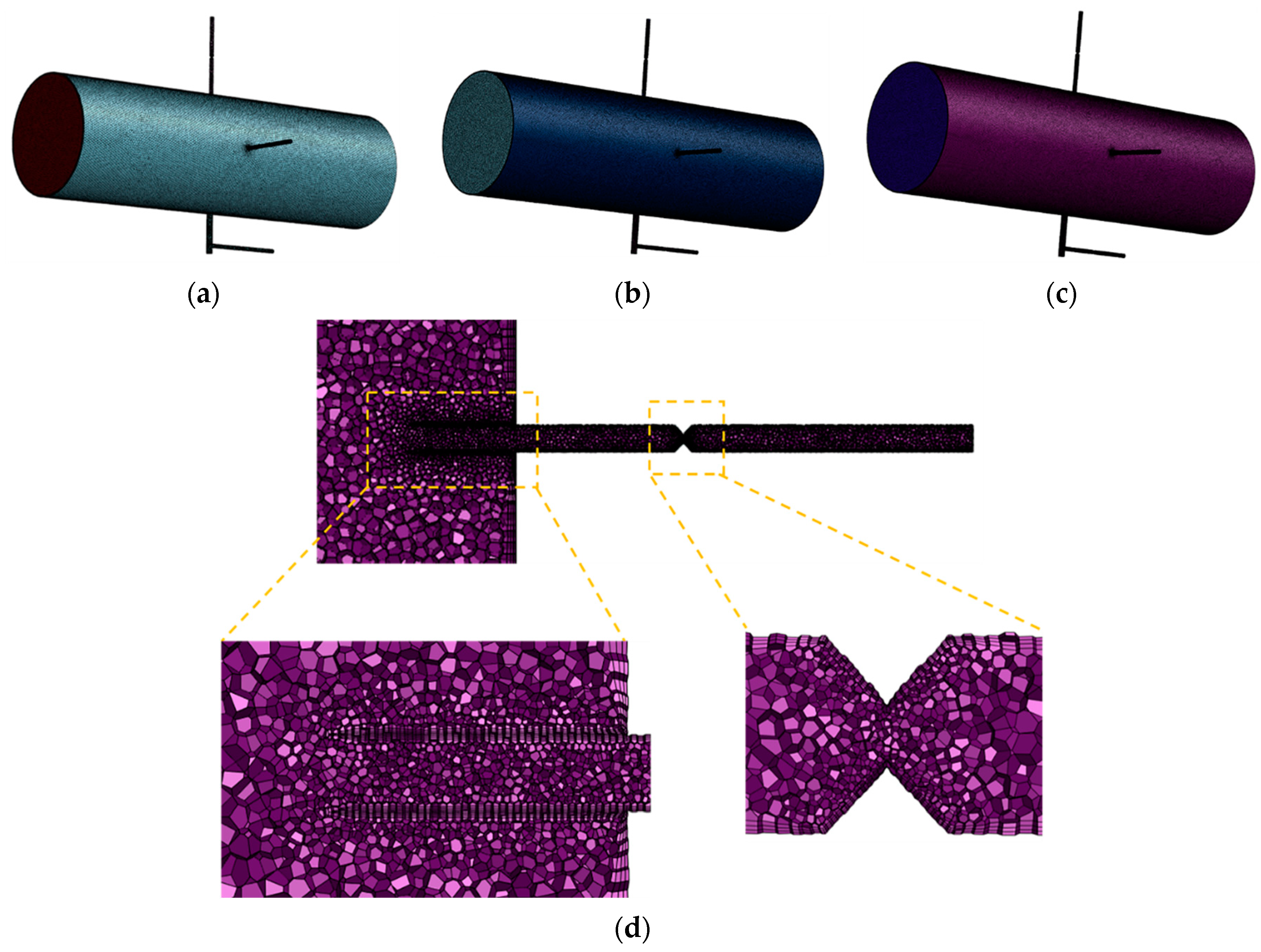
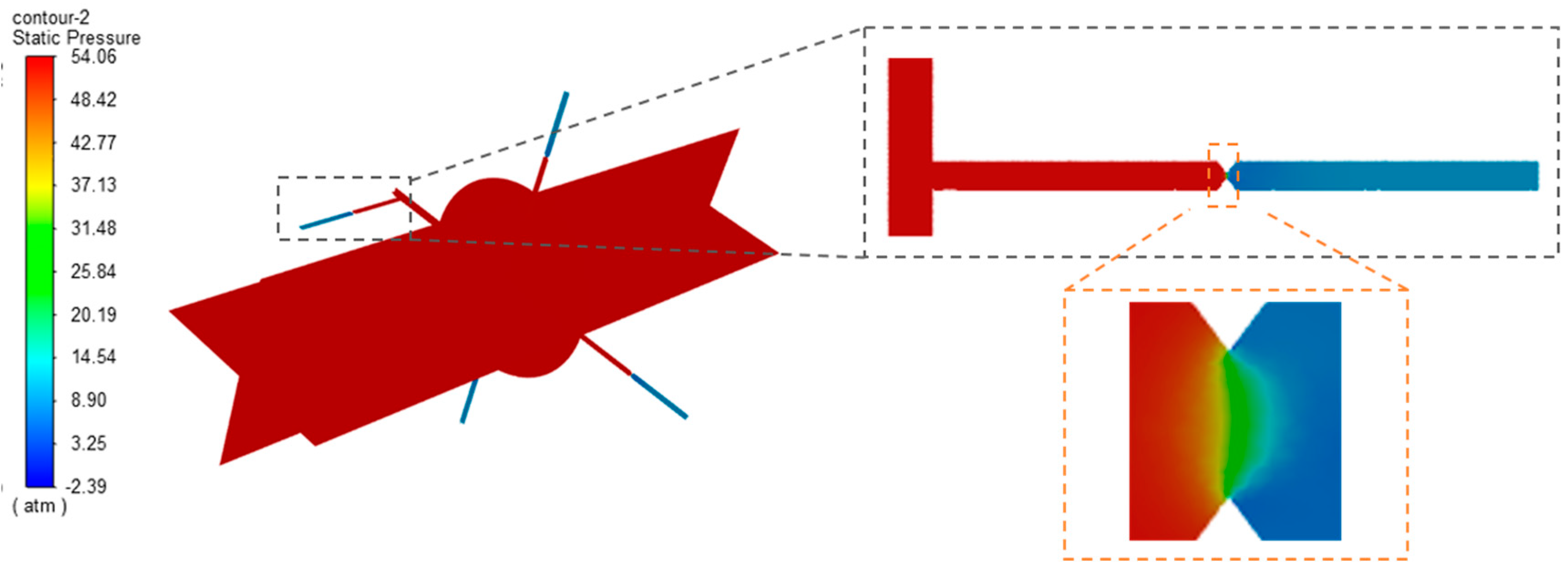
3.1. Geometrical Model
3.2. Numerical Setup
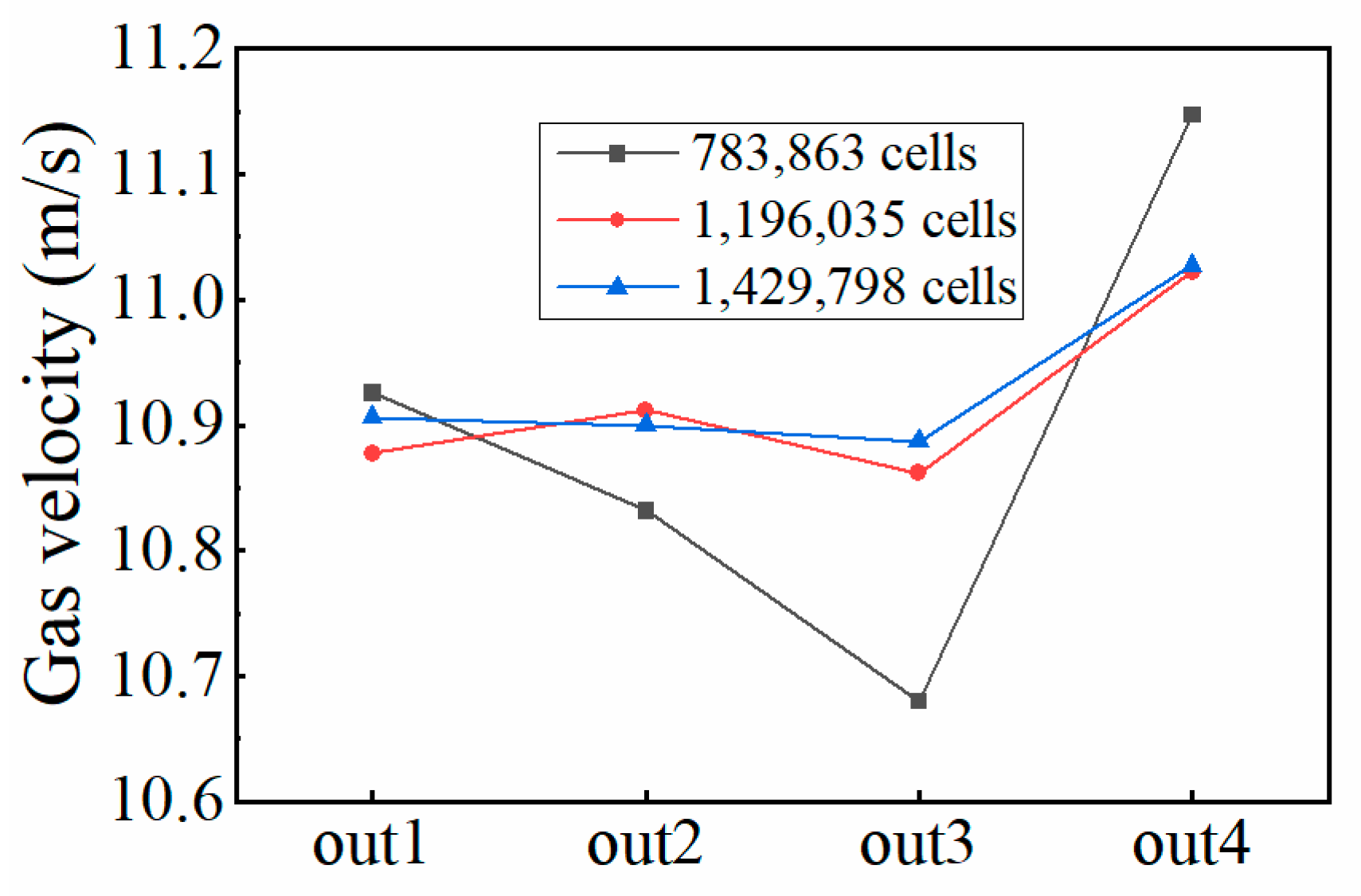
3.3. Grid Independency Study
4. Result and Discussion
4.1. Analysis of the Influence of Gravity
4.2. Influence of the Sampling Operating Conditions on Particle Parameters
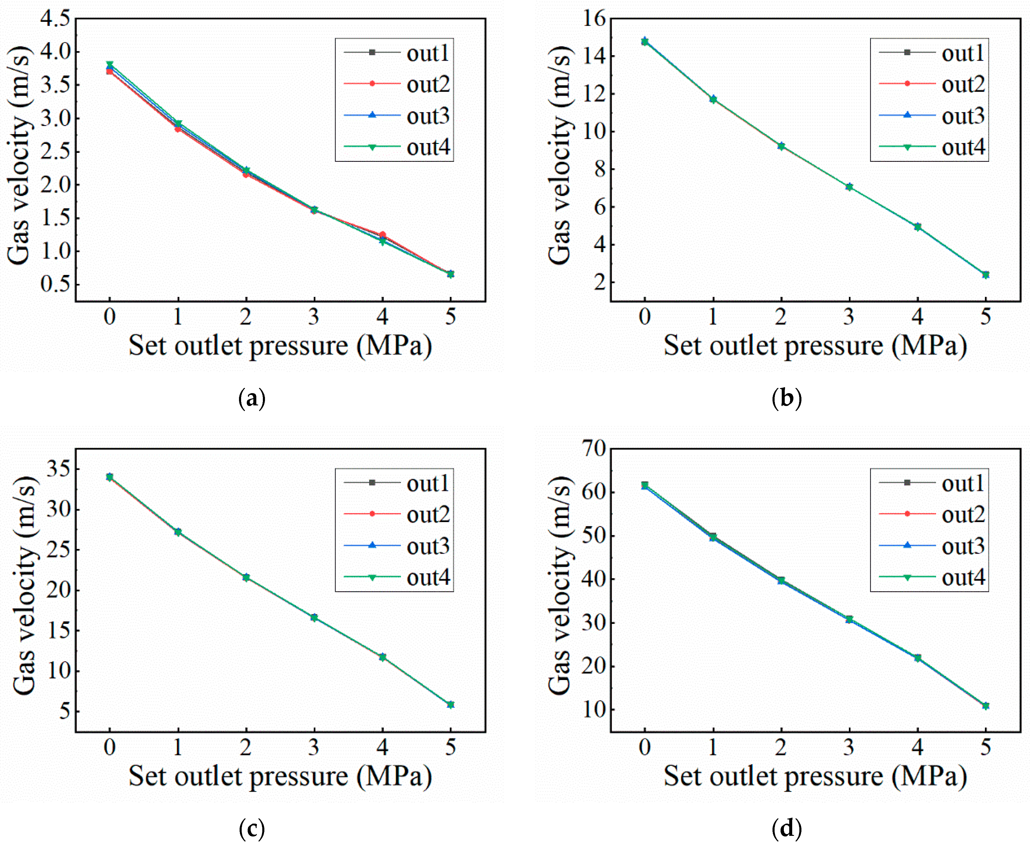
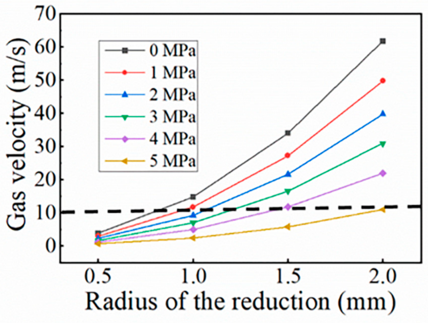
4.2.1. Controlling the Operation Pressure and Gas Velocity in Sampling Branches
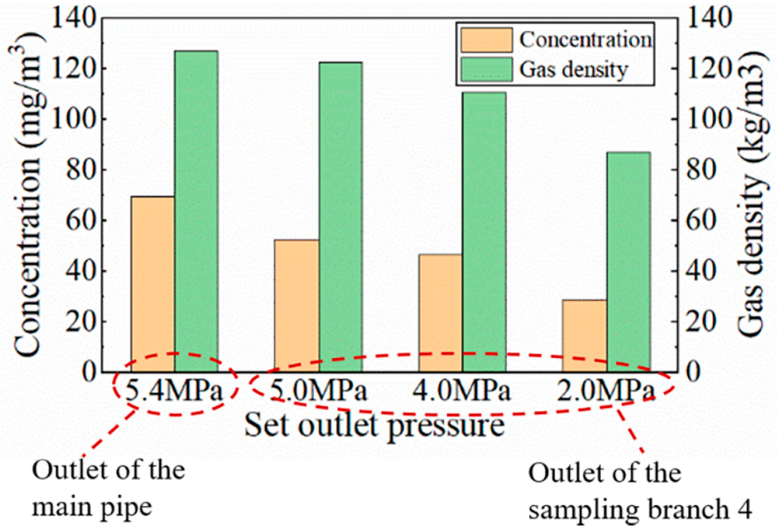
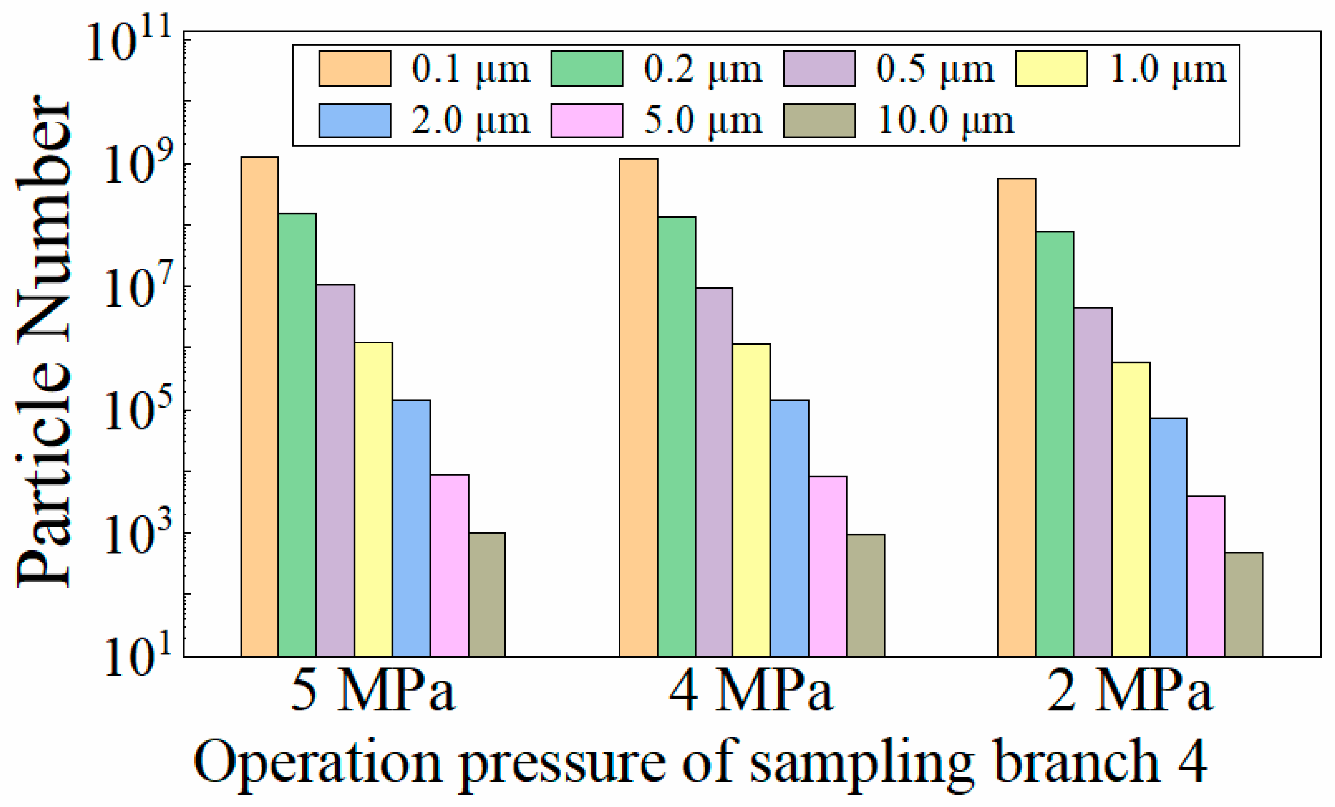
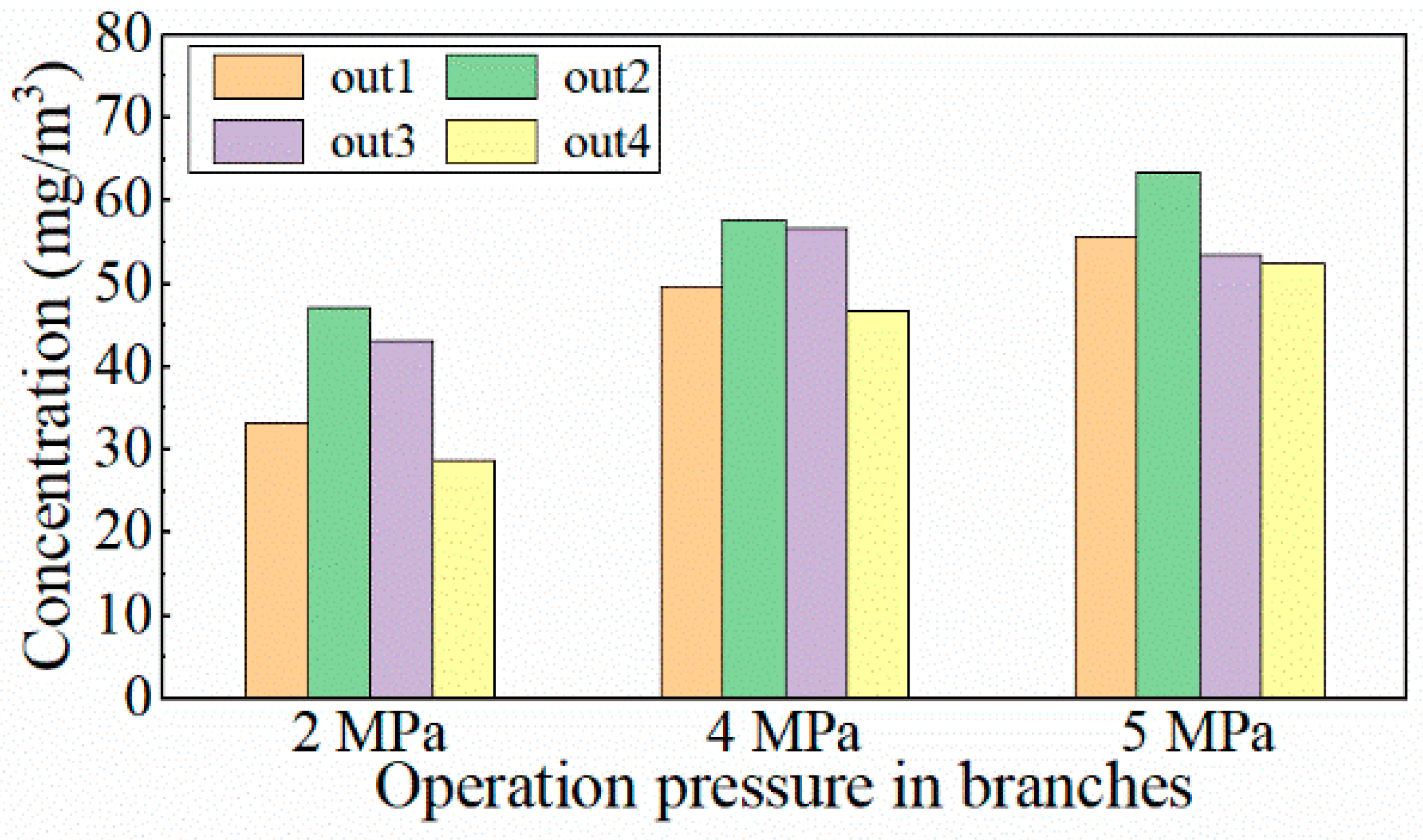
4.2.2. Influence of the Sampling Operating Pressure
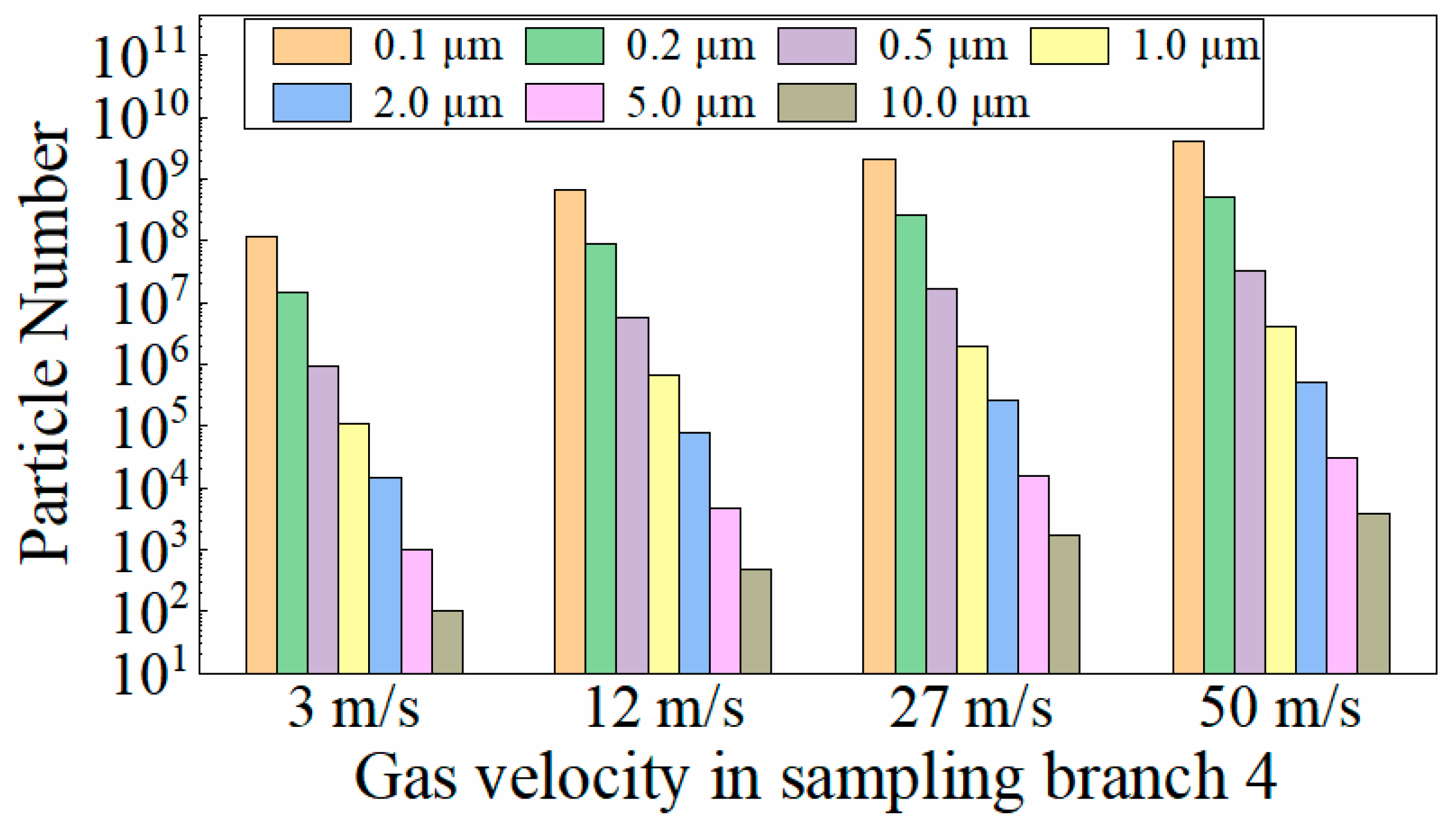
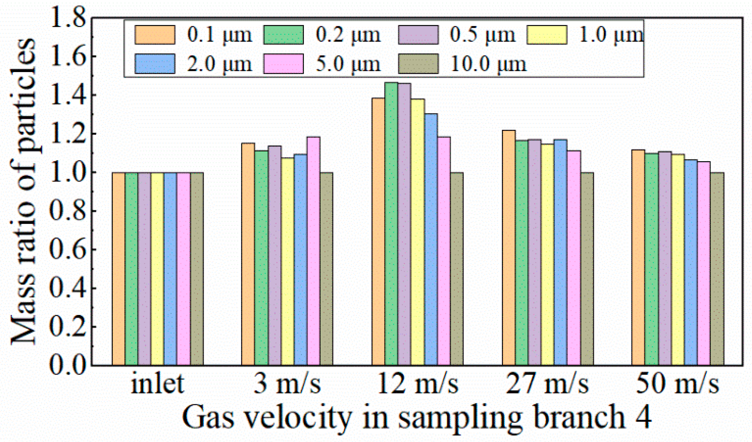
4.2.3. Influence of Sampling Velocity
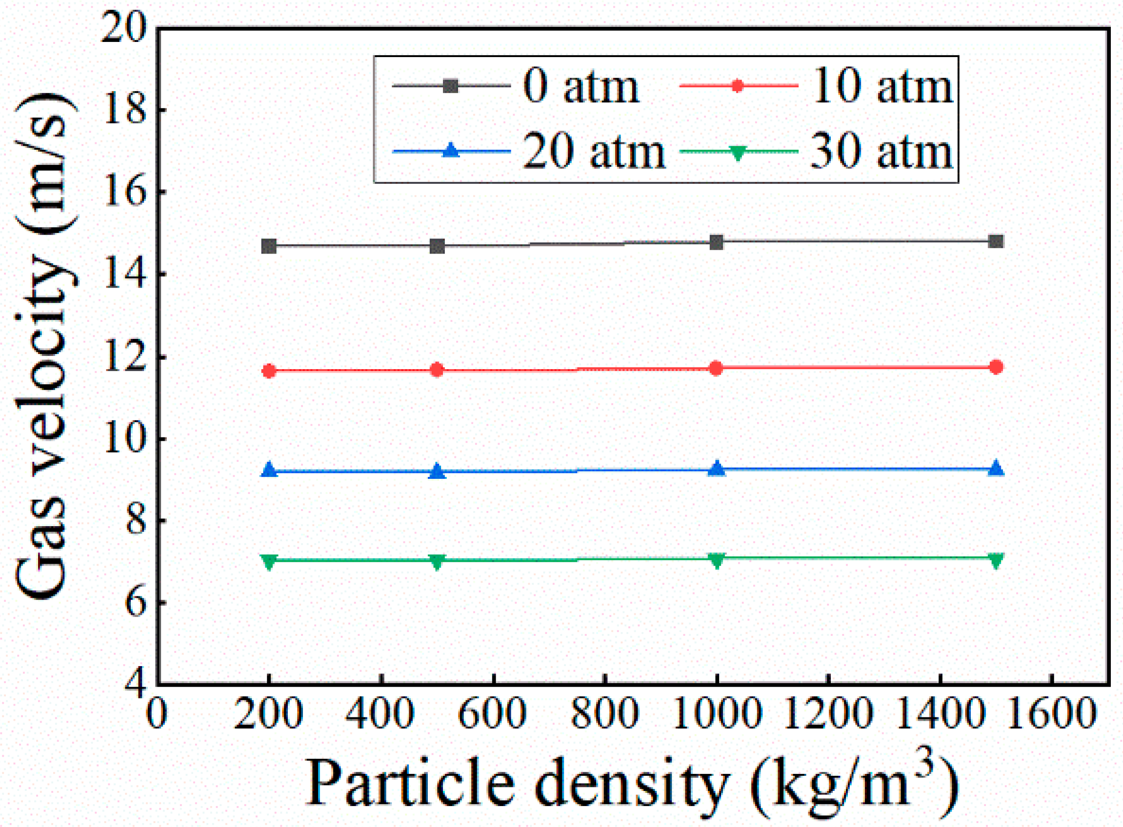
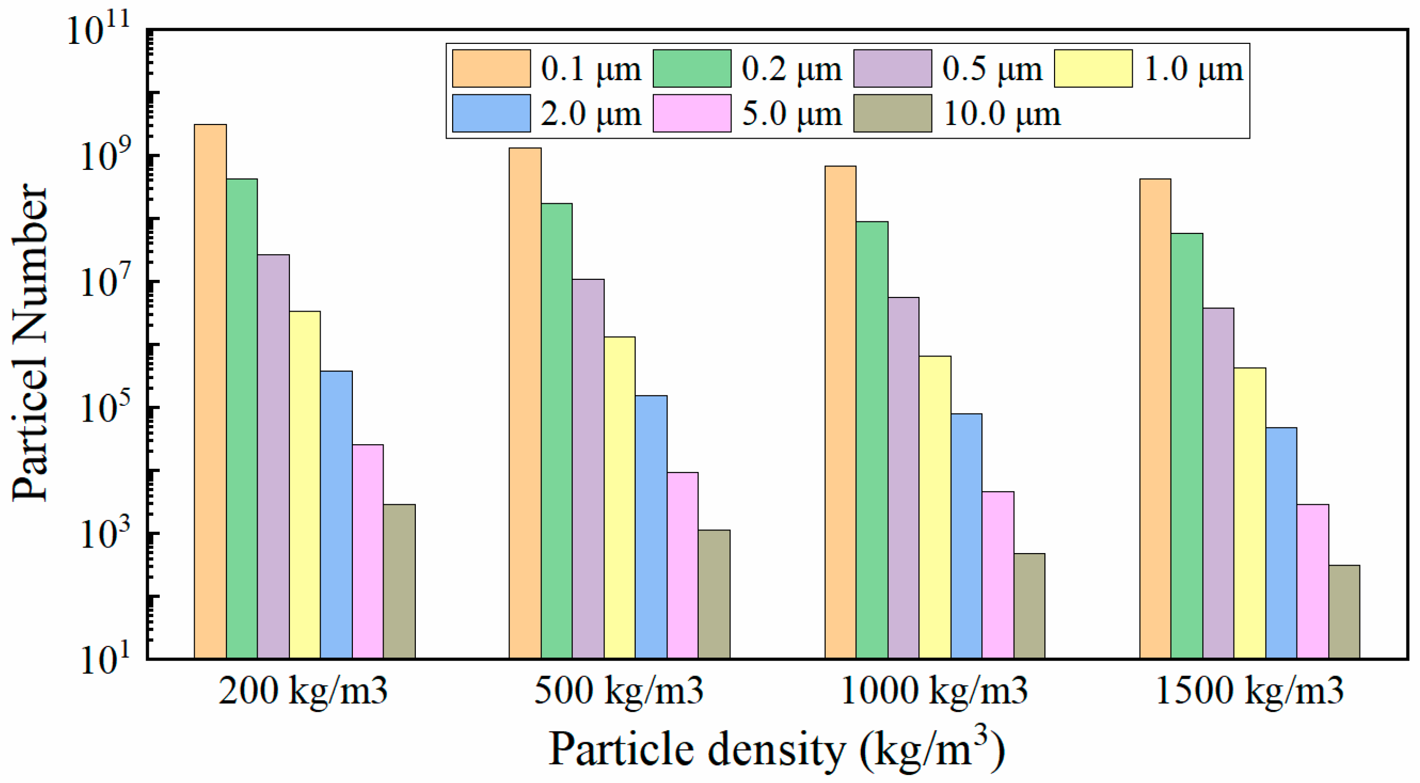
4.3. Influence of Particle Density on Particle Parameters
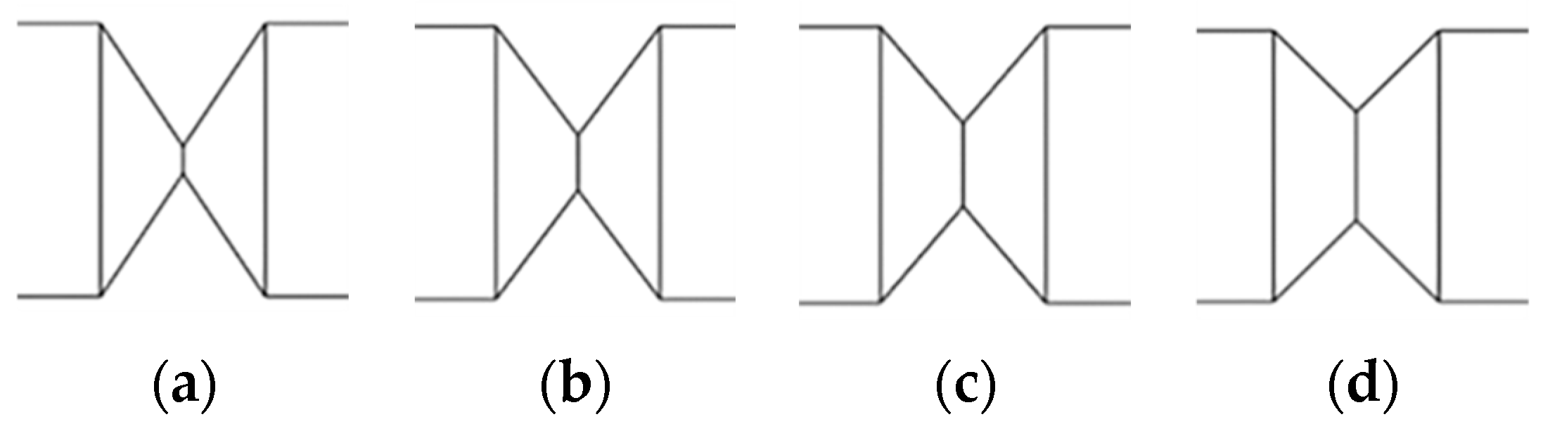
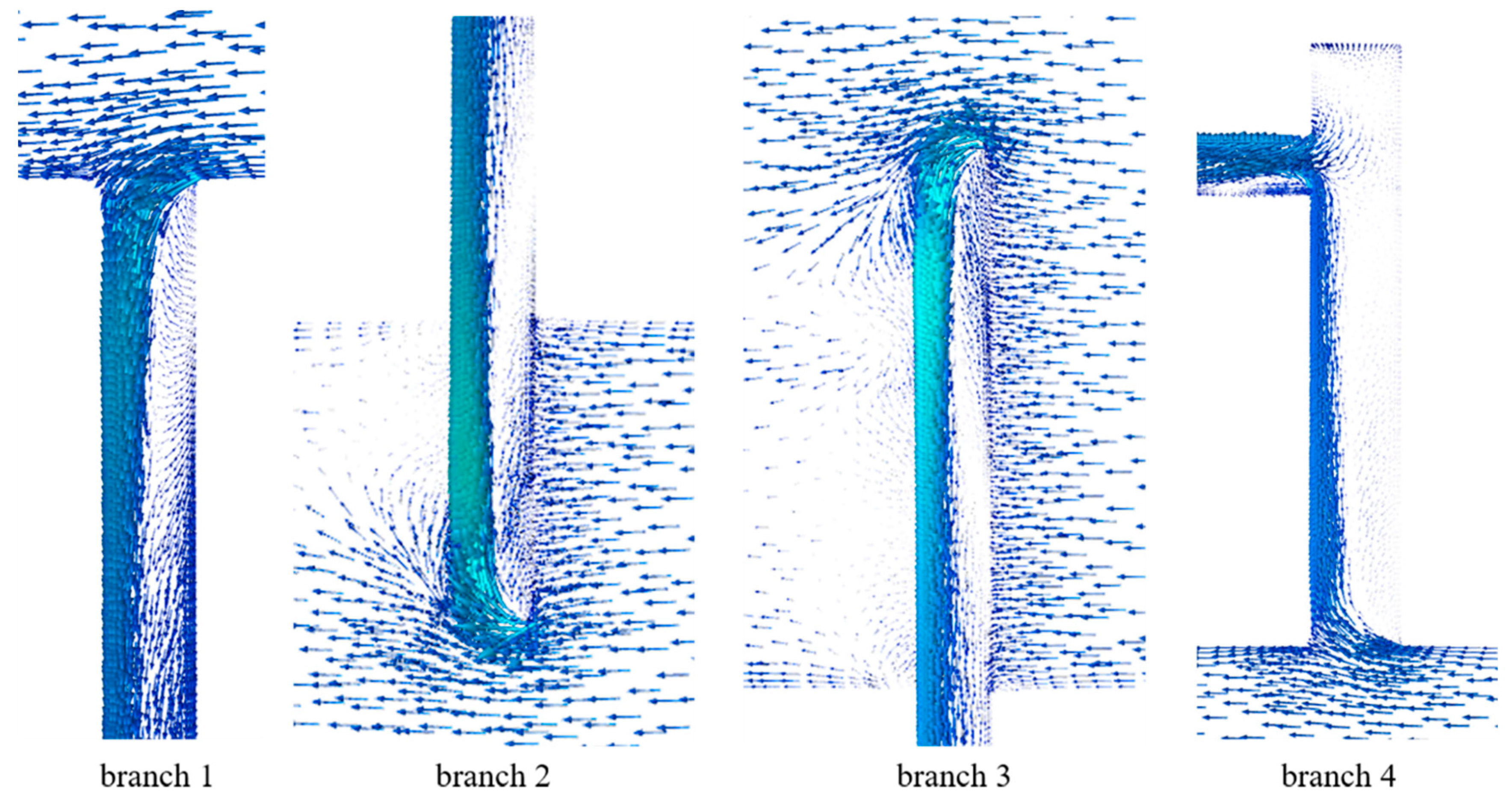
4.4. Influence of the Structure of Sample Branches
5. Conclusions
- The critical diameter at which particles are affected by gravity is 100 μm. For particles smaller than 100 μm, the effect of gravity on their movement in the horizontal pipe can be ignored.
- The operating pressure of the sampling branch has a significant impact on the particle mass concentration, and the particle mass concentration measurement results need to be converted by gas density to obtain the true value in the main pipe. Both sampling operating pressure and sampling gas velocity have little effect on particle size distribution.
- The particle density has little impact on the sampling system, indicating that measurement deviations in sampling are not related to the type of liquid.
- The number of particles in branches inserted into the main pipe is slightly higher than in those without interpolation, but overall, the design of the sampling branches does not cause significant sampling errors.
Author Contributions
Funding
Data Availability Statement
Acknowledgments
Conflicts of Interest
Nomenclature
| CFD | Computational Fluid Dynamics |
| DPM | Discrete Phase Model |
| D | particle diameter |
| F | volume force |
| Gb | buoyancy terms |
| Gk | generation of k due to mean velocity gradients |
| Gω | generation of ω |
| P | pressure |
| R | reduction radius |
| Sk | user-defined source terms |
| ST | viscous dissipation term |
| T | time |
| T | temperature |
| U | velocity components in x direction |
| V | velocity components in y direction |
| W | velocity components in z direction |
| Yk | dissipation of k due to turbulence respectively |
| Yω | dissipation of ω due to turbulence respectively |
| ρ | density |
| τ | viscous stress |
| K | turbulence kinetic energy |
| Ω | specific dissipation rate |
| Γk | effective diffusivities of k |
| Γω | effective diffusivities of ω |
References
- Eyvazi, M.; Asaadi, F.; Akhbarifar, S.; Yousefi, M.R.; Shirvani, M.; Hashemabadi, S.H.; Rezaei, A.K. CFD simulation of a spiral-channel dust separator for removal of black powder from natural gas pipelines. Chem. Eng. Res. Des. 2023, 199, 192–204. [Google Scholar] [CrossRef]
- Torres, L.F.; Damascena, M.A.; Alves, M.M.A.; Santos, K.S.; Franceschi, E.; Dariva, C.; Barros, V.A.; Melo, D.C.; Borges, G.R. Use of near-infrared spectroscopy for the online monitoring of natural gas composition (hydrocarbons, water and CO2 content) at high pressure. Vib. Spectrosc. 2024, 131, 103653. [Google Scholar] [CrossRef]
- Xiong, W.; Zhang, L.-H.; Zhao, Y.-L.; Hu, Q.-Y.; Tian, Y.; He, X.; Zhang, R.-H.; Zhang, T. Prediction of the viscosity of natural gas at high temperature and high pressure using free-volume theory and entropy scaling. J. Pet. Sci. 2023, 20, 3210–3222. [Google Scholar] [CrossRef]
- Hadidi, A. A novel energy recovery and storage approach based on turbo-pump for a natural gas pressure reduction station. J. Clean. Prod. 2024, 449, 141625. [Google Scholar] [CrossRef]
- Ferrario, F.; Busini, V. Statistical analysis of modelling approaches for CFD simulations of high-pressure natural gas releases. Results Eng. 2024, 21, 101770. [Google Scholar] [CrossRef]
- Taha, W.; Abou-Khousa, M.; Haryono, A.; Alshehhi, M.; Al-Wahedi, K.; Al-Durra, A.; Alnabulsieh, I.; Daoud, M.; Geuzebroek, F.; Faraj, M.; et al. Field demonstration of a microwave black powder detection device in gas transmission pipelines. J. Nat. Gas Sci. Eng. 2020, 73, 103058. [Google Scholar] [CrossRef]
- Almara, L.M.; Wang, G.-X.; Prasad, V. Conditions and thermophysical properties for transport of hydrocarbons and natural gas at high pressures: Dense phase and anomalous supercritical state. Gas Sci. Eng. 2023, 117, 205072. [Google Scholar] [CrossRef]
- Kharoua, N.; Alshehhi, M.; Khezzar, L.; Filali, A. CFD prediction of Black Powder particles’ deposition in vertical and horizontal gas pipelines. J. Pet. Sci. Eng. 2017, 149, 822–833. [Google Scholar] [CrossRef]
- Filali, A.; Khezzar, L.; Alshehhi, M.; Kharoua, N. A One-D approach for modeling transport and deposition of Black Powder particles in gas network. J. Nat. Gas Sci. Eng. 2016, 28, 241–253. [Google Scholar] [CrossRef]
- Abou-Khousa, M.; Al-Durra, A.; Al-Wahedi, K. Microwave Sensing System for Real-Time Monitoring of Solid Contaminants in Gas Flows. IEEE Sens. J. 2015, 15, 5296–5302. [Google Scholar] [CrossRef]
- Khan, T.S.; Alshehhi, M.; Stephen, S.; Khezzar, L. Characterization and preliminary root cause identification of black powder content in a gas transmission network—A case study. J. Nat. Gas Sci. Eng. 2015, 27, 769–775. [Google Scholar] [CrossRef]
- Zhang, H.; Zheng, Q.; Yu, D.; Lu, N.; Zhang, S. Numerical simulation of black powder removal process in natural gas pipeline based on jetting pig. J. Nat. Gas Sci. Eng. 2018, 58, 15–25. [Google Scholar] [CrossRef]
- Seyfi, S.; Mirzayi, B.; Seyyedbagheri, H. CFD modeling of black powder particles deposition in 3D 90-degree bend of natural gas pipelines. J. Nat. Gas Sci. Eng. 2020, 78, 103330. [Google Scholar] [CrossRef]
- Khan, T.S.; Al-Shehhi, M.S. Review of black powder in gas pipelines—An industrial perspective. J. Nat. Gas Sci. Eng. 2015, 25, 66–76. [Google Scholar] [CrossRef]
- Xiong, Z.; Ji, Z.; Wu, X.; Chen, Y.; Chen, H. Experimental and numerical simulation investigations on particle sampling for high-pressure natural gas. Fuel 2008, 87, 3096–3104. [Google Scholar] [CrossRef]
- Azadi, M.; Mohebbi, A.; Scala, F.; Soltaninejad, S. Experimental study of filtration system performance of natural gas in urban transmission and distribution network: A case study on the city of Kerman, Iran. Fuel 2011, 90, 1166–1171. [Google Scholar] [CrossRef]
- Azadi, M.; Mohebbi, A.; Soltaninejad, S.; Scala, F. A case study on suspended particles in a natural gas urban transmission and distribution network. Fuel Process. Technol. 2012, 93, 65–72. [Google Scholar] [CrossRef]
- Meyer, J.; Umhauer, H.; Reuter, K.; Schiel, A.; Kasper, G.; Förster, M. Concentration and size measurements of fly ash particles from the clean gas side of a pressurised pulverised coal combustion test facility. Powder Technol. 2008, 180, 57–63. [Google Scholar] [CrossRef]
- Malm, W.C.; Day, D.E. Estimates of aerosol species scattering characteristics as a function of relative humidity. Atmos. Environ. 2001, 35, 2845–2860. [Google Scholar] [CrossRef]
- Gebharta, K.A.; Copelandb, S.; Malmc, W.C. Diurnal and seasonal patterns in light scattering, extinction, and relative humidity. Atmos. Environ. 2001, 35, 5177–5191. [Google Scholar] [CrossRef]
- Chen, D.-R.; Pui, D.Y.H. Numerical and experimental studies of particle deposition in a tube with a conical contraction-Laminar flow regime. J. Aerosol Sci. 1995, 26, 563–574. [Google Scholar] [CrossRef]
- Chuah, T.G.; Gimbun, J.; Choong, T.S.Y. A CFD study of the effect of cone dimensions on sampling aerocyclones performance and hydrodynamics. Powder Technol. 2006, 162, 126–132. [Google Scholar] [CrossRef]
- Li, H.; Wang, S.; Chen, X.; Xie, L.; Shao, B.; Ma, Y. CFD-DEM simulation of aggregation and growth behaviors of fluid-flow-driven migrating particle in porous media. Geoenergy Sci. Eng. 2023, 231, 212343. [Google Scholar] [CrossRef]
- Ponzini, R.; Da Vià, R.; Bnà, S.; Cottini, C.; Benassi, A. Coupled CFD-DEM model for dry powder inhalers simulation: Validation and sensitivity analysis for the main model parameters. Powder Technol. 2021, 385, 199–226. [Google Scholar] [CrossRef]
- Stosiak, M.; Zawiślak, M.; Nishta, B. Studies of Resistances of Natural Liquid Flow in Helical and Curved Pipes. Pol. Marit. Res. 2018, 25, 123–130. [Google Scholar] [CrossRef]
- Karpenko, M.; Bogdevičius, M. Investigation of Hydrodynamic Processes in the System—“Pipeline-Fittings”. In Transbaltica XI: Transportation Science and Technology; Springer International Publishing: New York, NY, USA, 2019. [Google Scholar]
- Zeng, Y.; Ming, P.; Li, F.; Zhang, H. Thermal hydraulic characteristics of spiral cross rod bundles in a lead-bismuth-cooled fast reactor. Ann. Nucl. Energy. 2022, 167, 108850. [Google Scholar] [CrossRef]
- Liu, J.; Guan, X.; Yang, N. Bubble-induced turbulence in CFD simulation of bubble columns. Part I: Coupling of SIT and BIT. Chem. Eng. Sci. 2023, 270, 118528. [Google Scholar] [CrossRef]
- Dyck, N.J.; Parker, M.J.; Straatman, A.G. The impact of boundary treatment and turbulence model on CFD simulations of the Ranque-Hilsch vortex tube. Int. J. Refrig. 2022, 141, 158–172. [Google Scholar] [CrossRef]
- Jubaer, H.; Afshar, S.; Xiao, J.; Chen, X.D.; Selomulya, C.; Woo, M.W. On the effect of turbulence models on CFD simulations of a counter-current spray drying process. Chem. Eng. Res. Des. 2019, 141, 592–607. [Google Scholar] [CrossRef]
- Aounallah, M.; Addad, Y.; Benhamadouche, S.; Imine, O.; Adjlout, L.; Laurence, D. Numerical investigation of turbulent natural convection in an inclined square cavity with a hot wavy wall. Int. J. Heat Mass Transfer. 2007, 50, 1683–1693. [Google Scholar] [CrossRef]
- Rocha, P.A.C.; Rocha, H.H.B.; Carneiro, F.O.M.; Da Silva, M.E.V.; Bueno, A.V. k–ω SST (shear stress transport) turbulence model calibration: A case study on a small scale horizontal axis wind turbine. Energy 2014, 65, 412–418. [Google Scholar] [CrossRef]
- Eça, L.; Hoekstra, M. Numerical aspects of including wall roughness effects in the SST k–ω eddy-viscosity turbulence model. Comput. Fluids. 2011, 40, 299–314. [Google Scholar] [CrossRef]
- Tan, D.; Gan, Q.; Tao, Y.; Ji, B.; Luo, H.; Li, A.; Duan, J. Effects of axial misalignment welding defects on the erosive wear of natural gas piping. Eng. Fail. Anal. 2024, 158, 107972. [Google Scholar] [CrossRef]


| Branch | Diameter (mm) | Length (mm) | Insertion Length (mm) |
|---|---|---|---|
| 1 | 10 | 200 | No insertion |
| 2 | 10 | 200 | 37.5 |
| 3 | 10 | 200 | 75 |
| 4 | 15/10 | 100/200 | No insertion |
| Parameter | Unit | Value |
|---|---|---|
| Operating pressure | MPa | 5.4 |
| Operating temperature | K | 300 |
| Main pipe diameter | mm | 300 |
| Main pipe length | mm | 1000 |
| Sampling branch diameters | mm | 10 |
| Gas phase | - | Natural gas |
| Gas phase density | kg/m3 | Ideal gas |
| Gas phase viscosity | kg/(m·s) | 1.7894 × 10⁻⁵ |
| Gas phase velocity in the main pipe | m/s | 10 |
| Particle | - | Water |
| Particle diameter | μm | 0.1, 0.2, 0.5, 1.0, 2.0, 5.0, 10.0 |
| Particle density | kg/m3 | 1000 |
| Released particle mass concentration | kg/m3 | 70 |
| Released particle velocity | m/s | 10 |
| Grid | Cell Number | Surface Mesh Size (mm) | ||
|---|---|---|---|---|
| Main Pipe | Sampling Branches | Reduction | ||
| Coarse grid | 783,863 | 4.5 | 1.2 | 0.5 |
| Medium-sized grid | 1,196,035 | 4 | 1 | 0.4 |
| Fine grid | 1,429,798 | 3.8 | 0.8 | 0.3 |
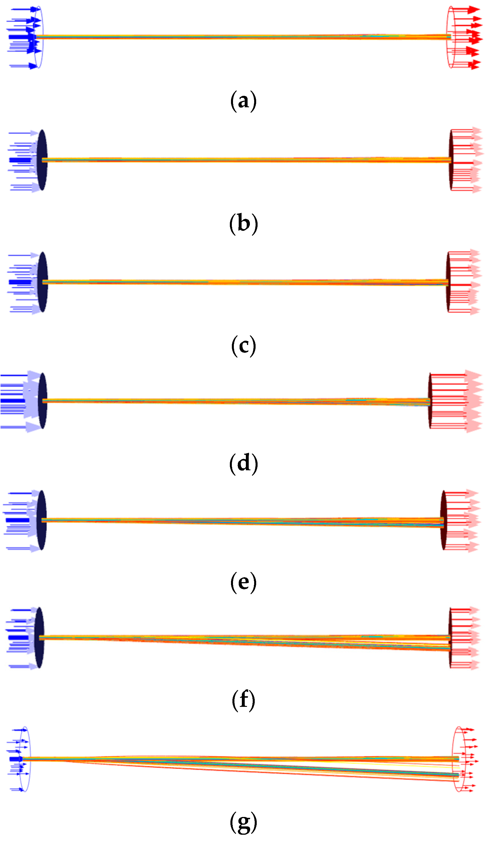
| Case | Incident Particle Group Sizes (μm) |
|---|---|
| a | 0.1, 0.5, 1, 2, 5, 10 |
| b | 0.1, 0.5, 1, 2, 5, 10, 20 |
| c | 0.1, 0.5, 1, 2, 5, 10, 50 |
| d | 0.1, 0.5, 1, 2, 5, 10, 100 |
| e | 0.1, 0.5, 1, 2, 5, 10, 200 |
| f | 0.1, 0.5, 1, 2, 5, 10, 500 |
| g | 0.1, 0.5, 1, 2, 5, 10, 1000 |
| Parameter | Unit | Value |
|---|---|---|
| Main pipe diameter | mm | 300 |
| Main pipe length | mm | 2000 |
| Operating pressure | MPa | 5.4 |
| Gas phase | - | Ideal gas |
| Inlet velocity of the gas phase | m/s | 10 |
| Particle | - | Water |
| Particle density | kg/m3 | 1000 |
| Diameter of particle inlet | mm | 20 |
| Inlet concentration of each size of particles | mg/m3 | 10 |
Disclaimer/Publisher’s Note: The statements, opinions and data contained in all publications are solely those of the individual author(s) and contributor(s) and not of MDPI and/or the editor(s). MDPI and/or the editor(s) disclaim responsibility for any injury to people or property resulting from any ideas, methods, instructions or products referred to in the content. |
© 2024 by the authors. Licensee MDPI, Basel, Switzerland. This article is an open access article distributed under the terms and conditions of the Creative Commons Attribution (CC BY) license (https://creativecommons.org/licenses/by/4.0/).
Share and Cite
Wu, M.; Chen, Y.; Liu, Q.; Xiao, L.; Fan, R.; Li, L.; Xiao, X.; Sun, Y.; Yan, X. CFD Research on Natural Gas Sampling in a Horizontal Pipeline. Energies 2024, 17, 3985. https://doi.org/10.3390/en17163985
Wu M, Chen Y, Liu Q, Xiao L, Fan R, Li L, Xiao X, Sun Y, Yan X. CFD Research on Natural Gas Sampling in a Horizontal Pipeline. Energies. 2024; 17(16):3985. https://doi.org/10.3390/en17163985
Chicago/Turabian StyleWu, Mingou, Yanling Chen, Qisong Liu, Le Xiao, Rui Fan, Linfeng Li, Xiaoming Xiao, Yongli Sun, and Xiaoqin Yan. 2024. "CFD Research on Natural Gas Sampling in a Horizontal Pipeline" Energies 17, no. 16: 3985. https://doi.org/10.3390/en17163985