A Techno-Economic Assessment of DC Fast-Charging Stations with Storage, Renewable Resources and Low-Power Grid Connection

Abstract

The growing demand for high-power DC fast-charging (DCFC) stations for electric vehicles (EVs) is expected to lead to increased peak power demand and a reduction in grid power quality. To maximize the economic benefits and station utilization under practical constraints set by regulatory authorities, utilities and DCFC station operators, this study explores and provides methods for connecting DCFC stations to the grid, employing low-power interconnection rules and distributed energy resources (DERs). The system uses automotive second-life batteries (SLBs) and photovoltaic (PV) systems as energy buffer and local energy resources to support EV charging and improve the station techno-economic feasibility through load shifting and charge sustaining. The optimal sizing of the DERs and the selection of the grid interconnection topology is achieved by means of a design space exploration (DSE) and exhaustive search approach to maximize the economic benefits of the charging station and to mitigate high-power demand to the grid. Without losing generality, this study considers a 150 kW DCFC station with a range of DER sizes, grid interconnection specifications and related electricity tariffs of American Electric Power (AEP) Ohio and the Public Utility Commission of Ohio (PUCO). Various realistic scenarios and strategies are defined to account for the interconnection requirements of the grid to the DCFC with DERs. The system’s techno-economic performance over a ten-year period for different scenarios is analyzed and compared using a multitude of metrics. The results of the analysis show that the the integration of DERs in DCFC stations has a positive impact on the economic value of the investment when compared to traditional installations.

1. Introduction

Electric vehicle (EV) DC fast-charging (DCFC) stations have the benefit of providing faster charging times to EV customers and reducing range anxiety [1,2,3,4]. However, the integration of DCFC stations into the electric grid brings a number of challenges, including rising energy demand and peak power requests, the need for grid upgrades, the potential decline in grid reliability, the degradation of power quality and increased losses [4,5,6,7]. To address these challenges, utilities and grid operators may need to upgrade substations’ transformers, install power factor correction equipment, and implement advanced control systems to mitigate the impact of impulsive EV charging events [8].

Traditional DCFCs are often interconnected to the grid at the medium-voltage (MV) level due to high power requests; this requires distribution-level transformers to convert MV to low voltage (LV) for the DCFC equipment [1,4]. In various reports and studies, it is shown that high load requirements from simultaneous charging of EVs might not be supplied by the available distribution-level transformers, and it is most likely that upgrades are required to accommodate DCFC stations [9]. According to the EPIC project report by PG&E [10], of the 300 one-mile radius locations identified on the map for EV charging station locations, only about 45% of the locations had available capacity for more than 50 kW. While this may allow for the addition of a few 50 kW chargers to existing transformers, additional hundreds of kW of power would likely require an upgraded or a separate transformer off the distribution line [11,12]. In some cities, the government has mandated the installation of distribution-level transformers for DCFC stations to reduce the load on existing infrastructures [13,14]. Other challenges that are limiting the DCFC infrastructure’s readiness level include legislative requirements, capital investments, high power availability and building regulations and codes [15]. As an example, the direct connection of DCFC stations to the LV distribution grid can reduce the capital and operation costs of the investment by limiting the installation of new distribution transformers [2,16,17,18]. However, this approach may not be feasible in all situations, as the LV transformers may not be able to handle the increased demand for power caused by DCFC stations and may require upgrades to accommodate the additional load.

One of the most common solutions to reduce the impact of DCFC stations on the grid is the integration of distributed energy resources (DERs) and smart management control of supply and demand [19,20,21,22]. There are various financial advantages of the optimal management of the power requested by the charging stations, according to [9,23], including the reduction of energy and power (demand) costs. In [19], the authors compared the technical and economic viability of operating DCFC stations with and without energy buffers, such as batteries, and it was found that the installation of local storage improved grid stability and reduced power demand on the grid. There are also some commercially available DCFC stations that use energy storage systems. Freewire Boost EV charger, Powerstar Battery Buffered EV Charger and ADSTec Energy EV Charger are some of the examples [24,25,26]. Microgrid approaches have attracted large interest since they combine renewable energy sources like photovoltaics (PVs) for energy production and energy storage systems (ESSs) for load shifting. Li-Ion batteries (LIBs) are an excellent option for ESSs with PVs due to their many advantages, such as long life, low auto-discharge, availability, energy and power density. Some of the following advantages have been reported in the available literature for DCFC stations with integrated DERs [19,27,28,29,30]:

• Faster discharge rates of stationary batteries based on LIBs allow direct charging of EVs through ESSs, heavily reducing the power request on the grid.
• The longer life cycle of PVs and LIBs reduces the maintenance of the station and increases the longevity of the project.
• PVs can supply energy from solar irradiation that can be stored in ESSs, and due to the higher energy density of LIBs, higher energy can be stored as compared to other storage options.
• Charging stationary batteries from the grid at lower power and electricity rates can reduce the demand and energy charges and then the cost of DCFC events to the final customer.
• Bidirectional flow of power through ESSs allows participation in grid ancillary services.
• Energy storage can take advantage of time-of-use energy rates.
• There are also incentives and tax rebates in some states which can lower the cost of the investment in both residential and commercial applications.

Numerous research papers are available that focus on minimizing the effects of DCFC stations on the grid owing to high charging loads and appropriately sizing DERs to optimize the economic benefits. In order to minimize the grid impact of DCFC stations, [31] seeks to identify the optimum design of DERs. Sizing is carried out using a cost–benefit analysis (CBA) of the installation fee, battery life and electricity cost. Refs. [32,33] present an economic analysis using net present value (NPV) to size the PV and ESS for a DCFC station. A particle swarm optimization problem was formulated based on a financial model that comprises the grid tariff, PV availability, EV demand and prices for EV charging to size the battery packs and PV modules [34].

An extensive literature review and analysis revealed that while there are a lot of studies contributing to properly sizing DERs for DCFCs, there are significant aspects of using DERs in charging stations that are not outlined in the current literature. Below are some of the limitations that are found in the current literature:

• Many scientific studies do not provide practical and realistic methods to integrate the DERs in a DCFC station. In many of these research studies ([6,18,31,32,33,34,35]), the authors do not consider how the station will be connected to the grid with respect to the grid power/voltage levels and interconnection requirements, including the distribution transformer.
• The reduction of energy and power requirements from the grid corresponds to different energy and demand charges that are often not considered in the literature. In [18], the authors propose to connect the battery system to the DC-DC bus and the AC-DC converter is connected to the LV of the DCFC. The power of connection to the grid is significantly high, which does not reduce the impact of EV load on the grid. An optimum design of a charging station with a DC bus and storage system is presented in [17], but the grid connection size is reduced by considering the average rather than the peak power demand. A recent report by the Rocky Mountain Institute analyzes all charging events at 230 EVgo DCFC stations in the state of California during 2016 and highlights that the high cost of demand charges is a significant barrier to public DCFC network operators’ financial viability [36]. Other studies also show that demand charges have the highest cost-to-ratio in the operating cost structure, which results in poor rates of earnings and delayed returns on investments. Demand charges play a significant role in the operational cost weighting of the EV charging station and have been considered as an important parameter in this study to improve the station finances.
• LIBs report degradation in performance due to usage and time [28,37,38]. Over the station lifetime, the performance of an integrated ESS eventually deteriorates, causing reduced station performance and ultimately leading to the replacement of the stationary battery packs. Very few researchers use battery degradation models and replacements of batteries to analyze the technical or economical performance of a DCFC station. One of the recent studies [30] presents an optimization approach to size the battery packs and PVs based on the NPV of the station. It considers basic cyclic aging based on battery usage but does not include the actual degradation characteristics of the battery due to thermal, electrical and time effects.
• In many of the literature works, it is found that the use of EV load profiles has been considered to be the averaged data or aggregated load for the station [30,32,35,39,40]. From the analysis in [41], it is found that the average-based power profile corresponds to less stress on the stationary storage due to the lower power requirements and the lower number of daily cycles. Using event-based profiles lead to a realistic utilization of the batteries and PV system which captures the realistic behavior and performance of the DCFC station using DERs.

This research study aims at bridging the gaps in the literature and existing solutions by developing a realistic techno-economic analysis over a 10-year time period to demonstrate the feasibility of DCFC stations with integrated second-life batteries (SLBs) and photovoltaic (PV) systems for low-power grid connection. This can potentially reduce and mitigate the required grid infrastructure investment to enable more DCFC stations while reducing the CAPEX and OPEX costs of DCFC stations. The solutions analyzed in this work are compared with a DCFC station project focusing on traditional interconnection requirements and not DERs. The statutory, utility and station requirements are assessed with a design space exploration (DSE) based on exhaustive search to maximize the station’s economics and reduce the grid burden. Several realistic interconnection options are considered, and for each one of these options, an optimized DER sizing is carried out. To evaluate the finances of the charging station at the end of life (EOL), the net present value (NPV) as an economic assessment parameter is selected, which considers the yearly cash flow, inflation, power of money and discount factor as its inputs. An electro-thermal model of the DCFC station including DERs is used to estimate the performance of the investment over its lifetime. These models can assess the need for SLB replacement based on temperature and frequency of use, improving the accuracy of the estimation of the investment value [42]. In order to minimize operating costs, an energy management controller was defined to maximize the use of PV energy for SLB and EV charging or station self-consumption. Through the net metering service, any PV energy that is not used can be fed to the grid and used later on, allowing an increase in the station’s self-consumption and mitigating ESS size and cycling. Making this research practical and applicable to DCFC installations under various grid scenarios involves being aware of how stations and distributed energy resources (DERs) can be connected to the utility grid. Different possibilities for connecting the planned DCFC station to the grid based on the point of interconnection regulations of AEP Ohio and PUCO are examined in the paper. Hence, the event-based profile from [41] is used in this study to create realistic case scenarios and properly consider the impact of energy and demand charges. Innovative solutions are then compared to a DCFC station based on traditional interconnection and no DERs.

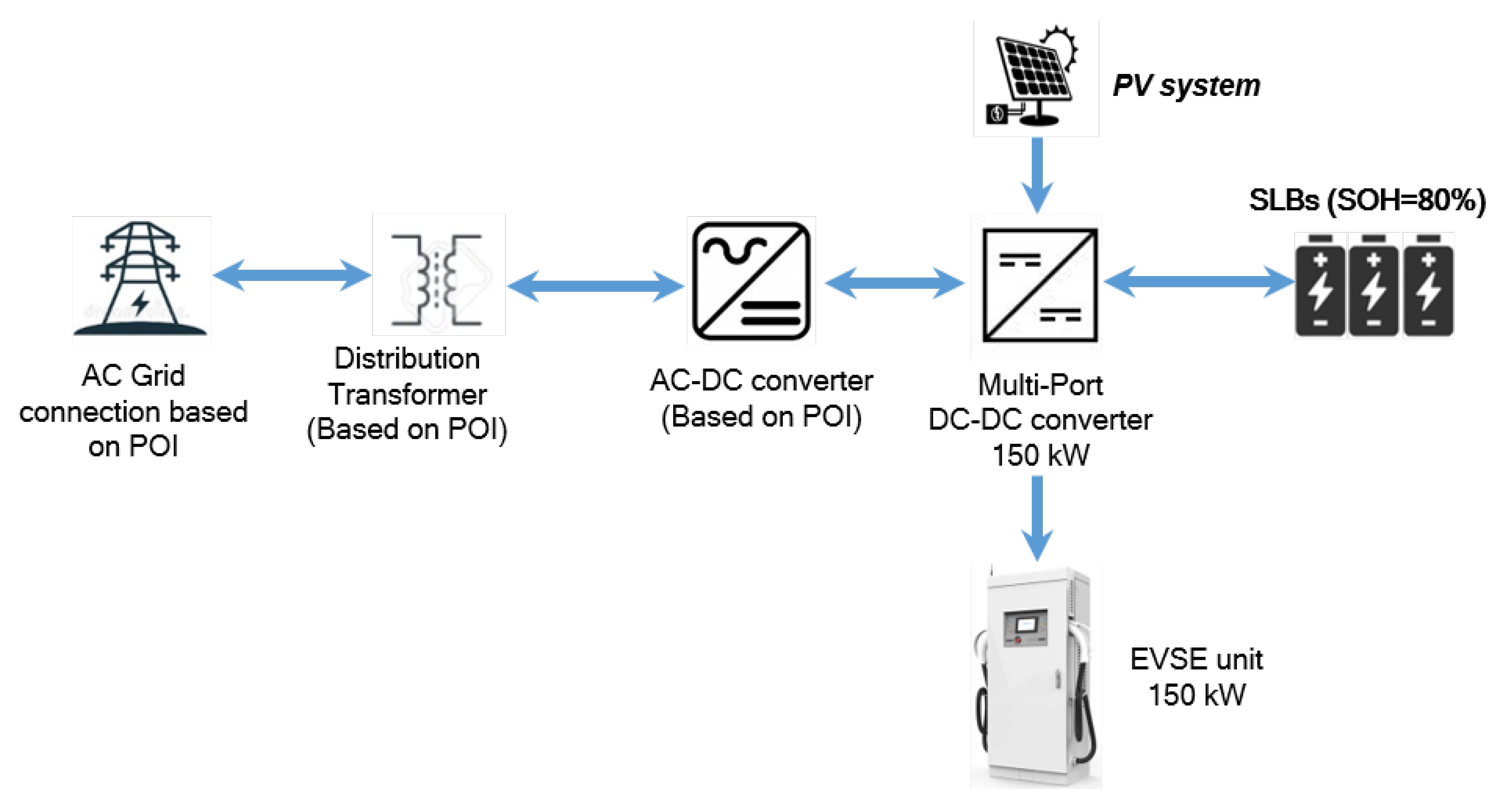
2. DCFC Station Architecture and Modeling

The DCFC station considered in this work includes SLBs and PV systems connected with a low-power bidirectional connection to the grid (point of interconnection or POI). Further, a 150 kW charging station is considered as an example; however, this architecture design can be extended to various power levels of DCFC stations. The proposed architecture is an evolution of the concept proposed in [28,42]. Figure 1 shows the architecture of the proposed DCFC station with its subcomponents and grid interface. The SLBs are connected to the grid using a secondary-distribution-level transformer and a bidirectional AC-DC converter with a maximum power connection from the grid rating POI. The distribution transformer is not considered to be part of the DCFC station when the power of the POI is lower than 120 kW, as defined by [43]. A bidirectional DC-DC converter, rated up to the maximum power of EVs charging, is located on the other side of the SLBs and connects the batteries to the EVs and PV system. The PV is capable of providing power through the DC-DC converters. However, the SLB and grid can have bidirectional power flow. The bidirectional flow with the grid enables additional PV power, more than the station’s self-consumption, to be sent back to the grid (according to the net metering rules [43]). On the EV side, the connection is made using an electric vehicle supply unit (EVSE) and unidirectional power flow. The vehicle-to-grid (V2G) capability is not considered for this study.

An energy management controller (EMC) was developed to prioritize the charging power availability for EV users and maintain the battery’s state of charge (SOC) within safe operating ranges. The energy required by the EVs can be delivered by the stored energy in the SLBs. Additionally, the remaining energy requirement of the EVs can be supplied by two sources, the PV and the grid. Using SLBs as the direct supply of power reduces the power dependence of the EVs on the grid. Further, the SLBs can be charged using the sources of PVs and the grid. The proportion of the power provided by either of the sources is dependent on the availability of solar energy.

To maximize the station’s performance and the economic benefits of the proposed architecture, the interaction of the DERs (SLBs and PVs) and the grid needs to be optimally selected and optimized. A suboptimal configuration could lead to oversizing or undersizing of the sources or DERs, causing economic and energy loss. Design parameters for this work are chosen as the sizes of SLBs ($n_{SLB}$) and PVs ($n_{PV}$) and the grid interconnection power ($P_{POI}$).

This section describes the thermo-electric model of the DCFC station with integrated DERs and the financial model of the investment. This model is used to perform an analysis of the system and related investment over a 10-year time period. The station model receives design inputs along with environmental factors and daily EV demands. Each subsystem outputs the daily energy requirements of the station and its components along with the estimate of the SLB’s state of heath (SOH). The power, energy requirements and SLB replacement factor are given to the economic model that provides daily, monthly and yearly cash flow, which is discussed in a later subsection. Multiple pieces of the literature and data from national labs are used to calibrate all of the subsystem model and economic model parameters.

Then, Section 3 presents a design space exploration technique to optimize the DERs (PV and SLB) for different grid interconnection power levels ($P_{POI}$). For different $P_{POI}$, configurations of battery and PV systems are modeled and assessed in terms of performance and economics to select the optimal configuration. Then, the optimized solutions are compared with a traditional DCFC station with no DERs.

2.1. System Modeling

The architecture of the DCFC station model was inspired by the previous works published in [28,41,42,44,45,46] and was updated for this work. The details of the components with their respective models are given in Table 1. An overview of the system model architecture is shown in Figure 2. The model design is augmented considering a multi-source DCFC station including a grid connection, PV model and SLB packs.

The battery pack model includes electrical, thermal and degradation performance, and it was calibrated experimentally using a Ford Focus EV 2012. The aging method estimates the capacity and internal resistance of the batteries based on the cycle and calendar life using the realistic operating conditions of the battery estimated by the battery electro-thermal model. A thermal management system (TMS) model emulates a liquid cooling system and related control. The battery model was incorporated with a battery management system (BMS) model to keep the battery’s parameters in the safe operating region (voltage, current, temperature, state-of-charge limits) [46]. TMS and BMS were calibrated experimentally using a Ford Focus EV 2012. The battery capacity and internal resistance are degraded overtime on the basis of the current, state of charge and temperature of operation. The model used in this work includes both calendar and cycling aging and is inspired by the empirical aging model reported in [45]. The PV model is based on real solar irradiation and weather data from Columbus, Ohio, in the year 2020 [47], and the PV panel used is a BP 3 SERIES 235 Watt [48]. The EV model acts as a load when EVs are present, while the power converter model provides efficiency based on system power and voltage. All the power converters are modeled using an efficiency map as a function of the processed power. The EV load was modeled as a series of pulses distributed in time and calibrated using field data, as developed in [41]. The grid model outputs the power based on the request from the energy management controller (EMC). The grid’s initial boundary conditions are set up to maintain the system parameters within defined ranges of several predetermined scenarios.

Table 1. Details of the DCFC station model used in this work.

Components	Model Used	References
SLB	Zero-order equivalent circuit model	[28,42]
SLB thermal	Lumped parameter thermal model	[28,42]
SLB BMS	State flow	[46]
SLB aging	Daikin’s battery aging model	[28,42,45]
PV	Five-parameter model	[49]
AC-DC and DC-DC	Efficiency-based model	[41]
EV load	Event-based profile	[41]

Table 1. Details of the DCFC station model used in this work.

Components	Model Used	References
SLB	Zero-order equivalent circuit model	[28,42]
SLB thermal	Lumped parameter thermal model	[28,42]
SLB BMS	State flow	[46]
SLB aging	Daikin’s battery aging model	[28,42,45]
PV	Five-parameter model	[49]
AC-DC and DC-DC	Efficiency-based model	[41]
EV load	Event-based profile	[41]

An EMC is included to enable the proper operation of the station over its lifetime and to ensure that power is readily available for EVs under realistic system constraints. To select the dispatch strategy, the EMC collects the battery information, such as $SOC$, temperature $T_{SLB}$ and voltage $V_{SLB}$, from the SLB model, PV available power $P_{PV}$ and the load request $P_{EV}$ from EVs at time t to define the power reference for SLB, PV and grid ($P_{SLB}$, $P_{PV}$, $P_g$, respectively). The other tasks are to fully utilize the PV energy and maintain the battery SOC within a certain operating range. The EMC operates in such a way as to maintain SLB charging while maximizing PV utilization when EVs are not present at the station. If there is surplus PV energy available, net metering [43] will be used. The SLB charge is allowed only if EVs are not present. The control strategy allows the SLB to be charged through the PV whenever solar irradiation is available. If the PV power is more than the minimum charging power threshold of the SLB $\left(P_{SLB,ch}^m\right)$, all the available PV power is given to the SLB charging and no power is used from the grid. However, if the PV power is less than the charging power threshold $\left(P_{SLB,ch}^m\right)$, the grid supplements the SLB charging up to the minimum charging power of the SLB. Note that $\left(P_{SLB,ch}^m\right)$ varies with the selection of scenarios, as discussed in Section 3, and is considered as the maximum power used from the grid $\left(P_g^M\right)$. When the PV is available and SLB is fully charged (SOC > 95%), the PV residual power is fed into the grid and will be operated in net metering mode. The details of SLB and EV charging controls are given in

Table 2. Control strategies for SLB charging.

SLB	CONTROL
Charging	$P_g$	$P_{PV}$	$P_{SLB}$	$P_{EV}$
Grid only	$P_{POI}$	0	$-P_{SLB,ch}^m$	0
Grid + PV	$P_{POI}$	$P_{MPP}$	$-P_{SLB,ch}^m$	0
PV only	0	$P_{MPP}$	$-P_{PV}$	0
No charging Net metering	$-P_{PV}$	$P_{MPP}$	0	0

and

Table 3. Control strategies for EV charging.

EV	CONTROL
Charging	$P_g$	$P_{PV}$	$P_{SLB}$	$P_{EV}$
SLB only Control A	0	0	$P_{EV}$	>0
SLB + PV Control B	0	$P_{MPP}$	$P_{EV}-P_{MPP}$	>0
Grid + PV + SLB Control C	$P_{POI}$	$P_{MPP}$	$P_{EV}-P_{MPP}-P_{POI}$	>0

, respectively.

For EV and SLB charging mode, the power balance equation is given in (1).

$$P_{SLB}+P_{PV}+P_g=P_{EV}$$

(1)

During EV charging, three types of control strategies for EV charging are considered. These strategies change the dependence on the grid and PV for EV charging and the ways they are used to support SLBs during EV charging:

• Control A: Charge EV only from SLB. In this control strategy, the EVs are directly charged from the SLBs, and no other source is used.
• Control B: Charge EV from SLB and PV. In this control strategy, the PV power, if available, has the priority when an EV requests to be charged with the aim of maximizing the energy from renewable resources. The PV power is equal to the maximum power point $P_{MPP}$ [50]. Then, the remaining power required by the EVs is supplied by the SLB. There is no use of grid energy to charge EVs in this control.
• Control C: Charge EV from SLB, grid and PV. In this control strategy, the PV power, if available, has the priority when an EV requests to be charged with the aim of maximizing the energy from renewable resources. The PV power is equal to the maximum power point $P_{MPP}$. Then, the remaining power required by the EVs is supplied by the SLB and the grid. The grid power supplies the maximum interconnection power $P_{POI}$.

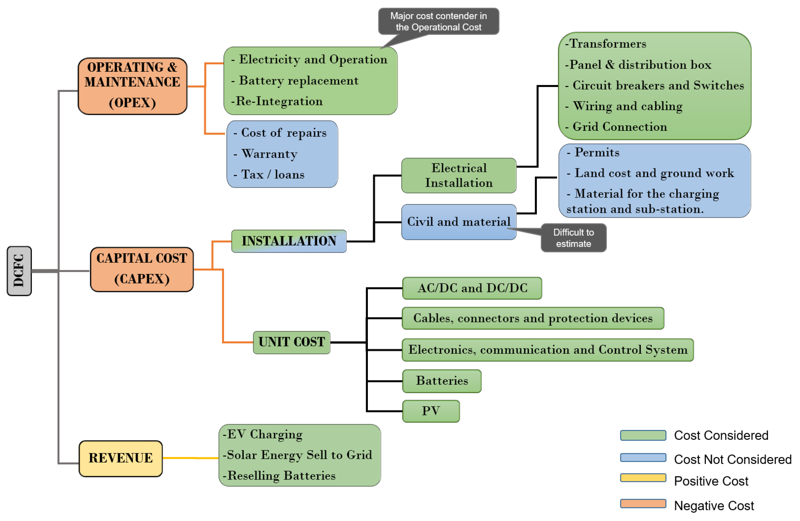
2.2. Economic Modeling

In this subsection, the cost of ownership of the EV DCFC station is evaluated and the economic value of the station is assessed through net present value (NPV) method. The breakdown of the cost structure of owning, maintaining and operating a DCFC station is considered for both the traditional and proposed station models, and these are later compared in Section 4. The costs can be categorized as capital cost (CAPEX), operating cost (OPEX) and revenue. The descriptions of components for the DCFC costs are shown in Figure 3, which includes all major cost components of the proposed DCFC station.

The capital investment cost, or CAPEX, is based on the price of the materials and the cost of their installation related to the DCFC’s components. Because it is challenging to predict the site and land needs, permitting and civil costs are outside the scope of this work. The operational cost, also known as OPEX, is the variable cost that fluctuates with time and consumption depending on how the sources are used, such as the cost of the electricity in terms of energy and power. The cost of charging station maintenance, which primarily consists of need for SLB replacement, is also included. The replacement of PV modules and station maintenance is not taken into account as the components’ and PV life exceeds the project’s total life. Taxes are paid for electricity use and EV charging; warranties and location-based taxes are not taken into account. The station’s expenses are its CAPEX and OPEX costs, while revenue represents cash inflow from the EV charging events and various revenue sources such as solar credits and battery resale earnings.

The cost parameters with their descriptions and references are listed in Table 4, Table 5 and Table 6. A detailed survey of the recent literature and data was performed to accurately evaluate the values of each cost component and for each of the cost categories. The data were collected from a multitude of publications from industry, national laboratories, academia and energy reports.

The balance of system (BOS) is a part of the CAPEX that includes components of an ESS excluding the battery pack’s cost. The segregation is performed from the ESS to cost per unit basis in terms of energy for ESS (USD/kWh) and in terms of power for BOS (USD/kW). BOS includes BMS, thermal management system (TMS), wiring and cabling, connectors isolation system and protection circuits and fire management system (FMS). Repurposing or reintegrating the SLBs also adds cost to the CAPEX value.

The parameters for the demand charges and the electricity charges were referenced from the Ohio Electricity Tariff rules [51]. The values of the bill were normalized to obtain USD/kWh value for the energy or electricity consumption in terms of kWh used and in USD/kW for the demand charges to account for the power in kW used.

The revenues have three contributors, the earnings from EV charging, the earnings from selling the batteries after the end of the project with the energy capacity remaining and finally the earnings from solar renewable credits (SRECs) for the extra energy produced from PVs and sold to the grid (in compliance with net metering rules of Ohio [43]). The SREC values are based on locational marginal price (LMP) in real cases and change dynamically like a stock market. Hence for simplicity, an average value was considered from Ohio’s history of SREC prices over a year [52,53].

From the values of CAPEX, OPEX and revenues, the following equations are used. $n_{PV}$ is the number of PV panel arrays in parallel (number of panels in series is decided as per the battery pack max voltage) and $n_{SLB}$ is the number of battery packs in parallel. Sizing details are explained in Section 3.

$$\begin{array}{cc}\hfill C_{CAPEX}=& C_{SLB}+C_{PV}+C_{ACDC}+C_{DCDC}+C_{intg}^{SLB}\hfill \\ \hfill & + C_{mod}^{SLB}+C_{BOS}+C_{POI}+C_{trans}+C_{EVSE}\hfill \end{array}$$

(2)

$$C_{SLB}=C_{SLB,u}·n_{SLB}·E_{SLB,pack}$$

(3)

$$C_{PV}=C_{PV,u}·n_{PV}·P_{PV,modl}^M$$

(4)

$$C_{OPEX}=C_{op,bill}+C_{op,SLB}$$

(5)

The operational cost is divided into two parts which includes the cost of paying the electricity bills which constitute demand charges and energy charges as given in (6).

$$C_{op,bill}=C_{dch}+C_{ech}$$

(6)

The other part of the operational cost is due to the SLBs when they need replacement. Equation (7) breaks down the replacement cost of batteries.

$$C_{op,SLB}=C_{repl}^{SLB}+C_{intg,repl}^{SLB}$$

(7)

$C_{repl}^{SLB}$ gives the cost of replacing the SLBs after their end of life (EOL), and $C_{intg,repl}^{SLB}$ gives the operational cost of integrating the replaced SLB packs.

$$C_{REVX}=C_{EVch}+C_{sell}^{SLB}+C_{SREC}$$

(8)

The revenue is represented as $C_{REVX}$, given in Equation (8), and has three contributors: the earnings from EV charging $C_{EVch}$, the earnings from selling the batteries after the end of the project with energy capacity remaining $C_{sell}^{SLB}$ and finally the earnings from solar renewable credits for the extra energy produced from PVs and sold to the grid $C_{SREC}$.

The relations of unit cost and the total cost values are shown below in Table 7. The variables with E denote the energy, and P is the power. The superscript M is the maximum value. The variable $E_{SLB,pack}$ is the energy capacity of each pack, which is 23 kWh, and $E_{SLB}^M$ is the maximum energy capacity of all SLB packs together (based on the number of SLB packs $n_{SLB}$) on which the total cost of SLB $C_{SLB}$ is based. Similarly, $P_{PV,modl}^M$ is the maximum power for a single PV module, and the total cost of PV $C_{PV}$ depends on the total number of modules used $n_{PV}$. The $RR$ is the replacement index of the SLBs, defining the number of replacements.

Table 4. CAPEX cost parameters with their description, unit, variables and values.

Description	Symbol	Unit	Value	References
Unit cost of SLB	$C_{SLB,u}$	USD/kWh	63.2	[27,28,54,55,56,57,58]
Unit cost of PV	$C_{PV,u}$	USD/kW	410	[27,29,30,54,55,56,57,58]
Unit cost of AC-DC	$C_{ACDC,u}$	USD/kW	108.5	[27,29,54,55,56,57,58]
Unit cost of DC-DC	$C_{DCDC,u}$	USD/kW	100	[27,29,54,55,56,57,58]
Unit cost of SLB integration	$C_{intg,u}^{SLB}$	%/kWh	55	[59,60,61,62,63]
Unit cost of SLB modification	$C_{mod,u}^{SLB}$	%/kW	50	[59,60,61,62,63]
Unit cost of BOS	$C_{BOS,u}$	USD/kW	40	[54,55,56,57,58]
Unit cost of AC connection	$C_{conn,u}$	USD/kW	100	[54,55,56,57,58]
Unit cost of distribution transformer	$C_{trans,u}$	USD/kW	250	[64,65,66]
Unit cost of EVSE	$C_{EVSE,u}$	USD/kW	100	[54,55,56,57,58]

Table 4. CAPEX cost parameters with their description, unit, variables and values.

Description	Symbol	Unit	Value	References
Unit cost of SLB	$C_{SLB,u}$	USD/kWh	63.2	[27,28,54,55,56,57,58]
Unit cost of PV	$C_{PV,u}$	USD/kW	410	[27,29,30,54,55,56,57,58]
Unit cost of AC-DC	$C_{ACDC,u}$	USD/kW	108.5	[27,29,54,55,56,57,58]
Unit cost of DC-DC	$C_{DCDC,u}$	USD/kW	100	[27,29,54,55,56,57,58]
Unit cost of SLB integration	$C_{intg,u}^{SLB}$	%/kWh	55	[59,60,61,62,63]
Unit cost of SLB modification	$C_{mod,u}^{SLB}$	%/kW	50	[59,60,61,62,63]
Unit cost of BOS	$C_{BOS,u}$	USD/kW	40	[54,55,56,57,58]
Unit cost of AC connection	$C_{conn,u}$	USD/kW	100	[54,55,56,57,58]
Unit cost of distribution transformer	$C_{trans,u}$	USD/kW	250	[64,65,66]
Unit cost of EVSE	$C_{EVSE,u}$	USD/kW	100	[54,55,56,57,58]

Table 5. OPEX cost parameters with their description, unit, variables and values.

Description	Symbol	Unit	Value	References
Unit cost of SLB replacement	$C_{repl,u}^{SLB}$	USD/kWh	63.2	[27,28,54,55,56,57,58]
Unit cost of replaced SLB integration	$C_{repl,u}^{SLB}$	%/kWh	55	[59,60,61,62,63]

Table 5. OPEX cost parameters with their description, unit, variables and values.

Description	Symbol	Unit	Value	References
Unit cost of SLB replacement	$C_{repl,u}^{SLB}$	USD/kWh	63.2	[27,28,54,55,56,57,58]
Unit cost of replaced SLB integration	$C_{repl,u}^{SLB}$	%/kWh	55	[59,60,61,62,63]

Table 6. Revenue cost parameters with their description, unit, variables and values.

Description	Symbol	Unit	Value	References
Unit cost of EV charging	$C_{EVch,u}$	USD/kWh	0.32	[67,68,69]
Unit cost of selling battery with remaining capacity	$C_{sell,u}^{SLB}$	%/kWh	63.2	[27,28,54,55,56,57,58]
Unit cost of solar renewable energy credits (SRECs)	$C_{SREC,u}$	USD/kWh	0.03	[52,53]

Table 6. Revenue cost parameters with their description, unit, variables and values.

Description	Symbol	Unit	Value	References
Unit cost of EV charging	$C_{EVch,u}$	USD/kWh	0.32	[67,68,69]
Unit cost of selling battery with remaining capacity	$C_{sell,u}^{SLB}$	%/kWh	63.2	[27,28,54,55,56,57,58]
Unit cost of solar renewable energy credits (SRECs)	$C_{SREC,u}$	USD/kWh	0.03	[52,53]

Table 7. Relation of cost parameters.

Description	Symbol	Equation
Cost of SLB	$C_{SLB}$	$C_{SLB,u}·n_{SLB}·E_{SLB,pack}$
Cost of PV	$C_{PV}$	$C_{PV,u}·n_{PV}·P_{PV,modl}^M$
Cost of AC-DC	$C_{ACDC}$	$C_{ACDC,u}·P_{POI}$
Cost of DC-DC	$C_{DCDC}$	$C_{DCDC,u}·150$
Cost of SLB integration	$C_{intg}^{SLB}$	$C_{intg,u}^{SLB}·n_{SLB}·E_{SLB,pack}$
Cost of SLB modification	$C_{mod}^{SLB}$	$C_{mod,u}^{SLB}·n_{SLB}·E_{SLB,pack}$
Cost of BOS	$C_{BOS}$	$C_{BOS,u}·150$
Cost of AC connection	$C_{conn}$	$C_{conn,u}·P_{POI}$
Cost of distribution transformer	$C_{trans}$	$C_{trans,u}·P_{POI}$
Cost of EVSE	$C_{EVSE}$	$C_{EVSE,u}·150$
Cost of SLB replacement	$C_{repl}^{SLB}$	$C_{repl,u}^{SLB}·E_{SLB,pack}·n_{SLB}·RR$
Cost of integrating replaced SLB	$C_{intg}^{SLB}$	$C_{intg,u}^{SLB}·C_{repl}^{SLB}$
Revenue from EV charging	$C_{EVch}$	$C_{EVch,u}·P_g^M$
Revenue from selling battery with remaining capacity	$C_{sell}^{SLB}$	$C_{sell,u}^{SLB}·Q_{SLB}^{rem}$
Revenue from SRECs	$C_{SREC}$	$C_{SREC,u}·E_{g,NET}(E_{g,NET}<0)$

Table 7. Relation of cost parameters.

Description	Symbol	Equation
Cost of SLB	$C_{SLB}$	$C_{SLB,u}·n_{SLB}·E_{SLB,pack}$
Cost of PV	$C_{PV}$	$C_{PV,u}·n_{PV}·P_{PV,modl}^M$
Cost of AC-DC	$C_{ACDC}$	$C_{ACDC,u}·P_{POI}$
Cost of DC-DC	$C_{DCDC}$	$C_{DCDC,u}·150$
Cost of SLB integration	$C_{intg}^{SLB}$	$C_{intg,u}^{SLB}·n_{SLB}·E_{SLB,pack}$
Cost of SLB modification	$C_{mod}^{SLB}$	$C_{mod,u}^{SLB}·n_{SLB}·E_{SLB,pack}$
Cost of BOS	$C_{BOS}$	$C_{BOS,u}·150$
Cost of AC connection	$C_{conn}$	$C_{conn,u}·P_{POI}$
Cost of distribution transformer	$C_{trans}$	$C_{trans,u}·P_{POI}$
Cost of EVSE	$C_{EVSE}$	$C_{EVSE,u}·150$
Cost of SLB replacement	$C_{repl}^{SLB}$	$C_{repl,u}^{SLB}·E_{SLB,pack}·n_{SLB}·RR$
Cost of integrating replaced SLB	$C_{intg}^{SLB}$	$C_{intg,u}^{SLB}·C_{repl}^{SLB}$
Revenue from EV charging	$C_{EVch}$	$C_{EVch,u}·P_g^M$
Revenue from selling battery with remaining capacity	$C_{sell}^{SLB}$	$C_{sell,u}^{SLB}·Q_{SLB}^{rem}$
Revenue from SRECs	$C_{SREC}$	$C_{SREC,u}·E_{g,NET}(E_{g,NET}<0)$

Revenue from SRECs is earned when net metered energy is negative (supplied back to the grid).

Net present value (NPV) is the present value of the cash flows at the required rate of return of a project compared to the initial investment. It is calculated by estimating future cash flows related to a project. Then, these cash flows are discounted to present value using a discount rate representing the project’s capital costs, operating costs and desired rate of return. NPV gives the overall value of the project from the investment and earnings point of view [70]. The NPV is calculated as

$$NPV=\sum _n^{t=0}{\displaystyle \frac{C_{cash}^t}{{(1+d)}^t}}$$

(9)

where $C_{cash}^t$ is net cash inflow–outflows during a single period t. t is the number of time periods, which is years in our case, and d is the discount factor. To account for the NPV cash flow, it is important to consider the following parameters:

• Discount factor: This accounts for the change in the power of money over the years.
• Electricity charge inflation: Due to the change in means of resources and overall inflation, electricity charges inflate over the years. From the historical trend of electricity rates in the US and in Ohio, the inflation percentage is taken as constantly growing per year. To account for both demand and energy charge inflation, the rate of inflation is considered the same.
• Revenue inflation: Using the same consideration, the percentage growth of inflation is taken as the electricity charge inflation due to the dependence of revenue earned in USD/kWh by charging EVs; this has electricity charges as a major contributor apart from the other earnings to recover the cost of the station.
• Battery prices: Battery prices are forecast to decrease over the years due to more supply and demand matching and technology getting better. This is depreciation or negative inflation and its value are chosen as a rate from forecast reports and historical data studies.

The inflation parameters are given in

Table 8. Parameters for the NPV calculations.

Inflation Parameter Description	Parameter	Yearly Value Change (%)
Energy charge inflation	$IF{L}_{ech}$	1.53
Demand charge inflation	$IF{L}_{dch}$	1.53
Revenue inflation	$IF{L}_{rev}$	1.53
Battery depreciation	$IF{L}_{SLB}$	5
Discount factor	d	5

, which are the early percentage inflation rates multiplied with their cost parameters after the zeroth year (the year of investment). The investment has a 0th-year cash value that is negative. The discounted normalization is added to the OPEX and revenue to determine the real cost incurred and earned. The deferred difference between OPEX and revenue for each year is used to determine the present value of money. The cash flow $C_{cash}^t$ is derived as the product of the project’s cash in the prior year and its present value for the current year. The cash flow fluctuates each year according to the present value, which depends on earnings and expenditures.

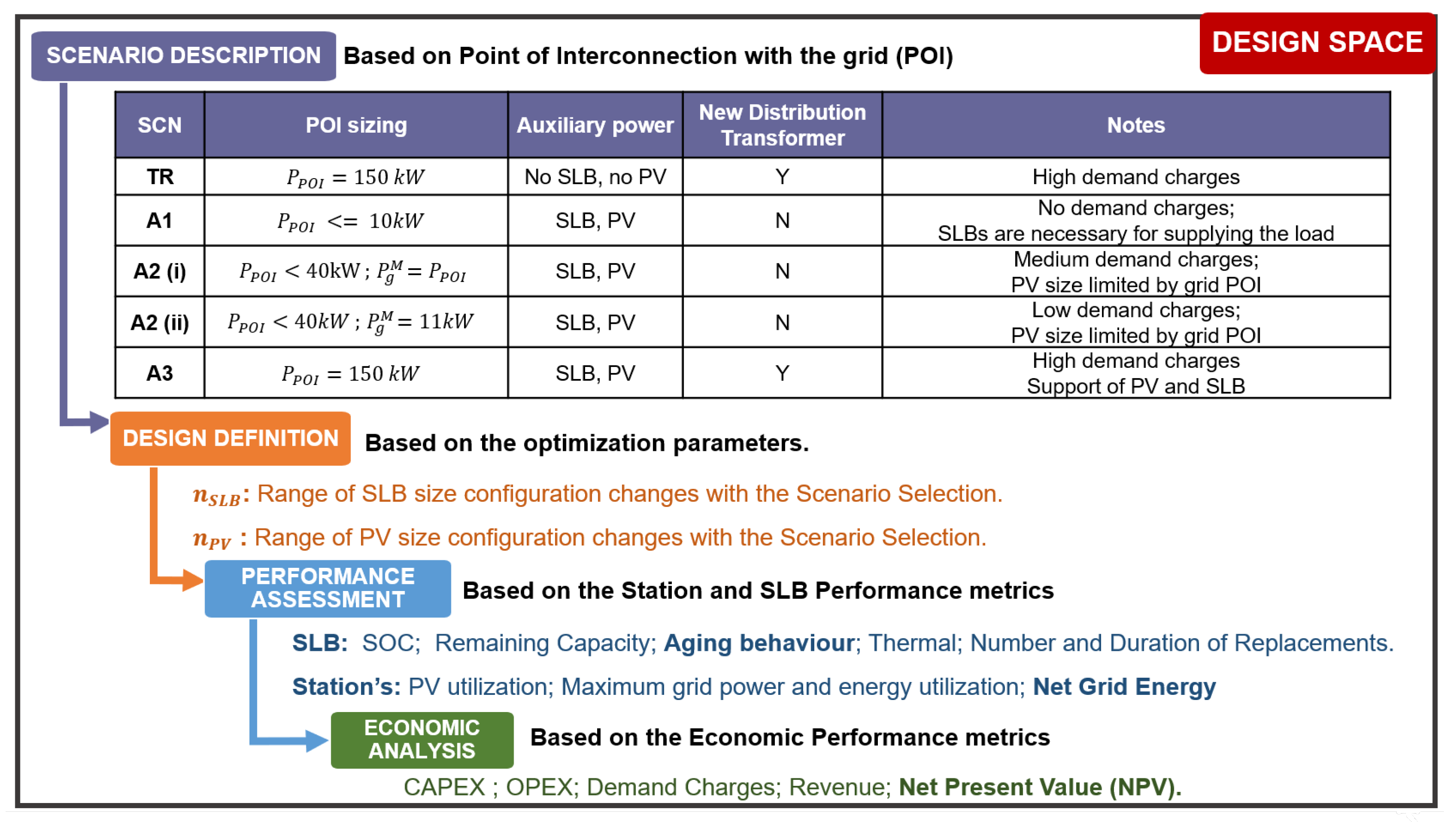
3. Design Space Exploration

A design space exploration problem is solved using an exhaustive search method, with the aim of optimally meeting the desired design requirements from a space of available sets of design parameters [71]. In this work, the design space is the set of configurations of $n_{SLB}$, $n_{PV}$ and $P_{POI}$, and the goal is to find the optimal configuration that provides the highest economic benefits, in terms of NPV, and the technical benefits, in terms of battery and station performances, discussed later in Section 4. The design space is composed of four layers, as follows:

• The first layer is the selection of power of the POI with the grid $P_{POI}$. This layer is also called the scenario description layer, as it enables the selection of different strategies for the station by connecting it to the grid under power levels defined by $P_{POI}$. The table given in Figure 4 describes the scenarios based on their grid $P_{POI}$ and the requirements of transformers.
• The second layer is the selection of sizes or configurations for the SLB and PV [$n_{SLB}$, $n_{PV}$]. The range of sizes of these components is based on the $P_{POI}$ defined in the top layer. One of the major relations the $n_{PV}$ has is that its size is dependent on the size of $P_{POI}$, and the $P_{PV}$ cannot be larger than $P_{POI}$. The details are given in [51], which enables us to form the range of the design parameters of the second layer of the design space based on the first layer.
• The performance modeling layer represents the third layer of the proposed solution, where the selected design parameter configurations from the first and second layers are used as inputs to model the system’s performance. This layer outputs the system-level performance in terms of power, energy, second-life battery aging and other technical characteristics.
• The economic assessment is the final layer. The first and second layers’ design configurations are used to create the CAPEX requirements. It uses inputs from the third layer for power, energy and aging parameters in order to model OPEX and revenue. The main output is the station’s NPV for the selected $P_{POI}$ from the first layer and selected [ $n_{SLB}$, $n_{PV}$] from the second layer. Other performance metrics were also considered, including return on investment (ROI), yearly returns and internal rate of returns. As the electricity tariff is dependent on the $P_{POI}$ [51], the selection of scenario or the point of interconnection to the grid in the first layer plays an important part in the overall system performance.

The design space layers based on the defined scenarios, parameters selection and performance metrics are explained through the architecture in Figure 4.

For each combination of admissible $P_{POI}$, $n_{SLB}$, $n_{PV}$, the tool performs a techno-economic analysis and then compares the different design strategies considering the NPV and other performance metrics. The selection of $P_{POI}$ is based on the various electricity prices, which change depending on the amount of the grid’s used power/energy and the voltage levels. Allocation of PV sizing and power is performed based on the rules defined in the “Interconnection Rules of Distributed Energy Resources (DER)” notations. These rules are referenced according to AEP Ohio’s electricity tariff scheme [51], but these can vary with different utilities.

In order to define the sizing range of $n_{PV}$, the following mentioned procedures are used to determine the scenario selection and the $P_{POI}$ levels, which relate to the $n_{PV}$ size ranges.

In light of the findings in [28], it was decided that the size range of $n_{SLB}$ would be between four packs and seven packs.

To define the appropriate size range for $n_{PV}$, we followed a series of procedures that determine the relevant scenarios and corresponding $P_{POI}$ levels. The factors defined in each scenario allocate the size ranges for $n_{PV}$ based on the electricity tariffs and the range of $P_{POI}$. The $n_{PV}$ size is maintained to be within the permitted range of $P_{POI}$. According to the findings in [28], it was established that the size range for $n_{SLB}$ should be between four packs and seven packs. This range ensures that the number of SLBs is adequate for optimal performance and aligns with the design requirements outlined in the study.

The explanation of these strategies is given below:

• Traditional DCFC: A conventional DC fast-charging station that charges EVs directly from the grid without assistance from other sources is evaluated in this scenario for its economic value. General Service Primary (GS-P) is chosen as the preferable tariff in the traditional DCFC scenario. This scenario offers a baseline for comparing the solutions created and assessing the benefits of deploying multi-source DCFC stations.
• Scenario A1 strategy: Eliminate the demand charges from the proposed DCFC station by grid load and interconnection power reduction. Non-Demand Metered (GS-1) is chosen in order to eliminate the demand charges; this tariff does contain energy and fixed charges, but there are no demand charges as long as the power is limited to 10 kW.
• Scenario A2 strategy: reduce the overall electricity consumption. The goal in this case is to lower overall electricity use, which could also include demand charges. There are two subclassifications created for this scenario in order to examine the potential for consuming the maximum power from the grid $P_g^M$.

  (a)

  Scenario 2.1: $P_g^M$ is taken as the maximum power possible from the grid based on $P_{POI}$. Given that demand charges are determined by the maximum power drawn from the grid rule, this scenario may result in significant demand costs. However, because there is more power available to utilize, it can aid in the quick charging of EVs and SLBs, depending on the control mechanism employed.

  (b)

  Scenario 2.2: $P_g^M$ is restricted to the least amount of power required from the grid to stay in the GS-S tariff, incurring the demand charges (taken as 11 kW) despite the $P_{POI}$ connection level. This strategy helps to allow high grid and PV connections while restricting the demand charges.

• Scenario A3 strategy: This solution involves adding SLBs and PV systems with minimal changes made to the conventional DCFC stations. By connecting the station to the primary-level voltage range, the use case of the proposed DCFC system can be expanded without altering the grid-level functionality of the existing DCFCs. The solution entails adding the required sources and equipment, such as energy management controllers and additional DCDC converters, for the PV and SLB systems to the station.

Table 9. Power and connection parameters for different scenarios.

Parameters	Traditional DCFC	Scenario A1	Scenario A2.1	Scenario A2.2	Scenario A3
Electricity tariff	(GS-Secondary)	(GS-1)	(GS-Secondary)	(GS-Secondary)	(GS-Primary)
$P_{POI}$ (kW)	≤150	≤10	$10\le P_{POI}\le 40$	$10\le P_{POI}\le 40$	150
$P_{PV}^M$ (kW)	NA	≤10	$10\le P_{PV}^M\le 40$	$10\le P_{PV}^M\le 40$	$0\le P_{PV}^M\le 150$
$P_g^M$ (kW)	≤150	≤10	$10\le P_g^M\le 40$	11	11
Transformer	Used	Not Used	Not Used	Not Used	Used

provides a summary of the electricity tariffs, power levels of interconnection and DERs for different scenarios.

Table 10. Scenario-specific cost parameters.

Cost Variables	Units	Scenario A1	Scenario A2.1	Scenario A2.2	Scenario A3 and Traditional DCFC
$C_{dch}$	USD/kW	0	$14.9·P_g^M$	$14.9·P_g^M$	$14.9·P_g^M$
$C_{ech}$	USD/kWh	$0.105·E_{g,NET}$	$0.065·E_{g,NET}$	$0.065·E_{g,NET}$	$0.08·E_{g,NET}$
$C_{trans}$	USD/kW	0	0	0	$250·P_{POI}$

has the scenario-specific cost components that vary based on the electricity tariff used and the $P_{POI}$.

4. Results

In this design space exploration, different scenarios and energy management strategies are explored with various configurations of $n_{SLB}$, $n_{PV}$ and $POI$. The outputs are assessed in terms of techno-economic factors in order to choose the appropriate set of configurations for each scenario and contrast the advantages of utilizing one type of control over another. In order to select the best configurations for each situation and compare the benefits of using one type of control over another, the outputs are evaluated in terms of the following techno-economic parameters:

• Economic performance: These metrics assess the effects of the design parameters on the economy of the investment:

  (a)

  CAPEX: CAPEX is the total capital investment performed for the project. It is accounted for before the project starts operating and gives a measure of the investment cost required for the selected design parameters.

  (b)

  OPEX: OPEX or operating cost includes all the money paid to operate and maintain the charging station. Due to varying energy output from the PV and grid and the dependence of SLB replacements on their size, different configurations may have different operating costs. So it is a good measure to decide the financial requirements weighing the operating vs. capital costs.

  (c)

  Revenue: The revenue through EV charging is fixed, but different PV and SLB configurations may have additional revenue streams through net metering and SLB refunds at the end of the investment.

  (d)

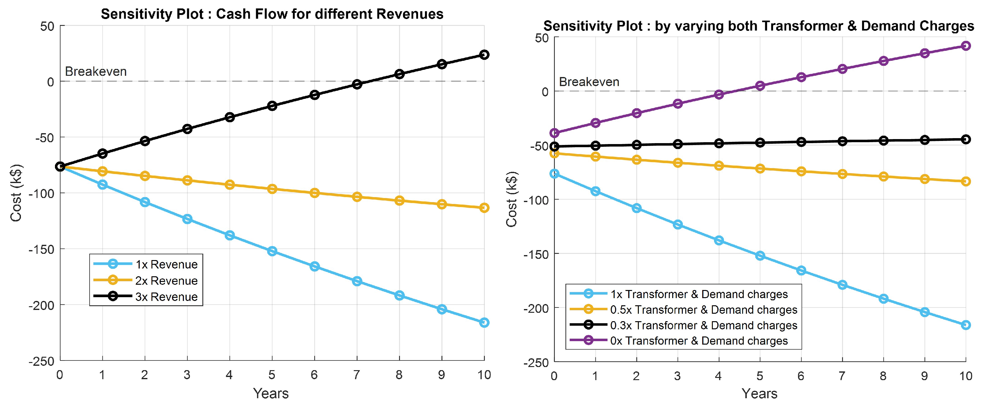
  Demand charge: Higher instantaneous power consumption from the grid results in higher demand charges, which can vary the project goals.

  (e)

  Energy charges: Higher energy consumption from the grid causes higher energy charges, and by increasing the PV sizing, energy consumption can reduce.

  (f)

  Net present value: This is the final economic comparison tool that provides an indication of the value of the project after its completion and involves all the related costs discussed in Section 2.2. The higher the NPV, the higher the financial value of the project, and a negative NPV signifies that the project is not profitable at the end of its life.

• Station performance: This metric assesses the effects of the design parameters and control action on the charging station itself. It allows the project deployment to consider the performance in terms of energy usability and load on the grid.

  (a)

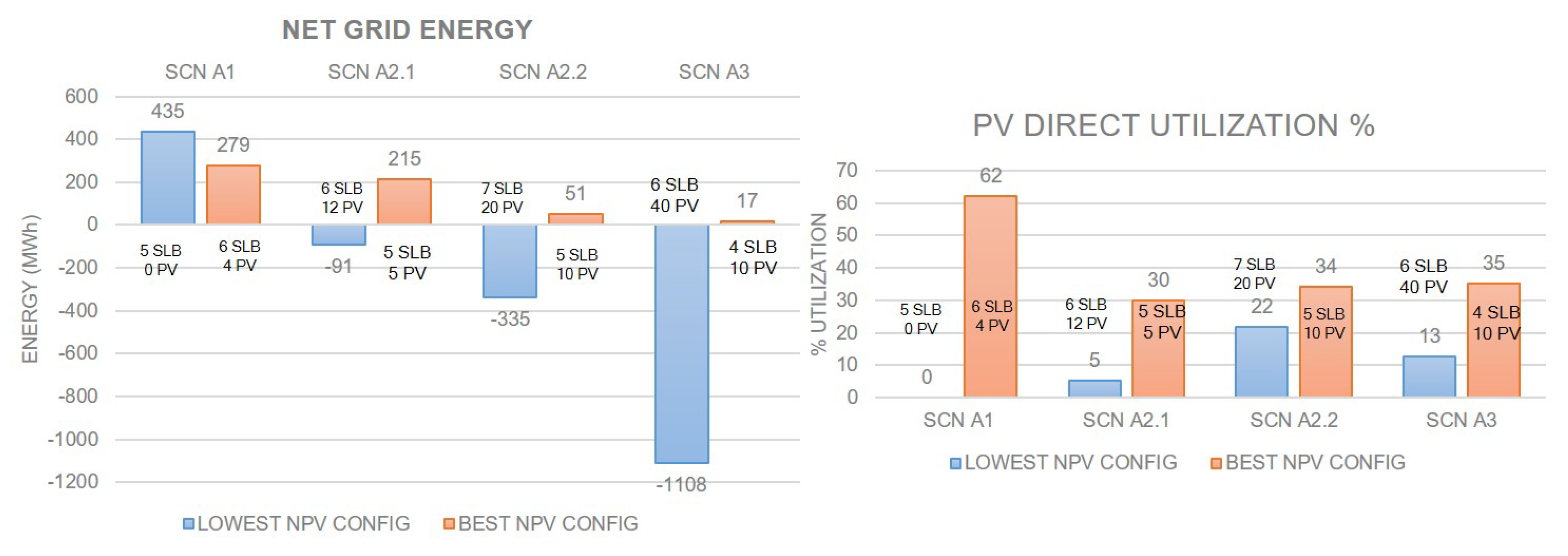
  Net grid energy: This metric is the difference of total grid energy used in a month with the energy supplied back to the grid from PV through net metering [43]. The negative net grid energy is the extra PV energy that could be used in earning solar credits. The less the net energy is, the less the grid energy consumption and the lower the electricity bill.

  $$E_{g,NET}=E_g^{total}-\left(E_{PV}^{total}-E_{PV}^{used}\right)$$

  (10)

  (b)

  Direct PV power utilization: The higher the direct PV utilization, the more suitable it is, as in some locations net metering is not available, and in Ohio net metering is only permitted up to 120% of the total monthly grid energy used. Direct PV utilization is the use of its energy to match the station’s self-consumption. It is crucial to assess which control and configuration strategies are effective because the extra energy created might not be utilized efficiently. The percentage of used PV energy over all available PV energy is used to compute utilization.

  $$E_{PV}^{util}={\displaystyle \frac{E_{PV}^{used}}{E_{PV}^{total}}}$$

  (11)

  (c)

  Maximum power load on the grid: The other aspect of this project is to reduce the load on the grid, and this metric helps in determining the maximum power used from the grid as follows. It is given as $P_g^M$.

• SLB performance: These metrics evaluate the performance of the SLBs for each configuration and scenario. Due to the interdependence of multiple sources, the current, power and energy vary the usage of the battery in the station, resulting in different aging, electrical and thermal characteristics of the SLBs.

  (a)

  State of charge (SOC): The SOC estimate provides the status of batteries and has to be maintained within defined limits during operation. A higher SOC, though, has the benefits of charge available for loads, but keeping SOC too high or low increases the rate of calendar aging [42]. As a function of current and capacity, and relating to the battery’s electrical performance, it gives a good depiction with which to contrast different configurations and scenarios.

  (b)

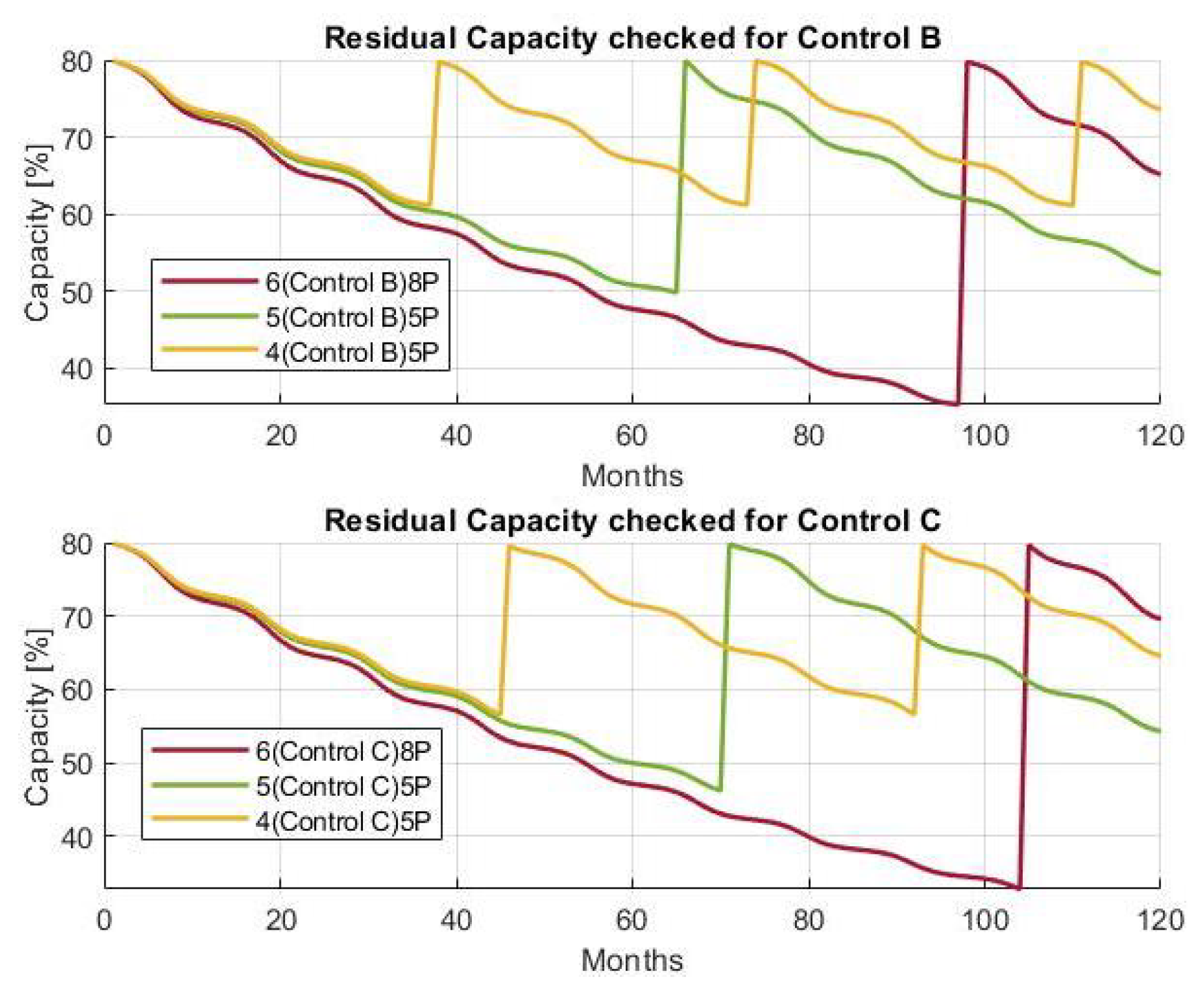
  Remaining capacity and increase in internal resistance: These metrics give an indication of the state-of-health estimation in terms of the energy and capacity deterioration that combines all the calendar and cyclic aging characteristics [42]. The remaining capacity is an indication of how much the battery’s actual capacity is remaining out of the total capacity it has before replacement. The more the battery has been used, the less the remaining capacity it has. The internal resistance, on the other hand, increases with aging and causes power reduction. These both have different effects in terms of battery utilization and replacements for different configurations and are evaluated in the results. The remaining capacity is a metric that indicates the state of health (SoH) of a battery, which takes into account both calendar and cyclic aging characteristics that lead to energy and capacity deterioration. As the battery is used over time, its remaining capacity decreases, reflecting the amount of actual capacity remaining compared to the battery’s original total capacity. Additionally, internal resistance increases with aging, which can cause a reduction in power. These factors have different effects on battery utilization and replacement for different configurations, and are evaluated in the results.

  (c)

  Number of SLB replacements and battery life: The other important factor for deploying the charging station is to understand how quickly and when the SLBs need replacement. Furthermore, this can help in predicting future decisions on the usage and economic investments.

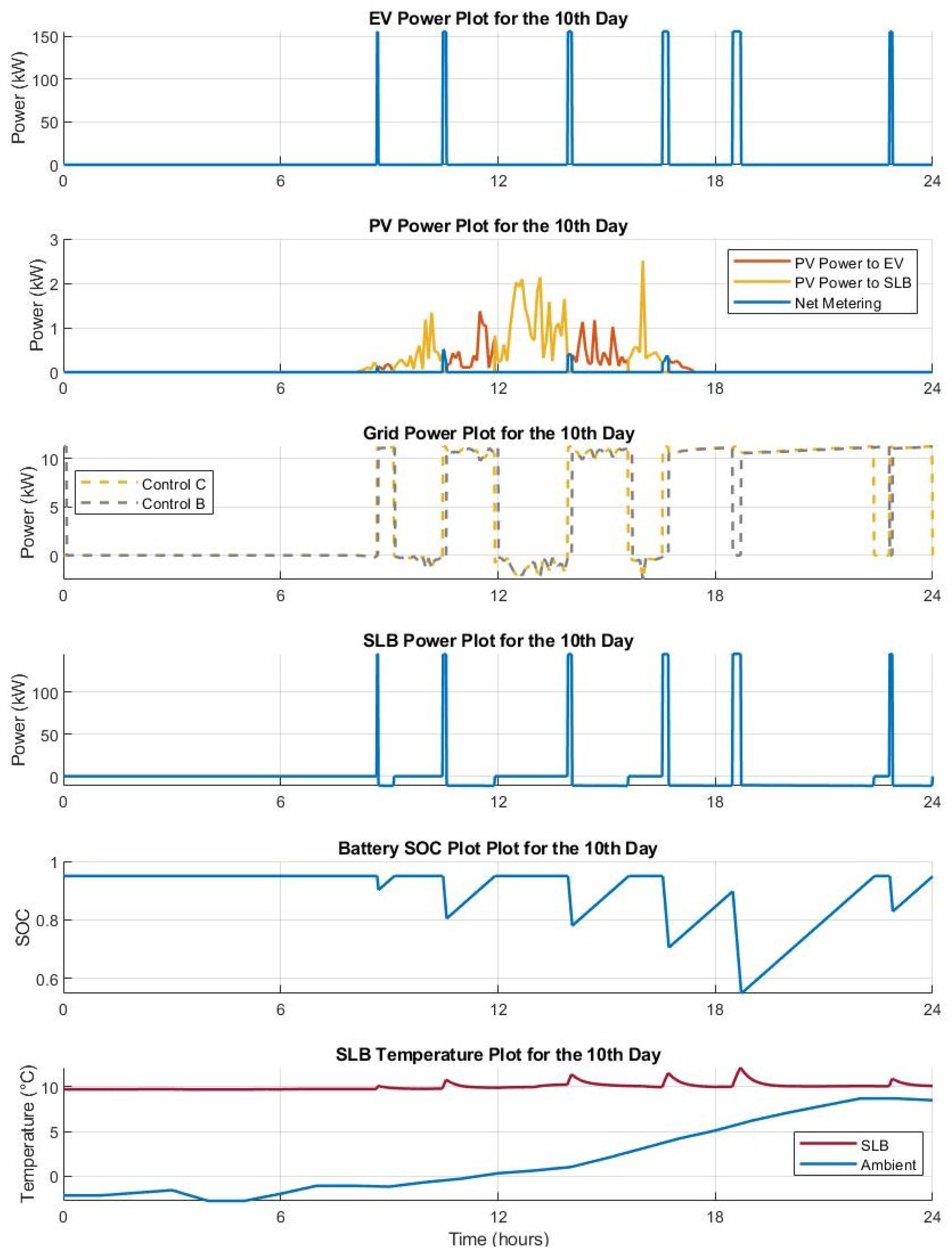
4.1. Selection of Controls

This section focuses on the results of scenario A2.1 to illustrate the impact of various controls and the SLB’s performance for selected configurations. Although multiple scenarios and configurations were analyzed, we present only scenario A2.1 for clarity. While Control A for A2.1 is not detailed here, comparable studies were conducted. Ultimately, Control C was chosen as the primary control for scenarios A2.1, A2.2 and A3 based on technical and budgetary considerations. Control B is recommended for scenario A1.

In Figure 5 and Figure 6, the selected configuration is taken as $n_{PV}$ = 5 and $n_{SLB}$ as 5, and the daily EV energy requirement is 110 kWh. The electrical characteristics of the station and SLB are presented for Controls B and C. The 10th day of a year (10 January) and 150th day (30 May) are plotted against time in hours on the x-axis. The 0th hour represents the start of the day, and the day progresses until the end of 23rd hour (before the 24th hour starts) in the graph. These two days feature a typical winter day when PV power ($P_{PV}$) is minimal and a summer day with high PV power availability. Control B charges the EV using SLB and PV power, whereas Control C charges an EV using SLB, PV and grid power. During the winter season, due to lower PV power availability, both the controls charge an EV utilizing maximum power from the SLB. In Control C, the grid supports the SLB by providing the maximum power possible ($P_g^M$), contrary to Control B when there is no grid support.

During summer, both control strategies B and C can utilize more PV energy to charge EVs. However, the control strategy of C always requires the grid to supply power to EVs, resulting in a high maximum grid power consumption ($P_g^M$). In contrast, control strategy B does not rely on the grid for EV charging, resulting in zero maximum grid power consumption during EV charging. The SLB discharge power has a lower value of roughly 10 kW in Control C as compared to Control B (not displayed in the graphs due to the plot’s visible region restriction). This is due to grid support for EV charging, which reduces the discharges of SLBs and keeps the SOC higher in Control C. When the SLBs are charged, both in Control C and Control B, the PV provides most of the SLB charging power with some support from the grid, keeping the ($P_g^M$) low for both the controls. The unused PV energy is supplied back to the grid in negative value.

As a result, Control B uses less grid power while charging EVs and increases SLB energy and power during EV charging, while Control C uses more grid power during charging EVs but decreases power and energy from SLBs.

In Figure 7 and Figure 8, three different configurations, namely, $n_{SLB}$ = 4, $n_{PV}$ = 5; $n_{SLB}$ = 5, $n_{PV}$ = 5; and $n_{SLB}$ = 6, $n_{PV}$ = 8, are presented for Controls B and C. The analysis reports the results over 10 years of operation of the SLB in the different DCFC station designs. Figure 8 is the plot of the remaining capacity of the SLB ($Q_{SLB}$), plotted against time in months. In both the controls and plots, the configurations with more SLBs have discontinuity, implying a lower number of replacements of SLBs required. As in configuration $n_{SLB}$= 4, $n_{PV}$ = 5, the number of replacements is two, and these are performed around the 37th and 75th month, while in the higher configurations, the replacement time shifts to later months, meaning SLBs need to be replaced later. Control B has more recent replacements than Control C according to a comparison of the controls. This is mostly owing to Control B’s increased SLB discharging power, which results in more power fade and capacity reduction with earlier replacements due to its dependence on current. As SLBs need to be replaced sooner for Control B because they approach their SOC limits before using more capacity, Control B also has more capacity left over than Control C.

From the analysis performed in [42], the configurations with higher ($n_{PV}$, $n_{SLB}$) have a higher rate of calendar aging ($k_{cal}$). This is mostly because of the direct relation between SOC and $k_{cal}$. As evident in Figure 7, configuration 5(SLB)5PV has a lower remaining capacity than configuration 4(SLB)5PV for any control configuration. The future effort to create a control to maintain SOC at an optimal range to slow down calendar aging may benefit from this.

In Figure 8, similar evaluations of capacity remaining are performed between controls and configurations. The x axes of these two graphs display the corresponding mean SOC levels for each month. Since Control C has a greater span and range of SOC than Control B does for a given value of ($Q_{SLB}$), it helps in understanding battery aging behavior for different controls and the selection of Control C over Control B.

4.2. Results for All Scenarios

An overall set of findings for each scenario’s performance in terms of the SLB, station and economics over 10 years are reported in this subsection. The preferred configuration was determined by looking at the configurations with the highest NPV values for each scenario while also taking into account how well the station and SLB performed.

First, a traditional DCFC station is considered. The cash flow with sensitivity analysis is displayed in Figure 9, considering the cost parameters described in Table 4. The sensitivity analysis is shown for the traditional DCFC by increasing the revenue through EV charging (1×, 2× or 3× revenue) on the left plot and by decreasing the demand charges along with transformer cost (1×, 0.5× or 0 demand charges and transformer cost) on the right plot. On the right plot, by reducing both the demand charges and transformer to 0, there is positive cash flow in the system, and NPV is positive at the end of the station cycle. As can be seen, either the income stream needs to be increased threefold or the transformer and demand charges need to be reduced in order to have a positive NPV. For the baseline values, the cash flow is negative due to the high cost of the transformer and the demand charges. The break-even cost, which indicates the year the project has paid for itself in full, is achievable in the seventh year of operation by increasing the income stream to three times or in the fourth year by removing the demand charges and the cost of the transformer.

For the proposed DCFC station, design space for all the scenarios with their possible ranges of configurations is evaluated and shown in Figure 10 as a grid with 3D bars. NPV values are plotted on the y axis, the SLB configurations on the x axis and the PV configurations on the z axis; these are all represented as 3D bars in Figure 10. The four scenarios are shown on the same graph along with the selected control strategies for all scenarios, A1, A2.1, A2.2 and A3. For example, scenario A1 is under Control B, while scenarios A2.1, A2.2 and A3 are under Control C. The configurations with the highest NPV for all scenarios are selected as the preferred configurations. The economic indicators in terms of NPV and OPEX are provided in Figure 11 for the configurations providing the highest NPV values. The cash-flow plot shows that all of the scenarios begin to generate income and reach positive cash flow after about seven years. Although scenario A3’s configuration 4($n_{SLB}$) with 10($n_{PV}$) has a negative end NPV, the trend is moving in the direction of positive or zero cash flow, indicating that there may eventually be some positive cash flow over a longer period of operation, which is different from what is seen for traditional DCFC stations in Figure 9.

The plots in Figure 12 for each of the scenarios with the highest NPV provide a full breakdown of costs in CAPEX, OPEX and revenue in the left plot, with the breakdown of OPEX expenditures in the right plot. The NPV of scenario A3 is negative since it has more CAPEX and OPEX than revenue. The CAPEX is always the biggest expense, and the OPEX varies depending on its components. There are no demand charges in scenario A1, and energy costs account for the majority of OPEX. In A2.2, there is a marginally lower demand charge than in A2.1 but a significant reduction in energy charges due to the addition of more PV strings; while this does increase A2.2 CAPEX costs, they are offset by a decrease in overall OPEX. Due to similar grid power usage and PV size as A2.2, A3 has comparable demand charges and energy charges but more battery replacements due to its smaller battery size.

Figure 13 shows that the right plot represents the amount of PV energy used for self-consumption through EV and SLB charging, while the left plot represents the net grid energy consumed. The availability of PV energy means that scenario A1 with four PVs uses less grid energy than scenario A1 without PVs. The orange bar shows the configuration of PVs and SLBs with the highest NPV values, while the blue bars represent those with the lowest NPV values.

However, due to high PV sizes, there is negative net energy that is given to the grid in all other situations from the lower NPV setups. The right plot shows that the orange bars have better PV direct usage than blue ones due to effective PV scaling. The excess 20% of energy can be sold to the grid through solar renewable credits, in addition to the 100% utilization to match the station’s energy demand. Therefore, up to 120 percent of the generated energy may be useful. However, having greater PV sizes than necessary is inefficient and cannot be sold beyond 120 percent.

Table 11. Summary of economics and grid load reduction for the highest NPV configurations selected for each scenario. The summary table shows the maximum power used from grid, capital cost, NPV and % change in NPV and grid load for the selected configurations.

Scenario	Max Grid Power Used	Selected Configuration	Grid Load Shedding	Installment Cost	Highest NPV	NPV Increase %
Traditional DCFC	150 kW	N/A	0%	USD 76,700	USD −216,138	N/A
A1—secondary electricity tariff without demand charges	10 kW	$n_{SLB}=6$  $n_{PV}=4$	93%	USD 49,800	USD 25,100	111%
A2(i)—secondary electricity tariff with demand charges	12 kW	$n_{SLB}=5$  $n_{PV}=5$	92%	USD 51,900	USD 21,875	110%
A2(ii)—secondary electricity tariff with demand charges	11 kW	$n_{SLB}=5$  $n_{PV}=10$	92.6%	USD 59,600	USD 24,447	111%
A3—primary electricity tariff with demand charges	11 kW	$n_{SLB}=2$  $n_{PV}=10$	92.6%	USD 128,800	USD −48,810	78%

provides a summary for the selected configurations with the highest NPV values for all the scenarios along with the traditional DCFC. The table summarizes the monetary value and grid load reduction each configuration has along with the installment capital required. The selected configurations in terms of sizes $n_{PV}$ and $n_{SLB}$ are given for each scenario.

5. Conclusions

Traditional DCFC stations are impacting the grid with uncoordinated and high power load demand. According to the present trends in station utilization and EV adoption, DCFC stations require significant capital investments and, in this research, are found to not be profitable.

Through the development of a DCFC station with integrated second-life batteries (SLBs) and a PV system, the techno-economic variables in terms of NPV, station performance and battery performance were maximized. A model was developed to study the DCFC station behavior using event-based EV load profiles, real PV data inputs, experimentally calibrated electrical, aging and thermal properties of the batteries and efficiency maps for power transfer. To ensure the energy management controller capability to maximize the performance of the station, many control strategies were analyzed. A design space with several scenarios depending on the power level of the point of interconnection to the grid, including voltage ranges, power ranges and transformer use cases, was built to help choose the sizing of batteries and PVs. The financial model was calibrated considering realistic electricity costs. The electrical standards of AEP Ohio were adhered to, and parameters were calibrated using a large data set from national labs, industry and academic research to keep the scenarios appropriate for real-life applications. Performance measures that aid in comprehending the trends of economics, station operation and battery aging for various configurations were developed in order to examine the data and choose the best configuration for each scenario. The analysis considered a 10-year time frame. A conventional DCFC station was also used to compared the impact of the selected technologies.

From this paper, there are the following leanings and observations made:

• Traditional DCFC stations for 150 kW are not economically convenient over 10 years of usage.
• Even with the cost of the transformer removed, revenues increased or power costs decreased, the standard DCFC can only just match the investment cost.
• If properly designed and managed, a DCFC with integrated storage and renewable resources can reduce grid demand while still providing a favorable return on investment.
• This work examined various methods for visualizing and presenting DCFC station and ESS parameters, which show how the charging station and ESS operate.
• This aids in choosing different configurations, as needed, based on different parameters, such as the maximum SOC retention or the lowest SLB replacement duration.
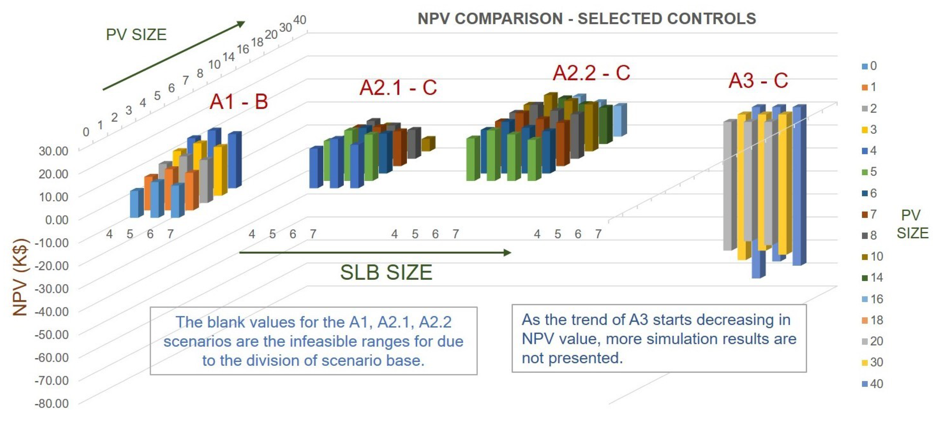
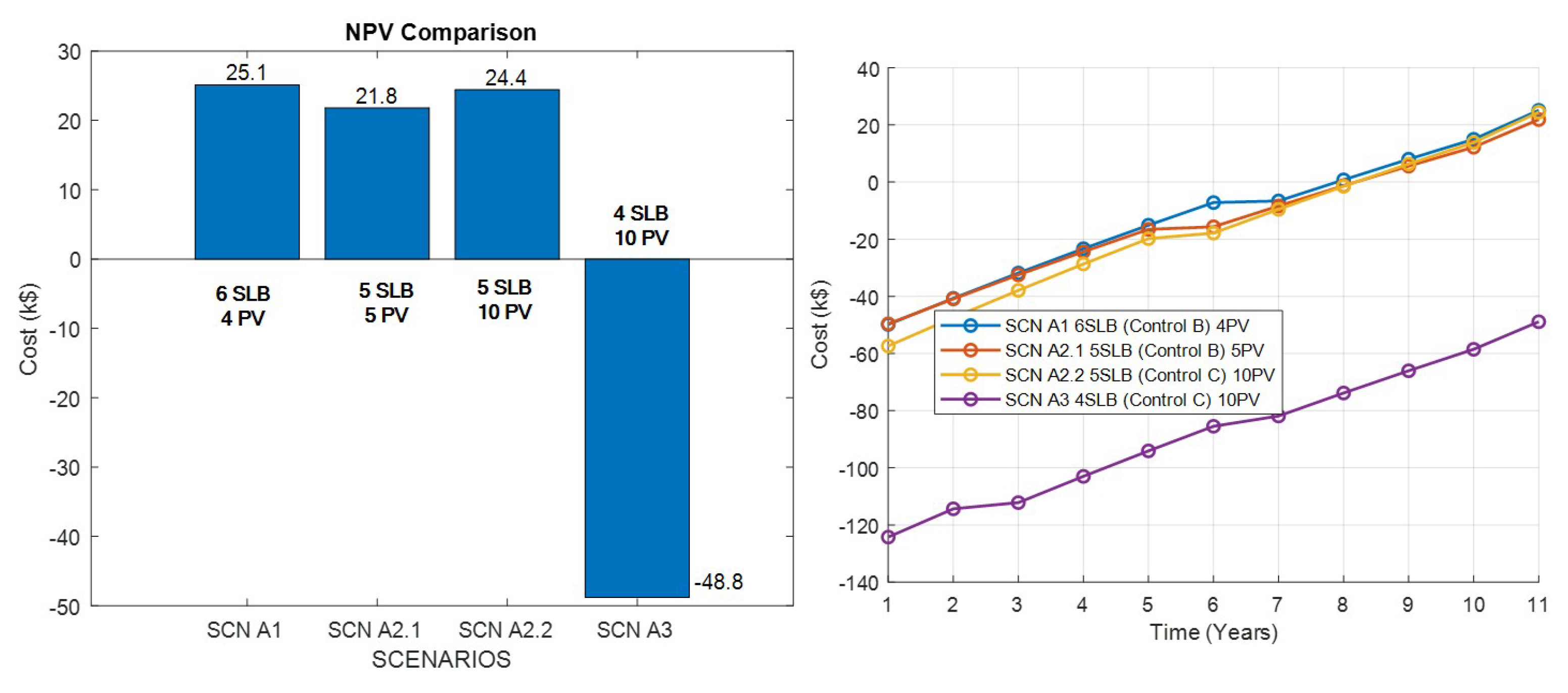
• For all the scenarios used, the proposed DCFC station architecture has better NPV results with the optimally selected size of SLB packs and PV strings.
• The scenarios A1, A2.1 and A2.2 show high NPV profits with the optimized configurations of PVs and SLBs.
• The scenarios A1, A2.1 and A2.2 have reduced installment cost (CAPEX).
• Despite having a lower NPV than the conventional DCFC, scenario A3 still outperforms it in terms of NPV value and grid load utilization. Nevertheless, when batteries and PV systems are added to the 150 kW DCFC with high power interconnection, it has the most expensive installation costs due to interconnection cost added to the DERs cost.
• It can be postulated that in terms of maximum power required by the DCFC station from the grid, there is a significant reduction in every scenario.

References

1. Rafi, M.A.H.; Bauman, J. A comprehensive review of DC fast-charging stations with energy storage: Architectures, power converters, and analysis. IEEE Trans. Transp. Electrif. 2020, 7, 345–368. [Google Scholar] [CrossRef]
2. Deb, N.; Singh, R.; Brooks, R.R.; Bai, K. A Review of Extremely Fast Charging Stations for Electric Vehicles. Energies 2021, 14, 7566. [Google Scholar] [CrossRef]
3. Amry, Y.; Elbouchikhi, E.; Le Gall, F.; Ghogho, M.; El Hani, S. Electric Vehicle Traction Drives and Charging Station Power Electronics: Current Status and Challenges. Energies 2022, 15, 6037. [Google Scholar] [CrossRef]
4. Wang, L.; Qin, Z.; Slangen, T.; Bauer, P.; Van Wijk, T. Grid impact of electric vehicle fast charging stations: Trends, standards, issues and mitigation measures-an overview. IEEE Open J. Power Electron. 2021, 2, 56–74. [Google Scholar] [CrossRef]
5. Mahfouz, M.M.; Iravani, M.R. Grid-integration of battery-enabled dc fast charging station for electric vehicles. IEEE Trans. Energy Convers. 2019, 35, 375–385. [Google Scholar] [CrossRef]
6. Anwar, M.B.; Muratori, M.; Jadun, P.; Hale, E.; Bush, B.; Denholm, P.; Ma, O.; Podkaminer, K. Assessing the value of electric vehicle managed charging: A review of methodologies and results. Energy Environ. Sci. 2022, 15, 466–498. [Google Scholar] [CrossRef]
7. Habib, S.; Khan, M.M.; Abbas, F.; Sang, L.; Shahid, M.U.; Tang, H. A comprehensive study of implemented international standards, technical challenges, impacts and prospects for electric vehicles. IEEE Access 2018, 6, 13866–13890. [Google Scholar] [CrossRef]
8. Hamadi, A.; Arefifar, S.A.; Alam, M.S. EV Battery Charger Impacts on Power Distribution Transformers Due to Harmonics; SAE Technical Paper. 2022. Available online: https://www.sae.org/publications/technical-papers/content/2022-01-0750/ (accessed on 30 May 2022).
9. Hoehne, C.; Muratori, M.; Jadun, P.; Bush, B.; Yip, A.; Ledna, C.; Vimmerstedt, L.; Podkaminer, K.; Ma, O. Exploring decarbonization pathways for USA passenger and freight mobility. Nat. Commun. 2023, 14, 6913. [Google Scholar] [CrossRef]
10. Pacific Gas & Electric. Electric Program Investment Charge (EPIC). Available online: https://www.pge.com (accessed on 30 May 2022).
11. Nicholas, M.; Hall, D. Lessons Learned on Early Electric Vehicle Fast-Charging Deployments; International Council on Clean Transportation: Washington, DC, USA, 2018; pp. 7–26. [Google Scholar]
12. Nelder, C.; Rogers, E. Reducing EV Charging Infrastructure Costs; Rocky Mountain Institute: Basalt, CO, USA, 2019. [Google Scholar]
13. Eckerle, T.; Vacin, G.B. Electric Vehicle Charging Station Permitting Guidebook. Available online: https://businessportal.ca.gov (accessed on 29 October 2022).
14. Alternative Fuels Data Center. Driving into 2025: The Future of Electric Vehicles. Available online: https://afdc.energy.gov (accessed on 30 May 2022).
15. Monkman, R. EV Charging Infrastructure: Understanding Your City’s Building Code Requirements. Available online: https://www.chargeup-usa.com (accessed on 29 October 2022).
16. Gjelaj, M.; Træholt, C.; Hashemi, S.; Andersen, P.B. Optimal Design of DC Fast-Charging Stations for EVs in Low Voltage Grids. In Proceedings of the 2017 IEEE Transportation Electrification Conference and Expo (ITEC), Pune, India, 13–15 December 2017; pp. 684–689. [Google Scholar]
17. Bai, S.; Yu, D.; Lukic, S. Optimum Design of an EV/PHEV Charging Station with DC Bus and Storage System. In Proceedings of the 2010 IEEE Energy Conversion Congress and Exposition, Atlanta, GA, USA, 12–16 September 2010; pp. 1178–1184. [Google Scholar]
18. Leone, C.; Longo, M. Modular approach to ultra-fast charging stations. J. Electr. Eng. Technol. 2021, 16, 1971–1984. [Google Scholar] [CrossRef]
19. O’Connor, P.; Jacobs, M. Charging Smart: Drivers and Utilities Can both Benefit from Well-Integrated Electric Vehicles and Clean Energy. 2017. Available online: https://trid.trb.org/View/1470898 (accessed on 30 June 2022).
20. Kandil, S.M.; Farag, H.E.; Shaaban, M.F.; El-Sharafy, M.Z. A combined resource allocation framework for PEVs charging stations, renewable energy resources and distributed energy storage systems. Energy 2018, 143, 961–972. [Google Scholar] [CrossRef]
21. Sa’adati, R.; Jafari-Nokandi, M.; Saebi, J. Allocation of RESs and PEV fast-charging station on coupled transportation and distribution networks. Sustain. Cities Soc. 2021, 65, 102527. [Google Scholar] [CrossRef]
22. Pal, A.; Bhattacharya, A.; Chakraborty, A.K. Placement of public fast-charging station and solar distributed generation with battery energy storage in distribution network considering uncertainties and traffic congestion. J. Energy Storage 2021, 41, 102939. [Google Scholar] [CrossRef]
23. Borlaug, B.; Bennett, J. EV Charging and the Impacts of Electricity Demand Charges; Technical Report; National Renewable Energy Lab. (NREL): Golden, CO, USA, 2022. [Google Scholar]
24. Freewire: Boost Charger Freewire. Available online: https://freewiretech.com (accessed on 29 October 2022).
25. Powerstar: Battery Buffered EV Charging. Available online: https://powerstar.com (accessed on 29 October 2022).
26. GenZ EV Solutions: GenZ EV Solutions Enters the U.S. EV Battery-Buffered, Ultra-Fast Charger Market. Available online: https://www.prnewswire.com (accessed on 29 October 2022).
27. Kamath, D.; Shukla, S.; Arsenault, R.; Kim, H.C.; Anctil, A. Evaluating the cost and carbon footprint of second-life electric vehicle batteries in residential and utility-level applications. Waste Manag. 2020, 113, 497–507. [Google Scholar] [CrossRef] [PubMed]
28. D’Arpino, M.; Cancian, M. Design of a Grid-Friendly dc Fast Charge Station with Second Life Batteries; Technical Report, SAE Technical Paper. 2019. Available online: https://www.sae.org/publications/technical-papers/content/2019-01-0867/ (accessed on 30 June 2023).
29. Gao, Y.; Cai, Y.; Liu, C. Annual operating characteristics analysis of photovoltaic-energy storage microgrid based on retired lithium iron phosphate batteries. J. Energy Storage 2022, 45, 103769. [Google Scholar] [CrossRef]
30. Leone, C.; Peretti, C.; Paris, A.; Longo, M. Photovoltaic and battery systems sizing optimization for ultra-fast charging station integration. J. Energy Storage 2022, 52, 104995. [Google Scholar] [CrossRef]
31. Gjelaj, M.; Træholt, C.; Hashemi, S.; Andersen, P.B. Cost-benefit analysis of a novel DC fast-charging station with a local battery storage for EVs. In Proceedings of the 2017 52nd International Universities Power Engineering Conference (UPEC), Heraklion, Crete, Greece, 28–31 August 2017; pp. 1–6. [Google Scholar]
32. Yang, L.; Ribberink, H. Investigation of the potential to improve DC fast charging station economics by integrating photovoltaic power generation and/or local battery energy storage system. Energy 2019, 167, 246–259. [Google Scholar] [CrossRef]
33. Elibol, B.; Poyrazoglu, G.; Çalışkan, B.C.; Kaya, H.; Armağan, Ç.; Akınç, H.E.; Kaymaz, A. Battery Integrated Off-grid DC Fast Charging: Optimised System Design Case for California. In Proceedings of the 2021 10th International Conference on Renewable Energy Research and Application (ICRERA), Istanbul, Turkey, 26–29 September 2021; pp. 327–332. [Google Scholar]
34. Bhatti, A.R.; Salam, Z.; Sultana, B.; Rasheed, N.; Awan, A.B.; Sultana, U.; Younas, M. Optimized sizing of photovoltaic grid-connected electric vehicle charging system using particle swarm optimization. Int. J. Energy Res. 2019, 43, 500–522. [Google Scholar] [CrossRef]
35. Muratori, M.; Elgqvist, E.; Cutler, D.; Eichman, J.; Salisbury, S.; Fuller, Z.; Smart, J. Technology solutions to mitigate electricity cost for electric vehicle DC fast charging. Appl. Energy 2019, 242, 415–423. [Google Scholar] [CrossRef]
36. Muratori, M.; Kontou, E.; Eichman, J. Electricity rates for electric vehicle direct current fast charging in the United States. Renew. Sustain. Energy Rev. 2019, 113, 109235. [Google Scholar] [CrossRef]
37. Edge, J.S.; O’Kane, S.; Prosser, R.; Kirkaldy, N.D.; Patel, A.N.; Hales, A.; Ghosh, A.; Ai, W.; Chen, J.; Yang, J.; et al. Lithium ion battery degradation: What you need to know. Phys. Chem. Chem. Phys. 2021, 23, 8200–8221. [Google Scholar] [CrossRef]
38. Baghdadi, I.; Briat, O.; Delétage, J.Y.; Gyan, P.; Vinassa, J.M. Lithium battery aging model based on Dakin’s degradation approach. J. Power Sources 2016, 325, 273–285. [Google Scholar] [CrossRef]
39. Liu, G.; Chinthavali, M.S.; Debnath, S.; Tomsovic, K. Optimal m Sizing of an Electric Vehicle Charging Station with Integration of PV and Energy Storage. In Proceedings of the 2021 IEEE Power & Energy Society Innovative Smart Grid Technologies Conference (ISGT), Washington, DC, USA, 16–18 February 2021; pp. 1–5. [Google Scholar]
40. Domínguez-Navarro, J.; Dufo-López, R.; Yusta-Loyo, J.; Artal-Sevil, J.; Bernal-Agustín, J. Design of an electric vehicle fast-charging station with integration of renewable energy and storage systems. Int. J. Electr. Power Energy Syst. 2019, 105, 46–58. [Google Scholar] [CrossRef]
41. D’Arpino, M.; Singh, G.; Koh, M.B. Impact of Event-Based EV Charging Power Profile on Design and Control of Multi-Source DCFC Stations; Technical Report, SAE Technical Paper. 2023. Available online: https://www.sae.org/publications/technical-papers/content/2023-01-0706/ (accessed on 30 June 2023).
42. D’Arpino, M.; Cancian, M. Lifetime optimization for a grid-friendly dc fast charge station with second life batteries. ASME Lett. Dyn. Syst. Control 2021, 1, 011014. [Google Scholar] [CrossRef]
43. PUCO. Public Utility Commission of Ohio. PUCO Rule 4901:1-10-28|Net Metering. Available online: https://codes.ohio.gov/ohio-administrative-code/rule-4901:1-10-28 (accessed on 30 June 2023).
44. Singh, G. Development and Sizing of the multi-source DC Fast Charging Station using Second Life Batteries and Renewables. Master’s Thesis, The Ohio State University, Columbus, OH, USA, 2022. [Google Scholar]
45. Ganesh, S.V.; D’Arpino, M. Critical Comparison of Li-Ion Aging Models for Second Life Battery Applications. Energies 2023, 16, 3023. [Google Scholar] [CrossRef]
46. D’Arpino, M.; Regmi, N.; Ketineni, P. Impact of battery pack power limits on vehicle performance. In Proceedings of the 2023 IEEE Transportation Electrification Conference & Expo (ITEC), Chiang Mai, Thailand, 28 November–1 December 2023; pp. 1–8. [Google Scholar]
47. National Renewable Energy Laboratory. Solar Resource Maps and Data. Available online: https://www.nrel.gov/gis/solar-resource-maps.html (accessed on 30 May 2022).
48. BP Solar. BP 3235T 235 Watt 29 Volt Solar Panel. Available online: https://www.ecodirect.com (accessed on 30 May 2022).
49. De Soto, W.; Klein, S.A.; Beckman, W.A. Improvement and validation of a model for photovoltaic array performance. Sol. Energy 2006, 80, 78–88. [Google Scholar] [CrossRef]
50. De Brito, M.A.G.; Galotto, L.; Sampaio, L.P.; e Melo, G.d.A.; Canesin, C.A. Evaluation of the main MPPT techniques for photovoltaic applications. IEEE Trans. Ind. Electron. 2012, 60, 1156–1167. [Google Scholar] [CrossRef]
51. American Electric Power. PUCO Rules. February 2022. Available online: https://www.aepohio.com/company/about/rates/ (accessed on 30 June 2023).
52. Flett Exchange. Spot Data for Ohio SREC Market. Available online: https://www.flettexchange.com (accessed on 30 May 2022).
53. SREC Trade: SREC OHIO. Available online: https://www.srectrade.com/markets/rps/srec/ohio (accessed on 30 May 2022).
54. Mongird, K.; Viswanathan, V.; Alam, J.; Vartanian, C.; Sprenkle, V. Energy Storage Grand Challenge Cost and Performance Assessment 2020; Technical Report; Pacific Northwest National Laboratory, US Department of Energy: Richland, WA, USA, 2020.
55. Mongird, K.; Viswanathan, V.V.; Balducci, P.J.; Alam, M.J.E.; Fotedar, V.; Koritarov, V.S.; Hadjerioua, B. Energy Storage Technology and Cost Characterization Report; Technical Report; Pacific Northwest National Lab. (PNNL): Richland, WA, USA, 2019.
56. Feldman, D.; Ramasamy, V.; Fu, R.; Ramdas, A.; Desai, J.; Margolis, R. US Solar Photovoltaic System and Energy Storage Cost Benchmark (Q1 2020); Technical Report; National Renewable Energy Lab. (NREL): Golden, CO, USA, 2021.
57. Vimmerstedt, L.J.; Akar, S.; Augustine, C.R.; Beiter, P.C.; Cole, W.J.; Feldman, D.J.; Kurup, P.; Lantz, E.J.; Margolis, R.M.; Stehly, T.J.; et al. 2019 Annual Technology Baseline; Technical Report; National Renewable Energy Lab. (NREL): Golden, CO, USA, 2019.
58. Kim, D.K.; Yoneoka, S.; Banatwala, A.Z.; Kim, Y.T.; Nam, K. Handbook on Battery Energy Storage System; Asian Development Bank: Manila, Philippines, 2018. [Google Scholar]
59. Kelleher Environmental; Energy API. Research Study on Reuse and Recycling of Batteries Employed in Electric Vehicles: The Technical, Environmental, Economic, Energy and Cost Implications of Reusing and Recycling EV Batteries. 2019. Available online: https://www.api.org/~/media/files/oil-and-natural-gas/fuels/kelleher%20final%20ev%20battery%20reuse%20and%20recycling%20report%20to%20api%2018sept2019%20edits%2018dec2019.pdf (accessed on 30 May 2022).
60. Foster, M.; Isely, P.; Standridge, C.R.; Hasan, M.M. Feasibility assessment of remanufacturing, repurposing, and recycling of end of vehicle application lithium-ion batteries. J. Ind. Eng. Manag. (JIEM) 2014, 7, 698–715. [Google Scholar] [CrossRef]
61. Rallo, H.; Casals, L.C.; De La Torre, D.; Reinhardt, R.; Marchante, C.; Amante, B. Lithium-ion battery 2nd life used as a stationary energy storage system: Ageing and economic analysis in two real cases. J. Clean. Prod. 2020, 272, 122584. [Google Scholar] [CrossRef]
62. Neubauer, J.; Pesaran, A.; Williams, B.; Ferry, M.; Eyer, J. Techno-Economic Analysis of PEV Battery Second Use: Repurposed-Battery Selling Price and Commercial and Industrial End-User Value; Technical Report; National Renewable Energy Lab. (NREL): Golden, CO, USA, 2012.
63. Cole, W.; Frazier, A.W.; Augustine, C. Cost Projections for Utility-Scale Battery Storage: 2021 Update; Technical Report; National Renewable Energy Lab. (NREL): Golden, CO, USA, 2021.
64. Burnham, A.; Dufek, E.J.; Stephens, T.; Francfort, J.; Michelbacher, C.; Carlson, R.B.; Zhang, J.; Vijayagopal, R.; Dias, F.; Mohanpurkar, M.; et al. Enabling fast charging–Infrastructure and economic considerations. J. Power Sources 2017, 367, 237–249. [Google Scholar] [CrossRef]
65. DCFC Cost Components: Much More than Electricity: Spot Data for Ohio SREC Market. Available online: https://www.evgo.com (accessed on 30 May 2022).
66. Learn How to Easily Upgrade Your EV Charging Installation. Available online: https://freewiretech.com/upgrade-your-ev-charger/ (accessed on 30 May 2022).
67. EVGO. EV Rates—EVgo. Available online: https://www.evgo.com/pricing/ (accessed on 30 May 2022).
68. Livewire. Cost to Charge an EV. Available online: https://www.lifewire.com/cost-to-charge-an-ev-5203305 (accessed on 30 May 2022).
69. Electrify America. Pricing. Available online: https://www.electrifyamerica.com/pricing/ (accessed on 30 May 2022).
70. Investopedia. NPV Calculation. Available online: https://www.investopedia.com/ (accessed on 30 May 2022).
71. Kang, E.; Jackson, E.; Schulte, W. An approach for effective design space exploration. In Proceedings of the Monterey Workshop; Springer: Berlin/Heidelberg, Germany, 2010; pp. 33–54. [Google Scholar]
Figure 1. Architecture of the proposed DCFC system.
Energies 17 04012 g001
Figure 2. Modeling framework for the DCFC station with its subsystems.
Energies 17 04012 g002
Figure 3. Classification of cost components for DCFC station.
Energies 17 04012 g003
Figure 4. Design space exploration architecture.
Energies 17 04012 g004
Figure 5. Analysis for the 10th day of year 1: EV load, PV power, grid power, SLB power, SLB SOC and temperature.
Energies 17 04012 g005
Figure 6. Analysis for the 150th day of year 1: EV load, PV power, grid power, SLB power, SLB SOC and temperature.
Energies 17 04012 g006
Figure 7. Residual capacity vs. time in months for different control architectures—Control B (top plot) and Control C (bottom plot).
Energies 17 04012 g007
Figure 8. Residual capacity vs. mean SOC for different control architectures—Control B (top plot) and Control C (bottom plot).
Energies 17 04012 g008
Figure 9. Sensitivity analysis for traditional DCFC—revenue (left plot) and demand charges and transformer cost (right plot).
Energies 17 04012 g009
Figure 10. NPV results for all scenarios with all configurations and their selected controls.
Energies 17 04012 g010
Figure 11. NPV (left plot) and cash flow (right plot) for the selected configurations with the highest NPV among all scenarios.
Energies 17 04012 g011
Figure 12. Cost breakdown (left plot ) and OPEX cost (right plot) for the selected configurations with the highest NPV among all scenarios.
Energies 17 04012 g012
Figure 13. Net grid energy (left plot ) and PV direct utilization expressed in % (right plot) for the highest and lowest NPV configurations among all scenarios.
Energies 17 04012 g013