Numerical Simulation to Investigate the Effect of Adding a Fixed Blade to a Magnus Wind Turbine

Abstract

The investigation of aerodynamics and the establishment of flow patterns around finite-length cylinders with various end shapes in a free, boundless air flow with longitudinal and transverse flow over a wide range of geometric and regime parameters is sketchy and does not have a wide range of geometric and regime parameters. This, in turn, affects the entire aerodynamics of the streamlined body. This paper considers the numerical simulation of a wind turbine made of combined blades. CFD (computational fluid dynamics) methods based on the realisable k-ε turbulence model were used in the study. The results on the influence of the position of the fixed blade on the angle of inclination are obtained (0°, 15°, 30°, 45°, and 60°). The authors found that the pressure of a fixed blade at an optimal angle increases the power coefficient Cp by 35–40%. The dependence of the Cp power coefficient on the rotational speed (speed coefficient) for a three-bladed wind turbine was also established, and it was determined that the maximum value of Cp = 0.28 at Z = 4.9. Based on the results obtained, it was determined that the wind turbine has a maximum power coefficient at an angle of inclination of 0 degrees.

1. Introduction

Alternative energy sources are environmentally friendly and help preserve the environment. Factors such as rising prices for fossil sources, the phenomenon of global warming, instability of the energy market, and an increase in greenhouse gas emissions contribute to their widespread use [1]. Wind energy is continually advancing on a global scale, becoming a key component in the energy systems of many countries that have made significant investments in this sector [2]. The yearly rise in global wind energy consumption enhances its integration into the energy system and bolsters its contribution to the total energy supply. The total installed wind generation capacity in 2022 amounted to 837 GW worldwide, and 141 billion were invested dollars [3]. It is known that China is in first place in terms of generating energy using wind energy with a capacity of 221 GW, the second place is occupied by the United States with a production capacity of 96.4 GW, and the third place is occupied by Germany with 59.3 GW, becoming the largest consumer of wind energy in Europe.

The basis of the mechanism for generating electrical energy is the conversion of kinetic energy, on which all wind turbines are based. Wind turbines come with horizontal (HAWT) [4,5,6] and vertical (VAWT) axes wind turbines [7,8,9], depending on the location of the blades. In practice, HAWTs are increasingly used [10] due to the reliability of the installation and high output power, which differ in the shape and design of the blades, and these, along with advantages, also have disadvantages [11]. One example is standard wind turbines with wing-shaped blades. The paper [12] presents the results of determining designs of power elements of a HAWT with a capacity of 5 MW using the inverse finite element method (iFEM) under actual loading conditions. It was determined that iFEM is a suitable method for determining the wind turbine blade’s shape. The authors in [13] experimentally investigated the effect of the shape of the leading edge on the performance of the entire wind turbine. Experimental studies were conducted at Reynolds numbers 4.7 × 10⁴. It was found that at the minimum edge size, productivity increased by 40%, while at the maximum size, productivity decreased by 51%. From this, we can conclude that selecting the optimal edge size for a particular case and type of blade is necessary. The authors in [14] created the blades of a HAWT using polyvinyl chloride, which is widely used. To increase the power of the installation, the design of the aerodynamic profile was taken into account, and the forces acting on the blade were also predicted and calculated.

Currently, numerical design methods are widely used to create wind turbines. One such method is CADD (computer-aided design and drafting) tools, such as CATIA V5 and SOLIDWORKS SP3.1, which the authors used in their work in [15] to model a small HAWT based on the blade element momentum theory (BEM). The authors in [16] carried out the mathematical modelling of extreme environmental influences on a wind turbine with a horizontal axis of rotation. The simulation was based on large vortices (LES—large eddy simulation) using the SST (Menter’s shear stress transport) turbulence model. Since the study is based on maximum wind speeds, the chosen turbulence model is reasonable, but it is ineffective in the case of low wind speeds. The paper [17] investigated the flow of aerodynamic profiles by air flow using various turbulence models (Spallart–Allamaras, k-omega SST, and k-epsilon RNG—re-normalisation group). The simulation was carried out at the Reynolds number Re = 1 × 10⁶. The results obtained agree with experimental data at an angle of attack from −5 to 5. Nevertheless, these turbulence models are ineffective in modelling circular rotating elements around their axis.

The k-ε family of models belongs to two parametric turbulence models and is represented by the k-ε model standard, its quadratic, and low-Reynold’s modifications. This family of models has long been widely used for a wide variety of tasks. K-ε models are characterised by efficiency, cost-effectiveness, and acceptable accuracy. Traditionally, it is believed that the standard k-e Lowndes–Sopelding turbulence model provides good results when modelling flows with small gradients and using the calculated grid that allows only a logarithmic sublayer (with large values of the y+ parameter) and low-Reynolds. The k-ε model is usually used on grids that resolve a viscous sublayer. The k-ω family of models is represented by the SST model (shear-stress transport). The standard k-ω model considers low-Reynolds effects, the influence of compressibility, and the propagation of shear disturbances. However, it is significantly inferior in terms of the breadth of application by models of the k-e family. The SST shear stress transfer model uses a k-ω model in the wall region and a converted k-e model away from the wall [18,19].

It was also determined in [20] that the SST k-ω model is more recommended for ultrahigh Reynolds numbers. At the same time, k-ε is effective for accurately calculating the drag coefficient of a cylinder at high Reynolds numbers. The value of the Cd resistance coefficient obtained using the standard k-epsilon model is very close to the experimental value. However, performing simulations using realisable k-epsilon has proven to be effective for visualising the fallout of vortices. This is due to the fact that the model reflects the separation flow better than the standard K-epsilon model.

Nevertheless, the blades of HAWT have a reasonably slight attack interval angle, which is the angle between the ceiling and the blade, and a minimum value at the moment of starting [21,22,23].

In practice, there are also Magnus wind turbines, which occur when the cylindrical blades rotate around their axes [24,25,26]. One of the significant advantages of these wind turbines is the generation of electricity at low wind speeds, starting from 3–4 m/s. The authors in [24] investigated the effects of different surface roughness of sandpaper on cylindrical blades on the output torque of a Magnus wind turbine. It was determined that the torque coefficient when using sandpaper was 0.079–0.016, almost five times higher than a wind turbine with smooth cylindrical blades. Additionally, there are spiral Magnus wind turbines in practice, which are unique in that the cylindrical blades are made with ribs wound around them. The authors in [25], when comparing the lifting forces of Magnus wind turbine blades without ribs with straight ribs and with spiral ribs in a wind tunnel, found that a cylinder with ribs created the most significant lifting force.

The authors of the work [26] performed calculations to determine the optimal ratio between the rotation speed of cylinders and the wind based on the finite element method to eliminate the vortex path of the Karman. This phenomenon manifests itself during the rotational movement of the cylinders. The results obtained will be useful in controlling a wind turbine.

Nevertheless, few works have been devoted to the numerical modelling of Magnus wind turbines, including a more detailed study of the rotating working elements—the blades.

Based on the above review, the trend indicates that in changing the shapes of cylindrical blades, with improved flow properties and parameters, it is possible to increase the lifting force and output energy indicators of wind turbines. The work of the authors in [27] is devoted to the numerical and experimental investigation of the combination of a plate and a cylinder. The results of studies of aerodynamic coefficients and the field around the blades were obtained. Adding a plate to the cylinder increased the lifting force and the rotation number of the blades. Based on the above literature review, the issue of numerical investigation of combined power elements in the form of a cylinder with a fixed blade of a HAWT remains an unresolved topic.

The novelty of the work is to grow the installation’s energy efficiency by adding a fixed blade to the cylindrical blades, such as a Magnus wind turbine. Thus, this work aims to provide a numerical simulation of adding a fixed blade to the cylindrical blades of a Magnus wind turbine. In accordance with the purpose of the work, the following tasks are formulated:

−

designing and creating a model of a wind turbine with fixed blade configurations;

−

determination of the moment of forces acting on a movable wind wheel;

−

analysis of the energy efficiency of the installation;

−

obtaining a flow pattern and pressure distribution of a three-bladed wind turbine.

The advantage of the proposed numerical approach of a combined wind turbine is that supplementing the fixed blades with a wind wheel ensures a more complete use of wind energy during rotation. Due to the use of rotating power elements in the form of rotating cylinders and the use of the lifting force of fixed blades, the efficiency of the combined wind turbine increases significantly. The uniqueness of this design lies in obtaining the total force from the systems of two types of blades of different designs.

The numerical simulation results obtained will significantly contribute to the research field of Magnus wind turbines with combined lobes, solving the problem of low plant efficiency.

2. Methodology

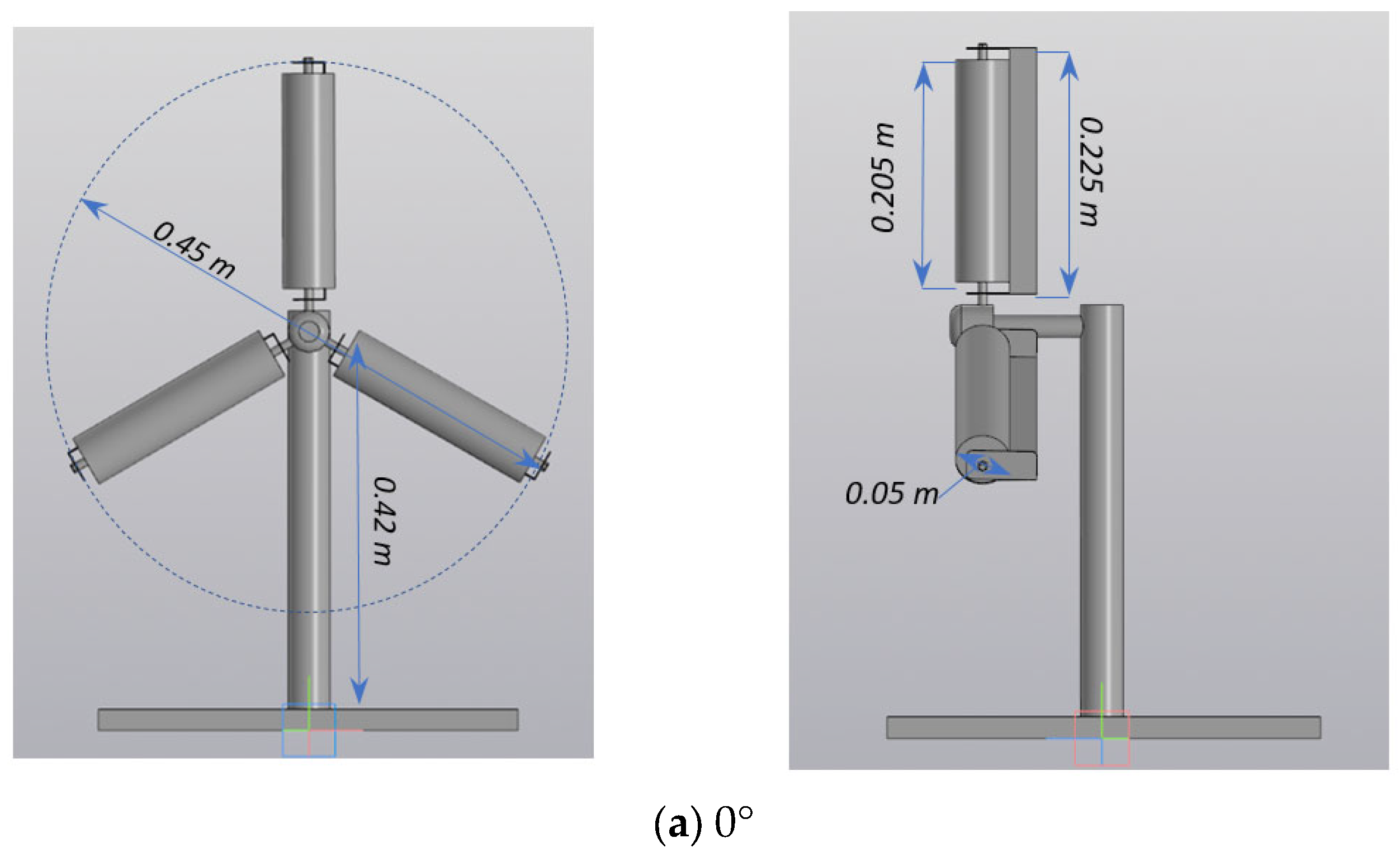
2.1. Creation of a Three-Dimensional Sample of a Wind Turbine with Three Blades

The numerical study was carried out using the Ansys Fluent 19.2 software package, based on the solution of averaged Navier–Stokes equations. The stages of numerical simulation are shown in Figure 1.

Modelling the flow around a wind wheel with combined blades is a complex numerical problem [28]. Consequently, in numerically studying the wind turbine’s aerodynamics, a geometric model was created [29,30] using the Design Modeler program and a 3D COMPASS (Figure 2).

A wind wheel with a diameter of 450 mm was created, mounted on a 420 mm long mast. The wind wheel contains 3 combined blades in the form of a cylinder. The diameter and length of the cylinder are, respectively, 50 mm and 205 mm, and the fixed blade has a length of 225 mm and a width of 25 mm.

To study the effect of the fixed blade’s inclination angle on the wind turbine’s aerodynamic characteristics, mathematical models with different fixed blade positions (0°, 15°, 30°, 45°, and 60°) were created.

2.2. A System of Equations Describing the Flow of a Liquid in a Cartesian Coordinate System

The paper considers a HAWT with 3 blades. This study was conducted using the Ansys Fluent program, which is based on the CFD method.

The initial set of parameters is shown in

Table 1. Initial parameters.

Parameter	Values
Type of air	Incompressible
Type of flow	Isothermal
Gas density	1.1691 kg/m3
Viscosity of the gas	1.84 × 10−5 kg/ms−1
Viscous Regime	Turbulent
Reynolds-Averaged Turbulence	Realisable k-epsilon
Solvers: Time-Step	0.00425 s
Maximum Inner Iterations	30

.

Since the Mach number has low M < 0.1 values, the air in this study can be considered incompressible. In this regard, the current is considered isothermal since there are minor temperature changes around the wind wheel.

The continuity equation:

$$\nabla ·\overrightarrow{U}=0$$

(1)

The momentum equation:

$$\rho {\displaystyle \frac{D\overrightarrow{U}}{Dt}}=-\nabla \mathrm{p}+\mathsf{\rho }\overrightarrow{g }+\mu {\nabla }^2\overrightarrow{U}$$

(2)

where $\rho {\displaystyle \frac{D\overrightarrow{U}}{Dt}}$—total derivative; $\nabla \mathrm{p}$—pressure gradient; $\mathsf{\rho }\overrightarrow{g }$—body force term; and $\mu {\nabla }^2\overrightarrow{U}$—diffusion term.

The equations of change in the amount of motion (Navier–Stokes equations) averaged by Reynolds:

$$\rho {\displaystyle \frac{\mathsf{\partial }{U}_i}{\mathsf{\partial }t}}+\rho U_j{\displaystyle \frac{\mathsf{\partial }{U}_i}{\mathsf{\partial }{x}_j}}=-{\displaystyle \frac{\mathsf{\partial }p}{\mathsf{\partial }{x}_i}}+\mu {\displaystyle \frac{{\mathsf{\partial }}^2{U}_i}{\mathsf{\partial }{x}_j\mathsf{\partial }{x}_i}}-{\displaystyle \frac{\mathsf{\partial }p\overline{u_i^{\prime }{u}_j^{\prime }}}{\mathsf{\partial }{x}_j}}$$

(3)

where t—time; $x_i$—Cartesian coordinates (i = 1, 2, 3); U_i—components of the averaged velocity of the liquid flow in the direction $x_i$; p—the averaged static pressure; ρ—is density; and μ—is the dynamic viscosity coefficient [31].

According to Boussinesq’s hypothesis, the Reynolds stresses on the right side are modelled as follows:

$$-\rho \overline{u_i^{\prime }{u}_j^{\prime }}={\mu }_t\left({\displaystyle \frac{{\mathsf{\partial }U}_i}{\mathsf{\partial }{x}_j}}+{\displaystyle \frac{{\mathsf{\partial }U}_j}{\mathsf{\partial }{x}_j}}\right)-{\displaystyle \frac{2}{3}}({\mu }_t{\displaystyle \frac{{\mathsf{\partial }U}_i}{\mathsf{\partial }{x}_i}}+\rho k){\delta }_{ij}$$

(4)

where $k={\displaystyle \frac{\overline{u_i^{\prime }{u}_i^{\prime }}}{2}}$—the kinetic energy of turbulent pulsations and μt—represents the dynamic turbulent viscosity coefficient.

Turbulent (vortex) and kinematic viscosity are used to relate Reynolds stresses from the Navier–Stokes equation, with an average value of $\rho \overline{u_i^{\prime }{u}_j^{\prime }}$.

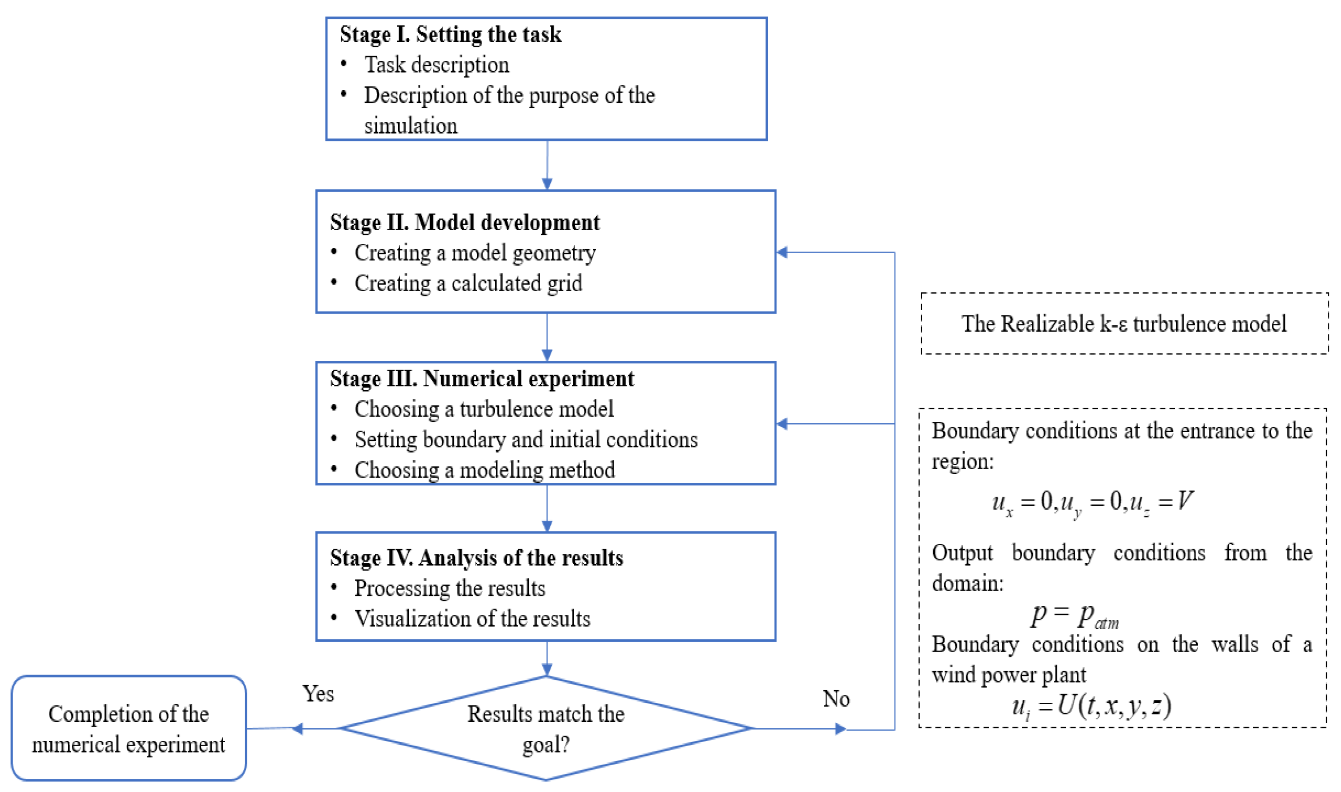
2.3. The Realisable K-Turbulence Model

To close the Navier–Stokes equations averaged by Reynolds, a realisable k-ε turbulence model was used.

The kinetic energy of turbulence k and its dissipation ε are calculated from the following transport equations:

$${\displaystyle \frac{\mathsf{\partial }}{\mathsf{\partial }t}}\left(\rho k\right)+{\displaystyle \frac{\mathsf{\partial }}{\mathsf{\partial }{x}_j}}\left(\rho k{u}_j\right)={\displaystyle \frac{\mathsf{\partial }}{\mathsf{\partial }{x}_j}}\left[(\mu +{\displaystyle \frac{{\mu }_t}{{\sigma }_k}}){\displaystyle \frac{\mathsf{\partial }k}{\mathsf{\partial }{x}_j}}\right]+G_k+G_b-\rho \epsilon +S_k$$

(5)

$${\displaystyle \frac{\mathsf{\partial }}{\mathsf{\partial }t}}\left(\rho \epsilon \right)+{\displaystyle \frac{\mathsf{\partial }}{\mathsf{\partial }{x}_j}}\left(\rho \epsilon u_j\right)={\displaystyle \frac{\mathsf{\partial }}{\mathsf{\partial }{x}_j}}\left[(\mu +{\displaystyle \frac{{\mu }_t}{{\sigma }_k}}){\displaystyle \frac{\mathsf{\partial }k}{\mathsf{\partial }{x}_j}}\right]+\rho C_{1}S\epsilon -\rho C_2{\displaystyle \frac{{\epsilon }^2}{k+\sqrt{\nu \epsilon }}}+C_1{\displaystyle \frac{\epsilon }{k}}{C}_{3\epsilon }{G}_b+S_k$$

(6)

$$C_1=max⌈0.43,{\displaystyle \frac{\eta }{\eta +5}}⌉,\eta =S{\displaystyle \frac{k}{\epsilon }},S=\sqrt{2S_{ij}{S}_{jj}}$$

(7)

In Equation (4), G_k is the generation of the kinetic energy of turbulence by the gradient of the average velocity; Gb—the generation term caused by the buoyancy effect; C_1ε, C₂, and C_3ε—constants; σk and σε are the turbulent Prandtl numbers for k and ε, respectively (σk = 1 and σε =1.2); and Sk and Sε are sources, which can be defined by the user.

The research calculations and simulations lasted a total of about 1200 h. The simulation of the layout was carried out on the combined computers of the Scientific Research Center “Alternative Energy” and the E.A. Buketov Karaganda University

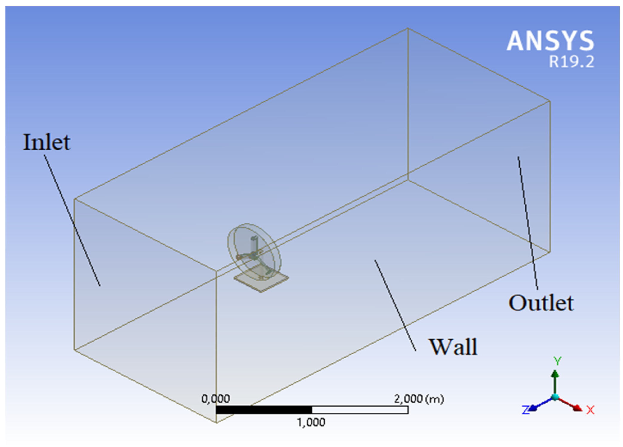
2.4. Computational Domain and Configuration

A model of a wind turbine with calculated areas for setting the boundary conditions of rotation is shown in Figure 3.

The initial stage of mathematical modelling is the creation of computational areas around the mathematical model to set boundary conditions and rotation conditions. A cylindrical subdomain (1) with a thickness of 5 mm was created around each power element to set the rotational conditions of blades. A cylindrical subdomain (2) with radius of 0.1 m around the z-axis was created around the cylindrical subdomains, as well as an area in the parallelepiped form (3), with parameters of 0.7 m; 0.7 m; 1.5 m; 0.7 m; 0.7 m; and 3 m around the cylindrical subdomain (2) (Figure 3), to rotate the conditions of the entire wind wheel.

A distinctive feature is the setting of rotation conditions; the angle between the blades is 2π/3. The rotation axis of the blades is set as (0, 1, 0), (cos(π/6), −sin (π/6), 0), (−cos (π/6), −sin (π/6), 0). The rotation of the wind wheel is set around the z-axis.

2.5. Mesh Configurations

To determine the most optimal number of grids, 3 types of grids with different numbers of cells were studied. The results for the maximum Cp at a flow rate of 15 m/s and a blade speed of 700 rpm are presented in

Table 2. Grid discretisation values.

Name	Number of Cells	Power Coefficient Cp
Mesh 1	568,410	0.274
Mesh 2	785,452	0.280
Mesh 3	890,120	0.281

.

As can be seen from Table 2, grid 2 showed a close result, and, for further calculations used in this study, the second type of grid was selected.

The finite volume grid of a wind turbine obtained in the Ansys Meshing routine is presented in Figure 4.

The selected grid type consists of 785,452 tetrahedra.

3. Results and Discussion

Below is the value of the moment of forces that affect the wind wheel. Using the formula below, the time averaging is performed:

$$〈f〉={\displaystyle \frac{1}{T}}{\int }_0^{T}f\left(t\right)dt$$

Since the rotation period of the cylinders around their own axis was 0.02 s at 300 rpm, the value of the time range of averaging was chosen from 3 to 5 s.

A line dependence of the moment of forces acting on a movable wind turbine with three blades on the velocity of the incoming flow is numerically constructed (Figure 5).

The maximum value of the moment of force is 12.7 Hm, acting on the mobile wind turbine wheel, which is observed at a wind speed of 15 m/s, and the number of rotations of the blade is 700 rpm. It was found that increasing the wind speed by 2 m/s increases the value of the moment of force by 15–19%.

The value of the C_p power coefficient is influenced by the surface velocity and wind direction [32,33].

The power coefficient C_p it is calculated by the following formula:

$$C_p={\displaystyle \frac{N_r-N_c}{N_{wf}}}$$

(8)

where $N_c=m{M}_c{\omega }_c$ is blade rotation power; $m$ is number of blades; when the blades rotate, they are exerted by a force equal to $M_c$; and ${\omega }_c$—the angular velocity generated by the rotation of the blade.

$N_{wf}={\displaystyle \frac{\rho u^{3}S}{2}}$ is the wind flow power: $\rho$ is the density of the air in the incoming flow; $S=\pi R^2$ is the area of the midsection of the rotor; $R$ is rotor’s radius; and $u$ is the incoming flow speed. $N_r=M_r{\omega }_r$ is the rotor rotation power: $M_r$ is the moment of forces acting on the movable rotor; $n$ is the number of revolutions of the cylinders; $N$ is the rotation speed of the wind wheel; and ${\omega }_r$ is the angular velocity of the free rotation of the rotor, or the rotational power of the rotor is equal to $N_r=M_r{\displaystyle \frac{2\pi n_1}{60}}$.

Figure 6 below shows the dependence power coefficient C_p from the speed (speed coefficient).

Below is a power-law speed function in which the C_p can be expressed:

$$C_p=0.1147·Z^{0.409}$$

(9)

It is determined that each value of the speed coefficient of a wind turbine with three blades corresponds to a characteristic value of the power factor, which is a linear function (8).

With a speed factor of 4.9, the wind turbine C_p is 0.28. As is known from the theory of an ideal wind turbine [34,35], the Betts–Zhukovsky wind turbine can have a maximum power coefficient C_p of 59.3% of the power of the airflow incident on it. The explanation is that the maximum efficiency of 16/27 (59.3%) is achieved when the air slows down three times when passing through the rotor. Compared with the two-bladed Magnus wind turbine [36], whose C_p is about 0.2, which is achieved by using two cylinders with a slight elongation, the data obtained indicate the increased efficiency of our installation by almost 40%.

Compared with other representatives of the Magnus wind turbine, such as a vertical one, the C_p obtained at maximum flow conditions is almost 35% higher [37].

Figure 7 and Figure 8 below show the flow patterns of a three-bladed wind wheel with a fixed blade at an angle of 0 degrees at n = 300 and 700 rpm and u = 5, 10 and 15 m/s.

The wind wheel’s rotation direction is set to clockwise in the positive direction. Defined from the results obtained (Figure 7 and Figure 8) at low speeds, the velocity field remains symmetrical relative to three planes, but with increasing air flow velocity, the formation of vortices behind the rotating blades is observed due to the formation of a turbulent wake behind the wind wheel.

These vortex formations lead to a change in the aerodynamics of the wind wheel. As the wind speed grows, the speed of rotation of the blade ends increases.

The explanation for this is the phenomenon of vortex formation increasing due to the kinetic energy of turbulence, due to the large slope of the average velocity [38].

When air passes through a rotating wind wheel, the moment of inertia decreases, thus forming a local viscous zone in which the wind speed from the wind wheel decreases. In wind turbines, this region is called a footprint, a large-scale chaotic coherent structure consisting of interconnected vortices and ordered vortex components in a given spatial range [39].

Subsequently, due to changes in wind speeds around the rotating force elements-blades in the positive direction, counterclockwise, deformation of the flow field occurs.

The pressure distribution results around the wind wheel at parameters n = 500 rpm and u = 5, 10, and 15 m/s are demonstrated in Figure 9.

As determined from Figure 9, a high-pressure area is observed on the windward side of the blade as a result of the acceleration of the flow, and a low-pressure area is formed on the leeward side of the blade.

Comparing the results with a simple cylinder, it can be seen that three-dimensional instabilities disappear, which leads to an increase in drag and a loss of lift [40].

As a result of the formation of turbulent vortices, a low-pressure area is formed. Figure 10 and Figure 11 below show the numerical simulation results of a wind wheel with a fixed blade at π/6 under different flow regimes.

In Figure 10 and Figure 11, the angle of the fixed blade is 30 degrees. A clearer image of the fixed blade can be seen above in Figure 2.

Determined from Figure 10 and Figure 11 with the deviation of the fixed blade, the entire leeward side and the edges of the blades are in the flow disruption zone, expressed in the form of the braking of the wind wheel and the premature loss of thrust at full rotation. A complex set of phenomena occurs, which are realised with the unsteady movement of the profile with the deviation of the fixed blade and the appearance of a powerful vortex flow, causing a significant increase in aerodynamic loads on the wind wheel. The results obtained do not contradict the results in [41], where the change in vortex formation modes is determined depending on the angular position of the plate on the cylinder surface.

A picture of the pressure distribution when the fixed blade is positioned at π/6 is shown in Figure 12.

Figure 12 shows the physical cause of the flow disruption at the edges of the blades, which is formed due to a positive pressure gradient along the profile chord with a boundary layer. The growth of the fixed blade location determines this interaction.

Based on the results obtained, mathematical modelling has revealed a tendency to increase drag with the growth in the angle of the plate, which leads to a decrease in the lifting force of the entire installation [42].

4. Conclusions

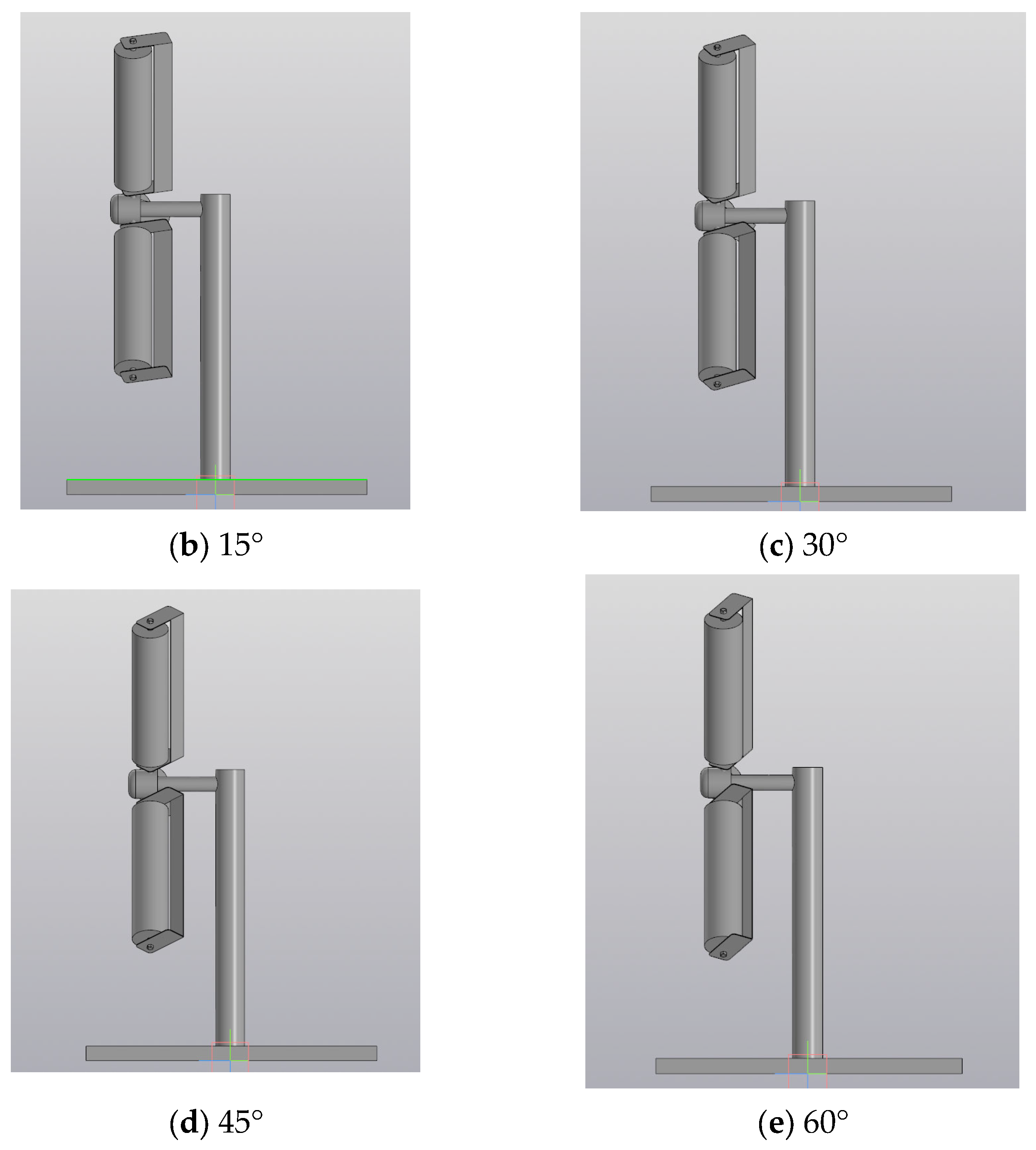
• In the course of numerical studies, a three-dimensional sample of a wind turbine with three blades was created. The sample of a wind turbine consists of combined blades designed in the form of fixed blades and cylinders, a central shaft on which the working power elements are fixed, and a mast on which the main shaft is fixed. Mathematical models with different positions of the fixed blade were created (0°, 15°, 30°, 45°, and 60°), with further study of their influence on the hydrodynamic features and parameters of the entire installation.
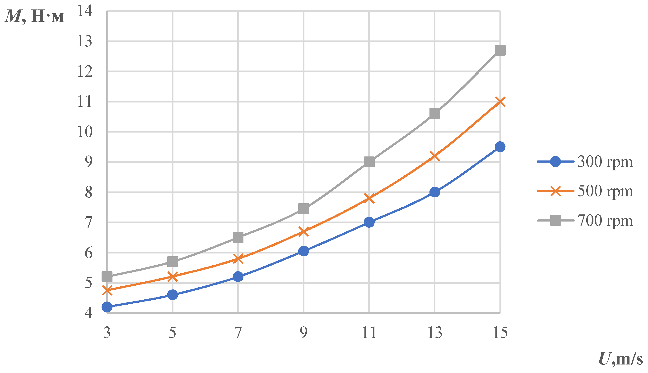
• A line of the dependence of the moment of forces acting on a movable wind turbine with three blades on the velocity of the incoming flow was constructed. For a three-bladed wind turbine, the dependence of the influence of the rotation frequency on the value of the power coefficient C_p was obtained. The wind speed value was determined to correspond to a certain value of C_p. The developed wind turbine with three combined blades has a power coefficient of 0.28. Adding a fixed blade increases the efficiency of the wind turbine by 35–40% when compared with the results of other authors.
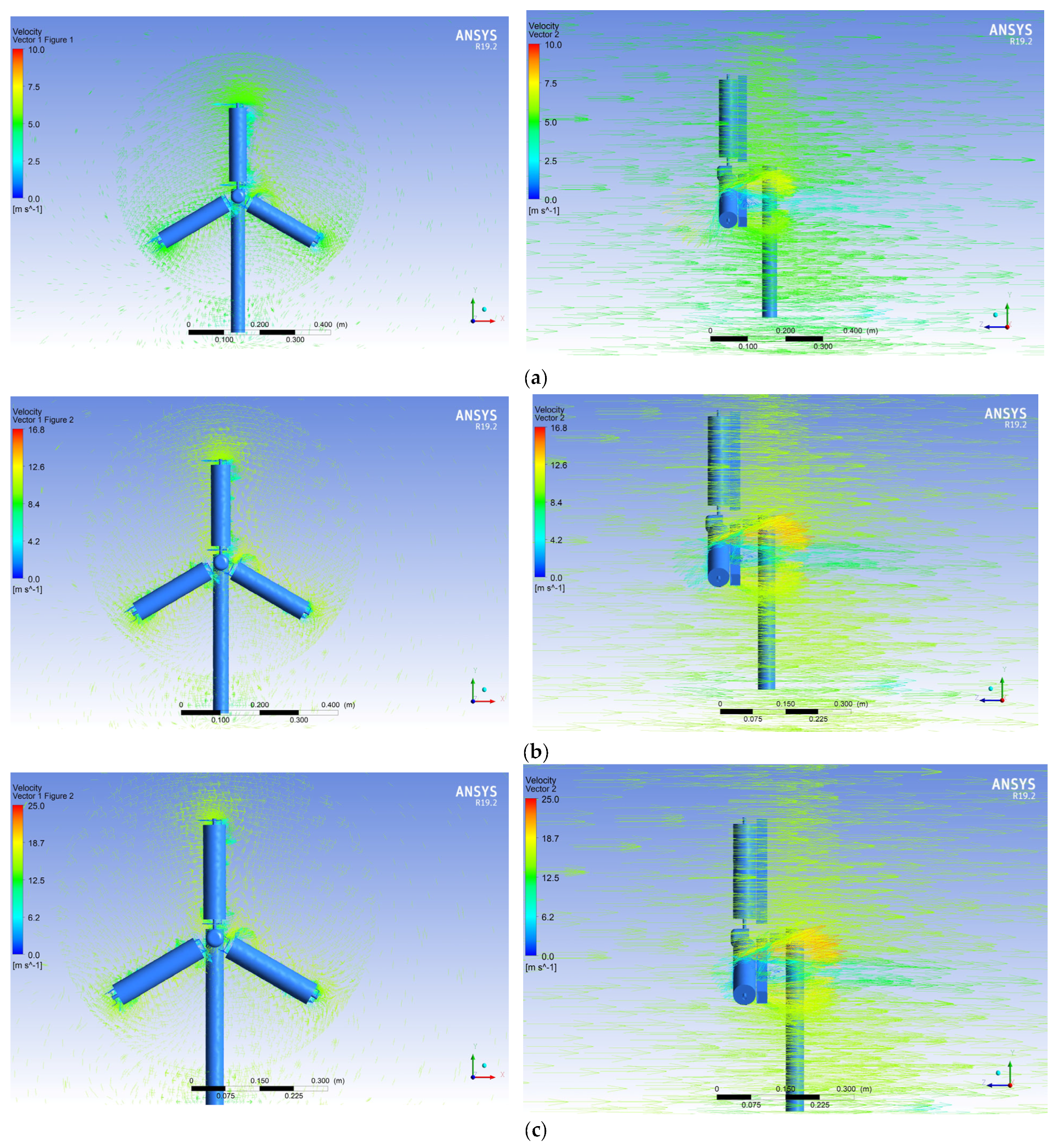
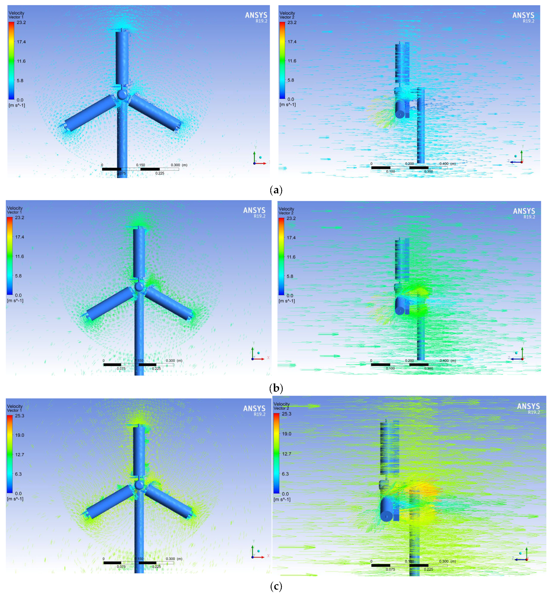
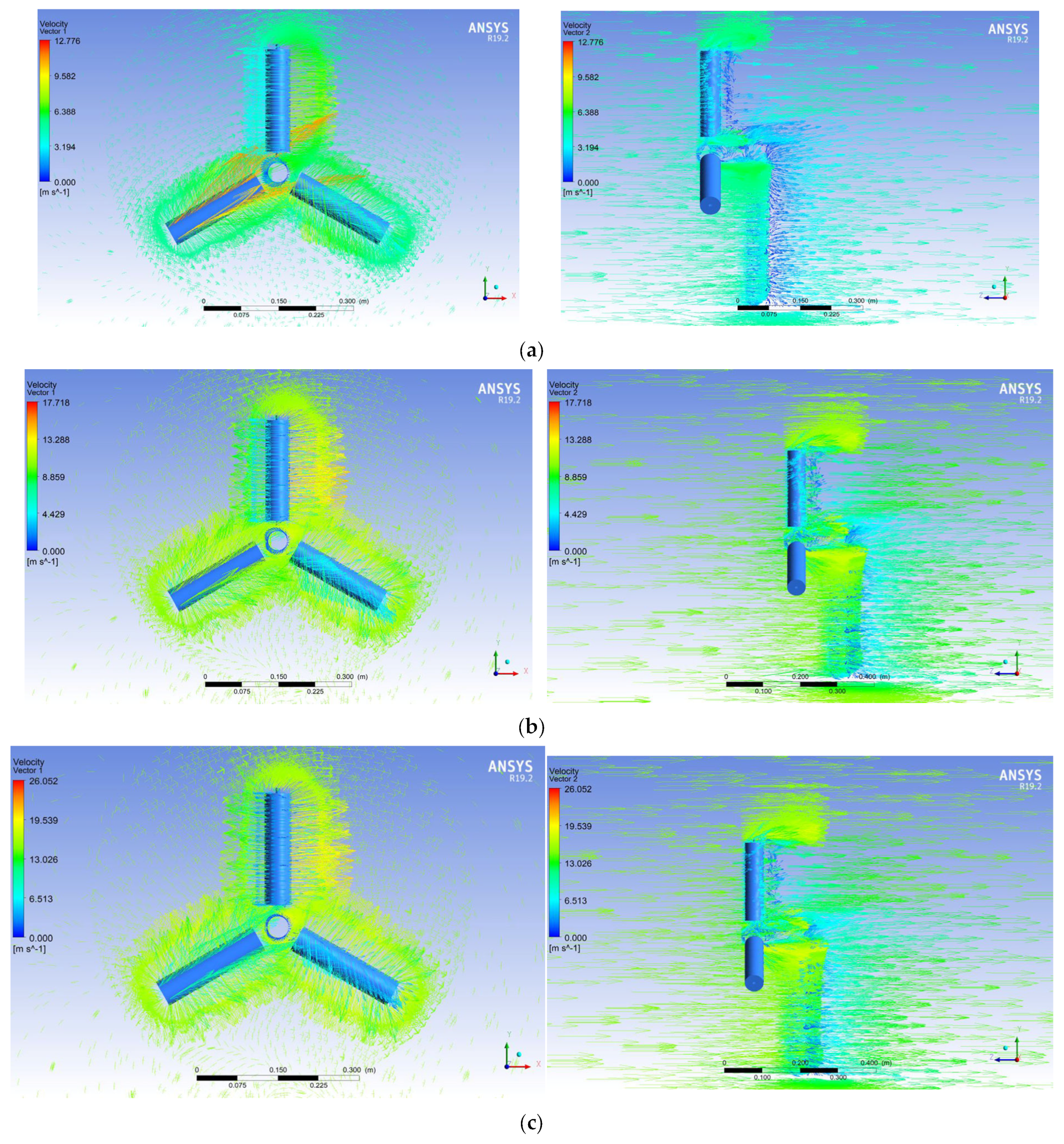
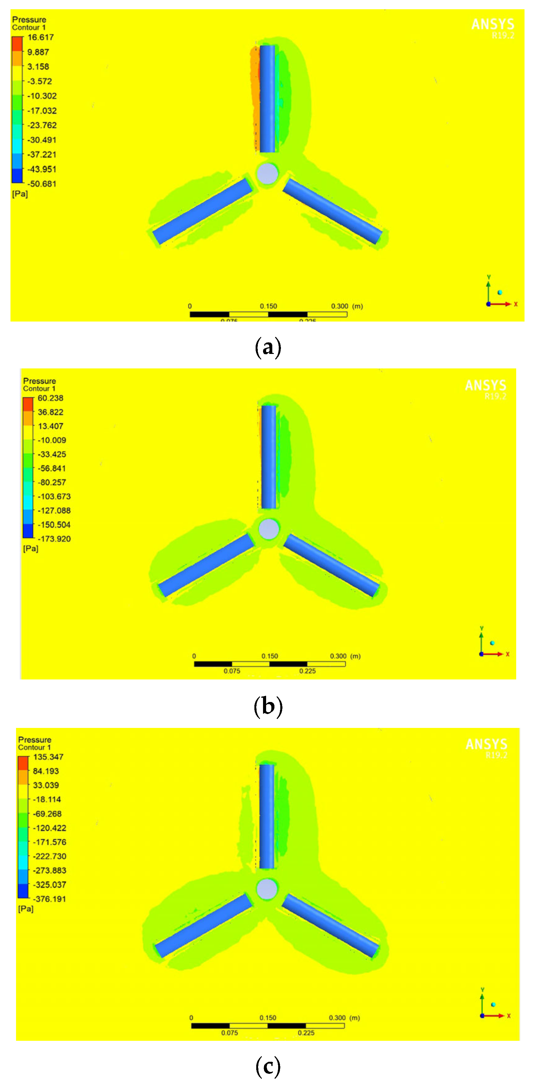
• When the fixed blade was positioned at angles of 0° and π/6, the effect on the distribution patterns of the velocity vector around a rotating wind wheel with three blades was studied. When the fixed blade was positioned at π/6, and at maximum rotational speeds, a flow disturbance was observed due to increased resistance. As a result, there is a decrease in the lifting force of the blades, which subsequently leads to a reduction in efficiency. Based on this, the favourable angle of the fixed blade is an angle of 0 degrees for both two-bladed and three-bladed wind turbines. The pressure distribution patterns around a rotating wind wheel with a fixed blade were obtained at 0 and 30 degrees. Based on the pressure distribution results, it is determined that when the fixed blade is located at π/6, the matrix layer is separated due to the braking of the wind wheel and an unfavourable pressure gradient. As a result, it was found that the location of the fixed blade at an angle of 0 degrees for the entire wind wheel is favourable for obtaining the optimal aerodynamic performance of all wind turbines.

The use of renewable energy sources makes it possible to move away from import dependence, allowing countries to diversify their economies and protect them from fluctuations in market prices for fossil fuels while stimulating inclusive economic growth, job creation, and poverty reduction. The effective use of wind turbines is most attractive, since the natural balance of energy on the planet is not disturbed, and, at the same time, a waste-free, environmentally friendly energy production technology is used for various purposes: battery charging and electricity storage and energy supply to various facilities and remote areas (street lighting, heating of buildings, houses, farms, electrification of field mills, etc., and granaries, pastures, apiaries, etc.).

The results obtained have great potential in future research in the field of efficient use of renewable energy sources (RES) in the form of assistance for creating and developing efficient wind turbines for low wind speeds. The developed wind turbine does not have a detrimental effect on the environment, flora, or fauna, since the wind turbine size belongs to the category of small installations designed for minimum wind speeds.

References

1. Moussa, M.O. Experimental and numerical performances analysis of a small three-blade wind turbine. Energy 2020, 203, 117807. [Google Scholar] [CrossRef]
2. Ahmed, S.D.; Al-Ismail, F.S.; Shafiullah, M.; Al-Sulaiman, F.A.; El-Amin, I.M. Grid integration challenges of wind energy: A review. IEEE Access 2020, 8, 10857–10878. [Google Scholar] [CrossRef]
3. IRENA—International Renewable Energy Agency. Available online: https://www.iaea.org/about/partnerships/irena (accessed on 1 July 2024).
4. Elkodama, A.; Ismaiel, A.; Abdellatif, A.; Shaaban, S.; Yoshida, S.; Rushdi, M.A. Control methods for horizontal axis wind turbines (HAWT): State-of-the-art review. Energies 2023, 16, 6394. [Google Scholar] [CrossRef]
5. Ghorani, M.M.; Karimi, B.; Mirghavami, S.M.; Saboohi, Z. A numerical study on the feasibility of electricity production using an optimised wind delivery system (Invelox) integrated with a Horizontal axis wind turbine (HAWT). Energy 2023, 268, 126643. [Google Scholar] [CrossRef]
6. Mirsane, R.S.; Rahimi, M.; Torabi, F. Development of a novel analytical wake model behind HAWT by considering the nacelle effect. Energy Convers. Manag. 2024, 301, 118031. [Google Scholar] [CrossRef]
7. Roga, S.; Bardhan, S.; Kumar, Y.; Dubey, S.K. Recent technology and challenges of wind energy generation: A review. Sustain. Energy Technol. Assess. 2022, 52, 102239. [Google Scholar] [CrossRef]
8. Sharma, D.; Goyal, R. Methodologies to improve the performance of vertical axis wind turbine: A review on stall formation and mitigation. Sustain. Energy Technol. Assess. 2023, 60, 103561. [Google Scholar] [CrossRef]
9. Li, G.; Li, Y.; Li, J.; Huang, H.; Huang, L. Research on dynamic characteristics of vertical axis wind turbine extended to the outside of buildings. Energy 2023, 272, 127182. [Google Scholar] [CrossRef]
10. Al-Rawajfeh, M.A.; Gomaa, M.R. Comparison between horizontal and vertical axis wind turbine. Int. J. Appl. 2023, 12, 13–23. [Google Scholar] [CrossRef]
11. Roy, S.; Das, B.; Biswas, A. A comprehensive review of the application of bio-inspired tubercles on the horizontal axis wind turbine blade. Int. J. Environ. Sci. Technol. 2023, 20, 4695–4722. [Google Scholar] [CrossRef]
12. Li, M.; Dirik, Y.; Oterkus, E.; Oterkus, S. Shape sensing of NREL 5 MW offshore wind turbine blade using iFEM methodology. Ocean. Eng. 2023, 273, 114036. [Google Scholar] [CrossRef]
13. Morina, R.; Akansu, Y.E. The Effect of Leading-Edge Wavy Shape on the Performance of Small-Scale HAWT Rotors. Energies 2023, 16, 6405. [Google Scholar] [CrossRef]
14. Shankar, R.N.; Kumar, L.R.; Ramana, M.V. Design and fabrication of horizontal axis wind turbine. Int. J. Res. Anal. Rev. (IJRAR) 2019, 6, 545–549. [Google Scholar]
15. Ranjan, R.; Pandey, R.; Singh, R.; Mohanty, S. Design and Modeling of Small Horizontal Axis Wind Turbine Blade for Low Wind Speed Characteristics. In International Conference on Machine Intelligence for Research & Innovations; Springer Nature: Singapore, 2023; pp. 271–279. [Google Scholar]
16. Zareian, M.; Rasam, A.; Tari, P.H. A detached-eddy simulation study on assessing the impact of extreme wind conditions on load and wake characteristics of a horizontal-axis wind turbine. Energy 2024, 299, 131438. [Google Scholar] [CrossRef]
17. Oukassou, K.; El Mouhsine, S.; El Hajjaji, A.; Kharbouch, B. Comparison of the power, lift and drag coefficients of wind turbine blade from aerodynamics characteristics of Naca0012 and Naca2412. Procedia Manuf. 2019, 32, 983–990. [Google Scholar] [CrossRef]
18. Yan, C.; McDonald, J.G. Hyperbolic equivalent k-ϵ and k-ω turbulence models for moment-closures. J. Comput. Phys. 2023, 476, 111881. [Google Scholar] [CrossRef]
19. De la Cruz-Ávila, M.; De León-Ruiz, J.E.; Carvajal-Mariscal, I.; Klapp, J. CFD Turbulence Models Assessment for the Cavitation Phenomenon in a Rectangular Profile Venturi Tube. Fluids 2024, 9, 71. [Google Scholar] [CrossRef]
20. Rahman, M.M.; Karim, M.M.; Alim, M.A. Numerical investigation of unsteady flow past a circular cylinder using 2-D finite volume method. J. Nav. Archit. Mar. Eng. 2007, 4, 27–42. [Google Scholar] [CrossRef]
21. Umar, D.A.; Yaw, C.T.; Koh, S.P.; Tiong, S.K.; Alkahtani, A.A.; Yusaf, T. Design and optimization of a small-scale horizontal axis wind turbine blade for energy harvesting at low wind profile areas. Energies 2022, 15, 3033. [Google Scholar] [CrossRef]
22. Kriswanto; Setiawan, M.A.B.; Al-Janan, D.H.; Naryanto, R.F.; Roziqin, A.; Firmansyah, H.N.; Setiadi, R.; Darsono, F.B.; Setiyawan, A.; Jamari. Power Optimization of The Horizontal Axis Wind Turbine Capacity of 1 MW on Various Parameters of The Airfoil, an Angle of Attack, and a Pitch Angle. J. Adv. Res. Fluid Mech. Therm. Sci. 2023, 103, 141–156. [Google Scholar] [CrossRef]
23. Kassa, B.Y.; Baheta, A.T.; Beyene, A. Current trends and innovations in enhancing the aerodynamic performance of small-scale, horizontal axis wind turbines: A review. ASME Open J. Eng. 2024, 3. [Google Scholar] [CrossRef]
24. Marzuki, O.F.; Mohd Rafie, A.S.; Romli, F.I.; Ahmad, K.A. Magnus wind turbine: The effect of sandpaper surface roughness on cylinder blades. Acta Mech. 2018, 229, 71–85. [Google Scholar] [CrossRef]
25. Ikezawa, Y.; Hasegawa, H.; Ishido, T.; Haniu, T.; Murakami, N. Three-dimensional flow field around a rotating cylinder with spiral fin for Magnus wind turbine. J. Flow Vis. Image Process. 2018, 25. [Google Scholar] [CrossRef]
26. Demidova, G.L.; Anuchin, A.; Lukin, A.; Lukichev, D.; Rassõlkin, A.; Belahcen, A. Magnus wind turbine: Finite element analysis and control system. In Proceedings of the 2020 International Symposium on Power Electronics, Electrical Drives, Automation and Motion (SPEEDAM), Sorrento, Italy, 24–26 June 2020; IEEE: Piscataway, NJ, USA, 2020; pp. 59–64. [Google Scholar]
27. Dyusembaeva, A.N.; Tleubergenova, A.Z.; Tanasheva, N.K.; Nussupbekov, B.R.; Bakhtybekova, A.R.; Kyzdarbekova, S.S. Numerical investigation of the flow around a rotating cylinder with a plate under the subcritical regime of the Reynolds number. Int. J. Green Energy 2024, 21, 973–987. [Google Scholar] [CrossRef]
28. Tanasheva, N.; Tleubergenova, A.; Dyusembaeva, A.; Satybaldin, A.; Mussenova, E.; Bakhtybekova, A.; Shuyushbayeva, N.; Kyzdarbekova, S.; Suleimenova, S.; Tussypbayeva, A. Determination of the aerodynamic characteristics of a wind power plant with a vertical axis of rotation. East. Eur. J. Enterp. Technol. 2023, 122, 36. [Google Scholar] [CrossRef]
29. Siddiqui, M.S.; Khalid, M.H.; Badar, A.W.; Saeed, M.; Asim, T. Parametric analysis using CFD to study the impact of Geometric and numerical modeling on the performance of a small-scale horizontal axis wind turbine. Energies 2022, 15, 505. [Google Scholar] [CrossRef]
30. Regodeseves, P.G.; Morros, C.S. Unsteady numerical investigation of the full geometry of a horizontal axis wind turbine: Flow through the rotor and wake. Energy 2020, 202, 117674. [Google Scholar] [CrossRef]
31. Heinz, S.; Mokhtarpoor, R.; Stoellinger, M. Theory-based Reynolds-averaged Navier–Stokes equations with large eddy simulation capability for separated turbulent flow simulations. Phys. Fluids 2020, 32. [Google Scholar] [CrossRef]
32. Liu, M.; Wang, X. Three-dimensional wind field construction and wind turbine siting in an urban environment. Fluids 2020, 5, 137. [Google Scholar] [CrossRef]
33. Tanasheva, N.K.; Bakhtybekova, A.R.; Shuyushbayeva, N.N.; Tussupbekova, A.K.; Tleubergenova, A.Z. Calculation of the aerodynamic characteristics of a wind-power plant with blades in the form of rotating cylinders. Tech. Phys. Lett. 2022, 48, 51–54. [Google Scholar] [CrossRef]
34. Sørensen, J.N. General Momentum Theory for Horizontal Axis Wind Turbines; Springer: New York, NY, USA, 2016; Volume 4. [Google Scholar]
35. Okulov, V.L.; Van Kuik, G.A. The Betz–Joukowsky limit: On the contribution to rotor aerodynamics by the British, German and Russian scientific schools. Wind Energy 2012, 15, 335–344. [Google Scholar] [CrossRef]
36. Richmond-Navarro, G.; Calderón-Munoz, W.R.; LeBoeuf, R.; Castillo, P. A Magnus wind turbine power model based on direct solutions using the Blade Element Momentum Theory and symbolic regression. IEEE Trans. Sustain. Energy 2016, 8, 425–430. [Google Scholar] [CrossRef]
37. Khadir, L.; Mrad, H. Numerical investigation of aerodynamic performance of Darrieus wind turbine based on the magnus effect. Int. J. Multiphysics 2015, 9, 383–396. [Google Scholar] [CrossRef]
38. Tleubergenova, A.Z.; Tanasheva, N.K.; Shaimerdenova, K.M.; Kassymov, S.S.; Bakhtybekova, A.R.; Shuyushbayeva, N.N.; Uzbergenova, S.Z.; Ranova, G.A. Mathematical modeling of the aerodynamic coefficients of a sail blade. Adv. Aerodyn. 2023, 5, 14. [Google Scholar] [CrossRef]
39. Alrowwad, I.; Wang, X.; Zhou, N. Numerical modelling and simulation analysis of wind blades: A critical review. Clean Energy 2024, 8, 261–279. [Google Scholar] [CrossRef]
40. Bai, X.; Ji, C.; Grant, P.; Phillips, N.; Oza, U.; Avital, E.J.; Williams, J.J. Turbulent flow simulation of a single-blade Magnus rotor. Adv. Aerodyn. 2021, 3, 19. [Google Scholar] [CrossRef]
41. Zhao, M. A review of recent studies on the control of vortex-induced vibration of circular cylinders. Ocean. Eng. 2023, 285, 115389. [Google Scholar] [CrossRef]
42. Ma, Y.; Rashidi, M.M.; Yang, Z.G. Numerical simulation of flow past a square cylinder with a circular bar upstream and a splitter plate downstream. J. Hydrodyn. 2019, 31, 949–964. [Google Scholar] [CrossRef]
Figure 1. The stages of solving the task in the Fluent 19.2 software package.
Energies 17 04054 g001
Figure 2. A model of a wind turbine with a different arrangement of a fixed blade.
Energies 17 04054 g002aEnergies 17 04054 g002b
Figure 3. Mathematical model of a 3-blade wind turbine.
Energies 17 04054 g003
Figure 4. Finite volume grid.
Energies 17 04054 g004
Figure 5. Moment of forces acting on a movable wind wheel with three blades.
Energies 17 04054 g005
Figure 6. Changing the power coefficient Cp depending on the speed coefficient of the wind turbine.
Energies 17 04054 g006
Figure 7. The flow pattern of a wind turbine when the fixed blade is positioned at an angle of 0 degrees at n = 300 rpm: (a) at u = 5 m/s; (b) u = 10 m/s; and (c) u = 15 m/s.
Energies 17 04054 g007
Figure 8. The flow pattern of a wind turbine when the fixed blade is positioned at an angle of 0 degrees at n = 700 rpm: (a) at u = 5 m/s; (b) u = 10 m/s; and (c) u = 15 m/s.
Energies 17 04054 g008
Figure 9. Result of investigation (pressure distribution) of a fixed blade at an angle of 0 degrees to the cylinder at parameters n = 500 revolutions per minute: (a) at u = 5 m/s; (b) u = 10 m/s; (c) u = 15 m/s.
Energies 17 04054 g009
Figure 10. The velocity field around the rotating wind wheel when the fixed blade is positioned at an angle of 30 degrees at n = 300 rpm: (a) at u = 5 m/s; (b) u = 10 m/s; and (c) u = 15 m/s.
Energies 17 04054 g010
Figure 11. The velocity field around the rotating wind wheel when the fixed blade is positioned at an angle of 30 degrees at n = 700 rpm: (a) at u = 5 m/s; (b) u = 10 m/s; and (c) u = 15 m/s.
Energies 17 04054 g011
Figure 12. A picture of the pressure distribution when the fixed blade is positioned at an angle of 30 degrees and at n = 500 rpm: (a) at u = 5 m/s; (b) u = 10 m/s; and (c) u = 15 m/s.
Energies 17 04054 g012