Abstract
Understanding the mechanisms of snap-off during gas–liquid immiscible displacement is of great significance in the petroleum industry to enhance oil and gas recovery. In this work, based on the original pseudo-potential lattice Boltzmann method, we improved the fluid–fluid force and fluid–solid force scheme. Additionally, we integrated the Redlich–Kwong equation of state into the lattice Boltzmann model and employed the exact difference method to incorporate external forces within the lattice Boltzmann framework. Based on this model, a pore–throat–pore system was built, enabling gas–liquid to flow through it to investigate the snap-off phenomenon. The results showed the following: (1) The snap-off phenomenon is related to three key factors: the displacement pressure, the pore–throat length ratio, and the pore–throat width ratio. (2) The snap-off phenomenon occurs only when the displacement pressure is within a certain range. When the displacement pressure is larger than the upper limit, the snap-off will be inhibited, and when the pressure is less than the lower limit, the gas–liquid interface cannot overcome the pore–throat and results in a “pinning” effect. (3) The snap-off phenomenon is controlled using the pore–throat structures: e.g., length ratio and the width ratio between pore and throat. It is found that the snap-off phenomenon could easily occur in a “long-narrow” pore–throat system, and yet hardly in a “short-wide” pore–throat system.
1. Introduction
The immiscible displacement in complex porous media plays a crucial role in two-phase flow and holds significant research significance in the field of enhanced oil/gas recovery, such as gas-driven processes, gas–water alternation, and foam-based driving [1,2,3,4,5]. During gas driving, a complex gas–liquid immiscible mode will form after continuous gas injection into the reservoir. Generally, the gas is a non-wetting phase, and a liquid film acting as the wetting phase will stick on the walls of the pores. The existence of liquid film may cause the phenomenon of snap-off. Therefore, it is necessary to understand the gas–liquid flow state in the pore–throat system to further study the snap-off mechanism during the gas–liquid immiscible displacement.
Lots of theoretical and experimental works have studied the snap-off mechanism in gas–liquid two-phase flow process. In terms of theoretical analysis, Roof [6] established a static criterion for predicting snap-off based on the capillary pressure balance at pore throats. He pointed out that when the minimum throat radius is less than half of the pore radius, the wetting phase refluxes along the pore wall, which leads to a snap-off of the non-wetting phase. Gauglitz et al. [7] also proposed the snap-off criterion for a constricted cylindrical pore–throat system, and pointed out that the capillary number has a certain impact on the occurrence of snap-off and its influence depends on the pore–throat width radio. Ransohoff et al. [8] further provided static snap-off criteria for pores with square and triangular sections, and found that snap-off is more likely to occur in the throat with non-circular sections. However, most of the criteria above only considered the static mechanical equilibrium at the pore throat without considering the influence of dynamic flow for the fluids. Tsai et al. [9] found that the bubble will not snap-off if the capillary number is too large or too small. Deng et al. [10,11] by expanding the static snap-off criteria of circular and non-circular neck constricting pore–throat systems, found that the previous static criteria were too conservative in predicting snap-off, and the high capillary number would inhibit the occurrence of snap-off even if the throat system reached the static criteria for the occurrence of snap-off. In terms of experiments, with the development of the microfluidic model, a large number of scholars use it to carry out visual experiments on the phenomenon of snap-off in two-phase flow. Tian et al. [12] used 2D micromodels to study the phenomenon of snap-off during gas–water flow and verified the static criterion proposed by Roof et al. By using a 2D rectangular cross-section micromodel, Cha et al. [13] studied the mechanism of bubble snap-off and obtained a good consistency with the theoretical model they proposed. Tetteh et al. [14] observed the oil phase snap-off in the course of low-salinity water flooding through the use of the microfluidic model. Wu et al. [15] experimentally studied the snap-off in snakelike pore–throat structures, and believed that throat length and width had a certain influence on snap-off.
Compared with experiments, numerical simulation can better understand and predict the gas–liquid two-phase flow state and snap-off at the pore scale. There is pore network modeling (PNM) [16], smoothed particle hydrodynamics (SPH) [17], density functional hydrodynamics (DFH) [18], the volume-of-fluid method (VOF) [19] and the lattice Boltzmann method (LBM) [20] to simulate multiphase flow at the pore scale. Some researchers used VOF to study the snap-off in the constricted pore–throat systems. Considering the influence of dynamic factors, Raeini et al. [21] used the VOF method to study the star-shaped throat section for snap-off. Starnoni et al. [22] adopted the VOF method to study the effects of the contact angle and viscosity ratio for snap-off; they found that the threshold contact angle increases with diminishing of the roundness of the cross-section, and the increase in viscosity ratio would also reduce the threshold contact angle. Zhang et al. [23] studied the square section throat through the VOF method. It is concluded that high capillary numbers and a high viscosity ratio can effectively inhibit the occurrence of snap-off. Cha et al. [13] used the VOF method to simulate the snap-off of a rectangular cross-section and provided the conditions of the pore–throat width ratio for the occurrence of snap-off. However, when using the VOF method it is difficult to calculate the normal direction and curvature of the interface accurately, and the interface reconstruction method is complex, which makes it difficult to extend to higher dimensions [24]. LBM is a mesoscopic numerical simulation between the micro molecular dynamics simulation method and the macroscopic traditional numerical simulation method. Compared with interface tracking or interface capture methods such as the VOF method, the gas–liquid interface in LBM can be generated, evolved and migrated automatically without any interface tracking or interface capture technology [25], and can directly deal with the force between the fluid and fluid as well as the force between the fluid and solid wall [26]. At present, multiphase LBMs can be divided into four categories, including a color-gradient model [27], a pseudo-potential model [28], a free energy model [29] and a phase-field model [30]. Based on the color-gradient model, Zhang Lei et al. [31] simulated an immiscible displacement process in a pore–throat system, and believed that with the increasing heterogeneity of porous media, the fluid is prone to snap-off. Zhao Yulong et al. [32] simulated the flow process of tight gas flooding formation water under high temperature and high pressure, and found that a large number of connected micro-channels in porous media were occupied by blocked water. Alpak et al. [33] used the phase-field model to simulate the two-phase displacement process in 3D constricted pores and observed the snap-off, which was consistent with the Roof static criterion. However, the viscosity difference in the simulated two-phase fluid was not large enough to reflect the viscosity ratio of gas–liquid two phases. Wei et al. [34] used the pseudo-potential model to simulate the process of a single bubble passing through the throat, and observed the snap-off. Zhang et al. [35] used the improved two-component pseudo-potential model to simulate the gas–water flooding process and successfully captured the existence of water film on the throat wall. They believed that the thickness of the liquid film on the wall could not be ignored in the process of gas–water two-phase flow at the micro/nano-scale.
However, the current research on the snap-off is usually based on the neck of the pore–throat system, where the effect of the wall–liquid film thickness is not very obvious. Meanwhile, the macroscopic VOF method cannot fully characterize the wall–liquid film interaction. In this paper, based on the original pseudo-potential LBM, we improve the force scheme between fluids and add fluid–solid force to capture the liquid film variation on the throat wall. The influence of the liquid film on the flow state of the gas–liquid flow during the phase displacement is studied. Furthermore, the effects of displacement pressure difference (capillary number), throat length and width on liquid film thickness and flow state is probed. This work provides a theoretical and simulation basis for the characterization of the snap-off mechanism in complex porous media.
2. Materials and Methods
2.1. Analysis on Mechanisms and Factors of Snap-Off
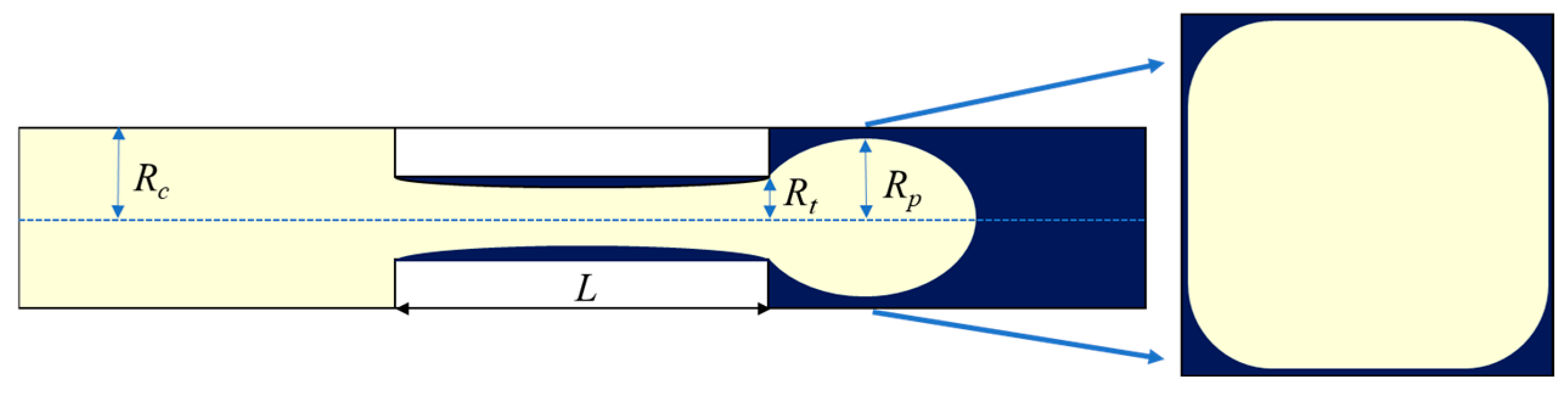
Based on Roof’s mechanism, which supports that the capillary force Pc-neck of the throat is greater than Pc-front of the leading edge, Ransohoff et al. [8] proposed the static snap-off criterion of the square pore–throat system, and the core hypothesis is that the wetting phase is the main flow mode in the corner of the square throat system, as shown in Figure 1. Ignoring the effect of liquid film on the wall, the snap-off judgement criterion of the throat system of the constricted square can be expressed as the following:
where Rc, Rt, Rzt are the radius of the pore curvature, throat curvature, transverse throat curvature, respectively. Cm is dimensionless curvature, which is related to the shape of pore section. Based on the minimum surface energy model, Cm = 1.89 in square pores, given by Ransohoff et al. [8]. Regardless of 1/Rzt, when pore shrinkage is gentle, Rc > 1.89Rt.
Figure 1.
Schematic diagram of gas–liquid two-phase flow. (Yellow is the gas phase and blue is the water phase).
An improved pseudo-potential model is used to verify the applicability of the static criterion proposed by Ransohoff et al. [8]. To facilitate the comparison of the simulation results with this criterion, the dimensionless pore–throat length ratio and width ratio are defined to characterize the change in pore structure, which are expressed as the following:
where Lp is the length of the entire pore–throat system, and L is the length of the throat. Based on this, we can find the static criterion of snap-off R* ≤ 0.53.
2.2. Lattice Boltzmann Method
The Bhatnagar-Gross-Krook (BGK) collision process can be expressed by characterizing the fluid motion with the discrete density distribution [36], which can be written as follows:
where fi(x,t) is the density distribution function along i direction; Δx and Δt represent grid step and time step, respectively; τ denotes the relaxation time, whose expression is showed in Equation (2).
where is the local speed of sound, and ν represents the kinetic viscosity. In Equation (1), ei is defined to be the discrete velocity in each direction, and for the D2Q9 model (“D2” indicates that the model is applied in two spatial dimensions, while “Q9” signifies that there are nine discrete velocities considered in the LBM) [37], it is expressed as the following:
The equilibrium density distribution is calculated using the following equation:
where wi is a weight factor; for the D2Q9 model, wi = 4/9 when i = 0; wi = 1/9 when i = 1~4; wi = 1/36 when i = 5~8. The macroscopic density ρ and velocity u are calculated as follows:
The original pseudo-potential model achieves phase separation through incorporating inter-particle forces within the fluid system. The forces between fluids in the pseudo-potential model are defined as follows [28]:
where G is the Green function; ψ(x,t) is the effective mass, which is defined as ψ(ρ) = ρ0[1 − exp(−ρ/ρ0)], and ρ0 = 1 is the reference density. Given the forces between the particles in the first layer, the formula can be simplified as follows:
where g is the control parameter of interaction intensity between fluids, w(|ei|2) is weight coefficient, |ei|2 = 1, w(|ei|2) = 1/3; |ei|2 = 2, w(|ei|2) = 1/12. The equation of state of the pseudo-potential model can be expressed as the following [28]:
However, using the above equation will lead to a thermodynamic inconsistency, and the maximum density ratio and viscosity are both within 10 during the simulation. Therefore, a model combining the real fluid equation of state with the pseudo-potential model was proposed by Yuan et al. [38] to improve its accuracy. In this paper, we use the Redlich–Kwong equation of state (RK EOS) to characterize the gas–liquid two-phase. Firstly, the RK EOS is a relatively simple yet accurate model for describing the thermodynamic properties of non-ideal gases, especially in the context of dense fluids or near-critical conditions. Secondly, it offers a good compromise between computational complexity and accuracy, making it suitable for the numerical simulations conducted in this study. Additionally, the RK EOS has been widely used and validated in the literature, providing a solid foundation for our investigations [39]. The RK EOS is defined as the following:
where pEOS is the pressure of the actual fluid, R is gas constant, T is the temperature of the system, ρ is the density of the actual fluid, and a as well as b are both critical parameters (a = 0.42748R2Tc2.5/pc, b = 0.08662RTc/pc). Huang et al. [40] gave the parameter values, where a = 2/49, b = 2/21, R = 1, Tc = 0.1961, pc = 0.1784, ρc = 2.9887. The following formula can be used to calculate the effective mass after adding the RK equation:
It is worth noting that g will be eliminated in the calculation of force (Equation (8)), so it ensures that the sign in the square root sign is positive. Therefore, g = −1 is chosen in the simulation. In this paper, a modified force scheme proposed by Gong et al. [41] is adopted to reduce the false velocity at the interface between the two phases, as shown in Equation (9).
Furthermore, Chen et al. [42] proposed a simplified formula considering the interaction between the nearest the next-nearest nodes.
where β is an adjusting parameter, which can improve the thermodynamic consistency of the model and reduce the false velocity by changing β. If we only consider the forces of the nodes in the first layer, Equation (9) is further extended to the following [14]:
It is also called E4 force scheme. γ1 and γ2 are the discretized coefficients, where γ1 = 1/3 and γ2 = 1/12. The readers can refer to Mukherjee et al. [43]’s study of extending the forces to E6/E8 force schemes to obtain lower false velocities and more accurate interfacial tensions.
The force between fluid and wall is similar to that between fluids [39].
where the function to determine the fluid node and the wall surface is s(x + eiΔt,t). If x + eiΔt is 1 in the solid node, the corresponding value in the fluid node is 0. ρw is the wall density, which can be adjusted to simulate different contact angles. In the traditional LBM, external forces are often approximated using a simple forcing term, which may introduce discretization errors. The exact difference method (EDM) [44] addresses this issue through providing a more accurate way to account for these external forces. The key idea of the EDM is to calculate the exact difference between the equilibrium distribution functions in the presence and absence of external forces (∆fi(x, t)). This exact difference is then added to the collision operator in the LBM, ensuring that the influence of external forces is accurately captured. For adding fluid–fluid force and fluid–solid force, this paper adopts the exact difference method (EDM) scheme to deal with the external forces, which can be written as the following:
where Ftotal represents the sum of the fluid–fluid force and the fluid–solid force. EDM is one of the most common external force processing formats and can be adapted to a wide temperature range.
3. Model Verification
3.1. Verification of Thermodynamic Consistency
Thermodynamic inconsistency is the main problem in pseudo-potential models, which will directly affect the calculation accuracy of the gas–liquid density ratio and interfacial tension. Therefore, evaluating the model is the first thing to be conducted. Since the capillary pressure will have a certain impact on the gas–liquid density, we use the gas–liquid model with a hypothetical flat interface to study the gas–liquid coexistence density, and compare it with Maxwell’s theoretical results to evaluate the thermodynamic consistency. First, a 31 × 201 lattice space is established, and periodic boundaries are set in both x and y directions. The gas–liquid coexistence density can be simulated by only changing the temperature. Also, the density initialization method of Huang et al. [45] can improve the numerical stability, which is expressed as the following:
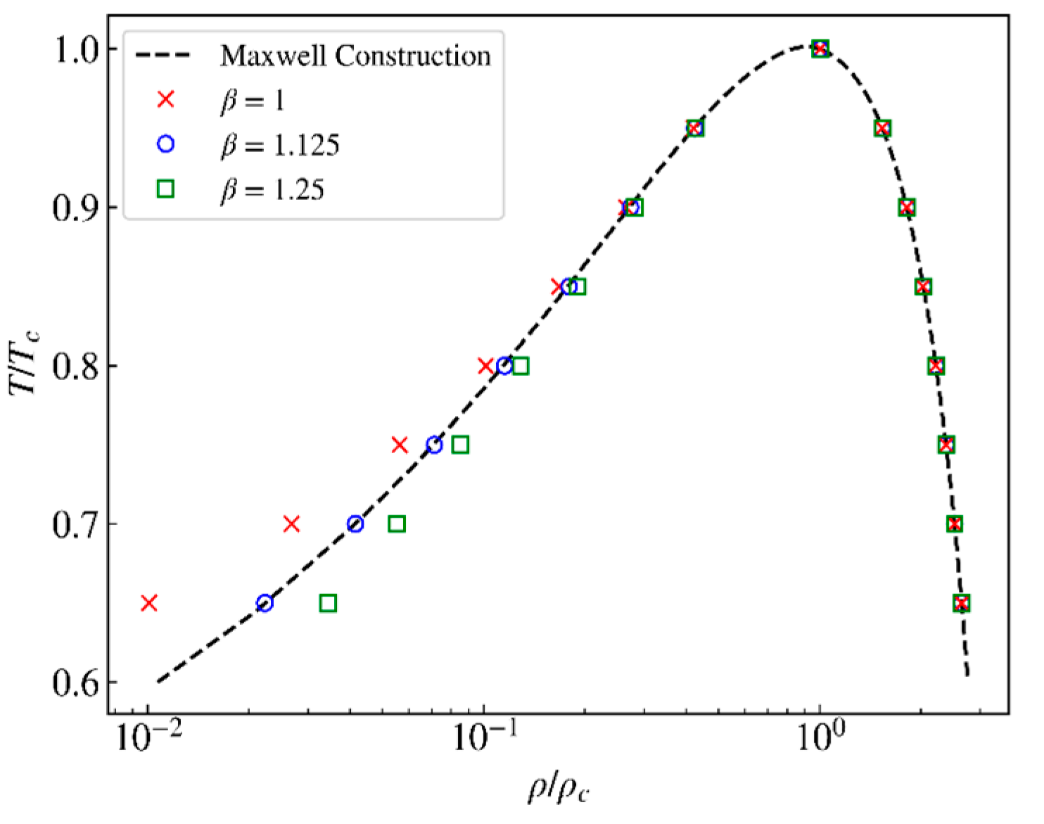
where W is the width of the phase interface, and is generally 2–5 grids. ρv and ρl are the gas and liquid densities of the Maxwell theory. In this method, the position of 50 ≤ y ≤150 is liquid phase and the other positions are gas phase. The gas–liquid interface is a straight line, and capillary pressure can be ignored [45]. We compare the gas–liquid coexistence density under β = 1, β = 1.125 and β = 1.25 and the Maxwell theory. As shown in Figure 2, when β = 1 (representing the original fluid-force format), it is observed that the gas–liquid density obtained from LBM simulation fails to match the gas–liquid density calculated directly using the RK EOS (solid line in Figure 2). However, by employing an improved fluid-force format and adjusting the coefficient β accordingly, we can achieve consistency between the gas–liquid density obtained from the LBM simulation and that derived from the RKEOS under specific temperature and pressure conditions. When β = 1.125, our LBM model basically shows agreement with the Maxwell theory, and β = 1.125 is therefore adopted.
Figure 2.
Comparison of gas–liquid coexistence density curves.
3.2. Verification of Interfacial Tension
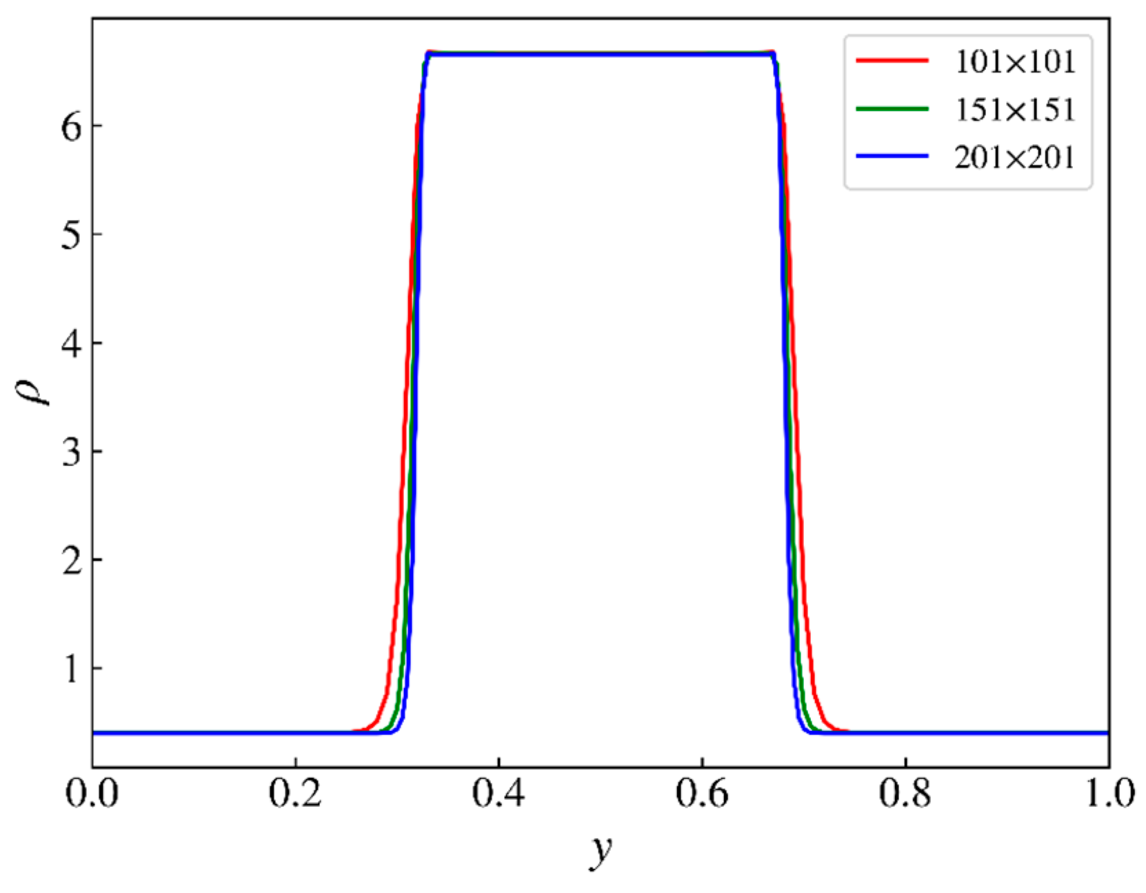
We calculate the interfacial tension by simulating the static circular droplet. Three different grid sizes (101 × 101, 151 × 151, 201 × 201) are constructed to simulate the density distribution of the static circular droplet and to test grid independence (this test is conducted to obtain a more accurate static interfacial tension.). The density initialization method proposed by Huang et al. [46] is adopted.
where R0 is the droplet initialization radius, and (x0, y0) is the initial center of the droplet. The simulation conditions are T = 0.8Tc, ρv = 0.342, and ρl = 6.60. The periodic boundary is used around the simulation, and the other parameters are consistent with those in Section 3.1. In order to facilitate comparison, the ratio of droplet diameter to grid size in different grids is kept consistent, and the simulation time step is selected to be 5000 to make the results stable. The simulation results are shown in Figure 3. The density distributions of the gas phase and liquid phase at the center line with different grid sizes are almost the same, indicating that simulation results are grid-independent, and the simulated results only have small deviations in the two-phase transition region. When the grid density exceeds 151 × 151, the simulation results of the density distribution are almost consistent, which meets the requirements of simulation accuracy. As a result, to save computational resources, the 151 × 151 grid space is selected for the simulation verification of interfacial tension.

Figure 3.
Density distribution of center line.
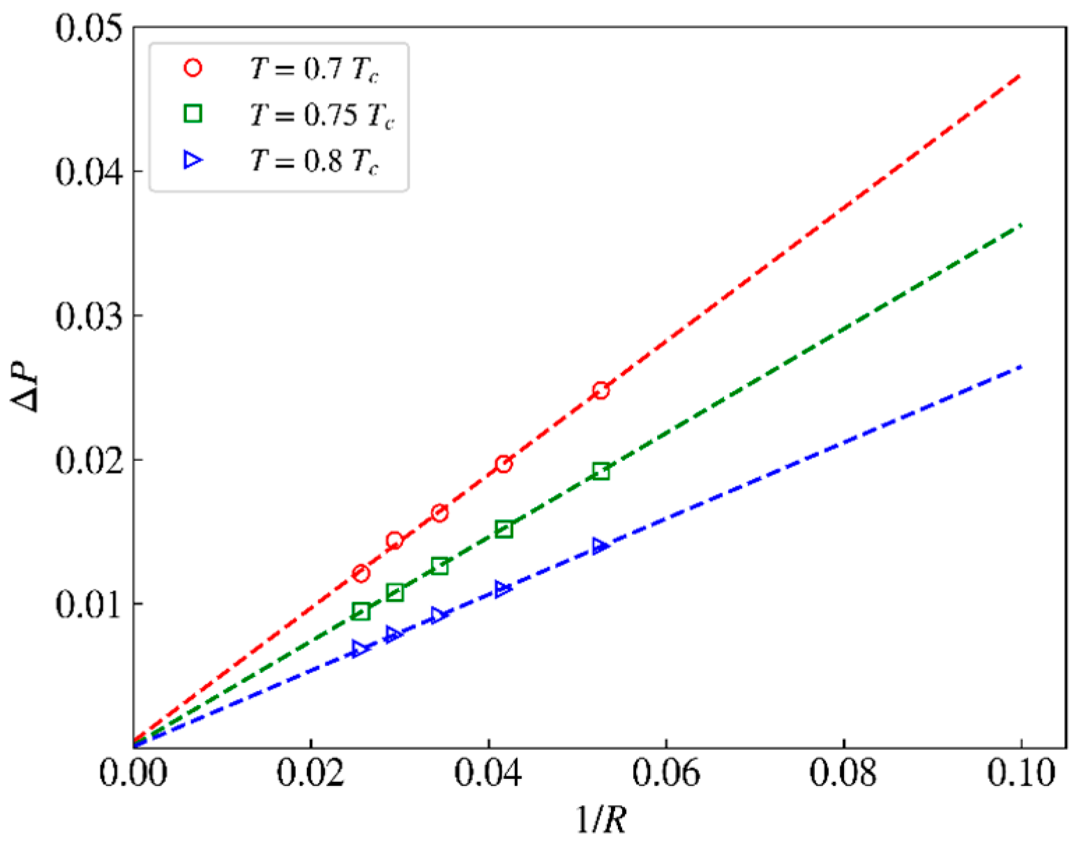
We further simulated the static behavior of the circular droplet at T = 0.7Tc, T = 0.75Tc and T = 0.8Tc. After the simulation reached equilibrium, the actual gas-hydraulic difference is calculated according to Equation (14). The interfacial tension is determined using the Young–Laplace equation, ∆P = Pint − Pout = σ/R [47]. In this study, the density of the gas–liquid interface is (ρv + ρl)/2, and the droplet diameter is determined based on this. By changing the droplet diameter, a series of pressure differences and its relationship with the droplet radius are obtained. As shown in Figure 4, the reciprocal of pressure and radius presents a good linear relationship (R2 is greater than 0.999). Through linear fitting, the tension values of the gas–liquid interface at different temperatures are 0.463, 0.361 and 0.264 lu, respectively (where lu stands for lattice unit).
Figure 4.
Verification of interfacial tension. (Dashed lines are fitting lines).
3.3. Verification of Static Contact Angle
In this work, the fluid–fluid force and fluid–solid wall force are considered, and a different contact between the droplet and wall are simulated on this basis. Chen et al. [42] gave a method for calculating the contact angles of the droplet on the wall:
where θ is contact angle, ξ1 is base length of the contact line between the droplet and solid wall, and ξ2 is height of the droplet. In order to verify different wetting angles, we established a grid area of 151 × 151, and set the periodic boundary in the x direction. y = 0 and y = Ny are taken as solid wall and are used as rebound boundaries [48]; simulated temperature T = 0.8Tc. Finally, the density initialization method proposed by Li et al. [49] is adopted as:
where R0 is the droplet initialization radius. In this paper, R0 = 15 lu, (x0, y0) = (75, 135) is set as the initial center of the droplet. The wetting angle can be simulated by varying the wall density ρw. The simulation results are shown in Figure 5.
Figure 5.
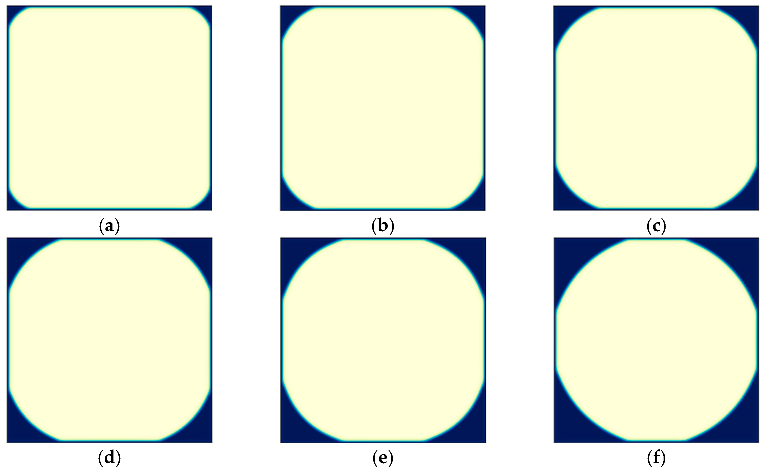
Simulation of different static contact angles, (a) θ = 0°; (b) θ = 25.8°; (c) θ = 50.0°; (d) θ = 83.7°; (e) θ = 132.4°; (f) θ = 180°. (Yellow is the gas phase and blue is the water phase).
3.4. Characteristics of Corner Liquid Retention
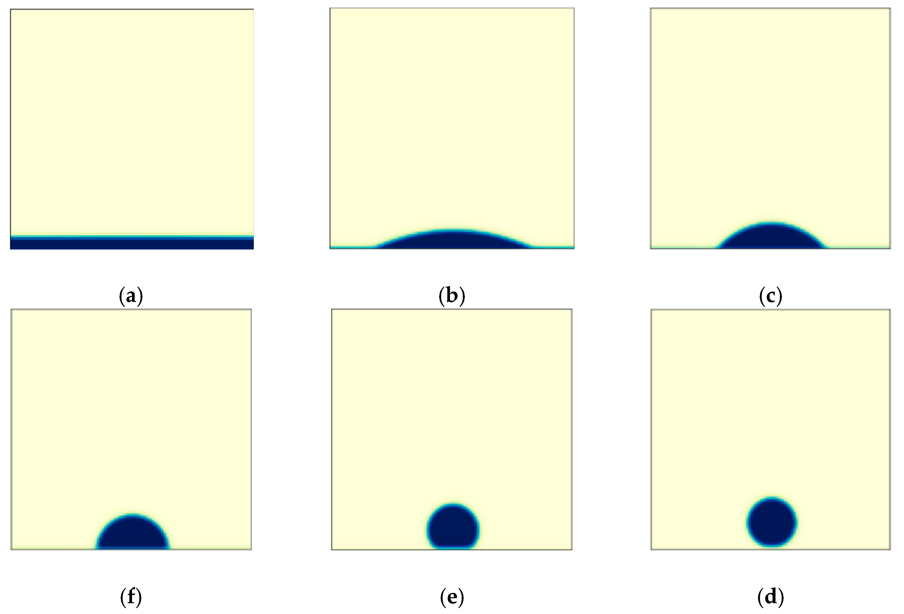
In square-section pores and throats, the liquid phase will remain at the corners of the pores and throats after gas displacement, whose retention characteristics (radius of curvature) have a certain effect on the snap-off in noncircular pores [50]. Therefore, to verify the accuracy of our model, we use pseudo-potential to simulate the relationship between the curvature radius of corner and liquid saturation. The conditions are as follows: a 151 × 151 grid space is established; temperature is set as T = 0.8Tc; solid walls and rebound boundary are adopted; the wetting angle is 0° and other parameters are consistent with Section 3.3. Based on Li et al. [49], we propose a new initialization density method to characterize the different radius of the curvature of the liquid phase in corner. The format is as follows:
where (x0, y0) = (75, 75) is the coordinate position of the initial center of the bubble, and R1 is the initial bubble radius, which ranges from 75 to 75√2 to represent different radius of curvature of the corner liquid (0 to 75). As shown in Figure 6, our model can capture the curvature radius of the liquid film and liquid phase at the corner of the wall. The characterization method of static liquid film thickness on the wall can be found in reference [51,52,53]. This paper mainly focuses on the relationship between the curvature diameters and saturation of liquid phase at the corner.
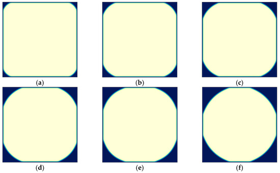
Figure 6.
Corner liquid retention characteristics, (a) Sl = 1.64%; (b) Sl = 4.3%; (c) Sl = 7.1%; (d) Sl = 9.8%; (e) Sl = 14.1%; (f) Sl = 18.6%. (Yellow is the gas phase and blue is the water phase).
By comparing the simulated results of the curvature radius and saturation of liquid phase at the corner with those proposed by Li et al. [54], the theoretical model can be simplified as follows, without considering the influence of wall–liquid film thickness:
where ε is the diameter of dimensionless curvature, ε = d/(L1 − 2h), L1 is the length of square pores, h is the thickness of liquid film, and d is the curvature diameter of corner liquid. In Figure 7, it can be seen that our simulation results are consistent with the theoretical results, indicating that our model can accurately evaluate the trend of occurrence of the liquid phase in the corner and determine the radius of the curvature of the liquid.
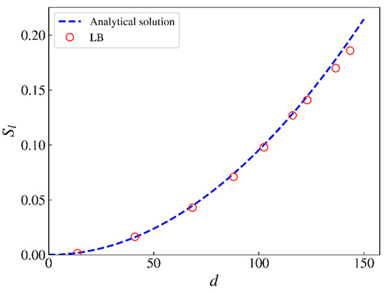
Figure 7.
The relationship between the curvature diameter of corner liquid and saturation.
3.5. Grid Independence Test
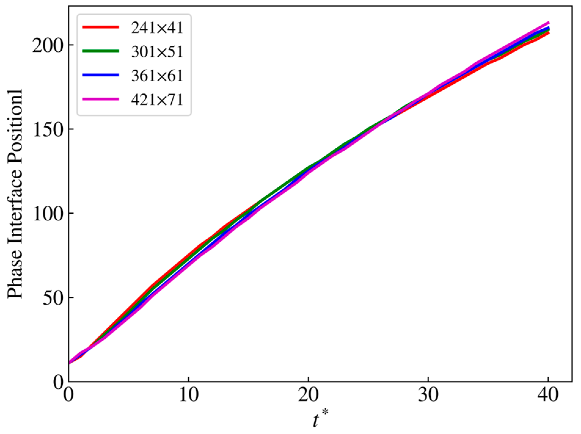
The grid independence test of the model is carried out through simulating the liquid phase displacement process in a single tube under different grid sizes (the vertex position of the curved liquid surface changed with time). To this end, four different grid sizes (241 × 41, 301 × 51, 361 × 61, 421 × 71) are established in this work. The bottom and top of the y-direction are used as solid boundaries with a non-slip rebound scheme. We set a 5 to 10 grid buffer area for the gas phase at the inlet and outlet; other places were set with the liquid phase. The external force flow at each node is added. We also applied a periodic boundary for the flow direction (x direction). When the liquid phase is displaced to the gas phase buffer area at the outlet, the liquid phase density is automatically replaced by the gas phase density at the next occurrence to realize the “disappearance” of the liquid phase in the buffer area, thus completing the displacement process. The simulation runs at T = 0.8Tc, ρv = 0.342 and ρl = 6.60 and the ratio of simulated displacement pressure and the ratio of simulated time step to the interval of sampling points remain constant, respectively. The simulation results are almost the same for different grid sizes in Figure 8. Therefore, the grid size of the simulation conditions is selected as 51 × 301 in the subsequent displacement simulations.
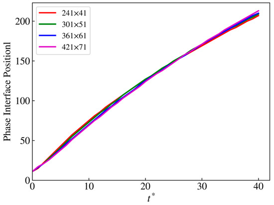
Figure 8.
Grid independence verification.
4. Discussion
4.1. Simulation of Snap-Off Phenomenon
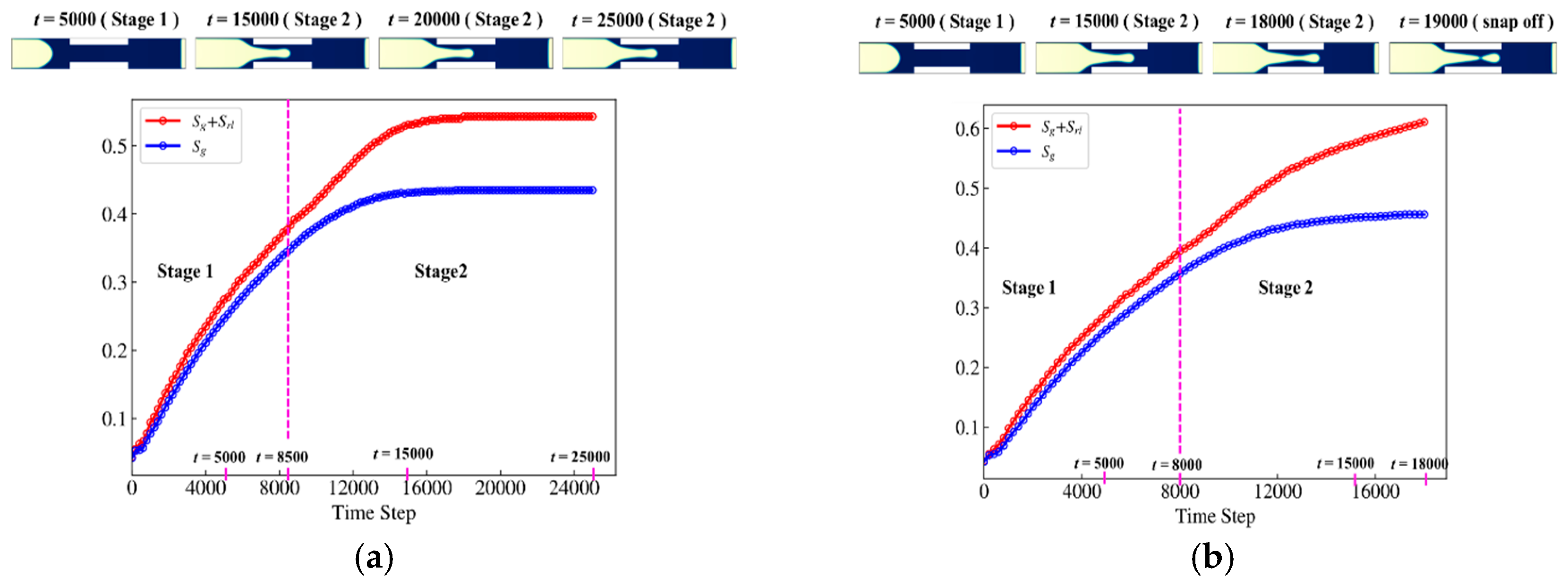
We establish a grid space of 301 × 51 and set a throat with a width of 30 lu (L* = 0.2, R* = 0.6) at 120 < x < 180 and 10 < y < 40. The boundary in the x direction is the same as the one in Section 3.5. The throat wall is set as solid wall with a rebound boundary at y = 0 and y = 50, and the contact angle is set as 0°. The simulation conditions are as follows: (1) The gas phase density ρv = 0.53 lu, the liquid phase density ρl = 6.08 lu, and the density ratio (ρr = 11.5) are close to the density ratio (ρr = 11) of water and methane at 15 MPa, 350 K from, the NIST chemical database. (2) The gas phase viscosity μv is 0.088 lu and the liquid viscosity μl is 1.013 lu. (3) The interfacial tension between the two phases is σ = 0.178 lu.
To express the displacement more clearly, we divide the whole process into three stages by time: (1) The gas phase displacement stage in the pores at the left end. (2) The displacement stage of the gas phase invasion of the throat. (3) The gas phase breaks through the throat and enters the displacement stage of the pores at the right end. We select gas phase saturation Sg, which is the ratio of the volume fraction of the gas phase to the volume fraction of the entire region. During the displacement, the retained liquid phase saturation Srl is used, which refers to the ratio of the liquid volume fraction within the boundary to the volume fraction of the whole region in the process of displacement. The vertex of the two-phase curved liquid surface is taken as the dividing line (vertical line), as parameters to quantitatively characterize the liquid phase changes. Since Sg + Srl is equivalent to the total area affected by gas flooding in the process of piston displacement with a flat interface in the petroleum field, we captured the changing rule of Sg and Sg + Srl over time and listed the density distribution of the two-phase fluid at a certain point in three stages (Figure 9). In the first stage (t < 9000), the gas phase is displaced in the pores at the left end. A relatively stable curved liquid surface is formed and Srl remains a low value during. In the second stage (9000 ≤ t ≤ 13,000), there is retained liquid at the corner of the pore and throat wall, and Srl increases gradually with the increase in simulated time step. In the third stage (t > 13,000), the gas phase broke through the throat and entered the pores at the right end. Due to the strong wettability of the wall, the gas phase could not contact the wall; a large amount of liquid phase was retained on the pore wall at the right end, which resulted in the Srl increasing rapidly. Finally, the retained wetting phase gradually flowed back into the throat over time, and finally formed the snap-off. In addition, the conditions used for the snap-off observed (R* = 0.6) do not satisfy the static criterion for the snap-off (R* ≤ 0.53). This is because the gas phase cannot create contact with the throat wall and the pore wall at the right end in the second and third stages. As a result, the radius of the leading edge after the gas phase that breaks through the throat is always smaller than the pore radius and the value of Cm is too large, which makes the prediction of the derived static criterion based on the angle flow conservative.
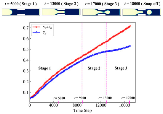
Figure 9.
Sg and Srl changes at different time steps. (Yellow is the gas phase and blue is the water phase).
We further calculate the changes in the Pc-neck and Pc-front values in the third stage, as shown in Figure 10. With the increase in time step, Pc-neck increases along with Srl; after the gas phase breaks through the throat, the curvature radius of the leading-edge increases, leading to the continuous reduction in Pc-front. Finally, Pc-neck > Pc-front causes the retained liquid phase to backflow and forms snap-off.
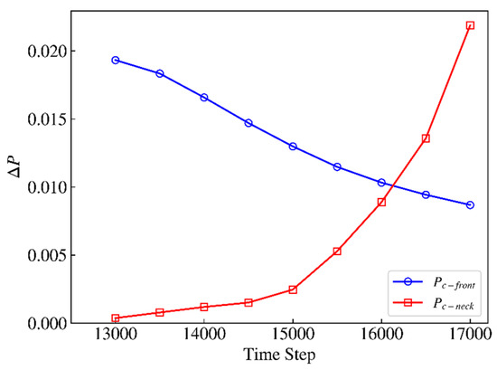
Figure 10.
Pc-neck and Pc-front changes at different time steps.
The above results show agreement with the previous static criteria for judging the occurrence of snap-off, which indicates that Roof et al.’s [6] snap-off mechanism based on unbalanced capillary pressure is also applicable in the mutant pore–throat system. Meanwhile, the above 2D simulation results are basically consistent with the experimental results of bubble snap-off in the 3D pore–throat structure by Wu et al. [15], indicating that our simulation results are still valid for the actual 3D situation. However, a large number of studies have shown that dynamic factors had a great impact on the phenomenon of snap-off [11], but the current theoretical models are all quasi-static geometric criteria and cannot consider the impact of dynamic factors. Therefore, the pseudo-potential model is adopted to evaluate the influence of capillary number Ca, L* and R* on phase interface snap-off in gas–liquid two-phase displacement using numerical simulation.
4.2. Influence of Cappillary Number Ca
Capillary number is an important parameter of two-phase flow; it is defined as the following:
where ρn,νn represent the density and kinematic viscosity of the non-wetting phase, respectively, which are the same as the density and kinematic viscosity of the gas phase in the simulation of this paper. uave is the average velocity of two-phase displacement [9].
The influence of the capillary number on the snap-off will be studied by changing the displacement pressure under the following conditions: (1) Establish a 300 × 51 grid space; (2) Set a throat with length of 100 lu and width of 30 lu (L* = 0.33, R* = 0.6) at the position of 100 < x < 200 and 10 < y < 40; (3) Ensure the displacement pressure is ∆P = 0.069; (4) The edge position of phase interface is captured every 500 time steps, and the average displacement velocity (uave = ∆s/∆t) can be obtained using the curve of the relation between the phase interface position and time. It should be pointed out that ∆s and ∆t represent the displacement and time before the occurrence of the snap-off. Figure 11a shows the variation rule of Sg and Sg + Srl over time in the two-phase displacement, when Ca = 4.8 × 10⁻³ and the density distribution of two-phase fluid is at a certain time in the three stages. Firstly, the simulation results in the first stage show agreement with those in Section 4.1. Secondly, when the gas phase enters the throat, the retained liquid phase always exists in the pore corner and throat wall, resulting in the increase in Srl. While there is small displacement pressure the gas phase cannot break through the throat, and the gas–liquid interface ultimately maintains the balance in the throat and does not extend. Srl remained unchanged (Srl = 0.11). The reason for the above phenomenon is that the capillary pressure at the gas–liquid interface and the force at the solid–liquid interface form large flow resistance, which is called the capillary “pinning” effect [55]. Therefore, the primary condition for the snap-off is that displacement pressure can overcome the capillary “pinning” effect and form effective displacement.

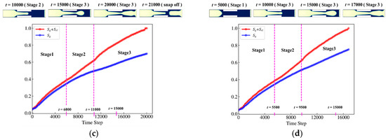
Figure 11.
Sg and Srl changes at different time steps, (a) Ca = 4.8 × 10⁻³; (b) Ca = 5.6 × 10⁻³; (c) Ca = 8.0 × 10⁻³; (d) Ca = 8.6 × 10⁻³. (Yellow is the gas phase and blue is the water phase).
We increased the displacement pressure to ∆p = 0.078, as shown in Figure 11b; this shows the variation rule of Sg and Sg + Srl with time and the density distribution of two-phase fluid at a certain time of the three stages when Ca = 5.6 × 10⁻³. The first stage is consistent with the simulation results above. After the gas phase enters the throat, the liquid phase remains in the pore corner and the throat wall, the liquid thickness on the throat wall presents an uneven distribution, and Srl increases gradually. With the increase in the time step, the retained liquid phase flows back and snaps off the phase interface in the second stage, which indicates that the snap-off can occur before the gas phase breaks through the throat in the non-gradual pore–throat system.
Keeping other conditions unchanged, we increased displacement pressure to ∆p = 0.105, as shown in Figure 11c. At this time, the capillary number (Ca = 8.0 × 10⁻³) is relatively large. Compared with the previous simulation results, the retained liquid phase saturation Srl on the throat wall in the second stage is small. With the time step increasing, the gas phase continues to flow forward and the snap-off does not occur until it breaks through the throat. When the gas phase reached the outlet, the retained liquid phase flows back and formed snap-off as the simulated time step continues to increase. In addition, the location of the snap-off moved to the outlet of the throat with the increase in capillary numbers, which shows agreement with the experimental results of Wei et al. [56], who used a 3D pore–throat structure to study bubble snap-off under different capillary numbers.
The displacement pressure is further increased to ∆p = 0.114 (Ca = 8.6 × 10⁻³), and the displacement pressure is large and Srl is small. As the time step increases, the gas phase breaks through the throat and eventually reaches the outlet. When the gas phase reaches the outlet, there is no snap-off with the increase in the simulated time step. It indicates that for a fixed pore–throat structure, there are critical capillary numbers. When the capillary numbers of the system are larger than the critical capillary numbers, the backflow of the retained liquid phase in the throat will be inhibited, so as to inhibit the occurrence of the snap-off.
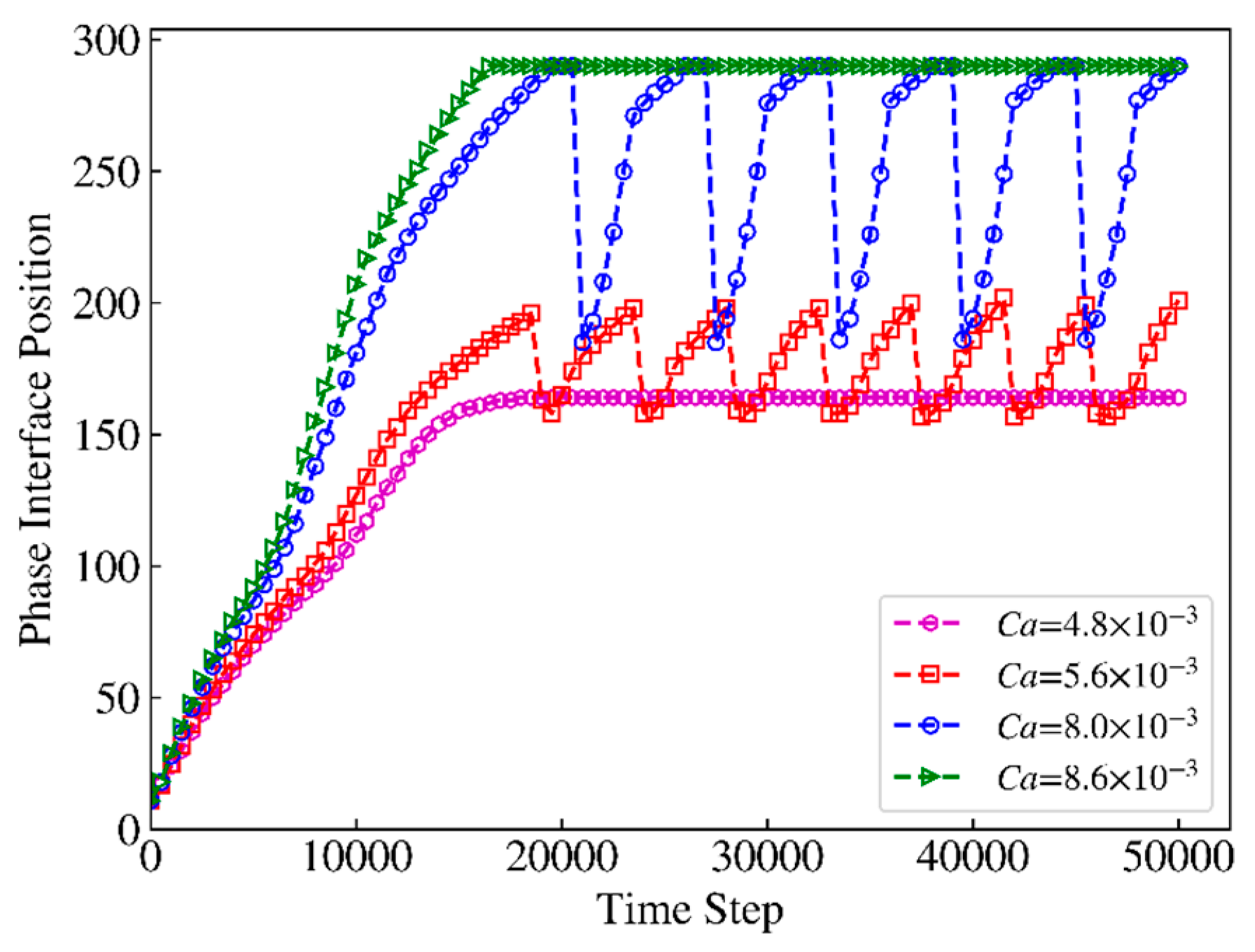
Figure 12 shows the changes in the leading-edge vertex positions of the phase interface over time under the above four conditions within 50,000 time-steps. After the occurrence of the snap-off, we took the peak of the curved liquid level in the throat as the actual phase interface position, so that when the phase interface position changed suddenly, it could be judged as the snap-off. We can see that when the gas phase is continuous, continuous snap-off can occur. The displacement and the location of the snap-off will hardly change each time, which is similar to the formation process of a droplet/bubble [57]. Meanwhile, for a specific pore–throat system, only when the capillary numbers meet a certain range will large capillary numbers inhibit the return of the retained liquid phase in the displacement and thus inhibit the occurrence of the snap-off, while small capillary numbers cannot overcome the capillary “pinning” effect to form effective displacement. Our simulation results are consistent with the conclusions obtained by Tsai et al. [9] in the study of bubble snap-off behavior under the pressure gradient at the gradual pore–throat.

Figure 12.
Change in phase interface position with time.
4.3. Influence of Pore–Throat Length Ratio
Pore–throat structure also has an important influence on the snap-off [9,10]. Therefore, we propose the pseudo-potential model to study the influence of different throat lengths on the snap-off. The conditions are as follows: (1) Establish a 301 × 51 grid space; (2) Set throats of the same width (R* = 0.6) but different lengths at the position 10 < y < 40. For different throat lengths, displacement pressure can better reflect the influence of dynamic factors on stuck fracture than capillary number. Therefore, we use displacement pressure to represent the influence of dynamic parameters instead of capillary numbers.
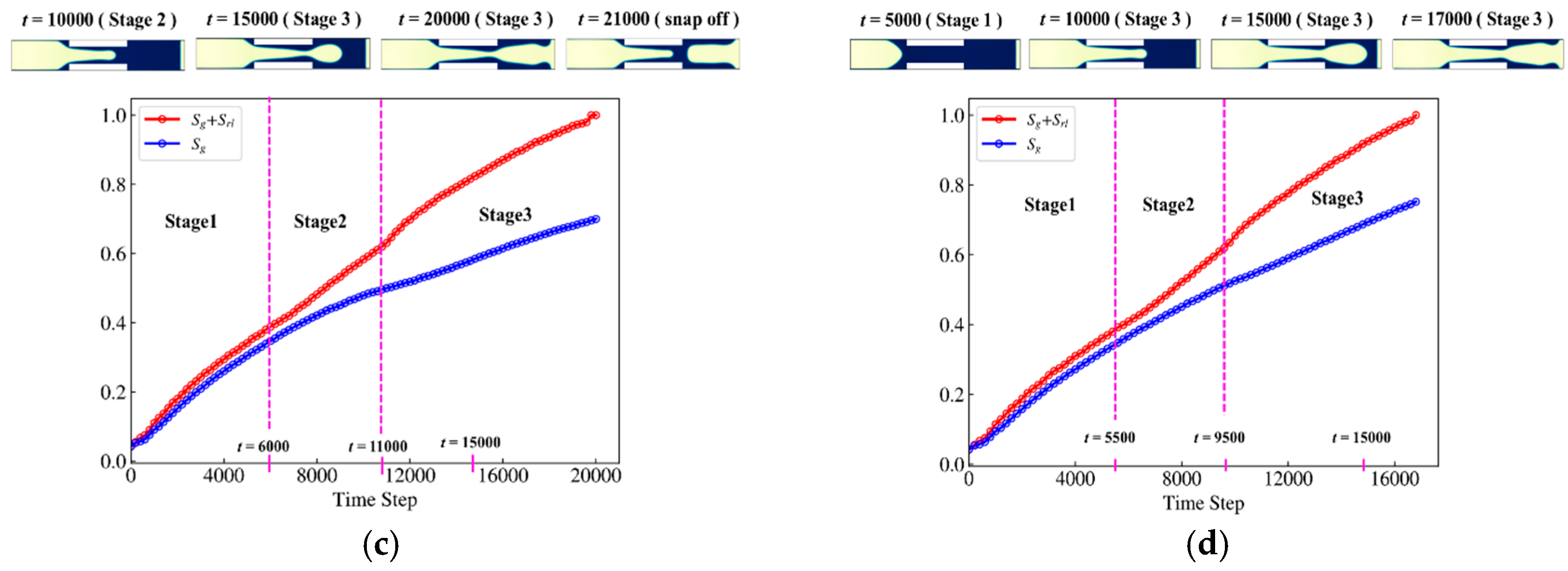
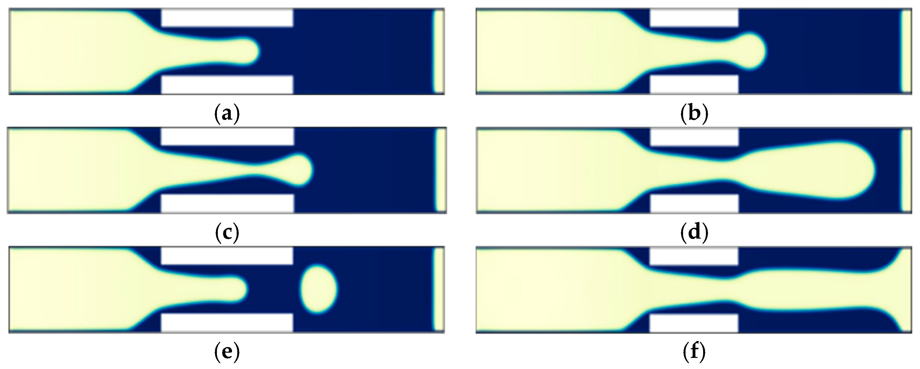
In the simulation, we determine the critical conditions for the snap-off by changing the displacement pressure (0.036 to 0.123) and L* (0.08 to 0.4). In this paper, the displacement effect of different pore–throat ratios are shown under two simulated conditions ∆p = 0.084 and L* = 0.3 as well as ∆p = 0.084 and L* = 0.2. As shown in Figure 13, at different time steps, with the decrease in throat length, the flow resistance decreases and the average two-phase displacement velocity increases, and the liquid saturation Srl retained in the pore corner and throat wall is low. However, it is worth noting that the pore–throat width ratio observed for the snap-off is inconsistent with that predicted using the static criterion (R* ≤ 0.53). This indicated that even if the pore–throat ratio of static criterion is not satisfied, a long enough throat length will promote the occurrence of the snap-off. Therefore, the pore–throat system with different throat lengths will present different flow states under the same displacement pressure.
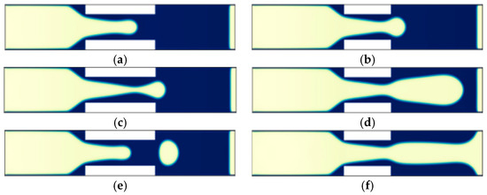
Figure 13.
Comparison of two-phase displacement processes, (a) t = 12,000, L* = 0.3; (b) t = 12,000, L* = 0.2; (c) t = 15,000, L* = 0.3; (d) t = 20,000, L* = 0.2; (e) t = 16,000, L* = 0.3; (f) t = 25,000, L* = 0.2. (Yellow is the gas phase and blue is the water phase).
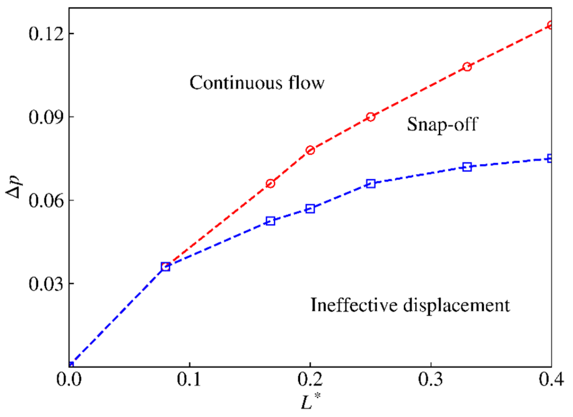
As the same time, we conduct a series of simulations to determine the conditions for the snap-off at different pore–throat length ratios and to finally obtain the critical displacement pressure for the snap-off, as shown in Figure 14. It can be seen that from the figure that for the pore–throat system with a fixed throat width, there is a critical length ratio (L* = 0.08), so that the change in displacement pressure will not cause the snap-off in gas–liquid two-phase displacement, which shows agreement with the conclusion proposed by Deng et al. [10] that the snap-off was inhibited in the short-wavelength gradual pore–throat. With the increase in throat length, a different displacement pressure difference will lead to three flow states: the snap-off, continuous flow and ineffective displacement in gas–liquid displacement. When displacement pressure is less than the lower limit of critical displacement pressure, the capillary “pinning” effect cannot be overcome and invalid displacement is formed. When the displacement pressure is greater than the upper limit of the critical displacement pressure, the gas phase will maintain a continuous flow state and inhibit the occurrence of the snap-off.
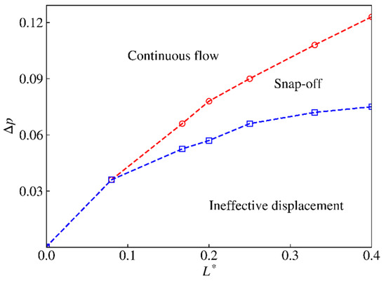
Figure 14.
The relationship between gas–liquid flow state and displacement pressure difference with different L*.
4.4. Influence of Pore–Throat Width Ratio
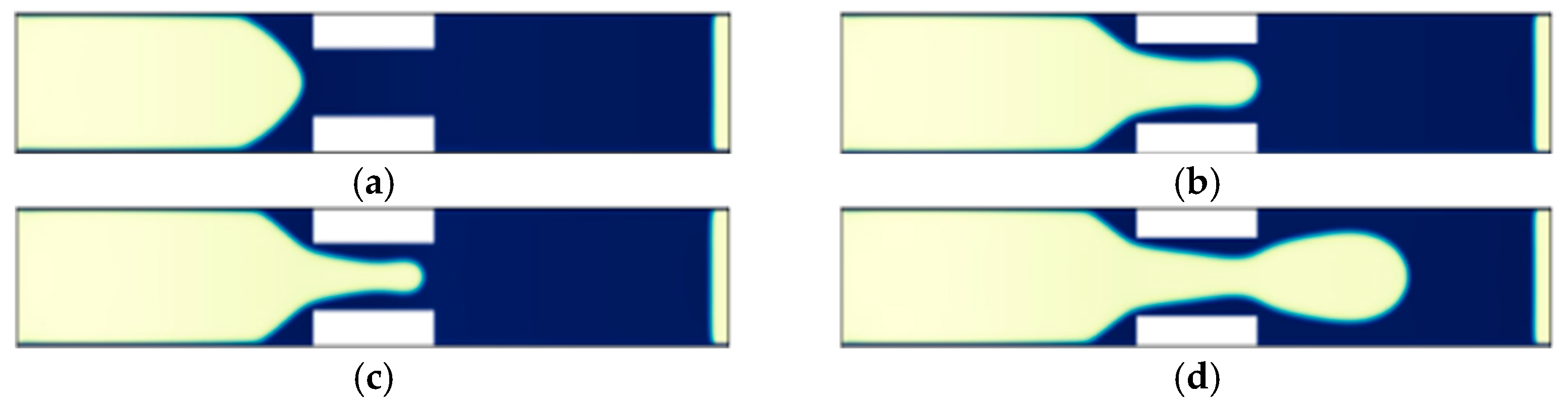
In this section, we study the influence of the throat width ratio on the snap-off by fixing L* and changing R*. The conditions are as follows: (1) Establish a 301 × 51 grid space; (2) Set the throat with a length of 50 lu (L* = 0.167) at 125 < x < 175; (3) Set other parameters in the same way as in Section 3.3. During the simulation, the critical condition is determined by changing the displacement pressure from 0.033 to 0.1 and the R* size from 0.52 to 0.68. Here, two groups of ∆p = 0.084, R* = 0.52 and ∆p = 0.084, R* = 0.6 are used as examples to show the effect of different pore–throat width ratios on flow state in gas–liquid two-phase displacement, as shown in Figure 15. It is found that with the decrease in throat width, the flow resistance increases significantly and the average two-phase displacement velocity decreases, while the liquid saturation Srl remains in the pore corner and the throat wall is higher. It is worth mentioning that R* = 0.52 meets the condition of static criterion (R* ≤ 0.53) and the phenomenon of the snap-off is observed, which verified the accuracy of our simulation results. In the case of R* = 0.6, there is no snap-off in the displacement, which also indicated that the increase in throat width will inhibit the snap-off.
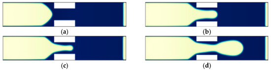
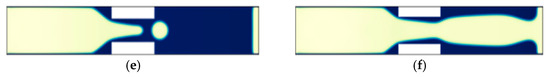
Figure 15.
Comparison of two-phase displacement processes, (a) t = 10,000, R* = 0.52; (b) t = 10,000, R* = 0.6; (c) t = 15,000, R* = 0.52; (d) t = 15,000, R* = 0.6; (e) t = 20,000, R* = 0.52; (f) t = 25,000, R* = 0.6. (Yellow is the gas phase and blue is the water phase).
We also simulated the effect of the pore–throat width ratio on the snap-off and the critical displacement pressure was obtained, as shown in Figure 16. Similar to Section 3.3, for a pore–throat system with a fixed throat length, the gas–liquid two-phase produce three types of flow states under different displacement pressures. With the increase in throat width, the range of the displacement pressure decreases gradually. When the width ratio increases to R* = 0.68, the change in the displacement pressure will not cause the snap-off in gas–liquid two-phase displacement. It is important to mention here that for R* = 0.52, which meets the condition for predicting the occurrence of the snap-off according to the static criterion, when the displacement pressure is greater than 0.1, the snap-off will not occur, indicating that the snap-off can be inhibited by a large displacement pressure, even if the static criterion is met. Meanwhile, based on Equation (1), the critical width ratio is predicted to be (R* = 0.53), which is 28.3% lower than the critical width ratio through simulation (R* = 0.68).
Figure 16.
The relationship between gas–liquid flow state and displacement pressure difference with different R*.
5. Conclusions
In this work, an improved pseudo-potential model and the improved fluid–fluid force scheme, regarding the original one component pseudo-potential-based LBM, are presented here. On this basis, the flow states of the gas–liquid two-phase in the pore–throat system under different displacement conditions are simulated. The following conclusions can be obtained:
- (1)
- The basic reason for the phase interface snap-off is that the liquid phase (wetting phase) retained in displacement gradually flows back over time due to unbalanced pore–throat capillary pressure. However, a large amount of retained liquid is observed in the pore corner and throat wall, which leads to the static criterion based on the assumption of the angular flow, which overestimates the radius of curvature of the bubbles on the right side of the throat and thus underestimates the conditions for the occurrence of the snap-off.
- (2)
- Revealing the influence of displacement pressure (capillary numbers) on gas–liquid two-phase displacement. In the non-gradual pore–throat system, only when displacement pressure is in a certain range, the snap-off will occur. If the upper limit of the capillary number is exceeded, even if the static condition is satisfied, the snap-off will be inhibited. Below this lower boundary, displacement cannot be completed. Meanwhile, the increase in capillary number makes the location of the snap-off move towards the outlet end of the throat.
- (3)
- Revealing the influence law of pore–throat length ratio on gas–liquid two-phase displacement. For the pore–throat system with a fixed width, a sufficiently long throat can promote the occurrence of the snap-off even if it does not meet the pore–throat width ratio (R* ≤ 0.53) for static criterion. The range of displacement pressure for the occurrence of the snap-off expends with the increase in throat length. In addition, there is a critical throat length, so that no matter how the displacement pressure changes, non-snap-off will happen in the throat. For the model in this paper, the critical pore–throat length ratio L* = 0.08.
- (4)
- Revealing the influence law of the pore–throat width ratio on gas–liquid two-phase displacement. For the pore–throat system with a fixed length, the larger the throat width, the smaller the displacement pressure range. There is a critical throat width so that no snap-off occurs in the throat, regardless of the displacement pressure. In this paper, the critical throat width ratio R* = 0.68. And it will underestimate by 28.3% if the static criterion is used to predict the condition of the model.
Author Contributions
Conceptualization, K.Z. and Y.J.; Methodology, K.Z., Y.J., T.Z. (Tao Zhang) and T.Z. (Tianyi Zhao); Software, Y.J.; Validation, T.Z. (Tianyi Zhao); Formal analysis, K.Z.; Investigation, T.Z. (Tianyi Zhao); Data curation, T.Z. (Tao Zhang). All authors have read and agreed to the published version of the manuscript.
Funding
This research was funded by [State Key Laboratory of Shale Oil and Gas Enrichment Mechanisms and Efficient Development] grant number [G5800-20-ZS-KFZY006] and [33550000-21-ZC0613-0015].
Data Availability Statement
Data are contained within the article.
Conflicts of Interest
T.Z. (Tao Zhang) was employed by Shaanxi Yanchang Petroleum (Group) Co., Ltd. The remaining authors declare that the research was conducted in the absence of any commercial or financial relationships that could be construed as a potential conflict of interest. The authors declare that this study received funding from [State Key Laboratory of Shale Oil and Gas Enrichment Mechanisms and Efficient Development]. The funder was not involved in the study design, collection, analysis, interpretation of data, the writing of this article or the decision to submit it for publication.
References
- Yun, W.; Kovscek, A.R. Microvisual investigation of polymer retention on the homogeneous pore network of a micromodel. J. Pet. Sci. Eng. 2015, 128, 115–127. [Google Scholar] [CrossRef]
- Liu, Z.; Zhuang, Z.; Meng, Q.; Zhan, S.; Huang, K.-C. Problems and challenges of mechanics in shale gas efficient exploitation. Chin. J. Theor. Appl. Mech. 2017, 49, 507–516. [Google Scholar]
- Yuan, S.; Wang, Q.; Li, J.; Han, H. Technology progress and prospects of enhanced oil recovery by gas injection. Acta Pet. Sincia 2020, 41, 1623–1632. [Google Scholar]
- Gao, Y.; Zhao, M.; Wang, J.; Zong, C. Performance and gas breakthrough during CO2 immiscible flooding in ultra-low permeability reservoirs. Pet. Explor. Dev. 2014, 41, 79–85. [Google Scholar] [CrossRef]
- Kong, D.; Gao, Y.; Sarma, H.; Li, Y. Experimental investigation of immiscible water-alternating-gas injection in ultra-high water-cut stage reservoir. Adv. Geo-Energy Res. 2021, 5, 139–152. [Google Scholar] [CrossRef]
- Roof, J.G. Snap-off of oil droplets in water-wet pores. Soc. Pet. Eng. J. 1970, 10, 85–90. [Google Scholar] [CrossRef]
- Gauglitz, P.A.; St Laurent, C.M.; Radke, C.J. Experimental determination of gas-bubble breakup in a constricted cylindrical capillary. Ind. Eng. Chem. Res. 1988, 27, 1282–1291. [Google Scholar] [CrossRef]
- Ransohoff, T.C.; Gauglitz, P.A.; Radke, C.J. Snap-off of gas bubbles in smoothly constricted noncircular capillaries. AIChE J. 1987, 33, 753–765. [Google Scholar] [CrossRef]
- Tsai, T.M.; Miksis, M.J. Dynamics of a drop in a constricted capillary tube. J. Fluid Mech. 2016, 274, 197–217. [Google Scholar] [CrossRef]
- Deng, W.; Cardenas, M.B.; Bennett, P.C. Extended Roof snap-off for a continuous nonwetting fluid and an example case for supercritical CO2. Adv. Water Resour. 2014, 64, 34–46. [Google Scholar] [CrossRef]
- Deng, W.; Balhoff, M.; Cardenas, M.B. Influence of dynamic factors on nonwetting fluid snap-off in pores. Water Resour. Res. 2015, 51, 9182–9189. [Google Scholar] [CrossRef]
- Tian, J.; Kang, Y.; Xi, Z.; Jia, N.; You, L.; Luo, P. Real-time visualization and investigation of dynamic gas snap-off mechanisms in 2-D micro channels. Fuel 2020, 279, 118232. [Google Scholar] [CrossRef]
- Cha, L.M.; Xie, C.Y.; Feng, Q.H.; Balhoff, M. Geometric Criteria for the Snap-Off of a Non-Wetting Droplet in Pore-Throat Channels with Rectangular Cross-Sections. Water Resour. Res. 2021, 57, e2020WR029476. [Google Scholar] [CrossRef]
- Tetteh, J.T.; Cudjoe, S.E.; Aryana, S.A.; Ghahfarokhi, R.B. Investigation into fluid-fluid interaction phenomena during low salinity waterflooding using a reservoir-on-a-chip microfluidic model. J. Pet. Sci. Eng. 2021, 196, 108074. [Google Scholar] [CrossRef]
- Wu, Y.; Fang, S.; Dai, C.; Sun, Y.; Fang, J.; Liu, Y.; He, L. Investigation on bubble snap-off in 3-D pore-throat micro-structures. J. Ind. Eng. Chem. 2017, 54, 69–74. [Google Scholar] [CrossRef]
- Xiong, Q.R.; Baychev, T.G.; Jivkov, A.P. Review of pore network modelling of porous media: Experimental characterisations, network constructions and applications to reactive transport. J. Contam. Hydrol. 2016, 192, 101–117. [Google Scholar] [CrossRef]
- Monaghan, J.J. Smoothed particle hydrodynamics. Annu. Rev. Astron. Astrophys. 1992, 30, 543–574. [Google Scholar] [CrossRef]
- Armstrong, R.T.; Berg, S.; Dinariev, O.; Evseev, N.; Klemin, D.; Koroteev, D.; Safonov, S. Modeling of pore-scale two-phase phenomena using density functional hydrodynamics. Transp. Porous Media 2016, 112, 577–607. [Google Scholar] [CrossRef]
- Raeini, A.Q.; Blunt, M.J.; Bijeljic, B. Modelling two-phase flow in porous media at the pore scale using the volume-of-fluid method. J. Comput. Phys. 2012, 231, 5653–5668. [Google Scholar] [CrossRef]
- Chen, S.Y.; Doolen, G.D. Lattice Boltzmann method for fluid flows. Annu. Rev. Fluid Mech. 1998, 30, 329–364. [Google Scholar] [CrossRef]
- Raeini, A.Q.; Bijeljic, B.; Blunt, M.J. Numerical modelling of sub-pore scale events in two-phase flow through porous media. Transp. Porous Media 2014, 101, 191–213. [Google Scholar] [CrossRef]
- Starnoni, M.; Pokrajac, D. Numerical study of the effects of contact angle and viscosity ratio on the dynamics of snap-off through porous media. Adv. Water Resour. 2018, 111, 70–85. [Google Scholar] [CrossRef]
- Zhang, C.; Yuan, Z.; Matsushita, S.; Xiao, F.; Suekane, T. Interpreting dynamics of snap-off in a constricted capillary from the energy dissipation principle. Phys. Fluids 2021, 33, 032112. [Google Scholar] [CrossRef]
- Zhang, M.; Sun, J.; Chen, W. An interface tracking method of coupled Youngs-VOF and level set based on geometric reconstruction. Chin. J. Theor. Appl. Mech. 2019, 51, 775–786. [Google Scholar]
- Li, Q.; Yu, Y.; Tang, S. Multiphase lattice Boltzmann method and its applications in phase-change heat transfer. Chin. Sci. Bull. 2020, 65, 1677–1693. [Google Scholar] [CrossRef]
- Zang, C.; Qin, L. Lattice Boltzmann simulation of immiscible displacement in the complex micro-channel. Acta Phys. Sin. 2017, 66, 154–162. [Google Scholar]
- Rothman, D.H.; Keller, J.M. Immiscible cellular-automaton fluids. J. Stat. Phys. 1988, 52, 1119–1127. [Google Scholar] [CrossRef]
- Shan, X.W.; Chen, H.D. Lattice Boltzmann model for simulating flows with multiple phases and components. Phys. Rev. E 1993, 47, 1815. [Google Scholar] [CrossRef]
- Swift, M.R.; Osborn, W.R.; Yeomans, J.M. Lattice Boltzmann simulation of nonideal fluids. Phys. Rev. Lett. 1995, 75, 830. [Google Scholar] [CrossRef] [PubMed]
- He, X.Y.; Shan, X.W.; Doolen, G.D. Discrete Boltzmann equation model for nonideal gases. Phys. Rev. E 1998, 57, R13. [Google Scholar] [CrossRef]
- Zhang, L.; Kang, L.; Jing, W.; Guo, Y.; Sun, H.; Yang, Y.; Yao, J. Flow behavior analysis of oil-water two-phase flow in pore throat doublet model. J. China Univ. Pet. (Ed. Nat. Sci.) 2020, 44, 89–93. [Google Scholar]
- Zhao, Y.; Liu, X.; Zhang, L.; Tang, H.; Xiong, Y.; Guo, J.; Shan, B. Laws of gas and water flow and mechanism of reservoir drying in tight sandstone gas reservoirs. Nat. Gas Ind. B 2020, 40, 70–79. [Google Scholar] [CrossRef]
- Alpak, F.O.; Zacharoudiou, I.; Berg, S.; Dietderich, J.; Saxena, N. Direct simulation of pore-scale two-phase visco-capillary flow on large digital rock images using a phase-field lattice Boltzmann method on general-purpose graphics processing units. Comput. Geosci. 2019, 23, 849–880. [Google Scholar] [CrossRef]
- Wei, B.; Hou, J.; Sukop, M.C.; Du, Q.; Wang, H. Flow behaviors of emulsions in constricted capillaries: A Lattice Boltzmann simulation study. Chem. Eng. Sci. 2020, 227, 115925. [Google Scholar] [CrossRef]
- Zhang, T.; Javadpour, F.; Li, J.; Zhao, Y.; Zhang, L.; Li, X. Pore-Scale Perspective of Gas/Water Two-Phase Flow in Shale. SPE J. 2021, 26, 828–846. [Google Scholar] [CrossRef]
- Bhatnagar, P.L.; Gross, E.P. Krook MA model for collision processes in gases, I. Small amplitude processes in charged and neutral one-component systems. Phys. Rev. 1954, 94, 511. [Google Scholar] [CrossRef]
- Qian, Y.H.; d’Humières, D.; Lallemand, P. Lattice BGK models for Navier-Stokes equation. EPL (Europhys. Lett.) 1992, 17, 479. [Google Scholar] [CrossRef]
- Yuan, P.; Schaefer, L. Equations of state in a lattice Boltzmann model. Phys. Fluids 2006, 18, 042101. [Google Scholar] [CrossRef]
- Huang, H.B.; Li, Z.T.; Liu, S.S.; Lu, X. Shan-and-Chen-type multiphase lattice Boltzmann study of viscous coupling effects for two-phase flow in porous media. Int. J. Numer. Methods Fluids 2009, 61, 341–354. [Google Scholar] [CrossRef]
- Huang, H.B.; Sukop, M.; Lu, X.Y. Multiphase Lattice Boltzmann Methods: Theory and Application; Wiley: New York, NY, USA, 2015. [Google Scholar]
- Gong, S.; Cheng, P. Numerical investigation of droplet motion and coalescence by an improved lattice Boltzmann model for phase transitions and multiphase flows. Comput. Fluids 2012, 53, 93–104. [Google Scholar] [CrossRef]
- Chen, L.; Kang, Q.; Mu, Y.; He, Y.-L.; Tao, W.-Q. A critical review of the pseudopotential multiphase lattice Boltzmann model: Methods and applications. Int. J. Heat Mass Transf. 2014, 76, 210–236. [Google Scholar] [CrossRef]
- Mukherjee, A.; Basu, D.N.; Mondal, P.K. Algorithmic augmentation in the pseudopotential-based lattice Boltzmann method for simulating the pool boiling phenomenon with high-density ratio. Phys. Rev. E 2021, 103, 053302. [Google Scholar] [CrossRef]
- Kupershtokh, A.L.; Medvedev, D.A.; Karpov, D.I. On equations of state in a lattice Boltzmann method. Comput. Math. Appl. 2009, 58, 965–974. [Google Scholar] [CrossRef]
- Huang, J.; Yin, X.; Barrufet, M.; Killough, J. Lattice Boltzmann simulation of phase equilibrium of methane in nanopores under effects of adsorption. Chem. Eng. J. 2021, 419, 129625. [Google Scholar] [CrossRef]
- Huang, H.B.; Krafczyk, M.; Lu, X.Y. Forcing term in single-phase and Shan-Chen-type multiphase lattice Boltzmann models. Phys. Rev. E Stat. Nonlin. Soft Matter Phys. 2011, 84, 046710. [Google Scholar] [CrossRef]
- Shi, D.; Wang, Z.; Zhang, A. A novel lattice boltzmann model simulating gas-liquid two-phase flow. Chin. J. Theor. Appl. Mech. 2014, 46, 224–233. [Google Scholar]
- Hu, W.; Liu, G.; Yan, S.; Fan, Y. Pore-Scale lattice Boltzmann modeling of soil water Distribution. Chin. J. Theor. Appl. Mech. 2021, 53, 568–579. [Google Scholar]
- Li, Q.; Luo, K.H.; Kang, Q.J.; Chen, Q. Contact angles in the pseudopotential lattice Boltzmann modeling of wetting. Phys. Rev. E 2014, 90, 053301. [Google Scholar] [CrossRef]
- Kovscek, A.R.; Radke, C.J. Gas bubble snap-off under pressure-driven flow in constricted noncircular capillaries. Colloids Surf. A Physicochem. Eng. Asp. 1996, 117, 55–76. [Google Scholar] [CrossRef]
- Li, J.; Li, X.; Wang, X.; Li, Y.; Wu, K.; Shi, J.; Yang, L.; Feng, D.; Zhang, T.; Yu, P. Water distribution characteristic and effect on methane adsorption capacity in shale clay. Int. J. Coal Geol. 2016, 159, 135–154. [Google Scholar] [CrossRef]
- Li, J.; Li, X.; Wu, K.; Feng, D.; Zhang, T.; Zhang, Y. Thickness and stability of water film confined inside nanoslits and nanocapillaries of shale and clay. Int. J. Coal Geol. 2017, 179, 253–268. [Google Scholar] [CrossRef]
- Li, J.; Li, X.; Wu, K.; Wang, X.; Shi, J.; Yang, L.; Zhang, H.; Sun, Z.; Wang, R.; Feng, D. Water sorption and distribution characteristics in clay and shale: Effect of surface force. Energy Fuels 2016, 30, 8863–8874. [Google Scholar] [CrossRef]
- Li, J.; Chen, Z.X.; Wu, K.L.; Zhang, T.; Zhang, R.; Xu, J.; Li, R.; Qu, S.; Shi, J.; Li, X. Effect of water saturation on gas slippage in circular and angular pores. AIChE J. 2018, 64, 3529–3541. [Google Scholar] [CrossRef]
- Fuquan, S.; Xiao, H.; Genmin, Z.; Weiyao, Z. The characteristics of water flow displaced by gas in nano arrays. Chin. J. Theor. Appl. Mech. 2018, 50, 553–560. [Google Scholar]
- Wei, B.; Wang, Y.Y.; Wen, Y.B.; Zhu, W. Bubble breakup dynamics and flow behaviors of a surface-functionalized nanocellulose based nanofluid stabilized foam in constricted microfluidic devices. J. Ind. Eng. Chem. 2018, 68, 24–32. [Google Scholar] [CrossRef]
- Si, T. Dynamic behavior of droplet formation in dripping mode of capillary flow focusing. Capillarity 2021, 4, 45–49. [Google Scholar] [CrossRef]


Disclaimer/Publisher’s Note: The statements, opinions and data contained in all publications are solely those of the individual author(s) and contributor(s) and not of MDPI and/or the editor(s). MDPI and/or the editor(s) disclaim responsibility for any injury to people or property resulting from any ideas, methods, instructions or products referred to in the content. |
© 2024 by the authors. Licensee MDPI, Basel, Switzerland. This article is an open access article distributed under the terms and conditions of the Creative Commons Attribution (CC BY) license (https://creativecommons.org/licenses/by/4.0/).