Article

Heat Transfer Estimation in Flow Boiling of R134a within Microfin Tubes: Development of Explainable Machine Learning-Based Pipelines

by
Shayan Milani
,
Keivan Ardam
,
Farzad Dadras Javan
,
Behzad Najafi
*,
Andrea Lucchini
,
Igor Matteo Carraretto
and
Luigi Pietro Maria Colombo
Dipartimento di Energia, Politecnico di Milano, Via Lambruschini 4, 20156 Milano, Italy
*
Author to whom correspondence should be addressed.
Energies 2024, 17(16), 4074; https://doi.org/10.3390/en17164074
Submission received: 13 June 2024 / Revised: 2 August 2024 / Accepted: 13 August 2024 / Published: 16 August 2024
(This article belongs to the Section J1: Heat and Mass Transfer)

Abstract

:
The present study is focused on identifying the most suitable sequence of machine learning-based models and the most promising set of input variables aiming at the estimation of heat transfer in evaporating R134a flows in microfin tubes. Utilizing the available experimental data, dimensionless features representing the evaporation phenomena are first generated and are provided to a machine learning-based model. Feature selection and algorithm optimization procedures are then performed. It is shown that the implemented feature selection method determines only six dimensionless parameters ( S u l : liquid Suratman number, B o : boiling number, F r g : gas Froude number, R e l : liquid Reynolds number, B d : Bond number, and e / D : fin height to tube’s inner diameter ratio) as the most effective input features, which reduces the model’s complexity and facilitates the interpretation of governing physical phenomena. Furthermore, the proposed optimized sequence of machine learning algorithms (providing a mean absolute relative difference (MARD) of 8.84% on the test set) outperforms the most accurate available empirical model (with an MARD of 19.7% on the test set) by a large margin, demonstrating the efficacy of the proposed methodology.

1. Introduction

Thermal management of components is a challenging task in many industries such as high-precision manufacturing; miniaturized heating, ventilation, and air conditioning (HVAC) systems; heat pumps; and heat dissipation in electric vehicles. The HVAC sector has long transitioned from using smooth tubes to microfin tubes in condensers and evaporators. In horizontal ducts, the swirled fins help the fluid reach the tube’s upper part, and the dry-out phenomenon occurs at qualities greater than 0.9, which widely compensates for the drawbacks of a larger pressure drop per unit length and higher costs. Evaporation inside a horizontal smooth tube is characterized by a sequence of different flow regimes which changes as the quality shifts from x = 0 to x = 1 and the mass flux changes and is affected by the liquid’s and the vapor’s thermal properties. This complexity makes employing the analytical approach extremely challenging. On the other hand, a numerical approach is still not feasible due to the unsteady behavior of the interfaces and the small size of the droplets, which require a mesh with very small elements. This results in long calculation times, with no guarantee of the solution’s reliability. Therefore, up to now, the only viable approach for investigating evaporation has been the experimental one, yielding a set of empirical correlations. Moreover, from a manufacturing point of view, it is feasible to produce microfins with various shapes, patterns, and details (Figure 1 represents geometries and examples of microfin tubes). That adds further complexity to the topic of evaporation inside tubes.
One of the earliest studies on evaporation in microfin tubes was conducted by Thome et al. [1]. In this research, the authors considered the combined effects of nucleate and convective boiling of R134a and R123. Their heat transfer correlation was the first general method that could be applied to any two-dimensional microfin geometry and fluid of interest. Around the same time, Cavallini et al. [2] were working on an empirical model, taking into account both the nucleate and the forced convection boiling for different surface geometries. Additionally, they managed to extend Thome et al.’s correlation [1] to zeotropic mixtures of R407C and R32/R134a. A promising agreement between the experimental values and the models’ estimations was observed.
Yun et al. [3] worked only on distinguishing the dimensionless parameters and the physical phenomena suitable to represent the enhanced heat transfer performance of microfin tubes compared to the smooth ones without employing the corresponding flow patterns. The authors proposed that the enhancement in the case of nucleate boiling depends on the surface tension and the turbulence effects, whereas in the case of convective boiling, it is correlated with a modified Reynolds number. Moreover, they also proposed the ratio of liquid film thickness over fin height as an influential factor. Accordingly, they implemented their proposed parameters into the basic form of evaporation heat transfer correlation for smooth tubes, thus obtaining a relatively good estimation performance over the available database.
Chamra and Mago [4] collected an experimental database, which included pure refrigerants and mixtures flowing within microfin tubes. The authors proposed a semi-empirical formulation for the evaporation heat transfer prediction achieving MARD in the range of 10–25%. More recently, Rollmann and Spindler [5] collected an extensive database of 1600 points to formulate a correlation to predict the Nusselt number of the evaporating flow. The latter, which included a wide range of saturation temperatures, heat fluxes, mass fluxes, and vapor qualities, was demonstrated to predict 94.2% of data points within the ±30% MRD range. Moreover, in another recent study, Han et al. [6] analyzed the flow boiling heat transfer characteristics of R161/oil mixtures. The authors based their model on the local properties of the refrigerant/oil mixture and the geometry structure of the microfin tube. The latter model was able to predict the experimental data points with an accuracy between −15 and +20%. A little while later, Mehendale [7] used a database of 2622 points to develop a new correlation for the flow boiling Nusselt number in horizontal microfin tubes. The author selected 38 relevant dimensionless parameters and then applied a multivariable regression analysis in order to find the ones with the highest relevance to flow boiling. The correlation obtained by this method was able to predict 71.5–80.5% of the data points within ±30%, with a mean absolute deviation of 21.5 to 25.2%. Most recently, a new correlation to predict the heat transfer coefficient for large temperature glide working fluids was proposed in a work conducted by Dai et. al. [8], and a mean absolute deviation of 16.9% was obtained. Besides the superposition methods discussed previously, there are alternative ones, such as those relying on energy dissipation [9]. In a work performed by Pysz et al. [10], flow boiling of R1233zd(E) in a 3 mm vertical stainless steel tube was presented at moderate and high saturation temperatures. The in-house model, a modified version of it, and some well-known correlations were compared, and it was shown that the modified model outperforms the others with an MAPE of 23.17% for R1233zd(E).

1.1. Artificial Intelligence and Machine Learning Models

Artificial intelligence (AI) is a field of computer science that enables machines with computing capabilities (intelligent systems) to make rational decisions based on specific inputs. It has found applications in many industries, from automation processes to decision making in critical areas. Machine learning (ML) is a subset of AI, which leverages statistical learning techniques and extracts patterns from raw data to make a subjective decision without being explicitly programmed [11]. Considering their higher accuracy, machine learning models have been employed in several studies for simulating the multiphase flow phenomena and analysis of thermal systems; control and modeling of evaporative condensers [12]; modeling, control, and performance assessment of heat exchangers [13,14,15]; pressure drop prediction of non-Newtonian flows [16]; performance assessment of fin-tube evaporators [17]; and multiphase flows’ pressure drop prediction [18,19]. Among all the available ML algorithms, the artificial neural network (ANN) has attracted the most interest among scholars [20,21].
The two early studies by Thibault and Grandjean [22] and Jambunathan et al. [23] took the initial step in applying ANN in heat transfer analysis. Chen et al. [24] proposed an overlapped type of local neural network to improve the accuracy of the heat transfer coefficient estimation of the super-critical carbon dioxide. The study conducted by Pacheco-Vega et al. [25] used a limited experimental dataset. The limited size of this dataset showed the capability of ANN in heat rate estimation of a fin-tube refrigeration heat exchanger. Scalbarian et al. [26] employed ANN-based methods for the prediction of flow boiling heat transfer of pure refrigerants and compared the results with the empirical models in the literature to show that ANN outperforms these models. The same authors in another study extended the use of the ANN model to mixture boiling heat transfer estimation [27]. Zhao and Zhang [28] modeled a fin-tube air-cooled condenser with an ANN. In the next step, the authors compared the outcome with a validated first-principle model and reached an impressive standard deviation of 1.9%.
In many studies, authors comprehensively modeled a heat exchanger with an ANN. An example is the work carried out by Xie et al. [29] that applied an ANN-based model for heat transfer analysis of two different types of shell-and-tube heat exchangers, one with segmental baffles and the other with continuous helical baffles. The authors investigated different network configurations to find the one with the most promising prediction performance. The obtained result showed the superiority of the ANN over other correlations which are used for the prediction. Only recently, ML models other than ANNs have also been used for multiphase flow heat transfer estimation. Zhou et al. [30] developed machine learning-based models for predicting condensation heat transfer coefficients in mini/micro-channels. The authors carried out a parametric optimization procedure for a few ML algorithms and demonstrated that utilizing ANN and XGBoost algorithms leads to the highest performance. Following the study, Hughes et al. [31] employed three ML models of artificial neural networks, support vector regression, and random forest in heat transfer estimation in condensing flows. The study revealed that the random forest model exhibits more remarkable performance in comparison with the other two algorithms, resulting in an absolute average deviation value of close to 4%.
In an attempt to predict the boiling and condensation heat transfer performance of R134a in mini-channels with serrated fins, Zhu et al. [32] utilized ANN and experimental data obtained from two mini-channels. Elements such as channel dimensions, fluid properties, operational conditions, and derived dimensionless parameters were considered as input for the ML pipelines (a set of preprocessing steps and a sequence of machine learning algorithms (with specific hyperparameters )). The proposed ANN models estimated the heat transfer coefficient during boiling exhibiting a mean absolute relative deviation (MARD) of 11.41%. Moradkhani et al. [33] employed a dataset of 1035 samples from diverse studies to assess the performance of multilayer perceptron (MLP), Gaussian process regression (GPR), and radial basis function (RBF) machine learning algorithms in predicting the boiling heat transfer coefficient (HTC) in smooth, helically coiled tubes. The evaluation of these algorithms revealed that the tested dataset yielded an average absolute relative error (AARE) of 5.93%. Despite this, the study notably omitted the evaluation of alternative machine learning algorithms and the optimization of hyperparameters, which could potentially provide better insight and predictive accuracy. Furthermore, the research sought to identify significant input features by examining their Pearson correlation with the Nusselt number. It was found that input parameters with high correlations did not necessarily enhance the predictive capability of the models. However, the investigation would not systematically analyze the performance of individual input features and their combinations in making accurate predictions. In their work on predicting heat transfer coefficients during flow boiling in mini/micro-channels, Ari Bard et al. [34] utilized a dataset of 16,653 points and a variety of different machine learning models including random forests and support vector machines. It was shown that the support vector machine model obtained a mean absolute percentage error (MAPE) of 11.3%. Regarding the feature selection, some of the common libraries of feature reduction were deployed (e.g., principal component analysis (PCA), Boruta, recursive partitioning, etc).
While there isexisting literature on the application of artificial neural networks (ANN) and other machine learning (ML) models for heat transfer estimation in multiphase flows, to the best of the authors’ knowledge, no prior study has specifically delved into optimizing ML pipelines (including algorithms and tuning parameters). Specifically, there is a scarcity of studies that systematically address the refinement of algorithms and tuning parameters to enhance performance. Additionally, more effort is required regarding an explainable systematic feature selection approach to identify the most promising set of features by including combinations of features in prediction systematically. This would not only reduce model complexity but also facilitate a clearer physical interpretation of the results obtained. Encouraged by the mentioned research gap, the present study develops an optimized machine learning-based pipeline for heat transfer estimation of evaporating R134a flow in microfin tubes with various geometrical configurations.

1.2. The Contributions of The Present Study

The current work employs a set of experiments on R314a flow undergoing the evaporation process in microfin tubes under various operating conditions resulting in various datasets of the heat transfer coefficients and the corresponding operating conditions. Next, widely adopted empirical correlations for heat transfer estimation of two-phase flows are collected from the literature and are applied to the available experimental dataset to obtain the corresponding accuracy. Afterward, several ML-based pipelines are constructed, taking the dimensionless parameters inspired by the thermo-fluid dynamics of the evaporation process as the input features and the two-phase Nusselt number as the estimation target. A feature selection step provides the most promising features among a pool of features while improving/maintaining the accuracy, resulting in reduced computational costs and better understanding of the governing physical phenomena. Next, the optimization step provides the pipeline that yields the highest prediction accuracy, and the corresponding performance on the test set is obtained. Ultimately, another in-house algorithm, referred to as forward feature combination, is implemented, taking the optimal pipeline and the selected features as inputs and demonstrating the contribution of each feature to the overall achieved accuracy. Given that the number of implemented features denotes the complexity of the model, the forward feature combination provides a trade-off between the complexity of the model and the obtained accuracy.
Hence, the contributions of the current study can be outlined as follows:
  • Utilizing the experimental dataset on R134a flow under diverse operating conditions undergoing the evaporation process within microfin tubes.
  • Gathering widely adopted empirical correlations for heat transfer estimation of two-phase flows from the literature and applying them to the available experimental dataset to obtain their performance.
  • Developing various ML pipelines utilizing a range of ML algorithms including extra trees regressor and assessing their performance.
  • Providing a feature selection procedure to identify the most promising set of features by employing various combinations of features systematically in the prediction of the target and assessing their performance, leading to a notable reduction in the number of features, reducing model complexity, and facilitating physical interpretation of the results.
  • Utilizing a genetic algorithm-based pipeline optimization tool, with a focus on identifying the most suitable algorithm from a broad array of machine learning solutions, refining the tuning parameters, and their sequence in the pipeline.
  • Employing an in-house algorithm (forward feature combination), taking the optimal pipeline and the selected features as inputs, and demonstrating the contribution of each feature to the overall achieved accuracy, providing a trade-off between the complexity of the model and the obtained accuracy.

2. Experimental Activity and the Employed Dataset

The experimental facility, from which the dataset was obtained, was designed to run experiments in the most common operating conditions of HVAC devices that, for a given fluid, are uniquely identified by the refrigerant’s mass flux, the refrigerant’s inlet quality in the test section, the mean quality in the test section, and the quality change in the test section. In order to take into account the two heat transfer mechanisms (convective evaporation and nucleate boiling), the experiments were designed in a way that a wide range of operating conditions were possible. The tests were performed employing three configurations of microfin tubes, presented in Table 1. The experimental apparatus is depicted in Figure 2, while its schematic is in Figure 3, which illustrates the position and the type of installed measurement devices and a detailed drawing of the test section, which is provided to demonstrate its main features, as shown in Figure 4. The main geometrical features of the microfin tubes used for the experiments are listed in Table 1, while Figure 1 provides the corresponding graphical representation, comparing them with the smooth tube, which is the reference geometry for the performance comparison.

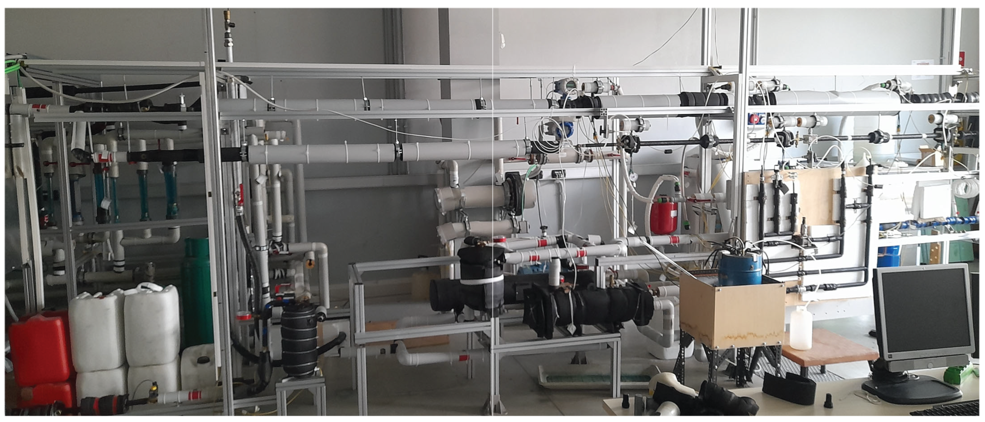
2.1. The Laboratory Setup

As illustrated in Figure 4, the layout of the experiment consists of three circuits: the refrigerant loop, the demineralized water loop, and the water/ethylene glycol (30% volume concentration) mixture loop. These circuits interact with one another and transfer thermal power to set the desired operating condition (in the test section).
Figure 2. The employed laboratory setup utilized for conducting the experiments.
Energies 17 04074 g002
The refrigerant circuit (red line) provides the R134a flow in the desired inlet quality, mass flow rate, and flow regime to the test section. An electric heater supplies thermal power to evaporate the refrigerant and set the required quality of the two-phase flow. Passing through the calming section, the refrigerant then reaches a fully developed flow regime. Finally, the thermal power exchange with the demineralized water circuit in the test section completes the evaporation process and enables obtaining the desired outlet quality of the two-phase flow. On the other hand, the glycol mixture circuit, by exchanging heat with the refrigerant in the condenser and subcooler, sets the desired pressure (and hence the corresponding saturation temperature) in the refrigerant loop. These three circuits are equipped with measurement and control units to monitor and regulate the pressure, the temperature, and the flow rate at different sections of the loop. The detailed description of the utilized experimental setup, the employed measurement procedures, the performed uncertainty analysis, and the selected operating conditions are provided in [35,36].
Figure 3. A schematic representation of the laboratory setup utilized for conducting the experiments.
Energies 17 04074 g003

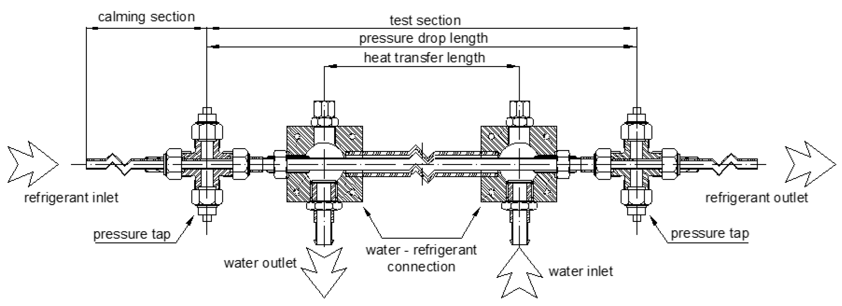
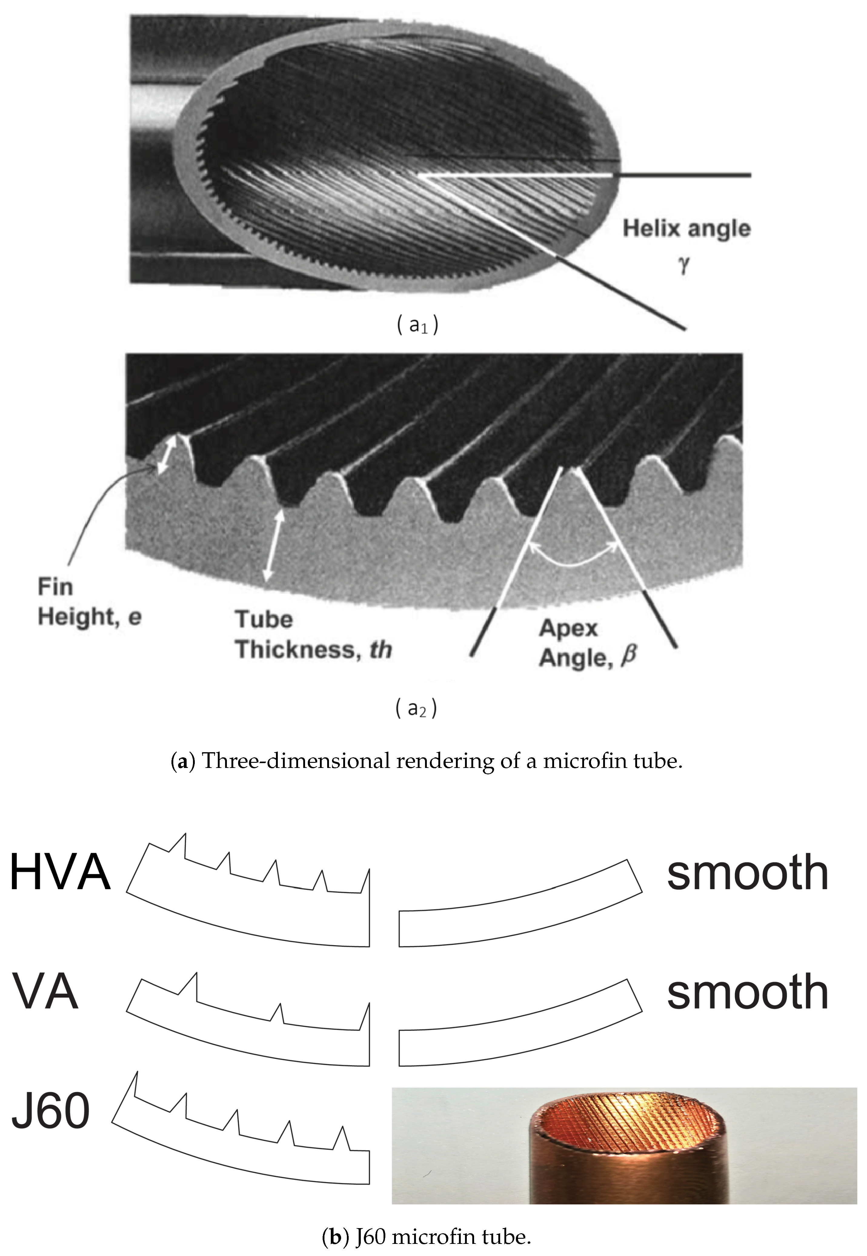
2.2. The Test Section

A tube-in-tube heat exchanger forms the test section. The demineralized water runs in the outer tube, and the refrigerant flows through the inner one, which is equipped with three different configurations of microfins (Table 1). To make sure that there is no thermal leakage to the surrounding environment, the outer tube is insulated with a 10 cm thick layer of rubber foam shell. Specific measurement units are utilized for monitoring the temperature in the test section.
Figure 4. A schematic representation of the test section in the experimental setup.
Energies 17 04074 g004

Temperature Measurement

The temperature of the refrigerant at the inlet and the outlet sections is measured by two K-type thermocouples [37] in the wells provided at the center line of the refrigerant passage. To obtain the wall temperature of the outer side of the microfin tube, three thermocouples are inserted into the wall in three different positions: at the bottom, the side, and the top. The resulting average is then computed as the representative of the wall temperature.

2.3. Experiments

The duration of each test is 3 min, and a data acquisition unit (DAU), which samples the reading at 1 Hz frequency, builds up the dataset. The uncertainties associated with each measurement unit are shown in Table 2.
Three variables, including the refrigerant mass flux, the mean quality in the test section, and the quality change through the test section, were varied in the experiments. The temperature fluctuations, after reaching steady state, require variables adjustment to make sure that the temperature is kept at a constant level. Therefore, the measurements were carried out (after every variable adjustment) 10–13 times, depending on the observed fluctuations. The ranges in the variation of variables are provided in Table 3.

3. Dimensionless Numbers of Phase-Changing Flow

Several physical phenomena coexist during the evaporation process. Consequently, a combination of operating and geometrical parameters that govern these physical phenomena affects the evaporation process. The dimensionless groups, according to the Buckingham theorem, are the most general way to represent the influence of all of the physical phenomena into a quantitative representation and hence are currently adopted in the literature for the development of empirical correlations. In the present study, these dimensionless groups are used as features for constructing machine learning-based pipelines. Table 4 summarizes the utilized dimensionless parameters along with the corresponding mathematical formulations.
The characteristic quantities reported in the definitions of some dimensionless groups may change from author to author; attention has to be paid to properly implement each model. For that reason, in Table 4, the characteristic length is generically named Dh, while in the correlations reported in Table 5, the quantity selected by the authors is reported. In the proposed correlations, all the authors selected the inner diameter at the fin root as the characteristic length. Furthermore, there are two different characteristic velocities, one for the vapor phase and the other for the liquid phase, which refer to the mass flux of each phase such that the former is G x ρ v and the latter is G ( 1 x ) ρ l . They represent the bulk velocity of each phase as if it flows alone in the tube.
In addition to the mentioned ones, three other dimensionless groups that represent the geometrical characteristics of the microfin tubes, including the number of fins (n), the fin height to tube’s inner diameter ratio ( e / D ), and the geometry enhancement factor ( R x ), are also adopted as features.
R x = 2 e n 1 sin γ 2 π D cos γ 2 + 1 1 cos β
Table 4. Dimensionless numbers [38].
 Dimensionless Number FormulationNo.
Nusselt number N u = h D h k l (2)
Reynolds number R e l = G ( 1 x ) D h μ l ,   R e g = G x D h μ g (3)
Weber number W e l = [ G ( 1 x ) ] 2 D h ρ l σ ,   W e g = ( G x ) 2 D h ρ g σ (4)
Froude number F r l = [ G ( 1 x ) ] 2 g D h ρ l 2 ,   F r g = ( G x ) 2 g D h ρ g 2 (5)
Prandtl number P r l = μ l c p l k l ,   P r g = μ g c p g k g (6)
Boiling number B o = q G h l g (7)
Jakob number J a = c p T s a t T w a l l h l g (8)
Bond number B d = g ( ρ l ρ g ) D h 2 σ (9)
Convection number C o = 1 1 x 0.8 ρ g ρ l 0.5 (10)
Kapitza number K a = μ 4 g ρ l σ 3 (11)
Galileo number G a = ρ l g ( ρ l ρ g ) D h 3 μ l 2 (12)
Suratman number S u l = σ ρ l D h μ l 2 = R e l 2 W e l ,   S u g = σ ρ g D h μ g 2 = R e g 2 W e g (13)
Lockhart–Martinelli parameter [39] X t t = 1 x x 0.9 ρ g ρ l 0.5 μ l μ g 0.1 (14)
Dimensionless vapor velocity [40] J g = G x g D ρ g ρ l ρ g (15)
Reduced pressure p r e = p s a t p c (16)
Table 5. The evaporation heat transfer correlations for microfin tubes.
Author(s) EquationNo.
Mehendale 1 [7] Π 34 = q D i n t μ l h l g , Π 35 = q h l g 1.5 ( ρ l ρ g )
Π 1 = 2 e n π D i n t 1 c o s 2 ( β ) + t a n 2 ( γ 2 ) t a n ( γ 2 ) + 1
Π 26 = D i n t G l 2 ρ g σ , Π 7 = 1 x x
Π 15 = 4.364 i f R e l 2300 ( f l / 8 ) ( R e l 1000 ) P r l 1 + 12.7 ( f l / 8 ) 0.5 ( P r l 2 3 1 ) i f R e l > 3000 C u b i c i n t e r p o l a t i o n i f 2300 < R e l < 3000
Π 24 = ρ g σ D i n t μ g 2 , Π 21 = G t p 2 D i n t ρ l σ , Π 6 = ρ l ρ g ρ l , Π 8 = M M H 2
Π 33 = g ( ρ l ρ g ) e D i n t σ n
N u = 0.03771 . Π 34 1.459 . Π 35 1.139 . Π 1 0.6214 . Π 26 0.2249 . Π 7 0.2253 . Π 15 0.1209
. Π 24 0.6149 . Π 21 0.04878 . Π 6 1.661 . Π 8 0.04224 . Π 33 0.1121
(17)
Han et al. [6] N u = h D i n t k f , h = F h r , l + S h r , n b
F = 1 + 7196.741 B o 1.16 + 1.5135 1 X t t 0.86 , S = 1 1 + 2.703 F 1.94 R e f 1.17
R e f = G x 1 D i n t μ f
h r , n b = 55 P r 0.12 ( log ( P r ) ) 0.55 M 0.5 q 1000 0.67
h r , l = E R B h l
h l = 0.023 R e f 0.8 P r f 0.4 k f D i n t
E R B = 1 + 2.64 R e f 0.036 e D i n t 0.212 p D i n t 0.21 β 90 0.29 P r f 0.024 7 1 7
(18)
 Rollmann and Spindler [5] N u = h D i n t k f = 1.2 3.7 P r f 2 + 0.71 R e f o 2 3 ln ( B o ) + 12.17 x 3.7 P r f 2 + 0.71
R e f o = G t p D i n t μ f
(19)
Chamra and Mago [4] h = 1.516 h p b X t t 1.161 0.01 D i n t 1.764 +
+ h l ϕ R x 2.622 B d F r g o 0.2158 0.01 D i n t 0.5927 100 G t p 0.0582
h p b = 55 P r 0.12 ( log ( P r ) ) 0.55 M 0.5 q 1000 0.67
F r g o = G t p 2 ρ g 2 g D i n t , B d = g ρ f π e D i n t 8 σ n
h l = 0.023 R e f 0.8 P r f 0.4 k f D i n t
R e f = G t p x 1 D i n t μ f
ϕ = 1 x + 2.63 x ρ f ρ g 0.5 0.8
N u = h D i n t k f
(20)
Yun et al. [3] h = h l 0.009622 B o 0.1106 P s a t D i n t σ 0.3814 + 7.685 1 X t t 0.51 G t p e μ f 0.736 ×
× R e f 0.2045 P r f 0.7452 D i n t 1 ϵ 4 e 0.1302
h l = 0.023 R e f 0.8 P r f 0.4 k f D i n t
R e f = G t p x 1 D i n t μ f
N u = h D i n t k f
(21)
Cavallini et al. [2] h = h n b + h c v
h n b = 55 P r 0.12 ( log ( P r ) ) 0.55 M 0.5 q 1000 0.67 × 1.36 X t t 0.36 0.01 D i n t 0.38
h c v = k f D i n t 0.023 R e f o 0.8 P r f 1 3 ϕ R x 2.14 B d F r g o 0.15 0.01 D i n t 0.59 100 G t p 0.36
ϕ = 1 x + 2.63 x ρ f ρ g 0.5 0.8 , R e f o = G t p D i n t μ f
B d = g ρ f π e D i n t 8 σ n , F r g o = G t p 2 ρ g 2 g D i n t
N u = h D i n t k f
(22)
Thome et al. [1] h = E m f h n b 3 + E R B h c v 3 1 3
h c v = 0.0133 R e f 0.69 P r f 0.4 k f δ
h n b = 55 P r 0.12 ( log ( P r ) ) 0.55 M 0.5 q 1000 0.67
δ = D i n t 1 ϵ 4 , R e f = G t p x 1 D i n t μ f
E m f = 1.89 G t p 500 2 3.7 G t p 500 + 3.02
E R B = 1 + 2.64 R e f 0.036 e D i n t 0.212 p D i n t 0.21 β 90 0.29 P r f 0.024 7 1 7
N u = h D i n t k f
(23)
1 fl is the Darcy liquid flow friction factor.

4. Empirical and Semi-Empirical Correlations

Many studies in the literature have been focused on heat transfer estimation of evaporating flows within horizontal tubes. Several attempts to provide a general representation of the heat transfer performance of microfin tubes have been made in spite of the large variety of microfin geometries. The evaporation models proposed by Mehendale [7], Han et al. [6], Rollmann and Spindler [5], Chamra and Mago [4], Yun et al. [3], Cavallini et al. [2], and Thome et al. [1] are among the most widely used correlations that have also demonstrated a relatively promising performance on the experimental dataset of the present study. Table 5 reports the mathematical expression of these models.

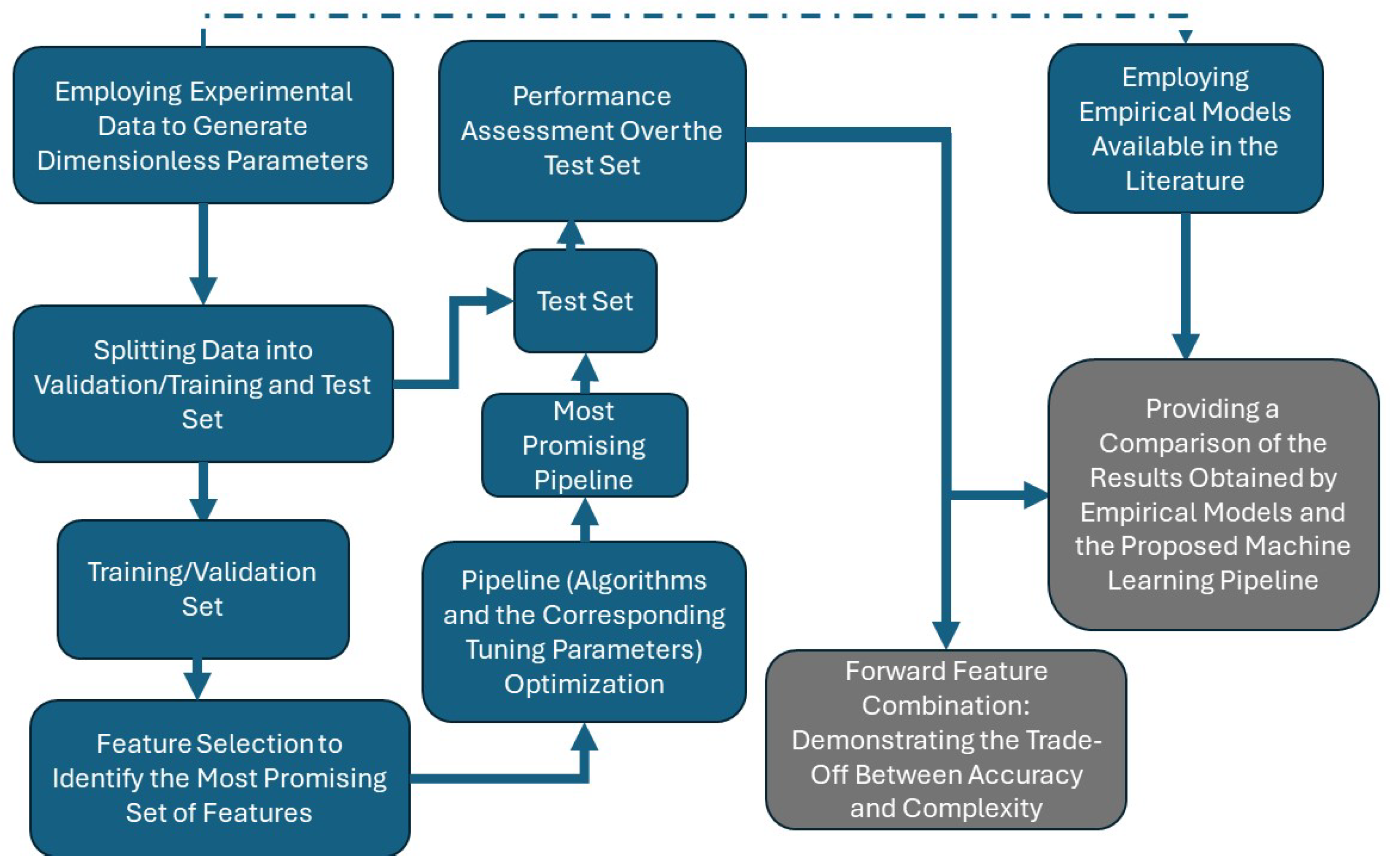
5. Methodology and Implemented Pipelines

Machine learning (ML) refers to automated statistical learning algorithms, which can predict the desired target employing a dataset. In an ML problem, an automated algorithm goes through an input dataset, searching for a mathematical relationship, to relate some features of the dataset to a specific target (supervised learning). The ML algorithms (models) differ from one another in the mathematical function that describes the relationship between the input features and the desired output. The advantages and drawbacks of each ML model come from the properties of this underlying function. The application of ML models is case-dependent, meaning that based on the characteristics of the dataset, some models perform better than others. Moreover, it is also possible to employ the advantages of several ML models by placing them after one another in a certain sequence. These sequential ML models are named pipelines.
In this research work, the physics of evaporation is first studied to find the most diverse set of dimensionless parameters, which describe different aspects of the evaporation process. Then, these parameters are utilized as input features for training several ML models and pipelines to estimate the Nu number, which is proportional, as expressed in Equation (2), to the heat transfer coefficient (the characteristic length is constant while the temperature oscillation recorded during the experiments was not larger than 2 K, which makes the variations of the liquid thermal conductivity smaller than 1%) as the target parameter representing the heat transfer behavior. There are two reasons behind this specific choice of the target parameter. Firstly, since the geometry of the microfins dominantly controls the evaporation process and the flow pattern formations, their geometry effect needs to be considered in the target. Secondly, as the liquid phase is in direct contact with the tube’s surface to prevent dry-out, its thermal conductivity also remarkably affects the evaporation process. Therefore, the Nusselt number, encompassing the hydraulic diameter and the liquid thermal conductivity, well represents these two effects.
The aim is to find the pipeline, together with the most promising set of features, which provides the most promising performance among all of the available pipelines. Therefore, this study has two levels of investigation: firstly, defining the feature set, which has the most effective relevance to the target of the estimation, and secondly, defining the pipeline, which provides the highest accuracy.
The dataset requires special treatment before being utilized for training the pipelines. It needs to be divided into two sets: the training set, which is used for training and validation (through cross validation) of the models, and the test set, which is used for assessing the performance of the trained model (for an unseen dataset). This division of the dataset into the training and test sets guarantees an accurate (and fair) assessment of the performance of the obtained pipelines.
In order to track the improvement in the achieved accuracy that is provided by each pipeline (corresponding to each step), a simple base model, which is trained over all of the features, needs to be defined as a reference. The random forest (RF) model does not require any normalization of the value of the features. Additionally, it offers a set of advantages in cases where there is a high number of mixed features with nonlinear relationships. The mentioned advantages make the RF model a promising choice in the present work as the reference model.

5.1. Feature Selection

In supervised machine learning, features are input variables used to train a model to predict target values by understanding their relationship with these features [41]. In the feature selection procedure, the combination of which features that result in the highest accuracy is determined. For this purpose, an in-house algorithm, which employs the RF model as the underlying ML model and consists of three steps, is implemented [18,42]. Firstly, the algorithm places the features (of the training set) in order according to their correlation (Pearson’s correlation [43]) to the estimation target ( N u ). Then, the features are progressively introduced to the RF model to obtain the accuracy associated with each one of them. The set of features resulting in the highest accuracy is chosen as the initial combination. In the next step, among the remaining features, those that improve the accuracy are sorted in descending order based on the obtained accuracy and are placed before the initial combination of the features. Then, only the features that deteriorate the accuracy are left, which are accordingly discarded. At this point, the first loop of the selection algorithm is terminated.
In the second step, the algorithm receives the selected and sorted features. Starting from the last one of them in the sequence, the algorithm again trains the RF model progressively with each feature. The set of the features which gives the highest accuracy is presented as the selected features of the second step. The third step of the algorithm also trains the RF model with each feature one by one. The RF model obtains values for the accuracy associated with each feature. Then, the algorithm detects the one with the highest accuracy, takes it out of the feature set, and places it as the initial feature. Next, the algorithm starts over with training the RF model with the combination of the initial feature and the remaining ones (thus providing only two features). The algorithm finds the combination with the highest accuracy, removes it from the feature set and places it as the initial combination. Then, it continues with the rest of the features in a similar manner. Eventually, when the algorithm has placed all of the features in an optimal sequence, it searches for the point with the highest achieved accuracy and proposes the features up to that point as the most promising feature set.

5.2. Pipeline Optimization

As the second step of the investigation, the selected features (which are chosen using the training set) are introduced to a pipeline optimization tool [44,45], which uses the genetic algorithm (GA) [46,47,48], to optimize the ML models, the tuning parameters, and their sequence in the pipeline.

5.3. Performance Evaluation

Finally, the optimal pipeline is utilized for predicting the target value of the test set while only using the selected futures. This step of this study assesses the generalizability of the pipeline in predicting an unseen dataset. This study takes advantage of two performance evaluation metrics, mean relative deviation (MRD) (Equation (24)), and mean relative absolute deviation (MARD) (Equation (25)). However, MARD is the primary metric that is utilized as the reference for the comparison of the pipelines and is also introduced as the fitness function in the GA-based optimization procedure.
M R D = 1 N i = 1 N y i , p r e d y i , e x p y i , e x p [ % ]
M A R D = 1 N i = 1 N y i , p r e d y i , e x p y i , e x p [ % ]
This study utilizes a k-fold cross-validation method for validation of the pipelines on the training set. The number of folds (k value) is selected to be 10, which means that the training set is divided into 10 subsets. The pipeline is trained 10 times, taking each fold once as the performance evaluation subset and the rest of the features as the training subset. Therefore, 10 different values of accuracy are obtained, and the overall performance of the pipeline is determined through averaging these values.

5.4. Machine Learning Models

The GA pipeline optimization toolbox takes several ML models (regression) and tuning parameters as inputs. Those that are selected as the optimal sequence in the optimized pipeline together with the RF model, which is the benchmark model for the feature selection algorithm, will thus be briefly explained hereafter.

5.4.1. Ridge Regression

This algorithm is constructed by adding a regularization term to the linear regression model. In all of the linear regression models, the minimization of a cost function gives the values of coefficients of the linear function. In the ridge model, the cost function includes a regularization term, which controls the complexity of the model by shrinking the excessively large coefficients. This additional term, which is proportional to the sum of squared power of the coefficients of the linear function, helps to prevent the overfitting of the model [49].

5.4.2. Elastic Net

The model is constructed on the ridge regression model. However, it differs from the ridge regression by an additional regularization term, which is proportional to the sum of the absolute value of the coefficients of the linear function. It means that upon minimization of the cost function, the coefficients can also assume zero values. It translates into the elimination of the features that have a zero coefficient value. Thus, this model can potentially eliminate the features with minor effects on the target [50].

5.4.3. Random Forest

This algorithm is an ensemble model, which implements an averaging method on the decision trees. In the decision tree, the model explores the feature domain to find a sequence of the features together with a threshold of the values, which splits the data into two branches. The decision trees tend to overfit on different parts of the dataset. Ensemble models solve this problem by building up several single estimators [51] (in this case decision trees) and averaging the estimation of each one of them to cancel out the overfitting and at the same time maintain strong estimation performance. In other words, an ensemble of decision trees is trained on random data samples to enhance prediction accuracy and mitigate overfitting [52].
The primary element in building up the single decision trees is to make sure that the trees are different from one another. Two levels of random variation guarantee an adequate difference among the trees. The first level consists of forming a sample of the original training set for building each decision tree. This sample, referred to as a bootstrap, may have multiple replicas of one data point and, instead, miss some other data points. The second level includes the random selection of a subset of the features for building each tree [53]. The mentioned randomness increases the bias. However, the ultimate averaging cancels this increment out. Thus, the performance of the ensemble prevails over each single decision tree [11,54,55,56].

5.4.4. Extra Trees Regressor

This ensemble model, similar to the RF model, is based on averaging the estimation of several decision trees. However, it differentiates itself from the RF model by including an additional level of random variation. It consists of a random approach in selecting the threshold of values for splitting the dataset at each step/layer of the tree [57]. Among these randomly obtained thresholds, the most informative one forms the splitting rule. This method reduces the bias even more than the RF model [58].

5.4.5. Feature Processors

Feature processors modify the features in order to provide the ML models with a better chance of finding an accurate relationship among the features. Each one the processors modifies the feature in a different way: rising to a power, multiplication (PolynomialFeatures), scaling (MaxAbsScaler and RobustScaler), etc. [54]. These preprocessing tools are provided by the scikit-learn library in Python [54], as follows:
  • PolynomialFeatures: A feature matrix is constructed that encompasses all polynomial terms of the input features up to a given degree. For example, with a two-dimensional input [a, b], the polynomial features up to degree 2 would include [1, a, b, a2, ab, b2] [59].
  • MaxAbsScaler: This tool scales each feature so that its maximum absolute value is 1 while preserving the original data distribution by not shifting or centering the values [54].
  • RobustScaler: It operates by normalizing data according to the range between the quantiles, excluding the median from the scaling process. Each feature is scaled and centered independently by calculating relevant statistics from the training data. These statistics (the median and interquartile range) are then stored and applied to transform any new data accordingly.

5.5. Contribution of Each Feature to Optimal Accuracy

The optimal pipeline and the most promising feature set provide the highest accuracy. However, the contribution of the features to the overall achieved accuracy is not known. In order to determine the latter contribution, a procedure referred to as a “forward feature combination” was implemented. In this procedure, the optimal pipeline is progressively (adding one feature each time) trained with the selected features (utilizing the training set) and used to estimate the target of values of the test set. At each step the feature resulting in the highest accuracy is chosen and is placed before the set of the features. The latter procedure is continued for all of the features, resulting in an optimal sequence. At each step, the contribution of the added feature in improving the achieved accuracy is monitored. Consequently, the resulting graph shows the trade-off between the model complexity (represented by the number of features) and the obtained accuracy. This graph thus provides the user with the option of choosing a reduced set of features (thus decreasing the model complexity) while achieving an acceptable accuracy (that could be sufficient considering the project constraints). The Figure 5 provides a summary of the adopted methodology in the current study.

6. Results and Discussion

6.1. Accuracy of Physical Models Available in the Literature

The physical models reported in Table 5 were implemented to predict the heat transfer coefficients of the data points. The heat transfer coefficients were then translated into Nusselt numbers to be able to compare them with each other and with the predictions provided by the pipelines. Table 6 reports the MRD and MARD values of each physical model, taking the experimental Nusselt number ( N u ( e x p ) ) as the reference value in the calculations. As can be observed, the model proposed by Rollmann and Spindler (Equation (19)) provides the most accurate predictions, with MRD and MARD values of 18.51% and 22.42%, respectively. Figure 6 depicts the estimations provided by Rollmann and Spindler’s model (Equation (19)) compared with the corresponding experimental values, which demonstrates that this model, within the range of the investigated data points, overestimates the N u values.

6.2. Initial Pipeline and Feature Selection Results

In the first step, an initial pipeline is implemented, in which a benchmark algorithm (random forest) is utilized and all available features are provided as inputs. As was previously pointed out, these features include dimensionless parameters that can directly or indirectly represent the impact of operating conditions and geometric configurations on the thermo-fluid dynamics behavior of the investigated evaporating flow. As can be observed in Table 7, employing this initial pipeline results in an MARD value of 12.54%, which demonstrates a considerably superior performance compared to the one provided by the previously identified most promising physical model (Equation (19)). Then, the feature selection algorithm is applied in order to reduce the number of utilized features and to facilitate the physical interpretation of the obtained results. In this procedure, while utilizing the Nusselt number as the estimation target, three steps of feature selection algorithm (described in Section 5) are performed in order to choose the most promising feature set. Table 7 outlines the obtained features and the estimation accuracy that has been achieved after performing the feature selection procedure.
Among the 21 provided features, the algorithm determines 6 features as the most effective ones: S u l , B o , F r g , R e l , B d , e / D . A physical interpretation should be sought that can explain the reason behind the fact that these dimensionless parameters can comprehensively represent the impact of operating conditions and geometrical configurations on the behavior of the flow. The liquid phase, having a higher surface tension compared to the gas phase, maintains direct contact with the microfin. In addition, the helical shape of the microfin promotes a circular motion of the flow within the tube. The conservation of the momentum pushes the liquid phase with a higher density to the circumference of the tube. Therefore, the liquid phase keeps direct contact with microfin tubes and the heated surface. This physical process suggests that the fluid dynamic behavior of the liquid phase, which is represented by the liquid Suratman number S u l and liquid Reynolds number R e l , directly influences the heat transfer process.
Another influential factor, which can impact the overall behavior of the flow, is the vapor shear stress and its corresponding trade-off with the gravitational forces. The vapor shear stress at the liquid–gas interface determines the shape of the liquid surface (smooth or wavy). Furthermore, its trade-off with gravitational forces defines whether the stratification (which drastically inhibits the heat transfer process) occurs or not. The gas Froude number F r g encompasses the effect of vapor shear stress.
Due to the surface tension, the liquid sticks to the surface of the tube within the grooves of the fins. This action, due to the surface tension, needs to resist the gravitational forces to keep the liquid within the grooves; the Bond number B d takes this trade-off into account.
Moreover, microfin tubes promote the formation of an annular flow pattern due to the helical shape of the fins. This flow pattern is the most favorable one among the other flow patterns (bubbly, slug, plug, etc.) since it leads to the highest heat transfer rates. The combination of the S u l , R e l , F r g , and B d also takes into account this annular flow promotion.
Two primary heat transfer mechanisms are present in all evaporation systems, i.e., nucleate boiling and convective boiling. The boiling number B o takes into account the effect of the heat flux, which is particularly important in the regimes dominated by nucleate boiling.
Ultimately, the algorithm also detects the ratio of the fin height to the tube’s inner diameter as the most influential geometrical factor.
Physical interpretation of the selected features includes all of the dominant thermo-fluid dynamics phenomena of the evaporation process. Accordingly, the agreement between the selected features and the governing phenomena is considered a positive performance assessment of the feature selection algorithm. Furthermore, the reduction of the number of input features from 21 to 6 simplifies the machine learning-based pipeline and results in a reduction in the computational cost. Moreover, due to the meaningful connection between the selected features and the target, the predictions either maintain the same accuracy (test set) or slightly improve it (validation set). Thus, the MARD value of the predictions in the validation set is reduced to 9.97% (from 10.42%), while it remains more or less the same for the test set. As the feature selection procedure has unraveled the prevailing relevance of the selected features, only these features are provided in the next step (pipeline optimization).

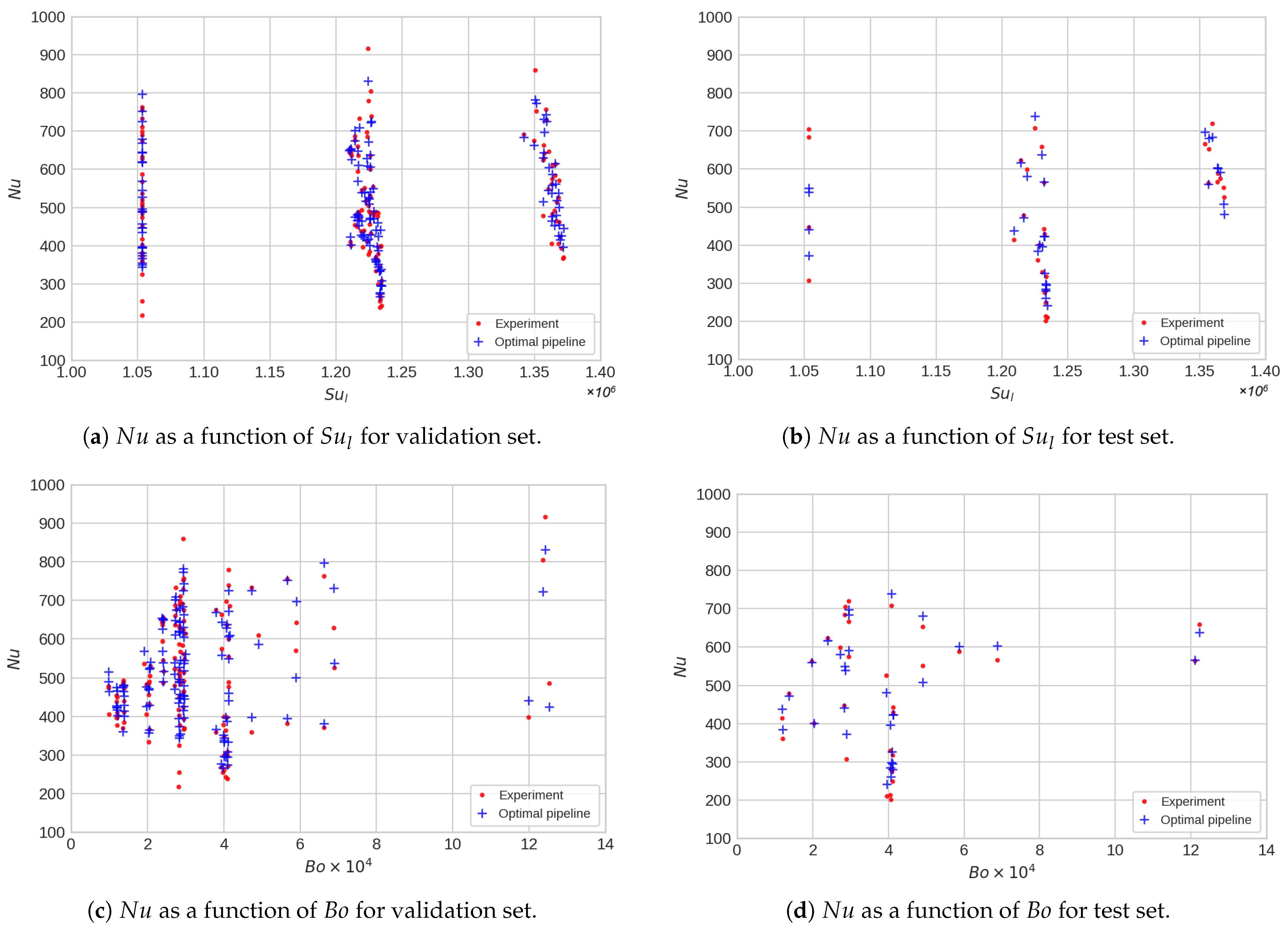
6.3. Machine Learning Pipeline Optimization

In the final step, the ML-based pipeline’s configuration, including the utilized algorithm and the corresponding tuning parameters along with the employed feature processing steps, is optimized. This procedure makes use of a genetic algorithm optimization method, in which the characteristics of the pipeline (including different sequences of feature processors and ML algorithms) are progressively improved, aiming at minimizing the considered fitness function (estimation MARD). The final solution with the lowest achieved MARD is then proposed as the optimal pipeline.
Table 8 exhibits the optimal pipeline proposed by the optimization procedure. It includes six steps: three estimators (ExtraTreesRegressor, ElasticNetCV, and RidgeCV) and three feature processors (MaxAbsScaler, RobustScaler, and PolynomialFeatures). Table 7 also reports the prediction accuracies obtained by this pipeline. It demonstrates that it manages to reduce the achieved MARD value for the validation set from 9.97% to 7.71%, and the MARD value obtained for the test set from 12.4% to 8.84%.
Figure 7 illustrates the estimations provided by the optimal pipeline (blue dots) and those offered by Rollmann and Spindler’s model (red dots) as a function of the experimental values for both validation and test sets. As this figure evidences, utilizing the achieved optimal pipeline leads to a notable improvement in the prediction accuracy compared to the most accurate physical model. The optimal pipeline’s prediction points fall more or less within a ± 15 % margin for both validation and test sets. Additionally, the best empirical model offers overall MARD values of 23.1% on the validation set and 19.7% on the test set. The comparison of these values with those of the optimal pipeline noted in Table 7 also shows the superior performance of the proposed optimal pipeline.
The authors of the present study did not find any other similar research that primarily focuses on employing machine learning-based models for heat transfer predictions for microfin tubes. However, the study conducted by Zhou et al. [30] shares a similar objective as the present research for serrated fins. The artificial neural network model proposed by that study managed to achieve an MARD of 11.41% employing the selected features.
Figure 8 and Figure 9 compare the experimental N u with the predictions of the optimal pipeline as a function of the most promising features. These figures show that the optimal pipeline achieves a relatively universal performance over a wide range of values of the selected features. Each of these features represents different physical phenomena, and thus, the optimal pipeline manages to take into account several aspects of the evaporation of the refrigerants in the microfin tubes.

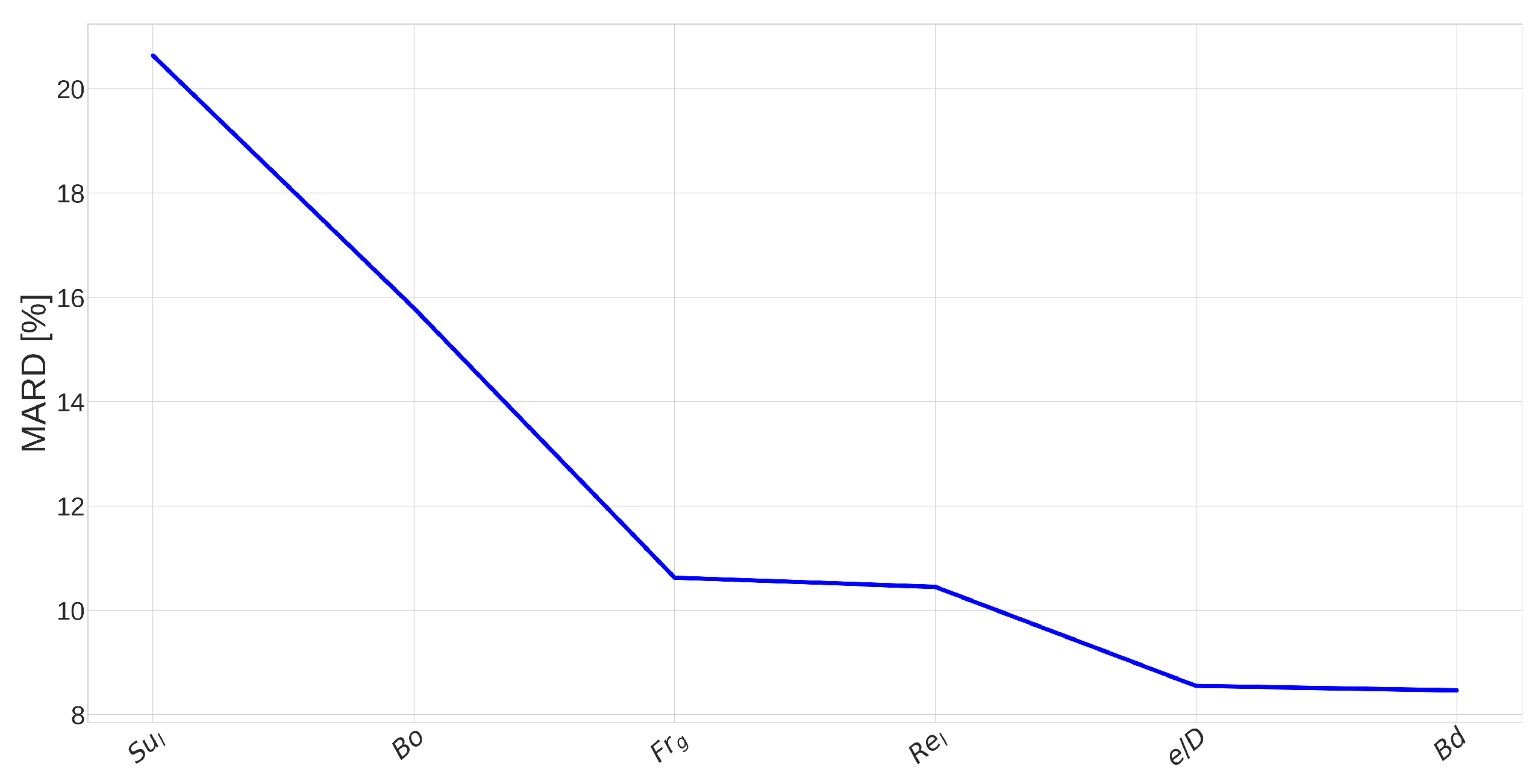
6.4. Forward Feature Combination

In the final step, in order to demonstrate the contribution of each dimensionless feature to the achieved accuracy, the forward feature combination procedure is implemented. The resulting diagram, which demonstrates the accuracy that is obtained after adding each feature, is depicted in Figure 10. As can be observed, by utilizing only the first three features ( S u l , B o , and F r g ), an MARD value close to 10.62% can be achieved. Adding the rest of the features only reduces the error by nearly 2% (reaching an MARD of 8.84%). Following the latter observation, the final user has the option of providing the proposed optimal pipeline with only the first three features (which notably simplifies the model and enhances the corresponding ease of use) while achieving an acceptable accuracy. It is noteworthy that although the geometrical parameter ( e d ) seems to have a negligible effect on the achieved accuracy, the hydraulic diameter (utilized in the calculation of the Suratman number, S u l ) already takes into account the corresponding impact.

7. Conclusions

The present study proposed a novel optimized machine learning pipeline to estimate the heat transfer in evaporating R134a flow streaming in horizontal microfin tubes. A set of experimental activities were carried out to build up the required heat transfer dataset. Then, the dataset was divided into training (and validation) and test subsets. The first subset was used to train the ML models, validate the corresponding performance, and determine the optimal pipeline. The test set was instead used to assess the estimation performance of the obtained optimal ML model for a dataset for which it was not optimized. In the training process, the Nusselt number was the target of the predictions and a set of dimensionless parameters were utilized as features. Firstly, an in-house feature selection algorithm was applied to the training set and defined the most promising features. Next, the pipeline optimization tool took the selected features of the training set and built up the optimized machine learning pipeline, resulting in a boosted accuracy. Well-known and widely adopted empirical models were selected from the literature and implemented to be the basis of the comparison with the proposed model. Then, the proposed pipeline and also the empirical models were applied to the test set, and their prediction performances were compared. The findings are summarized as follows:
  • The feature selection algorithm managed to select 6 features ( S u l , B o , F r g , R e l , B d , e / D ) among the pool of 21 features. The physical interpretation of the selected features confirmed their higher order of relevance to the target of the predictions.
  • The optimized pipeline improved the prediction accuracy and obtained an MARD value of 7.71% on the validation set and an MARD value of 8.84% on the test set, while the most promising empirical model (Rollmann and Spindler’s model Equation (19)) achieved MARD values of 23.1% and 19.7%, respectively on the validation and the test sets. Moreover, the proposed optimal pipeline accompanied by the employed dataset will be made publicly available.
  • In future works, the employed dataset should be extended, incorporating data obtained from multiple experimental facilities, which will permit training the algorithms using the data belonging to a test rig while utilizing datasets obtained from other experimental facilities as the test set [30,60,61,62].
  • Finally, it should be noted the main contribution of this study, beyond proposing an algorithm resulting in an elevated performance (even if only over the considered dataset), is identifying the most promising set of dimensionless features, which facilitates the corresponding physical interpretation.

Author Contributions

Conceptualization, B.N. and L.P.M.C.; Methodology, S.M., K.A., B.N. and L.P.M.C.; Software, S.M. and F.D.J.; Validation, S.M., K.A. and A.L.; Formal analysis, S.M. and K.A.; Resources, A.L. and I.M.C.; Data curation, S.M., K.A., F.D.J. and A.L.; Writing—original draft, S.M., K.A. and F.D.J.; Writing—review & editing, B.N. and I.M.C.; Supervision, B.N. and L.P.M.C. All authors have read and agreed to the published version of the manuscript.

Funding

This research received no external funding.

Data Availability Statement

The experimental dataset, the feature selection algorithm, and the optimal pipeline are available in the following online repository: https://github.com/DataOptimaLab/ML4EvapHeatTransfer (accessed on 12 June 2024).

Conflicts of Interest

The authors declare no conflicts of interest.

References

  1. Thome, J.R.; Favrat, D.; Kattan, N. Evaporation in Microfin Tubes: A Generalized Prediction Model; Technical Report; Taylor & Francis: Oxfordshire, UK, 1999. [Google Scholar]
  2. Cavallini, A.; Del Col, D.; Doretti, L.; Longo, G.A.; Rossetto, L. Refrigerant vaporization inside enhanced tubes: A heat transfer model. Heat Technol. 1999, 17, 29–36. [Google Scholar]
  3. Yun, R.; Kim, Y.; Seo, K.; Young Kim, H. A generalized correlation for evaporation heat transfer of refrigerants in micro-fin tubes. Int. J. Heat Mass Transf. 2002, 45, 2003–2010. [Google Scholar] [CrossRef]
  4. Chamra, L.M.; Mago, P.J. Modelling of evaporation heat transfer of pure refrigerants and refrigerant mixtures in microfin tubes. Proc. Inst. Mech.Eng. Part C J. Mech. Eng. Sci. 2007, 221, 443–454. [Google Scholar] [CrossRef]
  5. Rollmann, P.; Spindler, K. New models for heat transfer and pressure drop during flow boiling of R407C and R410A in a horizontal microfin tube. Int. J. Therm. Sci. 2016, 103, 57–66. [Google Scholar] [CrossRef]
  6. Han, X.H.; Fang, Y.B.; Wu, M.; Qiao, X.G.; Chen, G.M. Study on flow boiling heat transfer characteristics of R161/oil mixture inside horizontal micro-fin tube. Int. J. Heat Mass Transf. 2017, 104, 276–287. [Google Scholar] [CrossRef]
  7. Mehendale, S. A new heat transfer coefficient correlation for pure refrigerants and near-azeotropic refrigerant mixtures flow boiling within horizontal microfin tubes. Int. J. Refrig. 2018, 86, 292–311. [Google Scholar] [CrossRef]
  8. Dai, B.; Wu, T.; Liu, S.; Qi, H.; Zhang, P.; Wang, D.; Wang, X. Flow boiling heat transfer characteristics of zeotropic mixture CO2/R152a with large temperature glide in a 2 mm horizontal tube. Int. J. Heat Mass Transf. 2024, 218, 124779. [Google Scholar] [CrossRef]
  9. Mikielewicz, D.; Mikielewicz, J.; Tesmar, J. Improved semi-empirical method for determination of heat transfer coefficient in flow boiling in conventional and small diameter tubes. Int. J. Heat Mass Transf. 2007, 50, 3949–3956. [Google Scholar] [CrossRef]
  10. Pysz, M.; Mikielewicz, D. Flow boiling of R1233zd (E) in a 3 mm vertical tube at moderate and high reduced pressures. Exp. Therm. Fluid Sci. 2023, 147, 110964. [Google Scholar] [CrossRef]
  11. Hastie, T.; Tibshirani, R.; Friedman, J. Introduction. In The Elements of Statistical Learning: Data Mining, Inference, and Prediction; Springer: New York, NY, USA, 2009; pp. 1–8. [Google Scholar] [CrossRef]
  12. Abbassi, A.; Bahar, L. Application of neural network for the modeling and control of evaporative condenser cooling load. Appl. Therm. Eng. 2005, 25, 3176–3186. [Google Scholar] [CrossRef]
  13. Lecoeuche, S.; Lalot, S.; Desmet, B. Modelling a non-stationary single tube heat exchanger using multiple coupled local neural networks. Int. Commun. Heat Mass Transf. 2005, 32, 913–922. [Google Scholar] [CrossRef]
  14. Díaz, G.; Sen, M.; Yang, K.; McClain, R.L. Dynamic prediction and control of heat exchangers using artificial neural networks. Int. J. Heat Mass Transf. 2001, 44, 1671–1679. [Google Scholar] [CrossRef]
  15. Díaz, G.; Sen, M.; Yang, K.T.; McClain, R.L. Simulation of Heat Exchanger Performance by Artificial Neural Networks. HVAC&R Res. 1999, 5, 195–208. [Google Scholar] [CrossRef]
  16. Bar, N.; Bandyopadhyay, T.K.; Biswas, M.N.; Das, S.K. Prediction of pressure drop using artificial neural network for non-Newtonian liquid flow through piping components. J. Pet. Sci. Eng. 2010, 71, 187–194. [Google Scholar] [CrossRef]
  17. Pacheco-Vega, A.; Sen, M.; McClain, R.L. Analysis of fin-tube evaporator performance with limited experimental data using artificial neural networks. In Proceedings of the ASME 2000 International Mechanical Engineering Congress and Exposition, Orlando, FL, USA, 5–10 November 2000; Volume 366, pp. 95–101. [Google Scholar]
  18. Najafi, B.; Ardam, K.; Hanušovský, A.; Rinaldi, F.; Colombo, L.P.M. Machine learning based models for pressure drop estimation of two-phase adiabatic air-water flow in micro-finned tubes: Determination of the most promising dimensionless feature set. Chem. Eng. Res. Des. 2021, 167, 252–267. [Google Scholar] [CrossRef]
  19. Ardam, K.; Najafi, B.; Lucchini, A.; Rinaldi, F.; Colombo, L.P.M. Machine learning based pressure drop estimation of evaporating R134a flow in micro-fin tubes: Investigation of the optimal dimensionless feature set. Int. J. Refrig. 2021, 131, 20–32. [Google Scholar] [CrossRef]
  20. Rashidi, M.; Nazari, M.A.; Harley, C.; Momoniat, E.; Mahariq, I.; Ali, N. Applications of machine learning methods for boiling modeling and prediction: A comprehensive review. Chem. Thermodyn. Therm. Anal. 2022, 8, 100081. [Google Scholar] [CrossRef]
  21. Bouali, A.; Hanini, S.; Mohammedi, B.; Boumahdi, M. Using artificial neural network for predicting heat transfer coefficient during flow boiling in an inclined channel. Therm. Sci. 2021, 25, 3911–3921. [Google Scholar] [CrossRef]
  22. Thibault, J.; Grandjean, B.P.A. A neural network methodology for heat transfer data analysis. Int. J. Heat Mass Transf. 1991, 34, 2063–2070. [Google Scholar] [CrossRef]
  23. Jambunathan, K.; Hartle, S.L.; Ashforth-Frost, S.; Fontama, V.N. Evaluating convective heat transfer coefficients using neural networks. Int. J. Heat Mass Transf. 1996, 39, 2329–2332. [Google Scholar] [CrossRef]
  24. Chen, J.; Wang, K.; Liang, M. Predictions of heat transfer coefficients of supercritical carbon dioxide using the overlapped type of local neural network. Int. J. Heat Mass Transf. 2005, 48, 2483–2492. [Google Scholar] [CrossRef]
  25. Pacheco-Vega, A.; Sen, M.; Yang, K.T.; McClain, R.L. Neural network analysis of fin-tube refrigerating heat exchanger with limited experimental data. Int. J. Heat Mass Transf. 2001, 44, 763–770. [Google Scholar] [CrossRef]
  26. Scalabrin, G.; Condosta, M.; Marchi, P. Modeling flow boiling heat transfer of pure fluids through artificial neural networks. Int. J. Therm. Sci. 2006, 45, 643–663. [Google Scholar] [CrossRef]
  27. Scalabrin, G.; Condosta, M.; Marchi, P. Mixtures flow boiling: Modeling heat transfer through artificial neural networks. Int. J. Therm. Sci. 2006, 45, 664–680. [Google Scholar] [CrossRef]
  28. Zhao, L.; Zhang, C. Fin-and-tube condenser performance evaluation using neural networks. Int. J. Refrig. 2010, 33, 625–634. [Google Scholar] [CrossRef]
  29. Xie, G.N.; Wang, Q.W.; Zeng, M.; Luo, L.Q. Heat transfer analysis for shell-and-tube heat exchangers with experimental data by artificial neural networks approach. Appl. Therm. Eng. 2007, 27, 1096–1104. [Google Scholar] [CrossRef]
  30. Zhou, L.; Garg, D.; Qiu, Y.; Kim, S.; Mudawar, I.; Kharangate, C.R. Machine learning algorithms to predict flow condensation heat transfer coefficient in mini/micro-channel utilizing universal data. Int. J. Heat Mass Transf. 2020, 162, 120351. [Google Scholar] [CrossRef]
  31. Hughes, M.T.; Fronk, B.M.; Garimella, S. Universal condensation heat transfer and pressure drop model and the role of machine learning techniques to improve predictive capabilities. Int. J. Heat Mass Transf. 2021, 179, 121712. [Google Scholar] [CrossRef]
  32. Zhu, G.; Wen, T.; Zhang, D. Machine learning based approach for the prediction of flow boiling/condensation heat transfer performance in mini channels with serrated fins. Int. J. Heat Mass Transf. 2021, 166, 120783. [Google Scholar] [CrossRef]
  33. Moradkhani, M.; Hosseini, S.; Karami, M. Forecasting of saturated boiling heat transfer inside smooth helically coiled tubes using conventional and machine learning techniques. Int. J. Refrig. 2022, 143, 78–93. [Google Scholar] [CrossRef]
  34. Bard, A.; Qiu, Y.; Kharangate, C.R.; French, R. Consolidated modeling and prediction of heat transfer coefficients for saturated flow boiling in mini/micro-channels using machine learning methods. Appl. Therm. Eng. 2022, 210, 118305. [Google Scholar] [CrossRef]
  35. Colombo, L.P.M.; Lucchini, A.; Muzzio, A. Flow patterns, heat transfer and pressure drop for evaporation and condensation of R134A in microfin tubes. Int. J. Refrig. 2012, 35, 2150–2165. [Google Scholar] [CrossRef]
  36. Colombo, L.P.M.; Lucchini, A.; Phan, T.N.; Molinaroli, L.; Niro, A. Design and assessment of an experimental facility for the characterization of flow boiling of azeotropic refrigerants in horizontal tubes. J. Phys. Conf. Ser. 2019, 1224. [Google Scholar]
  37. Rinaldi, F.; Najafi, B. Temperature measurement in WTE boilers using suction pyrometers. Sensors 2013, 13, 15633–15655. [Google Scholar] [CrossRef] [PubMed]
  38. Vij, A.K.; Dunn, W. Modeling of Two-Phase Flows in Horizontal Tubes; Technical Report; Air Conditioning and Refrigeration Center, College of Engineering: Urbana, IL, USA, 1996. [Google Scholar]
  39. Lockhart, R.; Martinelli, R. Proposed correlation of data for isothermal two-phase, two-component flow in pipes. Chem. Eng. Prog. 1949, 45, 39–48. [Google Scholar]
  40. Breber, G.; Palen, J.W.; Taborek, J. Prediction of horizontal tubeside condensation of pure components using flow regime criteria. J. Heat Transf. 1980, 102, 471–476. [Google Scholar] [CrossRef]
  41. Papadopoulos, D.N.; Javan, F.D.; Najafi, B.; Mamaghani, A.H.; Rinaldi, F. Handling complete short-term data logging failure in smart buildings: Machine learning based forecasting pipelines with sliding-window training scheme. Energy Build. 2023, 301, 113694. [Google Scholar] [CrossRef]
  42. Najafi, B.; Bonomi, P.; Casalegno, A.; Rinaldi, F.; Baricci, A. Rapid fault diagnosis of PEM fuel cells through optimal electrochemical impedance spectroscopy tests. Energies 2020, 13, 3643. [Google Scholar] [CrossRef]
  43. Pearson, K. VII. Note on regression and inheritance in the case of two parents. Proc. R. Soc. Lond. 1895, 58, 240–242. [Google Scholar]
  44. Olson, R.S.; Bartley, N.; Urbanowicz, R.J.; Moore, J.H. Evaluation of a tree-based pipeline optimization tool for automating data science. In Proceedings of the Genetic and Evolutionary Computation Conference 2016, ACM, Denver, CO, USA, 20–24 July 2016; pp. 485–492. [Google Scholar]
  45. Le, T.T.; Fu, W.; Moore, J.H. Scaling tree-based automated machine learning to biomedical big data with a feature set selector. Bioinformatics 2020, 36, 250–256. [Google Scholar] [CrossRef]
  46. Najafi, B.; Najafi, H.; Idalik, M. Computational fluid dynamics investigation and multi-objective optimization of an engine air-cooling system using genetic algorithm. Proc. Inst. Mech. Eng. Part C J. Mech. Eng. Sci. 2011, 225, 1389–1398. [Google Scholar] [CrossRef]
  47. Mamaghani, A.H.; Najafi, B.; Casalegno, A.; Rinaldi, F. Optimization of an HT-PEM fuel cell based residential micro combined heat and power system: A multi-objective approach. J. Clean. Prod. 2018, 180, 126–138. [Google Scholar] [CrossRef]
  48. Selleri, T.; Najafi, B.; Rinaldi, F.; Colombo, G. Mathematical modeling and multi-objective optimization of a mini-channel heat exchanger via genetic algorithm. J. Therm. Sci. Eng. Appl. 2013, 5. [Google Scholar] [CrossRef]
  49. Lukman, A.F.; Ayinde, K.; Ajiboye, A.S. Monte Carlo study of some classification-based ridge parameter estimators. J. Mod. Appl. Stat. Methods 2017, 16, 24. [Google Scholar] [CrossRef]
  50. Zou, H.; Hastie, T. Regularization and variable selection via the elastic net. J. R. Stat. Soc. Ser. B Stat. Methodol. 2005, 67, 301–320. [Google Scholar] [CrossRef]
  51. Farajzadeh-Zanjani, M.; Razavi-Far, R.; Saif, M. Efficient sampling techniques for ensemble learning and diagnosing bearing defects under class imbalanced condition. In Proceedings of the 2016 IEEE Symposium Series on Computational Intelligence (SSCI), Athens, Greece, 6–9 December 2016; pp. 1–7. [Google Scholar] [CrossRef]
  52. Dadras Javan, F.; Campodonico Avendano, I.A.; Najafi, B.; Moazami, A.; Rinaldi, F. Machine-Learning-Based Prediction of HVAC-Driven Load Flexibility in Warehouses. Energies 2023, 16, 5407. [Google Scholar] [CrossRef]
  53. Manivannan, M.; Najafi, B.; Rinaldi, F. Machine learning-based short-term prediction of air-conditioning load through smart meter analytics. Energies 2017, 10, 1905. [Google Scholar] [CrossRef]
  54. Pedregosa, F.; Varoquaux, G.; Gramfort, A.; Michel, V.; Thirion, B.; Grisel, O.; Blondel, M.; Prettenhofer, P.; Weiss, R.; Dubourg, V.; et al. Scikit-learn: Machine learning in Python. J. Mach. Learn. Res. 2011, 12, 2825–2830. [Google Scholar]
  55. Breirnan, L. Arcing classifiers. Ann. Stat. 1998, 26, 801–849. [Google Scholar]
  56. Razavi-Far, R.; Farajzadeh-Zanjani, M.; Chakrabarti, S.; Saif, M. Data-driven prognostic techniques for estimation of the remaining useful life of lithium-ion batteries. In Proceedings of the 2016 IEEE International Conference on Prognostics and Health Management (ICPHM), Ottawa, ON, Canada, 20–22 June 2016; pp. 1–8. [Google Scholar] [CrossRef]
  57. Najafi, B.; Di Narzo, L.; Rinaldi, F.; Arghandeh, R. Machine learning based disaggregation of airconditioning loads using smart meter data. IET Gener. Transm. Distrib. 2020, 14, 4755–4762. [Google Scholar] [CrossRef]
  58. Geurts, P.; Ernst, D.; Wehenkel, L. Extremely randomized trees. Mach. Learn. 2006, 63, 3–42. [Google Scholar] [CrossRef]
  59. Bisong, E.; Bisong, E. Introduction to Scikit-learn. In Building Machine Learning and Deep Learning Models on Google Cloud Platform: A Comprehensive Guide for Beginners; Springer: Berlin/Heidelberg, Germany, 2019; pp. 215–229. [Google Scholar]
  60. Nie, F.; Wang, H.; Zhao, Y.; Song, Q.; Yan, S.; Gong, M. A universal correlation for flow condensation heat transfer in horizontal tubes based on machine learning. Int. J. Therm. Sci. 2023, 184, 107994. [Google Scholar] [CrossRef]
  61. Qiu, Y.; Garg, D.; Zhou, L.; Kharangate, C.R.; Kim, S.M.; Mudawar, I. An artificial neural network model to predict mini/micro-channels saturated flow boiling heat transfer coefficient based on universal consolidated data. Int. J. Heat Mass Transf. 2020, 149, 119211. [Google Scholar] [CrossRef]
  62. Moradkhani, M.; Hosseini, S.; Song, M. Robust and general predictive models for condensation heat transfer inside conventional and mini/micro channel heat exchangers. Appl. Therm. Eng. 2022, 201, 117737. [Google Scholar] [CrossRef]
Figure 1. Schematic representation of a microfin tube.
Energies 17 04074 g001
Figure 5. The flowchart illustrating the adopted methodology of the current work.
Energies 17 04074 g005
Figure 6. Evaporation N u estimation based on the model proposed by Rollmann and Spindler [5] compared to the experimental N u .
Energies 17 04074 g006
Figure 7. Comparison of N u number, predicted by optimal pipeline and calculated by Rollmann and Spindler empirical model [5], with experimental N u .
Energies 17 04074 g007
Figure 8. Comparison of experimental Nusselt number with predictions of the optimal pipeline as a function of S u l and B o .
Energies 17 04074 g008
Figure 9. Comparison of experimental Nusselt number with predictions of optimal pipeline as a function of F r g and R e l .
Energies 17 04074 g009
Figure 10. Forward feature combination for evaporation ML pipeline.
Energies 17 04074 g010
Table 1. Specification of tubes.
ParametersTubesUnits
Microfin 1 Microfin 2 Microfin 3
Name of the tubeJ-60VA 1HVA 1[-]
External diameter9.529.529.52mm
Internal diameter8.968.928.62mm
Thickness0.280.30.45mm
Cross-section area62.1361.7257.33mm2
Wet perimeter42.3839.947.72mm
Rx1.681.61.88[-]
Fin typeAJ-60AVABVAAHVABHVA
Fin height0.20.230.160.20.17mm
Apex angle4040404040[○]
No. of fins6027274141[-]
Helix angle1818181818[○]
1 Microfin tubes VA and HVA have an alternation of two different sizes of fin which are placed sequentially after one another.
Table 2. The specifications of the utilized measurement devices.
Measurement ParametersDeviceRangeUnitUncertainty
Demineralized water mass flow rateCoriolis flow meter0;400 kg s 0.15% of the reading
Coriolis flow meter0;6500 kg s 0.3% of the reading
Refrigerant mass flow rateCoriolis flow meter0;400 kg s 0.15% of the reading
Water temperatureThermocouples type K−180;1350[°C]0.1 K
Refrigerant temperatureThermocouples type K−180;1350[°C]0.1 K
Refrigerant inlet pressureRelative pressure transducer0;16 [ bar g ] 0.2% of full scale
Pressure dropDifferential pressure transducer−15;15[psi]0.1% of full scale
Test section tube length-2000mm6 mm
Voltage of electric heater---1% of the reading
Current of electric heater---1% of the reading
Table 3. The thermal and fluid conditions of the experiments.
Parameters ConditionTubesUnits
J60 VA HVA
Number of data pointsEvaporation864033[-]
Mass fluxes range66.3–380.390–315.696.7–339.6 [ kg ( m 2 s ) ]
Mass quality range0.15–0.950.25–0.750.45–0.8[-]
Heat transfer coefficient range2023–92043701–86952271–7957 W ( m 2 K )
Table 6. Accuracy of the empirical models for the two-phase evaporating flow.
Empirical ModelMRD [%]MARD [%]
Mehendale (2017) [7]54.9469.7
Han et al. (2017) [6]−56.3856.63
Rollmann and Spindler (2016) [5]18.5122.42
Chamra and Magro (2006) [4]−20.9828.24
Yun et al. (2002) [3]−83.0683.06
Cavallini et al. (1999) [2]22.5234.39
Thome et al. (1997) [1]80.2980.29
Table 7. The prediction accuracies of the pipelines trained with different feature sets.
PipelineInput FeaturesValidation Set (CV)Test Set
MRD [%] MARD [%] MRD [%] MARD [%]
All features—RF R e l , R e g , W e l , W e g 2.0510.424.6412.54
F r l , F r g , P r l , P r g , B o , P r e
B d , K a , C o , G a , S u f , S u g
J g , X t t , n, e / D , R x
Selected features—RF S u l , B o , F r g , R e l , B d , e / D 1.769.973.9412.4
Selected features—optimized pipeline S u l , B o , F r g , R e l , B d , e / D 1.547.713.328.84
Table 8. The optimal pipeline description (Scikit-learn: Machine Learning in Python, Pedregosa et al. [54]).
Optimal PipelineArgumentsDefinitionsValues
Step one:
ExtraTreesRegressor
bootstrapWhether the bootstraps are used when building the treesFalse
max_featuresThe number of considered features when building the trees0.35
min_samples_leafThe minimum number of samples at each leaf node3
min_samples_splitThe minimum number of samples to split an internal node15
n_estimatorThe number of the trees in the forest100
Step two:
MaxAbsScaler
--2
Step three:
ElasticNetCV
l1_ratioThe value shows the inclination toward L1 or L2 penalty0.1
tolThe tolerance of the optimization0.0001
Step four:
RobustScaler
---
Step five:
PolynomialFeatures
degreeThe degree of the polynomial2
include_biasIf True, adding an intercept term to the polynomialFalse
interaction_onlyIf True, only interaction features are producedFalse
Step six:
RidgeCV
---
Disclaimer/Publisher’s Note: The statements, opinions and data contained in all publications are solely those of the individual author(s) and contributor(s) and not of MDPI and/or the editor(s). MDPI and/or the editor(s) disclaim responsibility for any injury to people or property resulting from any ideas, methods, instructions or products referred to in the content.

