Abstract
Using renewable energies is one of the alternatives to mitigate climate change. Among them, photovoltaic energy has shown a relevant growth of participation in the electric sector. In the backdrop of such growth, in countries such as Brazil, photovoltaic energy has surpassed the generation of electricity by petroleum derivatives since 2019. The significant growth in photovoltaic generation around the world can be attributed to several key factors, including abundant sunlight, supportive government policies, falling solar panel costs, environmental concerns, energy diversification goals, investor interest, job creation, and local manufacturing. However, photovoltaic system performance is heavily tied to weather variability. Different models are used to account for this meteorological dependence; however, there is a gap regarding the differences in the outputs of these models. The study presented here investigates the variability and sensitivity of the models used to estimate photovoltaic production (). Six models were compared by percentage difference analysis. Statistical analyses from the perspective of variability revealed that the difference between the estimated by these models reaches a 12.89% absolute power difference. Considering that temperature and solar irradiance are the meteorological variables that most influence , the sensitivity analysis focused on these. Regarding sensitivity, in the context of temperature changes, the average relative difference in between models can reach up to 5.32% for a 10 °C change, while in the context of changes in solar irradiance, the average relative difference can reach up to 19.05% for a change of 41.67 W/m2. The consideration of the variability and sensitivity of the main sets of equations used to estimate the potential of photovoltaic energy production can help refine methodologies and assumptions in future research in this area. There are variations and sensitivities, as observed, of such magnitude that, depending on the set of equations adopted in the study, they can alter the conclusion about photovoltaic energy production in a given region. Accurate estimations are pivotal not only for feasibility analyses but also for gauging economic and socio-environmental impacts. These divergences can, in turn, reformulate feasibility analyses and compromise the reliability of photovoltaic energy systems, thus leading to different economic and socio-environmental consequences.
1. Introduction
Renewable energies are considered a fundamental tool to advance towards the United Nations Sustainable Development Goal number 7, which implies universal access to affordable, reliable, and modern energy [1]. Renewable energies can also help reduce global greenhouse gas emissions and thus mitigate climate change. Among renewable energy projects, decentralized projects based on solar photovoltaic (PV) systems have the potential to contribute to climate change adaptation, climate resilience, energy security, and social justice [2]. However, the sensitivity of renewable energies to future climate variability is a source of uncertainty that can complicate energy planning and jeopardize investments in the energy sector.
Changes in the frequency of days with high air temperatures or cloudy days can substantially alter the yields of photovoltaic systems. Photovoltaic production () describes the performance of photovoltaic cells in relation to their nominal power generation capacity according to the actual conditions of the environment [3]. depends on the solar resource available at the site, air temperature, wind speed, cloud cover, aerosols, spectral distribution of incident irradiance, angle of incidence of irradiance, and operating efficiency of system components [4]. Many works address this topic. Zuluaga et al. (2022) [5] projected the energy production potential of photovoltaic systems under different climate change scenarios for Brazil. For the short-term future (2021–2050), they estimated increases for the North Region. However, in the long term (2071–2100), significant decreases are predicted for the entire country (except for the extreme north). Zhang et al. (2022) [6] quantified the impact of climate change on photovoltaic potential for China, considering the average and extreme conditions of solar inputs, indicating a decrease in the face of warmer weather. Niu et al. (2023) [7] analyzed the spatial and temporal variations of photovoltaic power potential for China. They indicated a decrease in the potential for photovoltaic energy, considering a scenario of high resource use and dependence on fossil fuels. However, the potential for photovoltaic energy would increase towards a more sustainable scenario. They also estimated the contribution of surface radiation, aerosols, and cloud cover. Ha et al. (2023) [8] globally studied the consequences of climate projections in different greenhouse gas emission scenarios and indicated high vulnerability in the supply of solar energy due to rising temperatures.
Different models of PV modules have been developed, from simple models with few input parameters to more complex models with extensive PV module modeling procedures [9]. It is common to classify them into two categories: (1) power models, and (2) models based on the equivalent electrical circuit of the photovoltaic cell [10]. In the present study, we focused on the models of the first group due to their simplicity and wide adoption in the economic feasibility studies of PV plants around the world.
In the literature, two linear negative gradient relationships are established for the efficiency of a PV cell as a function of cell temperature (Equation (1)) and combined temperature and solar irradiance (Equation (2)).
where is the reference efficiency, is the solar irradiance, and are respectively the coefficients of temperature and irradiance defined by the cell material and structure, and and are, respectively, cell temperature and the reference temperature of 25 °C [11,12,13,14].
In Equation (1), assumes the value of 0.005/°C for monocrystalline silicon cells [14], and in Equation (2), /°C and must be used [15]. In Equation (2), the reduction in PV cell efficiency due to low luminosity levels is considered by means of [7].
While total irradiance can be measured directly, cell temperature cannot, and some relationships have been developed to determine it. In the sequence of studies of several authors [16,17,18], a general empirical expression for cell temperature was defined according to Equation (3).
where is the ambient temperature in °C.
The coefficients depend on the details of the module and assembly that affect the heat transfer of the cell. The coefficients normally used in this equation were obtained from the study conducted by Lasnier and Ang (1990) [18] for a monocrystalline silicon cell, namely: °C, and °C·m2/W.
Jerez et al. (2015) [3] used Equation (1), but did not use Equation (3). In fact, the authors proposed the use of a new equation including the influence of wind speed, according to Chenni et al. (2007) [15] (Equation (4)).
where is the wind speed at the earth’s surface in m/s.
According to Chenni et al. (2007) [19], the coefficients for a monocrystalline silicon cell are °C, , °C·m2/W and °C·s/m. Therefore, if the environmental conditions (, and ) correspond to the standard test conditions (STCs), PV energy production reaches the nominal value. If they are such that is greater than 25 °C and/or is lower than 1000 W/m2, the PV power output will be less than the nominal power of the module.
Pérez et al. (2019) changed the values of the coefficients to °C, , °C m2/W and °C·s/m, as established by Mavromatakis et al. (2014) [20]. Pérez et al. (2019) [21] emphasized that this new linear model is not suitable for wind speeds greater than 10 m/s, as these conditions produce an unrealistic low temperature of the module.
Sawadogo et al. (2020) [22] used the same Equation (1) as Jerez et al. (2015) [3], but replaced Equation (4) with Equation (5).
where is the relative humidity in %.
According to TamizhMani et al. (2003) [23], the system-specific regression coefficients are °C, , °C·m2/W, °C·s/m, and °C/%.
Some other relationships to describe the dependence of the photovoltaic cell temperature on the meteorological variables have been used. Zou et al. (2019) [24] used Equation (6).
where is the nominal operating cell temperature, which is defined as the temperature that is reached when the cells are mounted in a location with a solar irradiance level of 800 W/m2, wind speed of 1 m/s, and ambient temperature of 20 °C.
Smith et al. (2017) [25] used Equation (7) to define cell temperature.
which assumes that the PV module is mounted in an open field and that the free-flowing wind speed does not strongly influence convection heat transfer, with = 0.2933 K/W·m2 [25].
Unlike all previous studies, Gunderson et al. (2015) [26] opted for a simplistic model (Equation (8)).
that is, it assumes that the PV cell efficiency is constant and that the potential for photovoltaic energy generation depends only on solar irradiance, not taking into account the other meteorological variables.
A synthesis of the equations presented is shown in Table 1.
It is important to emphasize that none of the above equations present, as input, variables that explicitly represent the influence of dust, wind direction, irradiance incidence angle, and PV module material. Therefore, they are considered implicitly in terms of existing equations or in the treatment of data prior to the use of the aforementioned equations, which is the approach Bazyomo et al. (2016) [27] used when calculating solar irradiance on a tilted plane using the free R solar package, solaR [28].

Table 1.
Models used to consider the impact of meteorological variables on PV production.
Table 1.
Models used to consider the impact of meteorological variables on PV production.
| # | Papers | Equations | Primary Reference 1 |
|---|---|---|---|
| 1 | [24,29] | : [30,31] : [32] | |
| 2 | [3,15,27,33,34,35] | : [30,31] : [18] | |
| 3 | [25] | : [30,31] : [36] | |
| 4 | [22] | : [37] : [23] | |
| 5 | [2,3,21,38] | : [37] : [23] | |
| 6 | [26] | : [39] : - 2 |
1 Primary reference is the study that developed and/or first used the equation. It is not necessarily the study that was cited by the authors of the studies, in column 2, to justify its use to estimate . Example: ‘A’ cites ‘B’, which cites ‘C’, which cites ‘D’; the primary reference for the study of ‘A’ is ‘D’, not ‘B’. There may be more than one primary reference when the precursor study is not evident. 2 The model M6 assumes that the PV cell efficiency is constant, not taking into account the meteorological variables. Thus, there is no equation to estimate .
Thus, it can be observed that there is no consensus in the literature on which set of equations should be used to estimate photovoltaic production , and there is no study comparing the main models used. Therefore, the objective of this study is to analyze the variability and sensitivity of the main sets of equations used to estimate . In other words, the aim of this study was not to assess which model is the most accurate, but rather to examine the differences in results when compared to each other. These distinctions were determined within the context of variability and sensitivity to changes in ambient temperature and solar irradiance. The paper is structured as follows: Section 2 provides clarification on the data and models compared, as well as the methodology used; Section 3 presents the results and discusses them based on statistical analyses; and Section 4 summarizes the conclusions and the implications arising from this study.
2. Methodology
2.1. Determination of the Models
The models were defined based on what was present in the literature (Table 1) and were found to be the most recurrent in determining the potential for photovoltaic energy production (Table 2). The M6 model used by Gunderson et al. (2015) [26] considers the PV cell efficiency to be constant, so there is no equation to define cell temperature, nor for the operational loss factor.
Table 2.
Models effectively compared.
2.2. Meteorological Data
The meteorological data are necessary to enable the comparative analysis of how different the outputs of the six models, M1 to M6, are in estimating when the same meteorological data are used. These meteorological data are required for the calculation of , which is followed by the analysis of variability (Section 2.4) and sensitivity (Section 2.5).
The data used were made available by the National Institute of Meteorology (INMET) from the historical database. Data from the conventional weather station (OMM code 82798) and the automatic weather station (OMM code 81918) belonging to the city of João Pessoa, capital of the state of Paraíba, northeastern Brazil, were used for the comparison. Monthly and daily data for the period between January 1961 and December 2021 were collected. The selected parameters were average air temperature, solar irradiation (converted to solar irradiance to enable the analyses performed here), average wind speed, and relative humidity.
The data in their integral form were organized by parameter in spreadsheets and then subjected to a quality control process to check for and eliminate errors derived from technical or data transmission problems. From then on, all the data were arranged monthly, using only complete years; that is, years in which data were obtained in all months from January to December.
2.3. Calculation of Photovoltaic Production ()
After defining the models to be compared using the climatic parameters detailed above and a chosen photovoltaic solar module, the photovoltaic production was calculated. The photovoltaic solar module selected was the Axitec AC 260P/156-60S model, commonly used in the region. Table 3 shows the technical characteristics of the solar module [40].
Table 3.
Characteristics of the photovoltaic solar module.
, as a function of meteorological variables, was calculated from Equation (9) [41].
where is the number of modules considered, is the area of a PV module, is the efficiency of the PV module, is the solar irradiance, and is the operational loss factor.
The calculations were performed considering 100 modules. The calculation of average uses daily data of and to establish the monthly average, and only then performs the calculations using the equations identified previously. Small errors will arise from the nonlinear term of and in Equation (2) because the variation of and throughout the day is an average. A numerical simulation under clear sky conditions suggests that errors range from 1% to 2% depending on latitude [15]. However, these errors are highly systematic and have little effect on the percentage variation in energy production when analyzed between different years [15].
2.4. Variability Analysis
The variability analysis sought to check how different the results from each of the six models compared can be. Such differences were quantified from the average relative difference between each pair of models, considering the lowest value to establish reference (Equation (10)). Thus, the final value was calculated as an average for the months of the year.
where is the result of the variable in the analysis of model j, is the result of the variable in the analysis of model i, and ARDV is the average relative difference in variability in %.
We opted for a relative analysis to remove the influence of the magnitude of the data involved in order to allow the results obtained here to be compared with those extracted from meteorological data of other regions.
2.5. Sensitivity Analysis
The sensitivity analysis sought to check how different the results from each of the six models compared can be when the variables air temperature and solar irradiance are altered. Such differences were quantified based on the average relative difference between the reference value and the value after artificial alteration (Equation (11)) of the meteorological variables (Table 4). Thus, the final value was calculated as an average for the months of the year.
where is the reference result of the variable in the analysis of model i, is the result after artificial alteration of the variable in the analysis of model i, and ARDS is the average relative difference in sensitivity in %.
Table 4.
Conditions for the sensitivity analysis of the compared models.
The variables air temperature and solar irradiance were forcibly altered, as described in Table 4, in order to identify the individual sensitivity of each model.
3. Results and Discussions
3.1. Variability of the Models
From Figure 1, Figure 2, Figure 3 and Figure 4, it is possible to observe that, despite using exactly the same climate database, the outputs of each of the five models analyzed have some distinctions that deserve to be pointed out. It is important to emphasize that the absence of equations for the parameters of cell temperature and operational loss factor—due to the methodology adopted by its creator—made it impossible to include the M6 model in Figure 1 and Figure 2.
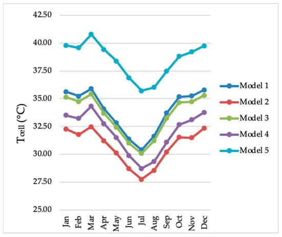
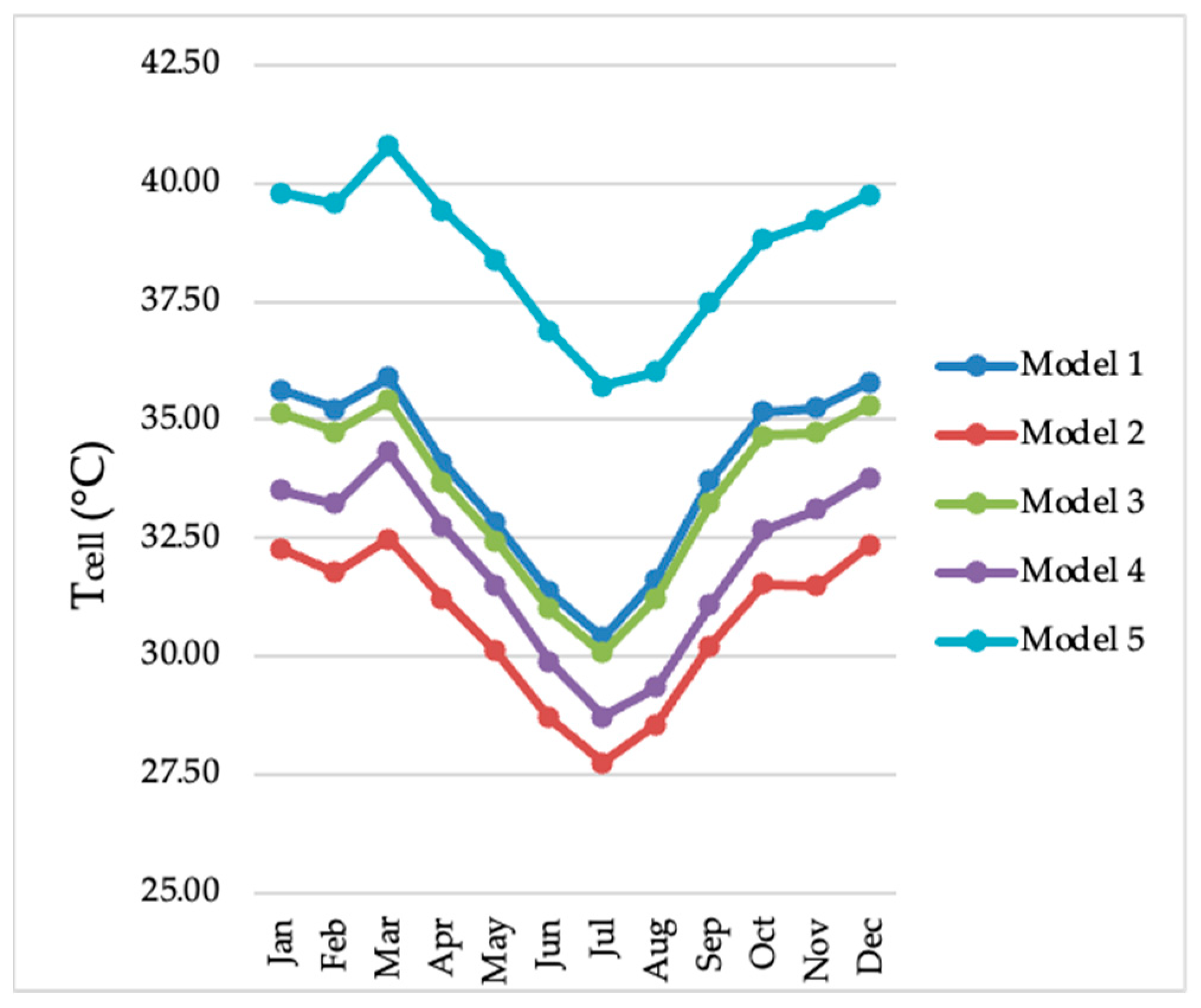
Figure 1.
Monthly average values of for the PV production calculation models in the city of João Pessoa, PB, Brazil, between the years 1961 and 2021 for 100 Axitec AC 260P/156-60S PV modules.
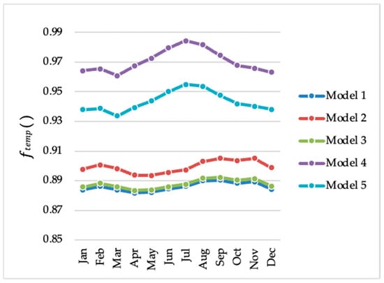
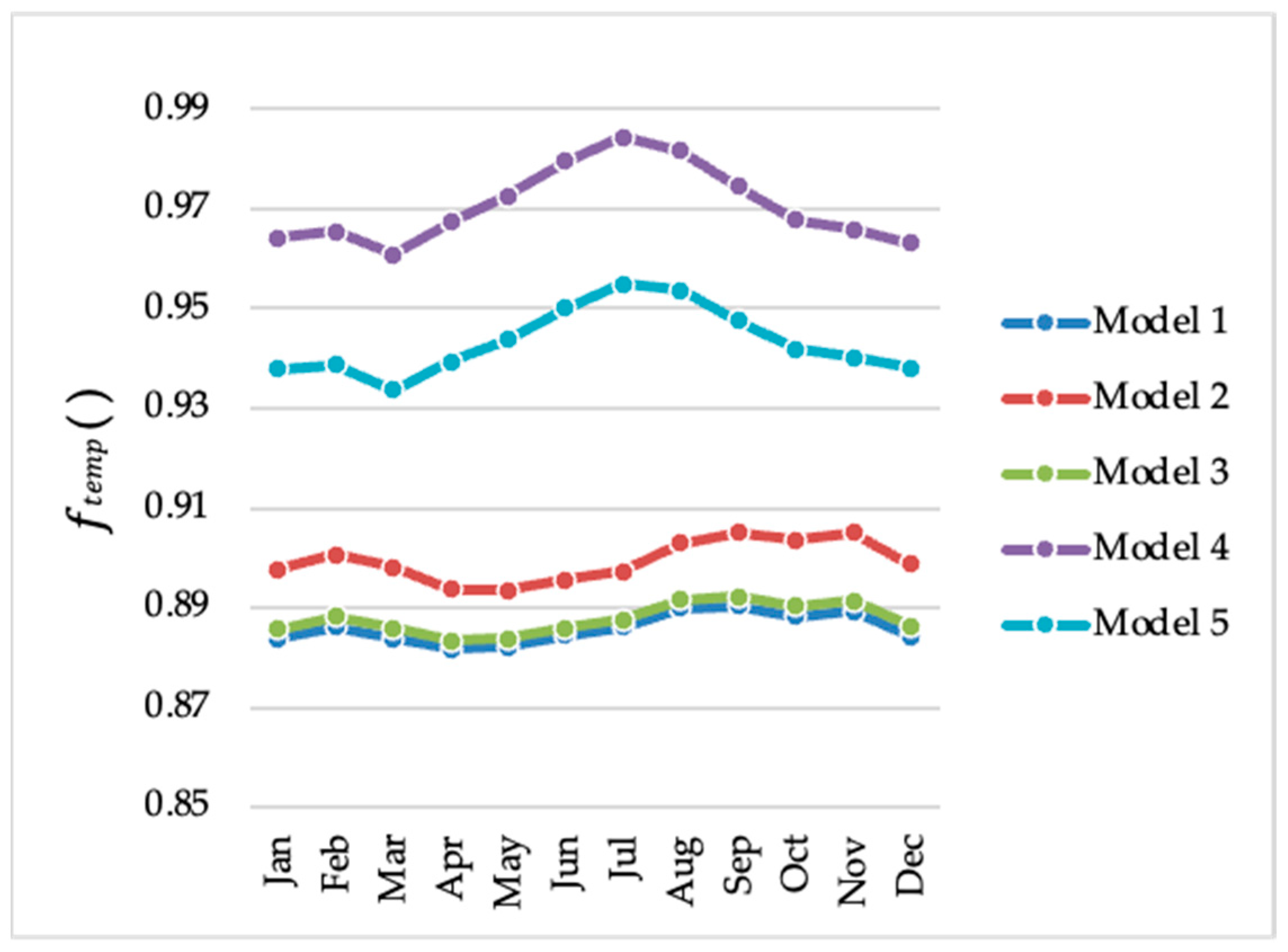
Figure 2.
values for PV production calculation models for the city of João Pessoa, PB, Brazil, between the years 1961 and 2021 for 100 Axitec AC 260P/156-60S PV modules.
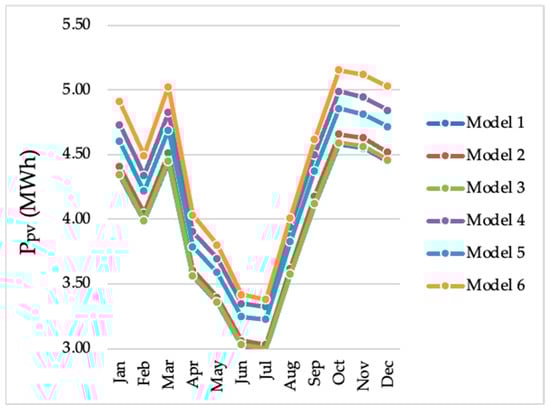
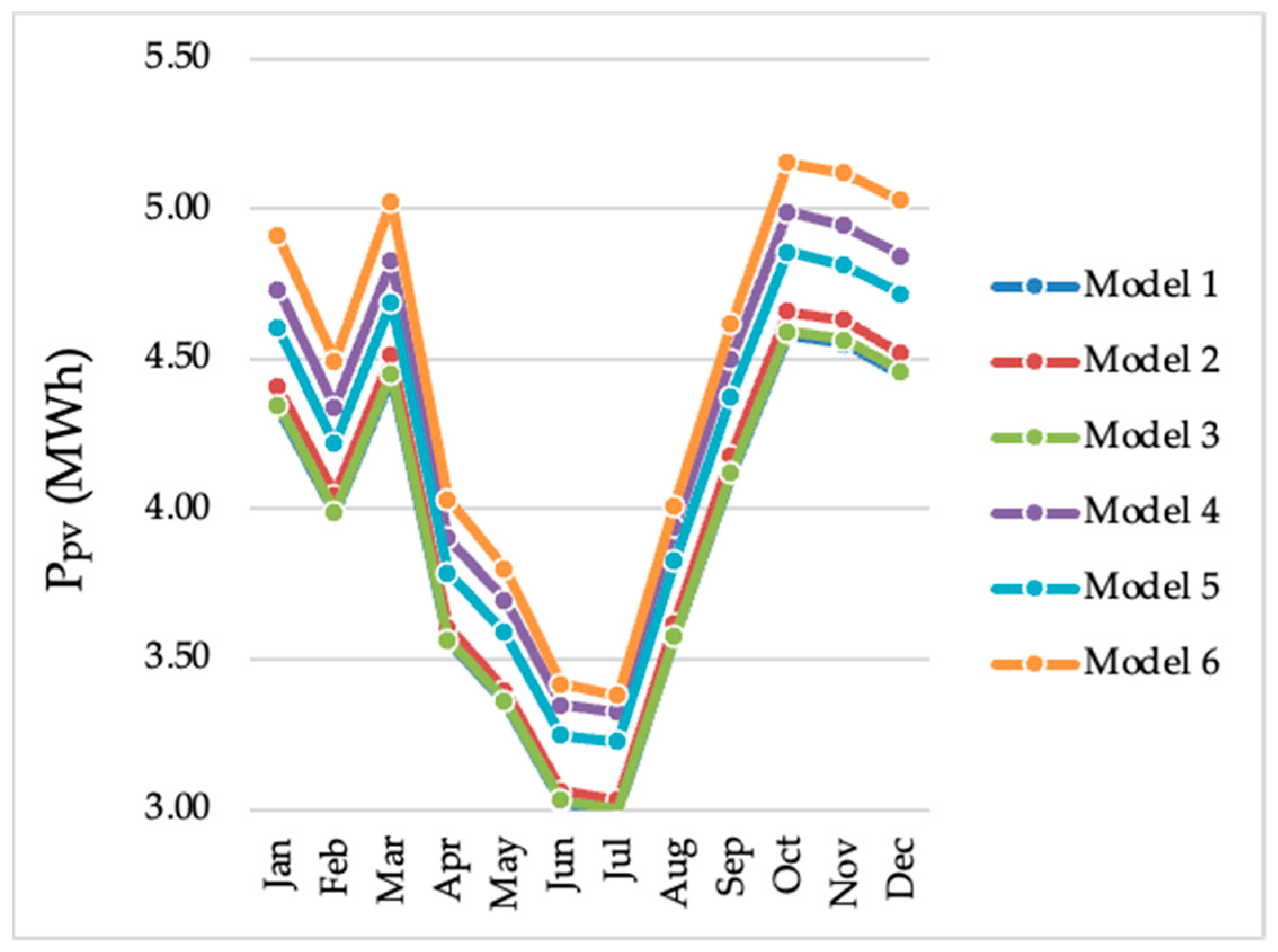
Figure 3.
values per month for the PV production calculation models in the city of João Pessoa, PB, Brazil, between the years 1961 and 2021 for 100 Axitec AC 260P/156-60S PV modules.
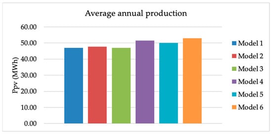
Figure 4.
Average annual values for PV production calculation models in the city of João Pessoa, PB, Brazil, between the years 1961 and 2021 for 100 Axitec AC 260P/156-60S PV modules.
As for cell temperature (Figure 1), it can be observed that, although all models have the same objective of estimating the temperature of the cells of the photovoltaic module chosen, the values are all different, despite having started from the same initial data (meteorological variables).
In Table 5, crucial information can be extracted for a better understanding of the variability of the estimated values for cell temperature. The outputs of the M5 model are the ones with the greatest disparity, predicting values up to 25.41% higher than those estimated by the M2 model. The M5 model is the one that estimates the highest amplitudes for cell temperature, and its predominant factor is accounting for the influence of relative humidity, which is not considered by the other models.
Table 5.
Average relative difference between the PV production calculation models compared two by two in the variable.
The M1 and M3 models have the lowest average difference between the estimated values, with an average difference of only 1.33%. The M4 model has similar results to the M1, M2, and M3 models, with differences between 4.16% and 6.03%.
Regarding the operational loss factor of the photovoltaic modules caused by temperature (Figure 2), it can be observed that the M4 and M5 models have the highest magnitudes. The reduction in temperature between March and October causes to increase more significantly in the M4 and M5 models, which is not observed in the others.
Average quantitative information (Table 6) was extracted for a better understanding of the variability of the values calculated for the operational loss factor of the photovoltaic modules caused by temperature. It is important to note that, as previously reported, the relative difference between the models was accentuated in the months of lower ambient temperature. In July, the relative difference was 11.08% between M1 and M4 and 10.90% between M3 and M4, both higher than the average values identified in Table 6 (9.57% and 9.34%, respectively).
Table 6.
Average relative difference between the PV production calculation models compared two by two in the variable.
As for the potential for photovoltaic energy production (Figure 3), unlike and , the estimated monthly values have a smaller internal difference. M6 is the most optimistic model, estimating the highest values for , and M1 is the most conservative model, estimating the lowest values for .
Table 7 shows that the average relative difference between the models regarding the values of follows the same behavior previously observed for , as expected, due to the characteristic of linearity of the equation that defines it (Equation (9)). The main distinction lies in the possibility of defining values for the M6 model used by Gunderson et al. (2015) [26], which considers PV cell efficiency to be constant. Therefore, there is no equation to define cell temperature or the operational loss factor.
Table 7.
Average relative difference between the PV production calculation models compared two by two in the variable.
The average relative difference from the perspective of the average estimated between these models reaches 12.89%, taking the models M1 and M6 as references. The M1 and M3 models have the lowest average difference between the estimated values, with an average difference of 0.21%. The outputs of M1, M2, and M3 have a difference from one another of at most 1.52%.
The annual production (Figure 4) follows the same behavior as the monthly production, as expected, and the production estimated by the M6 model is 12.89% higher than that calculated by the M1 model. The six sets of equations generate different results, although they use the same database, which was expected since these equations were obtained empirically.
3.2. Sensitivity Analysis
3.2.1. Sensitivity to Change in
It was observed that, as increases, the curves of the graph for (Figure 5) move linearly upwards with the increase in temperature and downwards with its decrease.
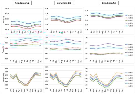
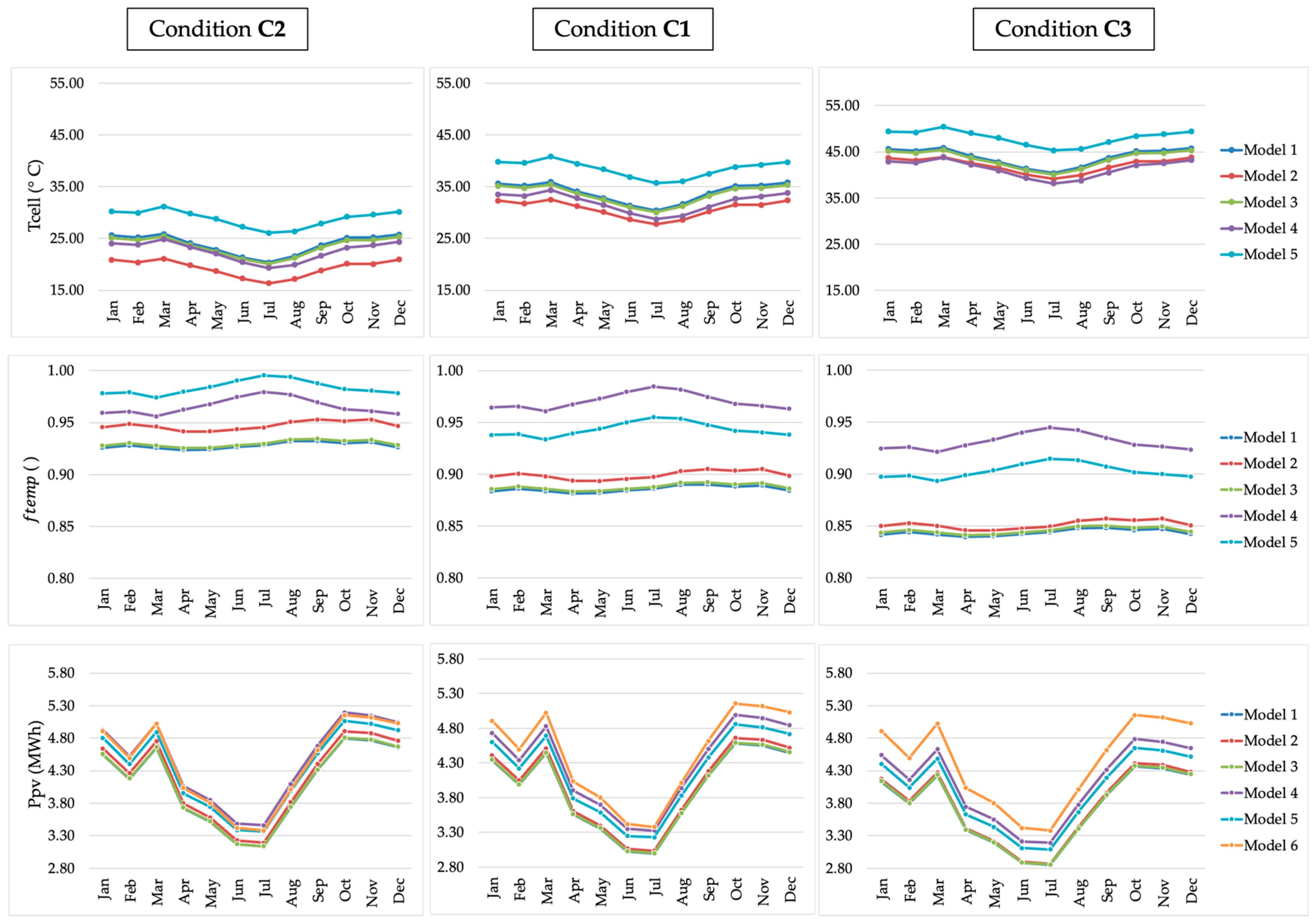
Figure 5.
Conditions to evaluate the sensitivity of the parameters to the variation of the average air temperature in each PV production calculation model.
The magnitude of these changes for conditions C1, C2, and C3 can be seen in Table 8 and Table 9. The order of magnitude of the changes relative to a specific variable can also be determined by the first-degree partial derivative of the equation that models it.
Table 8.
Average sensitivity of the variables between conditions C2 and C1 for the PV production calculation models.
Table 9.
Average sensitivity of the variables between conditions C3 and C1 for the PV production calculation models.
Due to the different sensitivities (Table 8 and Table 9), the variability between the estimated values of each model is altered when there is a change in , that is, there is a change in the dispersion of the results of the models with the variation in the ambient temperature.
The increase in causes the reduction in in M2 to be more significant than in the M1, M3, and M5 models, so that the variability between them is reduced for the climate data used.
As expected, the increase in also causes a reduction in . The increase in temperature causes the reduction in in M2 to be more significant than in the M1, M3, M4, and M5 models, so that the variability between them is changed with the increase or decrease in .
M2 is the model with the highest average sensitivity to change in for the variables , , and . The M4 model has the lowest average sensitivity for and , and the M5 model has the lowest average sensitivity for .
The primary cause of this distinction lies in the way is modeled with respect to the coefficient accounting for the influence of . While model M2 adopts a coefficient c2 of 1.14 (Equation (3)), model M4 presents a coefficient c2 of 0.961 (Equation (4)). These values will increase the estimated cell temperature more in M2 than in M4, which is why the estimated efficiency in M2 will be lower than that in M4. Moreover, model M4 also includes a term () that further reduces by considering wind speed, a term not included in the set of equations of model M2. In combination, these differences in modeling are the factors that justify the distinction between the estimated by M4 and M2 when there is a variation in . The 10 °C increase in causes reductions in of 5.32% for M2 and 4.08% for M4, an absolute difference of 1.24%.
The M6 model, because of how it was designed, has no sensitivity to temperature change and remains unchanged, while the other models have their moved upwards when temperature decreases and downwards when temperature increases.
3.2.2. Sensitivity to Change in
It was observed that the curves of the graph for (Figure 6) move linearly upwards with the increase in irradiance and downwards with its decrease. The magnitude of these changes for conditions C1, C4, and C5 can be seen in Table 10 and Table 11.
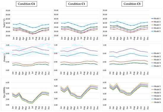
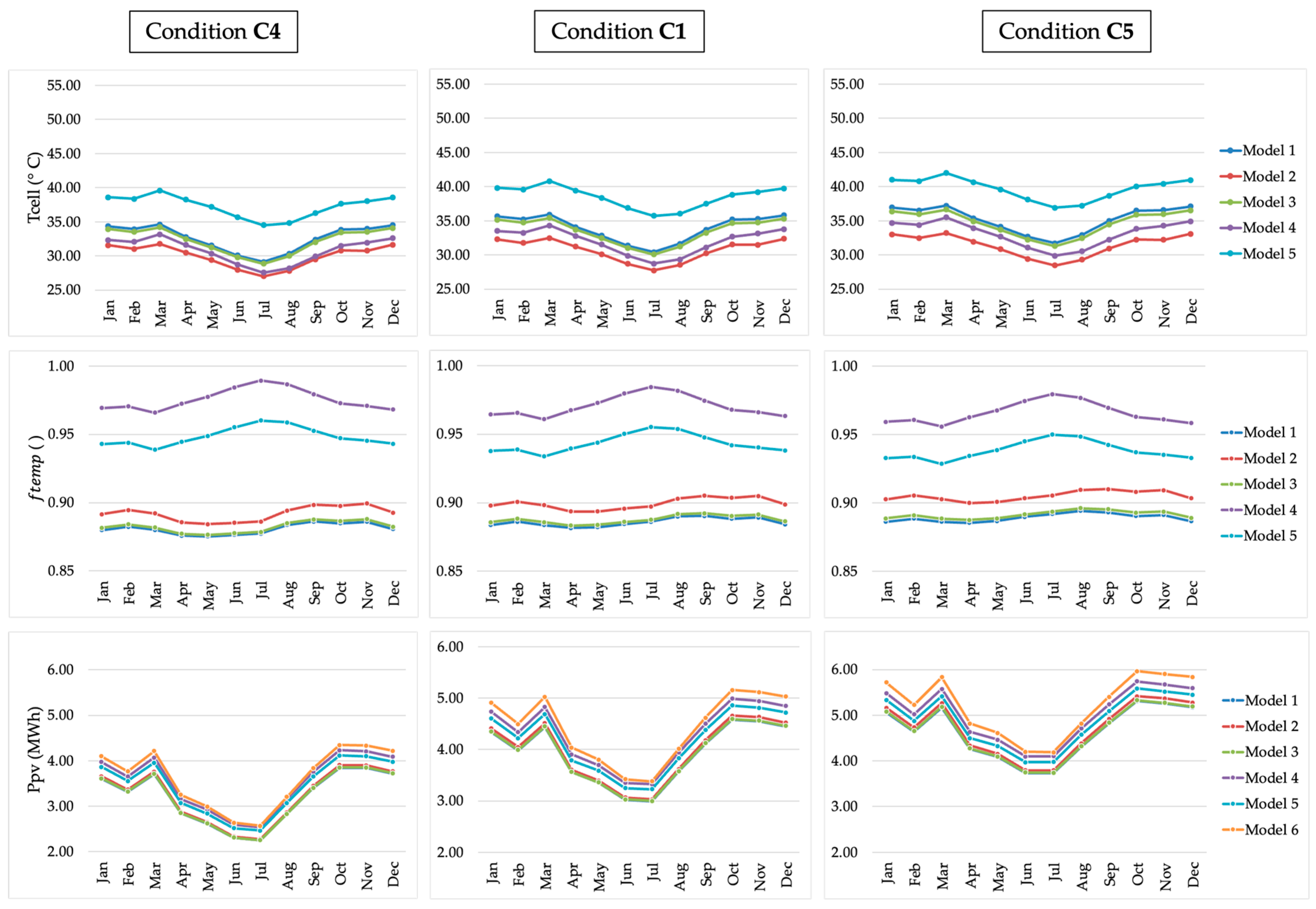
Figure 6.
Conditions to evaluate the sensitivity of the parameters to the variation of solar irradiance in each PV production calculation model.
Table 10.
Average sensitivity of the variables between conditions C4 and C1 for the PV production calculation models.
Table 11.
Average sensitivity of the variables between conditions C5 and C1 for the PV production calculation models.
As there is a change of , due to the different sensitivities (Table 10 and Table 11), the variability between the estimated values of each model is also changed when there is a change in . That is, there is a change in the dispersion of the results of the models.
The increase in caused an increase in for the M1, M2, and M3 models, and a reduction for the M4 and M5 models. These changes were minor. For M6, the variation of has influence only on .
As expected, the increase in led to an increase in , although it was responsible for the small reduction in in some of the models. The increase in irradiance causes the increase in in the M2 model to be more significant than in the M1, M3, M4, and M5 models, so that the variability between them is changed with the increase or decrease in . The M2 model has the highest sensitivity to change in for the variable, whereas the M5 model has the lowest sensitivity. The increase of 41.6667 W/m2 in causes an increase in 19.12% for the M2 model and 17.73% for the M5 model, an absolute difference of 1.39%. The increments in for all models were significant and would be plausible in cases of future reductions in local cloudiness.
3.3. Overview
When the models are analyzed, it becomes evident that the greatest similarity between them lies in the modeling of . In the six models analyzed here (M1, M2, M3, M4, M5, and M6), only two distinct equations were observed for the variable: Equations (1) and (2). The difference between these two equations is the presence of in the second equation, which quantifies the influence of irradiance. The distinction of Equation (1) lies in not considering the influence of and this causes the models that use it (M4 and M5) to be less sensitive to changes in than the others. According to Skoplaki and Palyvos (2009) [7], the -dependent term in Equation (2) serves to represent the reduction in the photovoltaic efficiency of silicon at low light levels. For , however, there is a greater divergence. When analyzing the models, it becomes evident that the biggest difference between them lies in the modeling of , since each model adopted a different way of doing it. The models M1 (Equation (6)), M2 (Equation (3)) and M3 (Equation (7)) consider the influence of only and . The authors who used these models did not justify the reason for the choice. Pérez et al. (2019) [21] found that this new linear model, M5 (Equation (4)), which additionally considers , is not suitable for wind speeds greater than 10 ms−1, as these conditions produce an unrealistically low temperature. The M4 model (Equation (5)) considers more variables, including , , , and , and pays attention to the findings of Bhattacharya et al. (2014) [42] and Kazem et al. (2012) [43], who showed that is sensitive to and also to . In a complementary way, Mekhilef et al. (2012) [44] showed two situations in which humidity can impact the performance of the PV cell: (1) the effect of water vapor particles, because the water droplets on the cell reflect solar irradiance, and (2) entry of moisture into the solar cell casing. TamizhMani et al. (2003) [23] showed that the correlation between the results of the M4 model and experimental observation is greater than 0.9. The study that used the M6 model makes it clear that the goal was to be robust by considering that the efficiency of the module does not depend on meteorological factors.
From the perspective of thermodynamics and the electrical properties of the PV cell, it is not difficult to conclude that all these meteorological parameters directly or indirectly influence cell temperature and efficiency, in view of the heat transfer mechanisms involved in this control volume. What needs to be analyzed is the precision with which these models represent reality.
Mavromatakis et al. (2014) [20] analyzed seven different relationships for , which included Equations (4) and (6) (the latter assuming an invariable wind speed of 1 m/s). They concluded that: (1) The deviations can be described by a Gaussian distribution with uncertainties similar to those of a simple heat transfer model (≈2.1–2.2 °C). It was argued that considering the simplicity of the relationships and the complexity of the thermodynamics involved, this precision is generally considered satisfactory. In addition, it was reported that a more reliable way would be to use the EN 60904-5 standard [45], but this is not easy to apply and the precision is limited by the uncertainties of various parameters.
More recently, Ozden et al. (2020) [46] compared ten distinct relationships for , which included Equations (4), (6), and (7). They concluded that models with fewer parameters—e.g., Equation (7) by Skoplaki et al. (2008) [36] and King et al. (2004) [47]—perform better than the others. This is an intriguing result since common sense would suggest that the more variables that are taken into account, the greater the expected precision. However, it should be clear that these are empirical relations that have been defined from specific situations and PV modules and, therefore, cannot represent the whole. There is a need, for example, for this type of empirical procedure to be performed under different meteorological conditions, and it is also important to consider the evaluation of the seasonal changes in PV performance.
The variability of results among the various methodologies for estimating is not something new. In 2011, Podewils (2011) [48] conducted a study with 18 software programs that estimated the of three PV plants, which showed differences of up to 20%. Such magnitude is similar to that calculated for the variability of the M6 model compared to the other models.
Roberts et al. (2017) [49] analyzed five PV models, two of which used Equation (1), and one of which used Equation (6). They also compared the performance of the models with measurements collected in a small PV plant of 2.2 kWp at OVGU University (Magdeburg, Germany), with 20 modules of 110 Wp. These authors found that the average rMBE of all power models and models based on equivalent circuits showed similar results, although with different signs: 5.14% (overestimation) and −4.91% (underestimation), respectively. These results are in line with those observed in the variability among the M1, M2, M3, and M5 models.
A great advantage of this study when comparing power models and not the already well-studied commercial software programs (RETScreen 9.0, SAM 2022.11.21, PVGIS 5.2, PVSyst 7.4, and PV*SOL 2023 ) is that the former have the ability to better estimate in a monthly frequency. González-Peña et al. (2021) [50] concluded that software programs, in global annual terms, mostly show deviations below 10%. However, this apparent good result hides poor estimates throughout the year, in which overestimates are offset by underestimates month by month. A greater error at the monthly level can create unwanted situations for the managers of PV plants, especially in terms of energy availability. González-Peña et al. (2021) [50] reported in their study a deviation of up to 31.0% in the month of November for the PV*SOL software for a fixed system.
Recently, Fuster-Palop et al. (2022) [51] compared the results obtained from a power model (using Equations (1) and (6)), a statistical model (MLR), and a machine learning model (RF) for a PV plant in the west of Olmedilla de Alarcón (Cuenca, Spain) of 60 MWp. This plant is the largest so far analyzed based on the performance reported in the literature. The power model showed point errors greater than 5%, but an annual error of 1.81%, in line with what was observed in this study. They concluded that both statistical models provided better precision than the power model. However, their use is conditioned on the availability of measured data from the PV plant, which is not possible in the planning phase, before the plant goes into operation.
Morais et al. (2021) [52] conducted a study with a PV plant of IFPI at the campus of Floriano (Piauí, Brazil) of 171.6 kWp, with 660 modules of 260 Wp. The authors used three solar irradiation databases (INMET, SWERAS, and ABES) together with a methodology similar to that of the M6 model, and two software programs (Pvsyst and Solergo 2023) to compare estimates of electricity generation. Morais et al. (2021) [52] concluded that the choice of methodology for calculating estimates can directly influence the results of economic feasibility analyses. Investments are made based on, among several factors, the internal rate of return (IRR), and the authors showed that under one methodology the IRR would be −0.87%, while under the other it would be 2.52%. That is, one indicates loss and the other indicates profit. Given this situation, it is easy to visualize the possible impacts derived from errors of estimates and, therefore, the importance of knowing the most conservative and optimistic power models.
It is common to associate the impacts derived from errors of estimates only with PV plants; however, it should be clear that the range is much greater, being linked to any system that uses photovoltaic energy. Silva et al. (2018) [53], for example, conducted a study analyzing the feasibility of producing energy for electric vehicles using a PV structure of 1.26 kWp. These authors concluded that only one of seventeen models of electric vehicles could be powered exclusively by the energy from this structure. The remaining question was: ‘is this estimate conservative, optimistic or average compared to the other methodologies used?’ The present study helps create parameters by starting a line of research that seeks to compare existing and exhaustively used power models in the literature in addition to initiated research, such as that of Correa-Betanzo et al. (2018) [54], who analyzed the impact on according to the model adopted for .
4. Conclusions
Different sets of equations are used to estimate photovoltaic energy production (). It turns out that there is a gap in how distinct the outputs of these models are. This study established the most used sets of equations in the literature to estimate the potential of photovoltaic energy production from meteorological variables. In addition, it analyzed the variability and sensitivity of these sets of equations when there is variation in climatic conditions.
In the literature, six models were identified to estimate and all of them were analyzed from the perspective of variability and sensitivity. Model M1 [24,29] uses ambient temperature and nominal operating cell temperature, along with solar irradiance, to estimate . Model M2 [3,15,27,33,34,35] employs the same inputs as M1 but excludes nominal operating cell temperature when estimating . Model M3 [25] continues with these inputs from M2 but introduces different coefficients to account for variable influences in calculation. Model M4 [22] retains the same parameters as M2, now also incorporating the direct impact of wind speed. Model M5 [2,3,21,38] utilizes the same variables as M4, additionally incorporating the direct influence of air humidity. Model M6 [26] simplifies the approach, considering that depends solely on solar irradiance, ensuring that changes in meteorological variables do not affect the efficiency of the photovoltaic module, distinguishing it from the previous five models.
Under the climatic conditions of the city of João Pessoa (Paraíba, Brazil), the M6 model is the most optimistic, estimating the highest values for . The M1 model is the most conservative, estimating the lowest values for . The estimated annual difference in between these models reaches 12.89%. Note that, according to percentage difference analysis, the variation in results varies depending on the climatic data, causing dispersion between models to be affected. The sensitivity analyses showed that, due to the different sensitivities, the variability among the models is altered with the change of and with the change of . Therefore, similar studies in different climatic conditions are recommended.
Regarding sensitivity to changes in meteorological variables, models M1, M2, M3, M4, and M5 have their estimated moved upwards when temperature decreases and downwards when temperature increases, as expected. The M6 model is an exception. Due to its design, this model is not sensitive to temperature changes and remains unchanged when changes. The M2 model has the highest sensitivity to change in for the variable, while M5 has the lowest sensitivity. The increase of 41.6667 W/m2 in causes an increase in of 19.12% for the M2 model and 17.73% for the M5 model, a relative difference of 7.84%. Under the changes in , the 10 °C increase in causes a reduction in of 5.32% for the M2 model and 4.08% for the M4 model, a relative difference of 30.39%.
The importance of determining the variability and sensitivity of the main sets of equations used in the literature to estimate the potential of photovoltaic energy production from meteorological variables has been highlighted. The outputs of the analyzed models show distinctions and sensitivities that can significantly influence the conclusions of studies in this research area. The variations and sensitivities observed among the models are so significant that they can influence conclusions in studies aiming to predict photovoltaic energy trends in specific regions. As tendencies are analyzed, it is crucial to consider their implications in feasibility analyses. These divergences can, in turn, re-formulate feasibility analyses and compromise the reliability of photovoltaic energy systems, thus leading to economic and socio-environmental changes.
Author Contributions
Conceptualization, N.M.F.T.S.A. and R.A.; Methodology, N.M.F.T.S.A. and S.E.L.M.; Validation, N.M.F.T.S.A., S.E.L.M. and R.A.; Formal analysis, N.M.F.T.S.A.; Investigation, N.M.F.T.S.A.; Writing—original draft, N.M.F.T.S.A.; Writing—review & editing, R.A. All authors have read and agreed to the published version of the manuscript.
Funding
The present study was carried out with support from the Brazilian National Council for Scientific and Technological Development (CNPq) (project 308753/2021-6), the Paraíba State Research Foundation (FAPESQ) (Project 3063/2021 and Grant 18/2020) and PROPESQ/UFPB (project PVK13163-2020).
Data Availability Statement
The data presented in this study are available on request from the corresponding author.
Conflicts of Interest
The authors declare no conflict of interest. The funders had no role in the design of the study; in the collection, analyses, or interpretation of data; in the writing of the manuscript; or in the decision to publish the results.
References
- Feron, S.; Cordero, R.R.; Labbe, F. Rural electrification efforts based on off-grid photovoltaic systems in the Andean region: Comparative assessment of their sustainability. Sustainability 2017, 9, 1825. [Google Scholar] [CrossRef]
- Feron, S.; Cordero, R.R.; Damiani, A.; Jackson, R.B. Climate change extremes and photovoltaic power output. Nat. Sustain. 2021, 4, 270–276. [Google Scholar] [CrossRef]
- Jerez, S.; Tobin, I.; Vautard, R.; Montavez, J.P.; Lopez-Romero, J.M.; Thais, F.; Bartok, B.; Christensen, O.B.; Colette, A.; Deque, M.; et al. The impact of climate change on photovoltaic power generation in Europe. Nat. Commun. 2015, 6, 10014. [Google Scholar] [CrossRef]
- Kafka, J.L.; Miller, M.A. A climatology of solar irradiance and its controls across the United States: Implications for solar panel orientation. Renew. Energy 2019, 135, 897–907. [Google Scholar] [CrossRef]
- Zuluaga, C.F.; Avila-Diaz, A.; Justino, F.B.; Martins, F.R.; Ceron, W.L. The climate change perspective of photovoltaic power potential in Brazil. Renew. Energy 2022, 193, 1019–1031. [Google Scholar] [CrossRef]
- Zhang, J.; You, Q.; Ullah, S. Changes in photovoltaic potential over China in a warmer future. Environ. Res. Lett. 2022, 17, 114032. [Google Scholar] [CrossRef]
- Niu, J.; Qin, W.; Wang, L.; Zhang, M.; Wu, J.; Zhang, Y. Climate change impact on photovoltaic power potential in China based on CMIP6 models. Sci. Total Environ. 2023, 858, 159776. [Google Scholar] [CrossRef]
- Ha, S.; Zhou, Z.; Im, E.; Lee, Y. Comparative assessment of future solar power potential based on CMIP5 and CMIP6 multi-model ensembles. Renew. Energy 2023, 206, 324–335. [Google Scholar] [CrossRef]
- Klise, G.T.; Stein, J.S. Models Used to Assess the Performance of Photovoltaic Systems; Sandia National Laboratories (SNL): Albuquerque, NM, USA, 2009. [Google Scholar]
- Djamila, M.; Ernest, R. Modeling of solar irradiance and cells. In Optimization of Photovoltaic Power Systems: Modelization, Simulation and Control; Springer-Verlag London Ltd.: London, UK, 2012; pp. 31–87. [Google Scholar]
- Skoplaki, E.; Palyvos, J.A. On the temperature dependence of photovoltaic module electrical performance: A review of efficiency/power correlations. Sol. Energy 2009, 83, 614–624. [Google Scholar] [CrossRef]
- Zondag, H.A. Flat-plate PV-Thermal collectors and systems: A review. Renew. Sustain. Energy Rev. 2008, 12, 891–959. [Google Scholar] [CrossRef]
- Evans, D.L. Simplified method for predicting photovoltaic array output. Sol. Energy 1981, 27, 555–560. [Google Scholar] [CrossRef]
- Tonui, J.K.; Tripanagnostopoulos, Y. Performance improvement of PV/T solar collectors with natural air flow operation. Sol. Energy 2008, 82, 1–12. [Google Scholar] [CrossRef]
- Crook, J.A.; Jone, L.A.; Forster, P.M.; Crook, R. Climate change impacts on future photovoltaic and concentrated solar power energy output. Energy Environ. Sci. 2011, 4, 3101–3109. [Google Scholar] [CrossRef]
- Duffie, J.A.; Beckman, W.A. Solar Energy Thermal Processes, 3rd ed.; Wiley: Hoboken, NJ, USA, 2006. [Google Scholar]
- Kou, Q.; Klein, S.A.; Beckman, W.A. A method for estimating the long-term performance of direct-coupled PV pumping systems. Sol. Energy 1998, 64, 33–40. [Google Scholar] [CrossRef]
- Lasnier, F.; Ang, T.G. Photovoltaic Engineering Handbook, 1st ed.; Adam Hilger: New York, NY, USA, 1990; 572p. [Google Scholar]
- Chenni, R.; Makhlouf, M.; Kerbache, T.; Bouzid, A. A detailed modeling method for photovoltaic cells. Energy 2007, 32, 1724–1730. [Google Scholar] [CrossRef]
- Mavromatakis, F.; Kavoussanaki, E.; Vignola, F.; Franghiadakis, Y. Measuring and estimating the temperature of photovoltaic modules. Sol. Energy 2014, 110, 656–666. [Google Scholar] [CrossRef]
- Pérez, J.C.; González, A.; Díaz, J.P.; Expósito, F.J.; Felipe, J. Climate change impact on future photovoltaic resource potential in an orographically complex archipelago, the Canary Islands. Renew. Energy 2019, 133, 749–759. [Google Scholar] [CrossRef]
- Sawadogo, W.; Abiodun, B.J.; Okogbue, E.C. Impacts of global warming on photovoltaic power generation over West Africa. Renew. Energy 2020, 151, 263–277. [Google Scholar] [CrossRef]
- Tamizhmani, G.; Ji, L.; Tang, Y.; Petacci, L.; Osterwald, C. Photovoltaic module thermal/wind performance: Long-term monitoring and model development for energy rating. In Proceedings of the NCPV and Solar Program Review Meeting, Denver, CO, USA, 24–26 March 2003; Volume 1, pp. 936–939. [Google Scholar]
- Zou, L.; Wang, L.; Li, J.; Lu, Y.; Gong, W.; Niu, Y. Global surface solar radiation and photovoltaic power from coupled model intercomparison project phase 5 climate models. J. Clean. Prod. 2019, 224, 304–324. [Google Scholar] [CrossRef]
- Smith, C.J.; Crook, J.A.; Crook, R.; Jackson, L.S.; Osprey, S.M.; Forster, P.M. Impacts of Stratospheric Sulfate Geoengineering on Global Solar Photovoltaic and Concentrating Solar Power Resource. J. Appl. Meteorol. Climatol. 2017, 56, 1483–1497. [Google Scholar] [CrossRef]
- Gunderson, I.; Goyette, F.; Gago-Silva, A.; Quiquerez, L.; Lehmann, A. Climate and land-use change impacts on potential solar photovoltaic power generation in the Black Sea region. Environ. Sci. Policy 2015, 46, 70–81. [Google Scholar] [CrossRef]
- Bazyomo, S.D.Y.B.; Lawin, E.A.; Coulibaly, O.; Ouedraogo, A. Forecasted Changes in West Africa Photovoltaic Energy Output by 2045. Climate 2016, 4, 53. [Google Scholar] [CrossRef]
- Perpiñán, O. solaR: Solar Radiation and photovoltaic Systems with R. J. Stat. Softw. 2012, 50, 1–32. [Google Scholar] [CrossRef]
- Medeiros, S.E.L.; Nilo, P.F.; Silva, L.P.; Santos, C.A.C.; Carvalho, M.; Abrahão, R. Influence of climatic variability on the electricity generation potential by renewable sources in the Brazilian semi-arid region. J. Arid. Environ. 2021, 184, 104331. [Google Scholar] [CrossRef]
- Evans, D.L.; Florschuetz, L.W. Cost studies on terrestrial photovoltaic power systems with sunlight concentration. Sol. Energy 1977, 19, 255–262. [Google Scholar] [CrossRef]
- Spectrolab. Photovoltaic Systems Concept Study; Rep. AL0-2748-12; Spectrolab, Inc.: Sylmar, CA, USA, 1977. [Google Scholar]
- Ross, R.G.; Smokler, M.I. Flat-Plate Solar Array Project Final Report—Vol. VI: Engineering Sciences and Reliability; Report DOE/JPL-1012-125; Jet Propulsion Lab.: Pasadena, CA, USA, 1986. [Google Scholar]
- Zhao, X.; Huang, G.; Lu, C.; Zhou, X.; Li, Y. Impacts of climate change on photovoltaic energy potential: A case study of China. Appl. Energy 2020, 280, 115888. [Google Scholar] [CrossRef]
- Panagea, I.S.; Tsanis, I.K.; Koutroulis, A.G.; Grillakis, M.G. Climate change impact on photovoltaic energy output: The case of Greece. Adv. Meteorol. 2014, 2014, 264506. [Google Scholar] [CrossRef]
- Wild, M.; Folini, D.; Henschel, F.; Fischer, N.; Müller, B. Projections of long-term changes in solar radiation based on CMIP5 climate models and their influence on energy yields of photovoltaic systems. Sol. Energy 2015, 116, 12–24. [Google Scholar] [CrossRef]
- Skoplaki, E.; Boudouvis, A.G.; Palyvos, J.A. A simple correlation for the operating temperature of photovoltaic modules of arbitrary mounting. Sol. Energy Mater. Sol. Cells 2008, 92, 1393–1402. [Google Scholar] [CrossRef]
- Lewis, C.A.; Kirkpatric, J.P. Solar cell characteristics at high solar intensities and temperatures. In Proceedings of the 8th IEEE Photovoltaic Specialists Conference Record, Seattle, WA, USA, 4–6 August 1970; pp. 123–134. [Google Scholar]
- Bichet, A.; Hingray, B.; Evin, G.; Diedhiou, A.; Kebe, C.M.F.; Anquetin, S. Potential impact of climate change on solar resource in Africa for photovoltaic energy: Analyses from CORDEX-AFRICA climate experiments. Environ. Res. Lett. 2019, 14, 124039. [Google Scholar] [CrossRef]
- Sorensen, B. GIS management of solar resource data. Sol. Energy Mater. Sol. Cells 2001, 67, 503–509. [Google Scholar] [CrossRef]
- Axitec. AXI Power: 60-Cell Polycrystalline Solar Module. 2016. Available online: https://www.axitecsolar.com/solarmodule-von-axitec (accessed on 24 January 2022).
- Notton, G.; Cristofari, C.; Mattei, M.; Poggi, P. Modelling of a double-glass photovoltaic module using finite differences. Appl. Therm. Eng. 2005, 25, 2854–2877. [Google Scholar] [CrossRef]
- Bhattacharya, T.; Chakraborty, A.K.; Pal, K. Effects of ambient temperature and wind speed on performance of monocrystalline solar photovoltaic module in Tripura. India J. Sol. Energy 2014, 2014, 817078. [Google Scholar] [CrossRef]
- Kazem, H.A.; Chaichan, M.T.; Al-Shezawi, I.M.; Al-Saidi, H.S.; Al-Rubkhi, H.S.; Alsinani, K.; Al-Waeli, A.H.A. Effect of Humidity on the PV Performance in Oman. Asian Trans. Eng. 2012, 2, 29–32. [Google Scholar]
- Mekhilef, S.; Saidur, R.; Kamalisarvestani, M. Effect of dust, humidity and air velocity on efficiency of photovoltaic cells. Renew. Sustain. Energy Rev. 2012, 16, 2920–2925. [Google Scholar] [CrossRef]
- EN 60904-5; Photovoltaic Devices–Part 5: Determination of the Equivalent Cell Temperature (ECT) of Photovoltaic (PV) Devices by the Open-Circuit Method. iTeh, Inc.: Newark, DE, USA, 1995.
- Orzen, T.; Tolgay, D.; Yakut, M.S.; Akinoglu, B.G. An extended analysis of the models to estimate photovoltaic module temperature. Turk. J. Eng. 2020, 4, 183–196. [Google Scholar]
- King, D.L.; Boyson, W.E.; Kratochvil, J.A. Photovoltaic Array Performance Model; No: SAND2004-3; Sandia National Laboratories: Springfield, VA, USA, 2004. [Google Scholar]
- Podewils, C. Differenze evidenti. Quel che i gestori degli impianti dovrebbero sapere sui programmi di simulazione. Photon 2011, 5, 140–147. [Google Scholar]
- Roberts, J.J.; Zevallos, A.A.M.; Cassula, A.M. Assessment of photovoltaic performance models for system simulation. Renew. Sustain. Energy Rev. 2017, 72, 1104–1123. [Google Scholar] [CrossRef]
- González-Peña, D.; García-Ruiz, I.; Díez-Mediavilla, M.; Dieste-Velasco, M.I.; Alonso-Tristán, C. Photovoltaic Prediction Software: Evaluation with Real Data from Northern Spain. Appl. Sci. 2021, 11, 5025. [Google Scholar] [CrossRef]
- Fuster-Palop, E.; Vargas-Salgado, C.; Ferri-Revert, J.C.; Payá, J. Performance analysis and modelling of a 50 MW grid-connected photovoltaic plant in Spain after 12 years of operation. Renew. Sustain. Energy Rev. 2022, 170, 112968. [Google Scholar] [CrossRef]
- Morais, F.H.M.; Oliveira, O.A.V.; Silva, L.; Moraes, A.M.; Barbosa, F.R. Influência da Irradiação Solar na Análise de Viabilidade Econômica de Sistemas Fotovoltaicos. Rev. Bras. Meteorol. 2021, 36, 723–734. [Google Scholar] [CrossRef]
- Silva, J.E.; Santos, F.R.; Kaltmaier, G.; Urbanetz Junior, J. Implementation of a photovoltaic panel to supply electric cars energy demands. Braz. Arch. Biol. Technol. 2018, 61, e18000530. [Google Scholar] [CrossRef]
- Correa-Betanzo, C.; Calleja, H.; León-Aldaco, S. Module temperature models assessment of photovoltaic seasonal energy yield. Sustain. Energy Technol. Assess. 2018, 27, 9–16. [Google Scholar] [CrossRef]

Disclaimer/Publisher’s Note: The statements, opinions and data contained in all publications are solely those of the individual author(s) and contributor(s) and not of MDPI and/or the editor(s). MDPI and/or the editor(s) disclaim responsibility for any injury to people or property resulting from any ideas, methods, instructions or products referred to in the content. |
© 2024 by the authors. Licensee MDPI, Basel, Switzerland. This article is an open access article distributed under the terms and conditions of the Creative Commons Attribution (CC BY) license (https://creativecommons.org/licenses/by/4.0/).