Investigation of Wall Boiling Closure, Momentum Closure and Population Balance Models for Refrigerant Gas–Liquid Subcooled Boiling Flow in a Vertical Pipe Using a Two-Fluid Eulerian CFD Model

Abstract

The precise design of heat exchangers in automobile air conditioning systems for more sustainable electric vehicles requires an enhanced assessment of CFD mechanistic models for the subcooled boiling flow of pure eco-friendly refrigerant. Computational Multiphase Flow Dynamics (CMFDs) relies on two-phase closure models to accurately depict the complex physical phenomena involved in flow boiling. This paper thoroughly examines two-phase CMFD flow boiling, incorporating sensitivity analyses of critical parameters such as boiling closures, momentum closures, and population balance models. Three datasets from the DEBORA experiment, involving vertical pipes with subcooled boiling flow of refrigerant at three different pressures and varying levels of inlet liquid subcooling, are used for comparison with CFD simulations. This study integrates nucleate site density and bubble departure diameter models to enhance wall boiling model accuracy. It aims to investigate various interfacial forces and examines the S-Gamma and Adaptive Multiple Size-Group (A-MuSiG) size distribution methods for their roles in bubble break up and coalescence. These proposed approaches demonstrate their efficacy, contributing to a deeper understanding of flow boiling phenomena and the development of more accurate models. This investigation offers valuable insights into selecting the most appropriate sub-closure models for both boiling closure and momentum closure in simulating boiling flows.

1. Introduction

Two-phase technologies, widely utilized in the energy sector, offer numerous benefits such as precise temperature control, broad heat transport capacity, diode functionality, temperature uniformity and adaptable design, thus presenting reliable solutions [1]. Modeling two-phase flows such as boiling flows is complicated due to their complex nature, making it difficult to formulate constitutive equations that can accurately represent various flow patterns. This complexity further challenges the use of these models in designing electronic cooling applications as well as large scale nuclear reactors. Computational methods were extensively applied to analyze flow boiling using Eulerian methods, and these examples include the nucleate pool boiling of a single bubble [2,3] saturated flow boiling in the micro-channel [4,5] and the interfacial phenomena of specific flow regimes [6]. In the Eulerian–Eulerian approach, the conservation equations of mass, momentum, and energy are solved for each phase separately. The transfer of mass, momentum, and heat energy between phases is modeled through interfacial terms within these equations.

However, the interface structure information is lost in this model as the averaged probability of occurrence for each phase in time and space is used. Various wall boiling models were implemented in advanced Computational Fluid Dynamic (CFD) codes to predict the boiling process. Wall-boiling models have indeed been developed to simulate boiling phenomena near a heated wall, where the rates of heat and mass transfer are calculated. In the context of two-fluid averaged models, the prevailing methods heavily rely on the Rensselaer Polytechnic Institute (RPI) boiling model developed by Kurul and Podowski [7]. The heat flux originating from the wall is allocated among various mechanisms governing the heat transfer process, including single-phase convection, quenching, and evaporation.

Over the past few years, numerous authors have employed varying degrees of refinement within the Rensselaer Polytechnic Institute (RPI) boiling model to anticipate boiling flows [8,9,10,11,12,13,14]. Through the advancement and implementation of numerical methods that couple two-fluid and wall boiling models, the use of bubble dynamic models becomes necessary as they offer fundamental parameters crucial for solving wall heat flux partitioning models [15]. The process of bubble growth entails significant heat exchange due to vaporization. Hence, the nucleation density, which determines the number of growing bubbles along with related dynamic parameters governing bubble growth, contributes to comprehending flow boiling and its related improved heat transfer performance. Till now accurate predictions of the heat transfer coefficient and Departure from Nucleate Boiling (DNB) remain challenging due to the reliance on empirical correlations within the RPI model and its inherent limitations.

As bubbles grow to a specific size, changes in force characteristics prompt their departure from the nucleation site, leading them to either slide on or detach from the heated wall, accompanied by heat exchange. Yet, the local heat transfer and mechanical attributes of bubbles exhibit randomness, presenting considerable challenges for related research endeavors. Consequently, statistical correlations depicting key parameters of bubble dynamics hold greater value in industrial applications and simulation analyses. In addition to wall boiling, accurate calculation of interphase momentum transfer between phases in flow boiling is essential for predicting overall boiling flow. Amid various closure models, those specifically addressing interfacial forces wield substantial influence on the precision of CFD predictions [16,17,18]. Modeling turbulent bubbly flow presents challenges owing to the intricate nature of interactions among hydrodynamic forces, bubble coalescence and break-up mechanisms. Given the lack of flawless closure models for these interfacial forces, it is of utmost significance to meticulously choose the simulation parameters associated with these forces.

Upon reviewing interfacial forces, it becomes evident that they play a pivotal role in multiphase CFD. However, there is no universally established method available in the open literature for selecting these forces [19]. Two-fluid solvers commonly assume a uniformly dispersed phase in multiphase flow modeling, assuming particles are of the same size [20]. This simplification allows for an effective representation of key flow characteristics. While this approach proves robust for numerous applications, it becomes inadequate when dealing with varying particle sizes due to different physical processes in multiphase flows. This limitation can be addressed by incorporating additional population balance equations (PBEs) to conserve internal properties like particle number, mass, or volume, overcoming the constraints associated with assuming a constant particle size [21]. Bubble growth is modeled by coupling with a population balance model (PBM) which accounts for interactions such as bubble break up and coalescence, leading to a non-uniform bubble size distribution that aids in the development of flow regimes. In recent developments, the prediction of bubble size distribution has involved the integration of various population balance methods with both the two-fluid and wall boiling models. One advantage of using PBM is the ability to determine bubble size in terms of the Sauter diameter, a parameter commonly evaluated in experiments. The investigation by Hu et al. [22] highlighted the importance of adjusting coalescence and breakage factors within PBM sub-models to align with experimental data for achieving reasonable results.

Within the bubble column, there exists a dynamic interaction between the gas dispersed within the liquid, influencing the interphase forces and turbulence within the column. Therefore, achieving an accurate solution for bubble columns depends on the precise modeling of interphase forces and turbulence models [23,24,25]. Nevertheless, the accuracy of CFD code is constrained by the appropriate choice of suitable closure expressions governing interphase mass, momentum and heat exchange between two phases, encompassing both the dispersed and continuous phases [26,27]. Presently, a variety of closure models are found in the literature, based on experimental, analytical and computational methods.

Most of the boiling models were tested against water-vapor experimental measurements made in subcooled boiling flows. The majority of boiling models have undergone validation through comparisons with experimental measurements conducted in subcooled boiling flows. Most of these experiments were conducted using circular cross-sectional geometries, employing water at low pressure [28] or refrigerant at moderate pressure [29,30,31], as they mirror the typical operating conditions observed in water-cooled nuclear reactors. Cheung et al. [32] conducted a comprehensive review of numerous formulations and quantitatively evaluated their suitability for subcooled flow boiling under low-pressure conditions, concluding that no single combination could consistently yield reliable results across a wide range of test cases. The work of Murallidharan et al. [33] provided an in-depth understanding of the functioning of the wall heat flux partitioning (WHFP) model and how its correlations can affect its predictability. Krepper et al. [34] conducted simulations on water-vapor experimental data by Bartolomei and Chanturiya [35] and highlighted the significance of the models utilized for boiling and momentum closures. A complete analysis of bubble departure diameter and frequency correlations was offered in the work of Brooks and Hibiki [36], highlighting that the available models show large errors when compared to the available experimental datasets of vertical upward flow, vertical downward flow and horizontal flow, including different working fluids and a wide range of flow conditions from the literature. Within the domain of CFD, notable correlations utilized include those developed by Lemmert and Chawla [37], Hibiki and Ishii [38] for active nucleation site density, Tolubinsky and Kostanchuk [39] and Kocamustafaogullari [40] for bubble departure diameter, and Cole [41] for bubble departure frequency [9,10,12,14,42]. Cong et al. [43] discussed that, regarding the wall boiling model and interfacial exchange models, there are a large number of coefficients used to model the subcooled boiling flow. In their work, the authors predicted a subcooled boiling flow with a two-phase CFD code, considering the uncertainties caused by the model parameters, including models for inter-phase exchange and for boiling processes at the heated wall. Q. Wang and W. Yao [44] conducted a comprehensive study to evaluate the accuracy and differences in interphase force models used in bubbly flow simulations for an isothermal air–water system. For the purpose of modeling validation, they selected three experimental cases of bubbly flow, each characterized by a wide range of Reynolds numbers at the inlet. Their findings indicate that the choice of correlations for drag force, lift force, and wall lubrication force should be made with careful consideration of the Reynolds numbers range. Additionally, they observed that the selection of turbulence models and turbulence dispersion force models has a minimal impact on the simulation outcomes. J. Gu et al. [45] performed detailed numerical simulations of water-vapor two-phase flow under ultra-high-pressure conditions to predict subcooled boiling flow in a vertical heated tube. These simulations employed an extended RPI wall boiling model. To ensure the accuracy of the closure model, the numerical results were rigorously validated against experimental data provided by Bartolemei et al. [35,46]. The experiments measured the subcooled boiling parameters of water-vapor two-phase flow in a vertical circular tube with an inner diameter of 15.4 mm. Conducted under operating conditions relevant to high-pressure nuclear applications, these experiments offered a robust benchmark for validating the numerical model. G. S. Gray and S. J. Ormiston [47] investigated the performance of a two-fluid model using the commercial CFD software ANSYS CFX (Version 2020-R1). Their study aimed to predict the characteristics of the upward isothermal bubbly flow of air and water in a vertical pipe. The findings indicated that the predictive accuracy of the two-fluid CFD model is critically dependent on the precision of the implemented closure models. Yang et al. [48] conducted an in-depth experimental examination of two-phase refrigerant flow under various conditions to assess how different refrigerant liquids impact system performances. Their study revealed that the properties of the fluids, the flow conditions, and the resulting flow patterns significantly affect both pressure drops and heat transfer coefficients during flow boiling. Consequently, it is crucial for the reliable CMFD-based design of air conditioning heat exchangers to rigorously validate closure models for refrigerant flow boiling. This ensures that these sub-models are accurately represented.

The preceding discussion underscores the absence of a universally accepted methodology regarding boiling and momentum closures within the domain of fluid dynamics. This discrepancy primarily stems from the scarcity of experimental and empirical data on crucial parameters like bubble departure diameter, departure frequency and nucleation site densities. This lack is especially significant in the context of refrigerant flow. Of particular significance is the precise prediction of radial void fraction, a fundamental requirement for accurately simulating Departure from Nucleate Boiling (DNB), especially in close proximity to the walls. A detailed comparison of CMFD results in the context of refrigerant flow is crucial because the distribution of radial voids is profoundly influenced by various forces. These include both drag forces and non-drag forces such as wall lubrication, lift and turbulent dispersion forces. It is essential to understand which forces to include or exclude when using the two-fluid approach. Including certain forces may lead to numerical divergence issues while excluding others can result in unrealistic solutions due to unsuitable momentum closure models. Recently, numerous developments have been made to improve the accuracy of two-fluid Eulerian approaches in CMFDs. This approach of flow boiling, utilizing mechanistic models, holds significant interest due to its applicability in various industrial scenarios, such as refrigerant boiling flow. However, the proper application of different closure models presents significant challenges, and the existing literature lacks practical comparisons with experimental data, particularly in the context of subcooled boiling flow with refrigerants.

The present comprehensive investigation aims to conduct a sensitivity analysis including three critical parameters newly proposed in commercial codes—wall boiling closures, momentum closure and the population balance model—for refrigerant boiling flow in vertical pipes, thereby filling a lack in the scientific literature. The present investigation also assesses the influence of grid size and involves the practical implementation of these models, as well as evaluating the combined effects of the models and their sub-models.

The comprehensive study is made for subcooled boiling refrigerant flow as this case is of primary importance for the design of phase-change heat exchangers such as those of automobile air conditioning systems. The DEBORA experiment, conducted by Garnier et al. [30,49], serves as a comprehensive benchmark with a wide range of operating parameter variations (pressure, inlet subcooling) and extensive results for several parameters, facilitating the validation of numerical approaches. This experiment provides local measurements of the flow boiling of a coolant refrigerant. A notable feature of the DEBORA experiment is its simple geometry, which can be approximated with an axisymmetric-2D model. Unlike average bulk measurements, the DEBORA experiment offers local distributions at the outlet, providing essential data for validating CFD models and enhancing the understanding of heat transfer and phase change phenomena. Three datasets from the DEBORA experiment, involving vertical pipes with subcooled boiling flow of refrigerant R12 at three different pressures and varying levels of inlet liquid subcooling, are used for comparison with the present CFD simulations.

The principal objective of this paper is then to assess the effectiveness of the two-fluid model in conjunction with a wall partitioning model, while simultaneously evaluating the efficacy of different closure models for wall boiling, momentum forces, and population balance models (PBM) within the framework of a refrigerant configuration system.

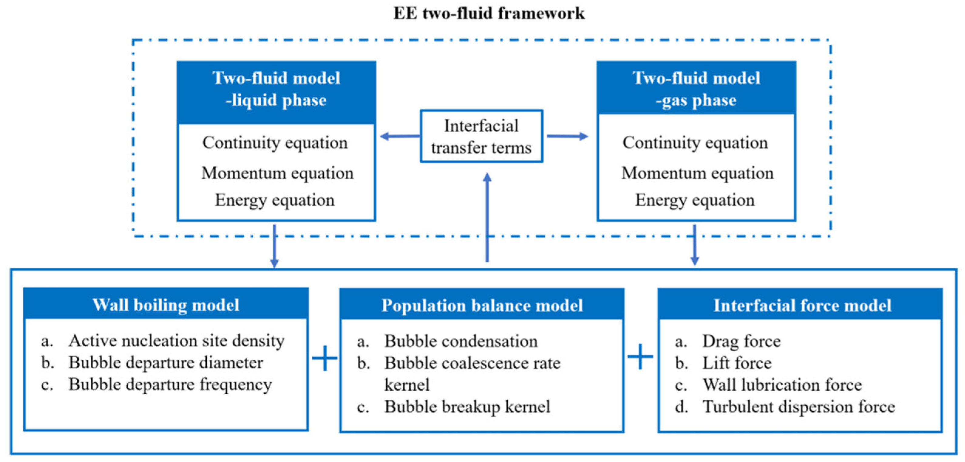
2. Computational Multiphase Flow Dynamics (CMFD) Modelling

Figure 1 illustrates the gas–liquid flow within the Eulerian–Eulerian (EE) two-fluid framework, incorporating the two-fluid model coupled with wall boiling, the Population Balance Model (PBM) and the interfacial force model that both contribute to the two-fluid model and interfacial transfer terms. The details of each model and their respective equations are described in this section, organized into corresponding subsections.

2.1. Governing Equations

The two–fluid model treats each phase as inter-penetrating continua. It solves individual transport equations for the mass, momentum and energy of each phase, while a pressure field is shared for all phases. Eulerian averaging [50,51,52] of the transport equations results in additional interactions between the phases. Models for closure, such as drag, lift forces and interphase heat transfer, are necessary to account for these interactions.

Continuity Equation

The conservation of mass for a generic phase $i$ is given by:

$${\displaystyle \frac{\mathsf{\partial }}{\mathsf{\partial }t}}{\displaystyle \underset{V}{\int }{\alpha }_i{\rho }_{i}dV+{\displaystyle \underset{V}{\oint }{\alpha }_i{\rho }_i{v}_i.da={\displaystyle \underset{V}{\int }{\displaystyle {\sum }_{j\ne i}(m_{ij}-}}}}{m}_{ji})dV+{\displaystyle \underset{V}{\int }{s}_i^{\alpha }dV}$$

(1)

where ${\alpha }_i$ is the volume fraction of phase $i$; ${\rho }_i$ is the density, kg/m³; $v_i$ is the velocity, m/s; $m_{ij}$ is the mass transfer rate to phase $i$ from phase $j$, kg/s; $m_{ji}$ is the mass transfer rate to phase $j$ from phase $i$, kg/s; $s_i^{\alpha }$ is a user-defined phase mass source term.

Momentum Equation

The momentum balance for the generic phase $i$ is given by:

$$\begin{array}{l}{\displaystyle \frac{\mathsf{\partial }}{\mathsf{\partial }t}}{\displaystyle \underset{V}{\int }{\alpha }_i{\rho }_i{v}_{i}dV+{\displaystyle \underset{A}{\oint }{\alpha }_i{\rho }_i{v}_i\otimes v_i.da=-{\displaystyle \underset{V}{\int }{\alpha }_i\nabla pdV}}}\\ +{\displaystyle \underset{V}{\int }{\alpha }_i{\rho }_{i}gdV}+{\displaystyle \underset{A}{\oint }\left[{\alpha }_i({\sigma }_i+{\sigma }_i^t\right]}.da+{\displaystyle \underset{V}{\int }{M}_{i}dV}\\ +{\displaystyle \underset{V}{\int }{(F_{\mathrm{int}})}_{i}dV+}{\displaystyle \underset{V}{\int }{s}_i^{\alpha }dV+}\underset{V}{\int }{\displaystyle \sum _{i=1}^n}{(m_{ij}{v}_j-m_{ji}{v}_i)}^{\mathit{\text{dV}}}\end{array}$$

(2)

where $p$ is the pressure, assumed to be equal in all phases, Pa; $g$ is the gravity vector, m/s²; ${\sigma }_i$ and ${\sigma }_i^t$ are the molecular and turbulent stresses, respectively, N/m²; $M_i$ is the interphase momentum transfer per unit volume, ${(F_{\mathrm{int}})}_i$ represents internal forces, N.

Energy Equation

$$\begin{array}{l}{\displaystyle \frac{\mathsf{\partial }}{\mathsf{\partial }t}}{\displaystyle \underset{V}{\int }{\alpha }_i{\rho }_i{E}_{i}dV+{\displaystyle \underset{A}{\oint }{\alpha }_i{\rho }_i{H}_i{v}_i.da=}}{\displaystyle \underset{A}{\oint }{\alpha }_i{k}_{eff,i}\nabla T_{i}da+{\displaystyle \underset{A}{\oint }{\sigma }_v.v_i.da}}\\ +{\displaystyle \underset{V}{\int }{F}_{i.}{v}_{i}dV}+{\displaystyle \underset{V}{\int }{\displaystyle {\sum }_{j\ne i}{Q}_{ij}dV+}}{\displaystyle \underset{V}{\int }{\displaystyle {\sum }_{(ij)}{Q}_i^{(ij)}dV}}\\ +{\displaystyle \underset{V}{\int }{s}_{u,i}dV+}{\displaystyle \underset{V}{\int }{\displaystyle {\sum }_{j\ne i}(m_{ij}-m_{ji})H_i(T_{(ij)})dV}}\end{array}$$

(3)

where $E_i$ is the total energy, J; $H_i$ is the total enthalpy, J; $T_i$ is the viscous stress tensor, N/m²; $k_{eff,i}$ is the effective thermal conductivity, W/mK; $Q_{ij}$ is the interphase heat transfer rate to phase $i$ from phase $j$, $s_{u,i}$ is the energy source, W/m²·K.

Volume Fraction

The share of the flow domain that is occupied by each phase is given by its volume fraction.

$$V_i={\displaystyle \underset{V}{\int }{\alpha }_{i}dV}$$

(4)

The volume fractions of each Eulerian phase must fulfil the requirement:

$${\displaystyle \sum _{i=1}^n{\alpha }_i=1}$$

(5)

2.2. RPI Wall Boiling Model

The Rensselaer Polytechnic Institute (RPI) wall boiling model proposed by Kurul and Podowski [53] is used to describe the subcooled boiling process at the heated wall surface, which includes a wall heat flux partitioning method.

The model considers three modes of heat transfer from the wall to the fluid (vapor and liquid). The Kurul and Podowski model is formulated as follows:

$$\stackrel{•}{q}\prime {\prime }_w=\stackrel{•}{q}\prime {\prime }_{conv}+\stackrel{•}{q}\prime {\prime }_{evap}+\stackrel{•}{q}\prime {\prime }_{quench}$$

(6)

$\stackrel{•}{q}\prime {\prime }_w$ Wall heat flux, W/m²; $\stackrel{•}{q}\prime {\prime }_{conv}$ Convective heat flux, W/m²; $\stackrel{•}{q}\prime {\prime }_{evap}$ Evaporative heat flux, W/m²; $\stackrel{•}{q}\prime {\prime }_{quench}$ Quenching heat flux, W/m²;

Modified RPI Wall Boiling model

Subcooled boiling models start with the assumption that only the liquid phase is in contact with the wall. When examining the transition to DNB (Departure from Nucleate Boiling), the contribution of vapor becomes significant. Increasing the wall heat flux further leads to liquid access being limited, which causes vapor heat transfer to remove a portion of the wall heat flux and elevate the wall temperature.

The representation of heat fluxes is as follows:

$$\stackrel{•}{q}\prime {\prime }_w=\left(\stackrel{•}{q}\prime {\prime }_{conv}+\stackrel{•}{q}\prime {\prime }_{evap}+\stackrel{•}{q}\prime {\prime }_{quench}\right)\left(1-K_{dry}\right)+K_{dry}\stackrel{•}{q}\prime {\prime }_{dry}$$

(7)

$\stackrel{•}{q}\prime {\prime }_{dry}$ vapor contribution to convective heat flux on single-phase turbulent convection by the vapor, W/m².

$K_{dry}$ wall contact area fraction for the vapor based on either an expression or a transition volume fraction representing the start of wall dry out. Details of all the heat fluxes are summarized in

Table 1. Summary of the contribution of various heat fluxes to the wall heat flux partitioning model.

Heat Fluxes	Forms
$\stackrel{•}{q}\prime {\prime }_{conv}$ Convective Heat Flux (Liquid and gas)	$\stackrel{•}{q}\prime {\prime }_{conv}={\displaystyle \frac{{\rho }_l{c}_{pl}{v}_l^{*}}{t_l^{+}}}\left(T_w-T_l\right)$ $\stackrel{•}{q}\prime {\prime }_{dry}={\displaystyle \frac{{\rho }_g{c}_{pg}{v}_g^{*}}{t_g^{+}}}\left(T_w-T_g\right)$
$\stackrel{•}{q}\prime {\prime }_{evap}$ Evaporative Heat Flux	$\stackrel{•}{q}\prime {\prime }_{evap}=n"f\left({\displaystyle \frac{\pi d_w^3}{6}}\right){\rho }_g{h}_{lg}$
$\stackrel{•}{q}\prime {\prime }_{quench}$ Bubble Induced Quenching Heat Flux	$\stackrel{•}{q}\prime {\prime }_{quench}=h_{quench}\left({\displaystyle \frac{T^{+}(y_{quench})}{T^{+}(y_c)}}\right)(T_{wall}-T_l)$

where $\stackrel{•}{q}\prime {\prime }_{conv}$ Convective heat flux, W/m²; $\stackrel{•}{q}\prime {\prime }_{dry}$ vapor contribution to convective heat flux, W/m²; $\stackrel{•}{q}\prime {\prime }_{evap}$ Evaporative Heat Flux, W/m²; $\stackrel{•}{q}\prime {\prime }_{quench}$ Bubble-Induced Quenching Heat Flux, W/m²; ${\rho }_l$, ${\rho }_g$ are the density of the liquid phase and gas phase, respectively, kg/m³; $v_l^{*}$, $v_g^{*}$, are the velocity of the liquid phase and gas phase, respectively, m/s; $t_l^{+}$, $t_g^{+}$ are the temperature of the liquid cell and gas cell, respectively, K; $c_{pl}$, $c_{pg}$ are the specific heat of the liquid phase and the gas phase, respectively, J/kg·K; $T_w$, $T_l$ and $T_g$ are the temperature of the wall, liquid and gas phases, respectively, K; $n"$ is the nucleation site density, $f$ is the bubble departure frequency, 1/s; $d_w^{ }$ is the bubble departure diameter, m; $h_{lg}$ is the latent heat, J/kg; $h_{quench}$ is the quenching heat transfer coefficient, W/m²K; $T^{+}$ is the dimensionless temperature profile; $y$ is the distance from the wall, m; $c$ is nearest cell center, m.

.

2.3. Closure Models

The two-fluid Eulerian model approach and wall boiling model are commonly utilized and highly adaptable models for simulating multiphase flow boiling. While providing a reasonable level of accuracy, this approach heavily depends on individual phenomenological closure models. The advancement of closure models that offer greater accuracy is a constantly evolving area of research. Current progress is shifting away from correlation-based models and towards physical, mechanistic-based models.

2.3.1. Closure Models for the RPI Wall Boiling Model

The computation of the heat flux components depends on the features of Bubble Departure Diameter, Bubble Departure Frequency and the Nucleation Site Density in the subcooled flow boiling process [33]. The RPI wall boiling model’s accuracy under various operational conditions is determined by three critical parameters: active nucleation site density, bubble departure diameter, and bubble departure frequency, as described below. The complex physics involved in wall boiling makes it infeasible to theoretically determine these parameters. This is due to their dependence not only on operating parameters such as pressure, subcooling, heat flux and liquid flow rate but also on the properties of the surface of the wall [54,55,56].

Active nucleation site density

The density of nucleation sites dictates the number of locations on the heated surface, per unit area, where bubbles form. The density of active nucleation sites is usually influenced by factors such as surface properties, wall superheat and working medium. However, these factors are highly interrelated, making it difficult to distinguish one from the other. In a mechanistic model of subcooled boiling, the nucleation site density is the primary factor that governs the rate of evaporation. This study considers two correlations based on this premise, as outlined in

Table 2. Nucleation site density models’ formulation.

Nucleation Site Density Model	Identifier	Formula
Lemmert Chawla [37,57]	LC	${\displaystyle \frac{n^{″}}{[m^{(-2)}]}}=(m\mathsf{\Delta }{T}_{sup})p$
Hibiki Ishii [38]	HI	$n\prime \prime =\overline{n\prime \prime }\left(1-exp\left[-{\displaystyle \frac{{\theta }^2}{8{\mu }^2}}\right]\right)\left(exp\left[f\left({\rho }^{+}\right){\displaystyle \frac{{\lambda }^{\prime }}{R_c}}\right]-1\right)$

where $n\prime \prime$ is the nucleation site density; $m$ is a calibration constant, with a default value of 185.0/K; $p$ is a superheat exponent, with a default value of 1.805; $\mathsf{\Delta }{T}_{sup}$ is the wall superheat, K; $\overline{n\prime \prime }$ is the average cavity density, with a default value of 4.74 × 10⁵ sites/m⁻²; $\theta$ is the wall contact angle, with a default value of 0.722 radians (41.37°); $\mu$ is the wall contact angle scale, with a standard value of 0.722 radians (41.37°); ${\lambda }^{\prime }$ is the cavity length scale, with default value 2.5 × 10^-6 m; $f\left({\rho }^{+}\right)$ is the logarithmic, non-dimensional density function representing the effect of pressure; $R_c$ is the critical cavity radius.

.

Bubble departure diameter

At the moment when a bubble leaves the nucleation site, its diameter is determined by the bubble departure diameter model. This is the second among the three factors that determine the evaporation rate in subcooled boiling. It relies on different parameters such as the contact angle, mass flow rate, pressure, subcooling and others. This study considers the three most used correlations, depicted in

Table 3. Bubble departure diameter models’ formulation.

Bubble Departure Diameter Model	Identifier	Formula
Tolubinsky Kostanchuk [39]	TK	$d_w=d_{0}exp\left[-{\displaystyle \frac{\mathsf{\Delta }{T}_{sub}}{\mathsf{\Delta }{T}_0}}\right]$
Kocamustafaogullari [40]	KO	$d_w=d_1\theta {\left({\displaystyle \frac{\sigma }{g\mathsf{\Delta }\rho }}\right)}^{0.5}\left({\displaystyle \frac{\mathsf{\Delta }\rho }{{\rho }_g}}\right)$ $d_w={\displaystyle \frac{2.42\times {10}^{-5}{p}^{0.709}a}{\sqrt{b\varphi }}}$
Unal [58]	U	$b={\displaystyle \frac{\mathsf{\Delta }{T}_{sub}}{2(1-{\rho }_g/{\rho }_l)}}$ $\varphi =\left\{\begin{array}{l}{(v_l/v_0)}^{0.47}\hspace{0.17em}{v}_{{ }_l}\ge v_0\\ 1\hspace{0.17em}\hspace{0.17em}\hspace{0.17em}\hspace{0.17em}\hspace{0.17em}\hspace{0.17em}\hspace{0.17em}\hspace{0.17em}\hspace{0.17em}\hspace{0.17em}\hspace{0.17em}{v}_{{ }_l}<v_0\end{array}\right\}$

where $d_w$ is bubble departure diameter, m; $d_0$ is the reference diameter with default value 0.0006 m; $\mathsf{\Delta }{T}_0$ is the reference subcooling with default value 45 K; $\mathsf{\Delta }{T}_{sub}$ is the subcooling of the liquid next to the wall; $d_1$ is a calibration constant, with a default value of, 1.5126 × 10⁻⁵ m/degree; $\theta$ is the wall contact angle, with a default value of 0.722 radians (41.37°); $\sigma$ is the surface tension, N/m; $g$ is the acceleration due to gravity, m/s²; $\mathsf{\Delta }\rho$ is the difference in density between the liquid and gas phase, kg/m³; ${\rho }_l$, ${\rho }_g$ are liquid and vapor phase density, kg/m³; $p$ is the local pressure, Pa; $T_w$ is the wall temperature, K; $T_{sat}$ is the superheat temperature, K; $k_w$ is the thermal conductivity of the wall material, W/m·K; $c_{pw}$ is the specific heat of the wall material, J/g·K; ${\lambda }_{lg}$ is the latent heat, J/kg; $v_l$ is the liquid velocity near the wall, m/s; $v_0$ = 0.61, m/s.

.

Bubble Departure Frequency

The bubble departure frequency determines how many bubbles leave a nucleation site per second. This is the last of three key factors determining the evaporation rate in subcooled boiling. System pressure, heat flux, and liquid flow rate exert an influence on it [59]. However, it is regarded as having the least significant impact on the simulation outcomes. Rather than contrasting sub-models for this parameter, the Cole model [41] opts for the current approach, which stands as the most frequently employed.

The widely used correlation developed by Cole takes the form of:

$$f=\sqrt{{\displaystyle \frac{4}{3}}{\displaystyle \frac{g({\rho }_l-{\rho }_g)}{d_w{\rho }_l}}}$$

(8)

where $f$ is the bubble frequency, 1/s; $g$ is the gravity, m/s²; ${\rho }_l \mathrm{a}\mathrm{n}\mathrm{d} {\rho }_g$ are the density of the liquid and gas, respectively, kg/m³; $d_w$ is the bubble departure diameter, m.

This uses a typical bubble rise velocity (estimated using unit drag coefficient) as the velocity scale, and bubble diameter as the length scale.

Sub-model combination of Bubble Dynamics for wall boiling model

The predictive capability of the wall heat flux partitioning model depends on the combination of the active nucleation site density, bubble departure diameter and bubble departure frequency. Nonetheless, the abundance of sub-models for each bubble parameter presents a significant challenge in identifying an optimal combination that consistently delivers high accuracy across a broad spectrum of flow conditions. The present study addresses this challenge by the evaluation of specific combinations, as detailed in

Table 4. Various combinations of sub-models for nucleation site density ($n\prime \prime$), bubble departure diameter ($d_w$), and bubble frequency ($f$).

No	$\mathit{n}\prime \prime$	${\mathit{d}}_{\mathit{w}}$	$\mathit{f}$	Identifier
1	LC	TK	Cole	LC-TK
2	LC	KO	Cole	LC-KO
3	LC	U	Cole	LC-U
4	HI	TK	Cole	HI-TK
5	HI	KO	Cole	HI-KO
6	HI	U	Cole	HI-U

.

2.3.2. Models for Interfacial Forces

The closure laws of interfacial forces are applied for the interaction between primary and secondary phases in the form inter-phase momentum exchange. To calculate the inter-phase momentum exchange between the liquid and gas phases, the momentum equation is solved for both phases. These interfacial momentum forces are included in the momentum equation as source terms. The distribution of bubbles within the liquid is influenced by these forces, including drag force, lift force, wall lubrication force, virtual mass force and turbulence dispersion force. Thus, the total interfacial forces responsible for momentum exchange are given by the linear combination of individual force [60,61,62].

$$M_i=\sum _{j\ne i}(F_{ij}^D+F_{ij}^L+F_{ij}^{VM}+F_{ij}^{TD}+F_{ij}^{WL})$$

(9)

where $F^D$ is the drag force, N; $F^L$ Lift force, N; $F^{VM}$ virtual mass force, N; $F^{TD}$ turbulent dispersion force, N; $F^{WL}$ wall lubrication force, N.

The accuracy of CFD simulations for bubbly flow is significantly influenced by the selection of closure models for interfacial forces, and the precision of results is constrained by the appropriateness of these chosen closure models. Validating individual models for interfacial forces through isolated effect tests presents a challenge. Therefore, the present study also conducts simulations of interfacial forces and their closure models to ascertain their applicability in refrigerant flow boiling applications.

Drag force (D)

The drag force accounts for the viscous effects that either decelerate or accelerate a particle of the dispersed phase (e.g., gas bubble, liquid droplet, or solid particle) within the fluid by the continuous phase. Typically, the interphase drag force is computed by employing a drag coefficient as a function. The definition of the drag force is given by:

$$F_{ij}{ }^D=A_D{v}_r$$

(10)

where $A_D$ is the linearized drag coefficient and $v_r$ the relative velocity between the phases, m/s².

$$A_D=C_D{\displaystyle \frac{1}{2}}{\rho }_c\left|v_r\right|\left({\displaystyle \frac{a_{cd}}{4}}\right)$$

(11)

The standard drag coefficient $C_D$ is composed of two factors:

$$C_D=f_D{C}_{D\infty }$$

(12)

where $C_{D\infty }$ is the single particle drag coefficient, $f_D$ is a drag correction factor for the shape of non-spherical particles. Schiller [63] established a correlation for various ranges of the bubble Reynolds number ($\mathrm{Re}$), setting the minimum drag coefficient at 0.44 for $\mathrm{Re}$ values upper 1000. Rusche and Issa [64] developed drag coefficient for high volume fraction that spans from one when the dispersed phase volume fraction is zero and increases exponentially. Bozzano–Dente Drag Coefficient [65] covers a broad spectrum of bubbly flow regimes and regimes and accommodates various bubble shapes through a unified expression. This coefficient was formulated specifically for a scenario involving a single bubble ascending in a liquid column under the influence of gravity. The Hamard and Rybczynski drag model [66] is employed for droplets of viscous Newtonian fluid dispersed within another immiscible viscous Newtonian fluid. The Tomiyama correlation [67] is applicable to systems under a wide range of conditions, defined by the Eotvos ($\mathrm{E}\mathrm{o}$), Morton ($\mathrm{M}\mathrm{o}$) and Reynolds ($\mathrm{Re}$) numbers, as indicated in

Table 5. Interfacial drag coefficient models.

Model	Identifier	Equation
Schiller and Naumann [63]	SN	$C_D=\left\{\begin{array}{l}{\displaystyle \frac{24}{{\mathrm{Re}}_d}}(1+0.15{\mathrm{Re}}_d^{0.687})\hspace{0.17em}\hspace{0.17em}\hspace{0.17em}\hspace{0.17em}\hspace{0.17em}{\mathrm{Re}}_d\le 1000\\ 0.44\hspace{0.17em}\hspace{0.17em}\hspace{0.17em}\hspace{0.17em}\hspace{0.17em}\hspace{0.17em}\hspace{0.17em}\hspace{0.17em}\hspace{0.17em}\hspace{0.17em}\hspace{0.17em}\hspace{0.17em}\hspace{0.17em}\hspace{0.17em}\hspace{0.17em}\hspace{0.17em}\hspace{0.17em}\hspace{0.17em}\hspace{0.17em}\hspace{0.17em}\hspace{0.17em}\hspace{0.17em}\hspace{0.17em}\hspace{0.17em}\hspace{0.17em}{\mathrm{Re}}_d>1000\hspace{0.17em}\end{array}\right\}$
Rusche–Issa Drag Coefficient [64,69]	RI	$C_D=\left\{\begin{array}{l}{\displaystyle \frac{24}{{\mathrm{Re}}_{cd}}}(1+0.15{\mathrm{Re}}_b^{0.687})\hspace{0.17em}\hspace{0.17em}\hspace{0.17em}\hspace{0.17em}\hspace{0.17em}\hspace{0.17em}\hspace{0.17em}\hspace{0.17em}\hspace{0.17em}{\mathrm{Re}}_b\le 1000\\ 0.44\hspace{0.17em}\hspace{0.17em}\hspace{0.17em}\hspace{0.17em}\hspace{0.17em}\hspace{0.17em}\hspace{0.17em}\hspace{0.17em}\hspace{0.17em}\hspace{0.17em}\hspace{0.17em}\hspace{0.17em}\hspace{0.17em}\hspace{0.17em}\hspace{0.17em}\hspace{0.17em}\hspace{0.17em}\hspace{0.17em}\hspace{0.17em}\hspace{0.17em}\hspace{0.17em}\hspace{0.17em}\hspace{0.17em}\hspace{0.17em}\hspace{0.17em}\hspace{0.17em}\hspace{0.17em}\hspace{0.17em}\hspace{0.17em}\hspace{0.17em}{\mathrm{Re}}_b>1000\hspace{0.17em}\end{array}\right\}$ $f({\alpha }_d)=e^{k1\alpha d}+{\alpha }_d^{K{2}_{ }}$
Symmetric Drag Coefficient	Sym	$A_{cd}^D={\displaystyle \frac{3}{4}}{C}_D{\displaystyle \frac{{\alpha }_c{\alpha }_d({\alpha }_c{\rho }_c+{\alpha }_d{\rho }_d)}{({\alpha }_c{l}_c+{\alpha }_d{l}_d)}}\left|v_r\right|$ Where $C_D$ as per Schiller and Naumann and ${\mathrm{Re}}_{cd}={\displaystyle \frac{({\alpha }_c{\rho }_c+{\alpha }_d{\rho }_d)({\alpha }_c{l}_c+{\alpha }_d{l}_d)\left|v_r\right|}{({\alpha }_c{\mu }_c+{\alpha }_d{\mu }_d)({\alpha }_c+{\alpha }_d)}}$
Bozzano-Dente Drag Coefficient for Bubbles [65]	BD	$C_D=f{\left({\displaystyle \frac{a}{R_0}}\right)}^2$ Where f friction factor and ${(a/R_0)}^2$ is a deformation factor $f=\left({\displaystyle \frac{48}{\mathrm{Re}}}\right){\displaystyle \frac{1+12\mathrm{M}{\mathrm{o}}^{1/3}}{1+36\mathrm{M}{\mathrm{o}}^{1/3}}}+0.9{\displaystyle \frac{\mathrm{E}{\mathrm{o}}^{3/2}}{1.4(1+30\mathrm{M}{\mathrm{o}}^{1/6})+\mathrm{E}{\mathrm{o}}^{3/2}}}$ ${\left({\displaystyle \frac{a}{R_0}}\right)}^2\cong {\displaystyle \frac{10(1+1.3\mathrm{M}{\mathrm{o}}^{1/6})+3.1\mathrm{E}\mathrm{o}}{10(1+1.3\mathrm{M}{\mathrm{o}}^{1/6})+\mathrm{E}\mathrm{o}}}$
Hamard and Rybczynski Drag Coefficient for Droplets [66]	HR	$C_D={\displaystyle \frac{24}{\mathrm{Re}}}Y$ $where$ $Y={\displaystyle \frac{2+3X_E}{3+3X_E}}$, $X_E={\displaystyle \frac{{\mu }_d}{{\mu }_c}}$
Tomiyama Drag Coefficient for Bubbles [67]	Tom	$Pure\hspace{0.17em}\hspace{0.17em}:$ $C_D=\max \left[\min \left({\displaystyle \frac{16}{\mathrm{Re}}}(1+0.15{\mathrm{Re}}^{0.687}),{\displaystyle \frac{48}{\mathrm{Re}}}\right),{\displaystyle \frac{8\mathrm{E}\mathrm{o}}{3(\mathrm{E}\mathrm{o}+4)}}\right]$ $Moderate \hspace{0.17em}:$ $C_D=\max \left[\min \left({\displaystyle \frac{24}{\mathrm{Re}}}(1+0.15{\mathrm{Re}}^{0.687}),{\displaystyle \frac{72}{\mathrm{Re}}}\right),{\displaystyle \frac{8\mathrm{E}\mathrm{o}}{3(\mathrm{E}\mathrm{o}+4)}}\right]$ $Contaminated:$ $C_D=\max \left[\min \left({\displaystyle \frac{24}{\mathrm{Re}}}(1+0.15{\mathrm{Re}}^{0.687})\right),{\displaystyle \frac{8\mathrm{E}\mathrm{o}}{3(\mathrm{E}\mathrm{o}+4)}}\right]$ $\begin{array}{l}{10}^{-2}<\mathrm{E}\mathrm{o}<{10}^3,\\ \hspace{0.17em}{10}^{-3}<{\mathrm{Re}}_b<{10}^6,\hspace{0.17em}\\ {10}^{-14}<\mathrm{M}\mathrm{o}<{10}^7\end{array}$
Wang Drag Coefficient for Bubbles [68]	Wang	$C_D=e^{\left[a+b\ln {\mathrm{Re}}_d+c{(\ln {\mathrm{Re}}_d)}^2\right]}$ ${\mathrm{Re}}_d\le 1\hspace{0.17em}\hspace{0.17em}:\hspace{0.17em}\hspace{0.17em}a=\ln \hspace{0.17em}24,\hspace{0.17em}b=-1,\hspace{0.17em}\hspace{0.17em}c=0$ $\begin{array}{l}1<{\mathrm{Re}}_d\le 450\hspace{0.17em}:\hspace{0.17em}\hspace{0.17em}a=2.699467,\hspace{0.17em}\\ b=-0.33581596,\hspace{0.17em}\hspace{0.17em}c=-0.07135617\end{array}$ $\begin{array}{l}450<{\mathrm{Re}}_d\le 4000:\\ a=-51.77171,\hspace{0.17em}b=13.1670725,\hspace{0.17em}\hspace{0.17em}c=-0.8235592\end{array}$ $\begin{array}{l}{\mathrm{Re}}_d>4000\hspace{0.17em}:\\ a=\ln (8/3),\hspace{0.17em}b=0,\hspace{0.17em}\hspace{0.17em}c=0\end{array}$

where $C_D$ is drag coefficient; ${\mathrm{Re}}_d$ is dispersed phase Reynolds number; K1 = 3.64 for gas bubble, 2.10 for liquid droplet and 2.68 for solid particles, K2 = 0.864 for gas bubble, 0.249 for liquid droplet and 0.430 for solid particles; $\alpha$ is the interfacial area density for the two-phase interaction, m²; $f$ is drag correction factor; $v_r$ is relative velocity, m/s; d represents dispersed phase; $l_c$ is the interaction length scale, m; $l_d$ is the inverted topology length scale, m; $Mo$ is the Morton number; $Eo$ is the Eotvos number; ${\mu }_c$ is the dynamic viscosity of the continuous phase, N/s·m²; ${\mu }_d$ is the dynamic viscosity of the dispersed phase, N/s·m².

. The drag coefficient for the Tomiyama correlation is evaluated for a single bubble, based on three levels of contamination: pure, moderately contaminated and contaminated systems. In an air–water system, tap water represents the contaminated system, water that has been distilled two or more times represents the pure system, and water with an intermediate level of purity represents the moderately contaminated system. Wang [68] proposed a drag coefficient for concentrations of air bubbles in water at near atmospheric pressure. All investigated drag coefficient models in the present study are summarized in Table 5.

Drag Corrections

Drag correction is defined as the alterations in the single-particle drag coefficient model due to concentration in a multi-particle system. In this study, the Volume Fraction Exponent Drag Correction was implemented due to its coverage of several regimes of practical applications, including small and large spherical particles.

$$f_D={\alpha }_c^{nD}$$

(13)

where nD is some constant power.

Lift force (L)

In non-uniform continuous-phase flow, a lift force applies on the bubble, acting perpendicular to the rotation and relative velocity vector. This force is derived by Auton et al. [70] as:

$$F_{ij}^L=C_{L,effective}{\alpha }_d{\rho }_c[v_r\times (\nabla \times v_c)]$$

(14)

where $C_{L,effective}$ calculated from the Lift Coefficient ($C_L$) and the Lift Correction (f_l).

The Tomiyama lift coefficient [71] was established by using experimental trajectories of individual bubbles in a high-viscosity system and found similar values for a small bubble in a low-viscosity, air–water system. The Sugrue lift coefficient [72] considered drift phenomena, bubble interaction probability and the maximum packing factor for dispersed bubbly flow. Both lift coefficient formulas examined for this study are listed in

Table 6. Lift force coefficient models.

Model	Identifier	Formula
Tomiyama Lift Coefficient [71]	Tom	$C_L=\left\{\begin{array}{l}\min [0.288\tanh (0.121\mathrm{Re}),f_T\\ f_T\\ -0.27\end{array}\right.$   $\begin{array}{l}\mathrm{E}{\mathrm{o}}_d<4\\ 4\le \mathrm{E}{\mathrm{o}}_d\le 10\\ 10<\mathrm{E}{\mathrm{o}}_d\end{array}$ $f_T=0.00105\mathrm{E}{\mathrm{o}}_d^3-0.0159\mathrm{E}{\mathrm{o}}_d^2+0.474$ $\mathrm{E}{\mathrm{o}}_d=E\mathrm{o}\times {\mathrm{E}}^{-2/3}$ $\mathrm{E}={\displaystyle \frac{1}{1+0.163\mathrm{E}{\mathrm{o}}^{0.757}}}$
Sugrue Lift Coefficient [72]	Su	$C_L=f({\mathrm{W}}_{\mathrm{o}})f(\alpha )$ $f({\mathrm{W}}_{\mathrm{o}})=\min [0.03,5.0404-{\mathrm{W}}_{\mathrm{o}}^{0.0108}]$ $f(\alpha )=\min [1.0155-0.015e^{8.0506\alpha }]$

where $C_L$ is the lift coefficient; $\mathrm{Re}$ is the Reynolds number; $\mathrm{E}{\mathrm{o}}_d$ is the modified Eotvos number that is based on the maximum horizontal dimension of a bubble; $W_o$ is the Wobble number.

.

Lift Correction

A robust correlation between the lift correction and drag correction was identified. Given the limited literature on lift correction, an approximation of a perfect correlation between lift correction and drag correction is considered. The available choices are as follows:

Drag Correlated (DC)

This approach employs the Drag Coefficient Correction as an estimate for the Lift Coefficient Correction, proving particularly beneficial when modeling swarming scenarios.

Podowski Near Wall Adjustment (Pwall)

The near-wall adjustment by Podowski [73] is a simplified correction that disregards wall lubrication.

The lift coefficient is C_L adjusted as:

$$C_L=\left\{\begin{array}{l}0\\ C_{L0}(3{({\displaystyle \frac{2y}{D_b}}-1)}^2-2{({\displaystyle \frac{2y}{D_b}}-1)}^3)\\ C_{L0}\end{array}\right. \begin{array}{l}{\displaystyle \frac{y}{D_b}}<0.5\\ 0.5\le {\displaystyle \frac{y}{D_b}}\le 1.0\\ 1.0<{\displaystyle \frac{y}{D_b}}\end{array}$$

(15)

Turbulent Dispersion

The turbulent dispersion force is a hydrodynamic force arising from the interaction between turbulent eddies in the continuous phase and the dispersed phase. It holds a pivotal role in shaping the radial distribution of the bubble volume fraction profile [74]. The term is expressed in the following manner:

$$F_{ij}{ }^{TD}=A_D{v}_{TD}$$

(16)

$$D_{TD}=C_0{\displaystyle \frac{v_c^t}{{\sigma }_{\alpha }}}I$$

(17)

$F_{ij}^{TD}$ is the force per volume applied to the continuous phase momentum equation due to the dispersed phase, N. $v_{TD}$ is a relative drift velocity, m/s; $D_{TD}$ is the tensor diffusivity coefficient. $v_c^t$ is the continuous phase turbulent kinematic viscosity, m²/s; ${\sigma }_{\alpha }$ is the turbulent Prandtl number for volume fraction. $C_0$ is the constant to test the sensitivity of the solution to this term as an empirical parameter in the range of 0.1–1.0. I is the identity matrix. The sensitivity of this empirical parameter was examined in the context of refrigerant flow boiling.

Virtual Mass Force

The virtual mass force arises from the energy transfer between an accelerating bubble and the surrounding liquid, where the liquid attempts to acquire the kinetic energy of the bubble. The presence of the virtual mass term can affect the path of bubbles in a steady swirling flow. The inclusion of the virtual mass term in non-accelerating flows can reduce their sensitivity to momentum or pressure relaxation factors by narrowing the range of response timescales across different phases [75].

Auton et al. [68] proposed a two-phase formulation for the virtual mass force as formulated below:

$$F_{ij}{ }^{VM}=C_{VM}{\rho }_c{\alpha }_d(a_j-a_i)$$

(18)

where $C_{VM}$ is the virtual mass coefficient. c is the continuous phase, $a_i \mathrm{a}\mathrm{n}\mathrm{d} a_j$ are the acceleration of phases i and j, m/s². According to inviscid flow theory [76], the virtual mass coefficient for a spherical particle accelerating in an unbounded three-dimensional fluid is 0.5. Zuber [77] employed this formulation to approximate the virtual mass coefficient for an infinite array of particles. It is well-suited for enhancing accuracy in modeling the impact of increasing particle concentration or multiple dispersed phases in accelerating flows. Both formulations are presented in

Table 7. Virtual mass coefficient models.

Model	Formula
Spherical Particle Virtual Mass Coefficient [76]	$C_{VM,sphere}=0.5$ $C_{VM}={\left[{\left(C_{VM,sphere}\right)}^{-2}+C_{VM,\max }{({\alpha }_{c,}{\gamma }_{\min })}^{-2}\right]}^{-1/2}$
Zuber Virtual Mass Coefficient [77]	$C_{VM,Zuber}=0.5{\displaystyle \frac{1+2{\alpha }_d}{1-{\alpha }_d}}$

where $C_{VM}$ is the virtual mass coefficient; ${\alpha }_d$ is the sum of dispersed phase volume fractions; ${\gamma }_{\min }$ is the free stream fraction, value −10.

.

From the literature review, it is apparent that the virtual mass force plays a crucial role in accelerated flow. However, in the majority of bubbly flow simulations, this force is either disregarded or assigned a constant value. While using a constant value may produce satisfactory CFD simulation results, it may not accurately represent the true characteristics of multiphase flow, such as the impact of walls on gas volume fraction [19]. In the present study, a constant value for the virtual mass coefficient and various models mentioned above are simulated to analyze the selectivity of this parameter.

Wall Lubrication

This is another significant force that affects a bubbly flow regime, besides drag force. When bubbles are close to the wall, they tend to concentrate without attaching to it. Hence, the concentration of bubbles near the wall reduces, resulting in a local decrease in the bubble volume fraction. This phenomenon leads to the emergence of a lubrication force caused by surface tension, which pushes the bubbles away from the wall and prevents secondary phase particles from attaching to it [32]. To accurately predict the reduction of gas volume fraction near the wall in Computational Multiphase Fluid Dynamics (CMFD), relying solely on lift, drag, and turbulent dispersion forces may not be sufficient. Among the different available models, Antal et al. [78] wall lubrication models are widely adopted by most researchers. Hence, for the present study, the Antal model was implemented to conduct the simulation, as formulated below:

$$F_{ij}^{WL}=-C_{WL}(y_w){\alpha }_d{\rho }_c{\displaystyle \frac{{\left|v_{r,\parallel }\right|}^2}{d_p}}n$$

(19)

where ${\alpha }_d$ is the bubble volume fraction; $d_p$ is the diameter of the bubble, m; $C_{WL}$ is a function of inverse length. Its value decreases rapidly with increasing distance, $n$ is the outward facing unit normal at the nearest point on the wall, $v_r$ is relative velocity, m/s.

$$v_{r,\parallel }=v_r-(v_r.n)n$$

(20)

The crucial role of interfacial forces in multiphase CFD simulations was observed. However, there is currently no universally accepted method in the open literature for selecting suitable interfacial force models. Further efforts and comprehensive studies are conducted to assess the accuracy and sensitivity of the momentum closure model, aiming to enable its widespread application in computational multiphase flow dynamics (CMFD) simulations of refrigerant flow boiling.

2.3.3. Population Balance Model

A thorough investigation into the bubble size distribution is essential, given its significant impact on the inter-phase heat and mass transfer terms. To incorporate a size distribution of the dispersed phase, it is necessary to integrate the mass and momentum transport equations with a population balance equation (PBE). The two widely utilized numerical approaches for solving the Population Balance Equation (PBE) are the method of moments and the method of classes. The method of the moments-based S-Gamma model [79,80] assumes that the distribution can be expressed by a limited number of parameters. The S-Gamma equations are provided by the following expressions:

$$S_{\gamma }=n{M}_{\gamma }=n{\displaystyle \underset{0}{\overset{\infty }{\int }}{d}^{\gamma }}P(D_d)d{D}_d$$

(21)

$$P\left(D_d\right)={\displaystyle \frac{1}{D_d\sigma \sqrt{2\pi }}}\mathit{exp}\left({\displaystyle \frac{\left(\mathit{ln}(D_d\right)-\mu {)}^2}{2{\sigma }^2}}\right)$$

(22)

$P\left(D_d\right)$ is a log normal distribution of particle sizes $D_d$ represented by the mean particle diameter, m; $\mu$ and its variance, ${\sigma }^2$. $M_{\gamma }$ is the moment size of $P\left(D_d\right)$ and $\gamma$ is the moment number. Several moments conveying information about the bubble population are derived from this distribution. The zeroth moment corresponds to the bubble number density in each cell, the second moment is related to the interfacial area, and the third moment corresponds to the void fraction. Each moment is addressed with individual transport equations. The transport equation for the zeroth moment is as follows:

$${\displaystyle \frac{\mathsf{\partial }{S}_0}{{\mathsf{\partial }}_t}}+\nabla .(S_0{u}_d)=S_{br}+S_{cl}+S_{wb}$$

(23)

This equation includes source terms, $s_{br}$, $s_{cl}$, $s_{wb},$ respectively, corresponding to break up, coalescence and wall boiling, respectively. The zeroth and second moments are computed to yield information on the size distribution. By utilizing this information along with the void fraction, additional details regarding the bubble distribution can be determined.

$$d_{32}={\displaystyle \frac{6{\alpha }_g}{\pi S_2}}={\displaystyle \frac{S_3}{S_2}}$$

(24)

The Adaptive Multiple Size-Group (AMUSIG) [81] model forecasts the size distribution of droplets or bubbles in a dispersed flow regime within a multiphase flow. The continuity and momentum conservation equations of the dispersed phase are enhanced by an additional Population Balance Equation (PBE) for the number density of the population n_i:

$${\displaystyle \frac{\mathsf{\partial }{\overline{n}}_i}{\mathsf{\partial }t}}+\nabla .{\overline{n}}_i\left[{〈u_i〉}_i+D_T\nabla \left(\ln {\overline{\alpha }}_i-\ln {\overline{n}}_i\right)\right]=〈S_i〉$$

(25)

The source term S_i, incorporated on the right side of the number density balance, accounts for the growth or decline of the bubble population due to break up and coalescence effects, respectively. The kernel employed for the break up of bubbles is formulated using an empirical model [82].

$$g_B\left(d_i\right)=h\left(d_i\right)·C_B{\displaystyle \frac{({\epsilon }_c{d}_i{)}^{1/3}}{d_i}}{e}^{-W{e}_{cr.}/We}$$

(26)

where $C_B$ is an empirical constant, ε is the turbulent dissipation, m²/s³, $d_i$ is the bubble diameter, m, and $W{e}_{cr}$ denotes the critical Weber number.

Similarly, the process of bubble coalescence is modeled using an empirical model that assumes various physical processes during the mutual interaction of bubbles [83]. The present study conducts a comprehensive parametric analysis, as outlined in

Table 8. Combination of population balance models along with break up and coalescence models.

No	Model	Break Up Model (BK)	Coalescence Model (CL)
1	S-Gamma	-	-
2	S-Gamma	Power law	-
3	S-Gamma	-	Luo Coalescence Efficiency
4	S-Gamma	Power law	Luo Coalescence Efficiency
5	A-MuSiG	-	-
6	A-MuSiG	Power law	-
7	A-MuSiG	-	Luo Coalescence Efficiency
8	A-MuSiG	Power law	Luo Coalescence Efficiency

, to investigate the population balance approach. By simulating both break-up and coalescence effects, it uniquely explores the intricate dynamics and interactions within the system, offering novel insights into these complex phenomena.

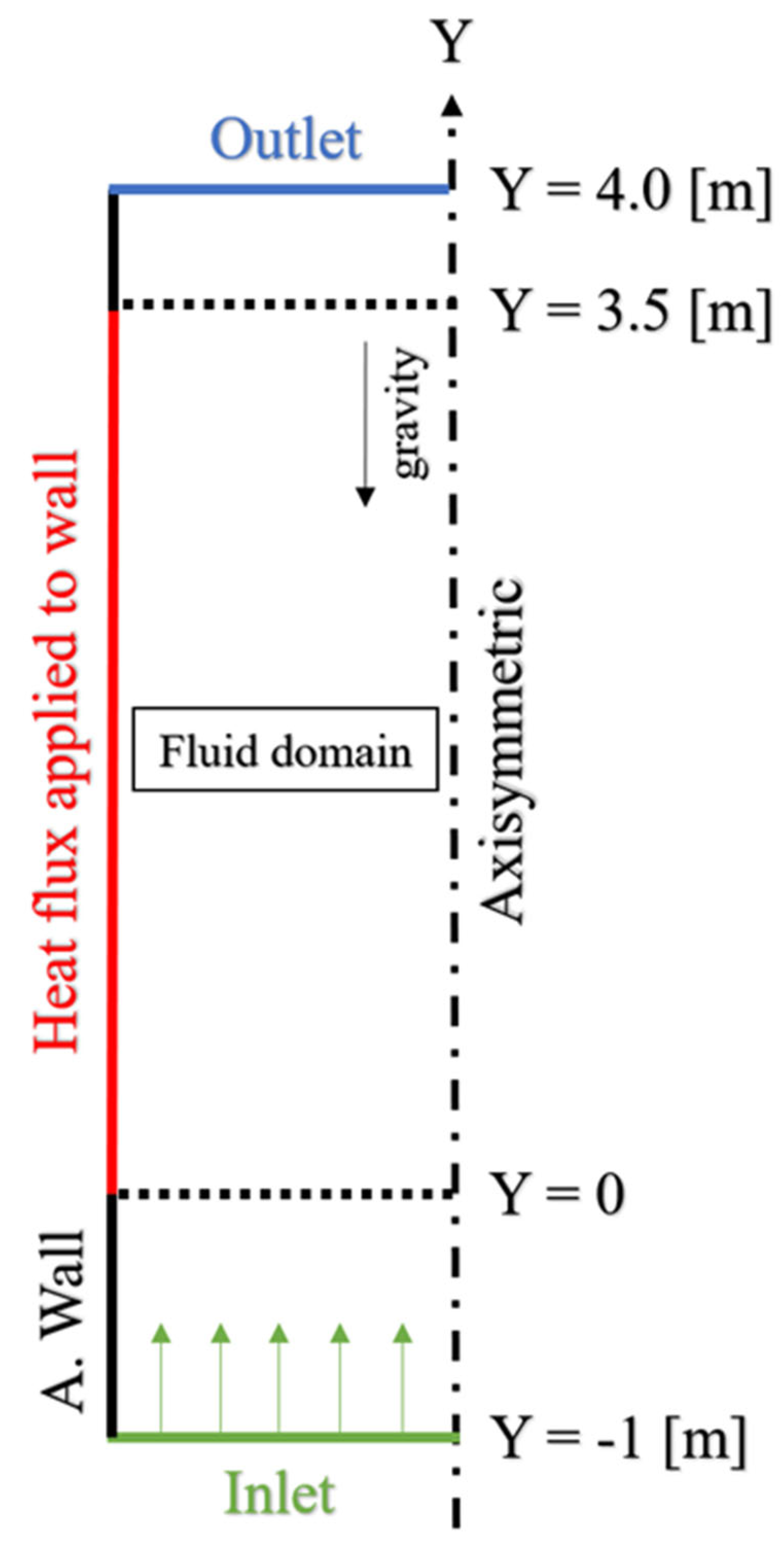
3. Benchmark Data and Simulation Setup

In order to investigate the separate effect of the closure model, the previously published DEBORA experiments [49] are simulated. The flow DEBORA experiments were conducted in a vertical heated pipe with an inner diameter of 19.2 mm, an outer diameter of 21.2 mm and a heated length of 3.5 m, while Freon R12 refrigerant was used as the working fluid. Thermocouples were employed to measure the axial wall temperature profile along the tube. An optical probe was used to measure the radial profiles of the gas volume fraction and the radial liquid temperature profiles at a specific elevation of 3.485 m from the bottom of the heated section. Upstream the heated section, an unheated inlet flow conditioning section of 1 m length was set. Downstream the heated section, an outlet section measuring 0.5 m in length is found. This outlet section was designed to prevent any interference with the flow at the outlet.

Table 9. The selected DEBORA experimental cases for comparison with simulation [82].

Case	p [MPa]	G [kg m−2 s−1]	${\mathit{q}}_{\mathit{n}}^{\mathit{w}}$ [kW m−2]	Tin [°C]	$\mathbf{\Delta }$Tsub[°C]
DEB1	2.62	1996	73.89	68.52	17.91
DEB3	1.46	2028	76.2	28.52	29.58
DEB7	1.46	2024	76.26	44.21	13.89

shows the parameters of the DEBORA experiments selected for the present work. DEB1, DEB3, and DEB7 [49] cases covering three different pressures and high and low inlet liquid subcooling are employed for the validation of the chosen optimal closure models. The material properties and saturation temperature of Freon R12 were taken from the National Institute of Standards and Technology (NIST).

Computational Domain and Boundary Conditions

The DEBORA test cases listed in Table 9 were simulated in M-CFD using Simcenter STAR-CCM+ software version 18.02.010-R8 (2023), incorporating specified built-in sub-closure models within the Eulerian–Eulerian two-fluid framework. To minimize computational effort, all cases are computed over a 2D axisymmetric domain for flow boiling simulation [84,85]. Previous authors have reported only slight differences between the results of two-dimensional and three-dimensional simulations of multiphase flows in cylindrical-shaped tubes [44,86]. In this 2D axisymmetric simulation, a structured directed meshing technique was used to create high-quality swept meshes. This approach involves sweeping a mesh from the geometry’s surfaces through its volume toward a designated target surface. Directed meshing is particularly well-suited for finite volume (FV) fluid flow simulations, as it ensures a structured mesh along the axial direction [87]. The computational domain consists of the fluid region, with the y-axis aligned to the flow direction, cf. Figure 2. The y-axis at X = 0 was set to the axisymmetric boundary condition. The whole dimensions of the fluid domain are 5 m in the axial (y) direction and 9.6 mm in the radial direction. Upstream of the heated section, a fluid domain of 1 m length was introduced as the inlet zone where turbulent flow develops. A uniform velocity was applied at this velocity inlet. A fluid domain of 0.5 m in length was set downstream to mitigate the influence of the outlet boundary condition. At this pressure outlet boundary condition, a constant pressure was set, while assuming saturation conditions for backflow. A uniform heat flux was prescribed on the heated tube wall, and the temperature field at the adiabatic wall was set to a Neumann boundary condition. The physical properties of R12 were fitted as polynomial functions of temperature at a given pressure. A multiphase segregated flow solver was used to perform steady-state iterations until convergence was achieved. Simulations were run until the maximum void fraction in the computational domain converged within 0.1%, ensuring a negligible iteration error, which has proven to be a conservative limit.

For the grid independence test, nine different grid configurations were examined for the different operating conditions of DEB1, DEB3 and DEB7, see

Table 10. Details of grid size for radial division.

Types of Grids
Label	G1 10 × 100	G2 20 × 200	G3 30 × 300	G4 40 × 400	G5 50 × 500
Radial division	10	20	30	40	50
Radial cell size	1.92 mm	0.96 mm	0.64 mm	0.48 mm	0.384 mm
Axial division	100	200	300	400	500
Axial cell Size	50 mm	25 mm	16.67 mm	12.5 mm	10 mm

where Radial division refers to a mesh discretization in the radial direction and Axial division refers to a mesh discretization in the axis direction of a 2D axisymmetric domain.

and

Table 11. Details of grid size for axial division.

Types of Grids
Label	V1 30 × 100	V2 30 × 300	V3 30 × 600	V4 30 × 900
Radial division	30	30	30	30
Axial division	300	400	500	600
Axial cell Size	16.67 mm	12.5 mm	10 mm	8.33 mm

. To investigate the effect of grid resolution, a grid with 10, 20, 30, 40 and 50 cells in lateral and 300, 400, 500, 600, 700 and 800 ones in axial directions were, respectively, tested.

4. Results and Discussion

In the present study, a comprehensive comparison is conducted between the present computational results and a previously published experimental dataset. Particular attention is paid to the axial distribution of wall temperature along the tube, the radial profiles of void fraction and the liquid temperature. The radial profiles for void fraction and liquid temperature are measured at a specific elevation of 3.485 m from the bottom of the heated section in both the computational domain and experimental investigation.

4.1. Grid Dependency Analysis

As one of the initial tasks, a grid dependence test was performed to ensure that the solution obtained from the simulation does not depend on the grid resolution. It involves running the simulation with different grid resolutions and observing how the results vary. The grid dependence check identifies the mesh that enables a solution accuracy of the grid with the least computational cost. A complete check of grid independence is made with axial and radial grid division (with grid details present in Table 10 and Table 11) for all the grids and the three DEORA cases. For convenience, we present only certain results to support the main conclusions drawn hereafter. The alteration in axial mesh distribution was noted to have no impact on the solution (Figure 3a); however, radial distribution with a uniform grid has a noticeable impact on the results. The radial profile of the void fraction is clearly impacted (Figure 3b) with important variations near the wall that modify the radial temperature profile and little variations on the axial profile (Figure 3c,d).

The impact of grid size on temperature and void fraction is primarily attributed to the mass transfer rate. The mass transfer rate is intricately linked to cell liquid temperature, and a finer grid with precise temperature profiles proves advantageous for accurately predicting the mass transfer rate. This rate, coupled with temperature profiles, influences the volume fraction, and variations in mass transfer rates can significantly impact temperature and void fraction, especially in the vicinity of near-wall cell sizes, for example, a faster mass transfer rate accelerates the onset of pseudo-dry out. Given these insights and results from Figure 3, we proceeded to model the test section using uniform grids comprising 30 (radial) × 300 (axial) cells for further simulation cases, aiming to derive optimal predictions for temperature and void fraction. The selection of this grid configuration was based on its accurate correspondence with experimental results.

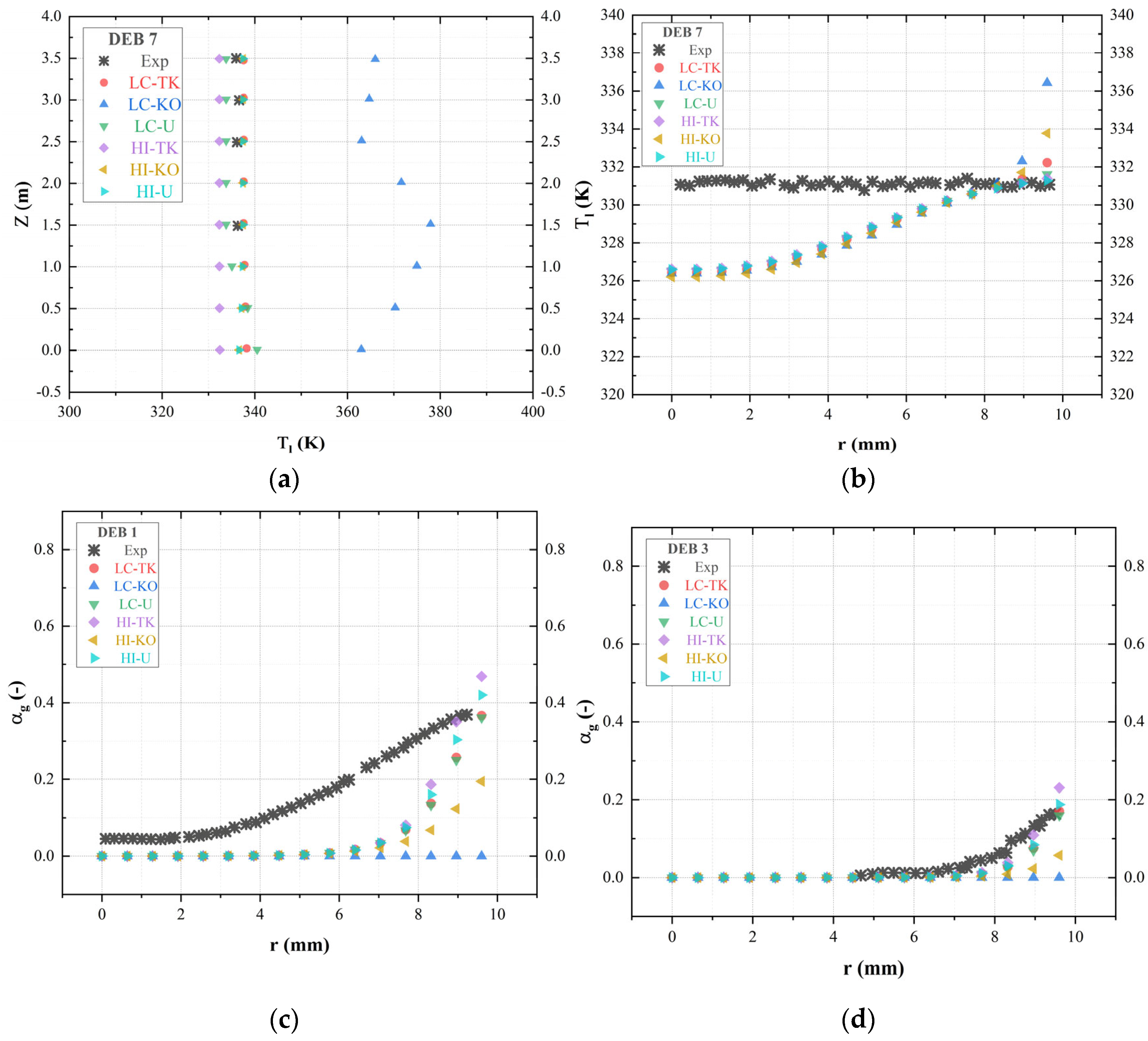
4.2. Boiling Closure

To explore the influence of bubble departure diameter, nucleation site density, and bubble departure frequency parameters, the sub-models detailed in Table 2 and Table 3 were compared with experimental data from DEB1, DEB3, and DEB7 cases. Comparisons include axial distribution of wall temperature, radial profiles of void fraction and of liquid temperature, see Figure 4. For convenience, Figure 4 presents only certain results to illustrate the following assertions.

Notably, the results show that the combination of the Lemmert–Chawla nucleation site density correlation model and the Kocamustafaogullari–Ishii model for bubble departure diameter yield the least accurate results compared to other models. Despite lacking a physical basis, the Lemmert–Chawla correlation and the Tolubinsky–Kostanchuk model for bubble departure diameter demonstrated better accuracy, as these correlations consider the temperature difference between the wall and the bulk liquid. The Kocamustafaogullari Bubble Departure Diameter model, used with the Hibiki–Ishii Nucleation Site Number Density model, provided poor estimates for temperature and void fraction. Although, the combination of Lemmert–Chawla and Unal models overpredicted axial wall temperature but exhibited overall considerable accuracy for void fraction near the wall. The combination of the Hibiki–Ishii Nucleation Site Number Density model and Tolubinsky–Kostanchuk model for bubble departure diameter slightly underpredicted axial wall temperature and overpredicted void fraction. Finally, it was found from Figure 4 that using the combination of the Hibiki–Ishii model for nucleation site density and the Unal model for bubble departure diameter provides the most accurate results. This may be explained by the fact that the Unal model proposes a semi-mechanistic bubble departure diameter model influenced by pressure, wall material, wall sub-heating, and local liquid subcooling, making it suitable for both low and high-pressure conditions.

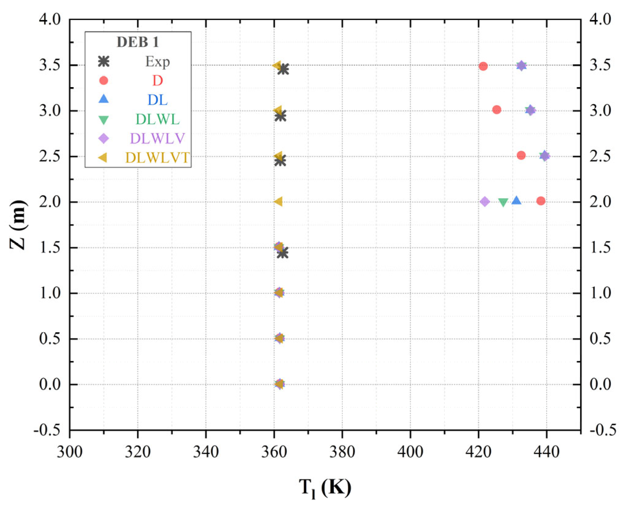
4.3. Momentum Closure

This study investigates the importance of individual interfacial forces and their respective closure models, with initial emphasis on evaluating the impact of each interfacial force on the obtained results. Figure 5 shows the comparison of the axial distribution of wall temperature along the tube with the experimental dataset of DEBORA with the use of the different combinations of closure models of interfacial forces. For convenience, only the DEBORA test 1 is presented (as the conclusion of the comparisons is the same for the three cases). It is clear that interfacial forces models have a positive influence on the result.

Figure 6 presents a comparison of the computed radial liquid temperature with the experimental under various combinations of interphase forces. For convenience only, DEBORA test 7 is presented (as the conclusion of the comparisons is the same for the three DEBORA cases). The Figure shows again clearly that the use of the combination of the different interphase forces models enhances the accuracy of the physics tending to a flatter radial temperature profile as observed in the experimental investigation.

For the void fraction, Figure 7 shows the radial void fraction variation. It is clear again that the use of the combination of the different models enhances the comparison with the DEBORA dataset. For convenience, only DEBORA test 3 is presented.

As a conclusion for momentum closure, the results demonstrate that including different interfacial forces in the whole model set-up positively influences the accuracy of these outcomes, indicating a strong dependency. The exclusion of certain interfacial forces can detrimentally affect result accuracy. The findings reveal indeed that turbulent dispersion force notably influences accuracy, aligning well with the experimental data. Thus, it is recommended to incorporate all five interfacial forces that jointly capture the comprehensive physics of bubbly flow to achieve optimal accuracy.

4.3.1. Sensitivity to Drag Coefficient Model

This study conducts a comparative analysis of seven drag coefficient models, as outlined in Table 5. To assess the influence of different drag force coefficient models, alternative models for other forces are initially examined based on a comprehensive study of general interfacial forces and are kept constant throughout the simulation. Across all three case studies, it is observed that these sub-models have a limited impact on temperature but exhibit noticeable effects on void fraction. For instance, the simulation results for DEB1 are illustrated in Figure 8 and highlight the influence of drag force sub-models on void fraction, which can be significant based on the chosen sub-model. With the exception of the symmetric and Rusche–Issa drag coefficient models, the remaining drag coefficient models demonstrate commendable accuracy in predicting void fraction.

4.3.2. Sensitivity to Lift Force

Within this study, simulations were undertaken to examine the impact of lift force coefficient and lift correction models, as specified in Table 6. Analysis of the simulation results revealed that these sub-models have negligible effects across all three cases, as illustrated in Figure 9. For example, reference data for radial void fraction distribution, (where the differences, even minor, are most important) in the DEB1 case are provided to illustrate this observation. Following the analysis, the Tomiyama lift coefficient model, widely employed in research, and the Podowski Near Wall Adjustment lift correction model were selected for further exploration in subsequent simulations.

4.3.3. Sensitivity to Turbulent Dispersion Force

Extensive investigation into momentum closure mechanisms has unveiled the pivotal role of the turbulence dispersion force in ensuring the accuracy of computational results. Consequently, a sensitivity analysis was conducted to examine the impact of the turbulence dispersion force constant. This study explored three distinct values for the constant, namely 0.1, 0.5, and 1.0, to comprehensively assess its sensitivity across three cases. Analysis of the results depicted in Figure 10, reveals that the turbulence dispersion force constant significantly influences radial void fraction profile, with a noticeable effect on radial liquid temperature. This observation underscores the pivotal role of this force in achieving high accuracy in terms of both void fraction and temperature. Notably, a constant value of 1.0 demonstrates the best accuracy in terms of void fraction and temperature across all three cases. Further investigation into the underlying mechanisms governing the behavior of the turbulence dispersion force may provide valuable insights into its role in multiphase flow simulations.

4.3.4. Sensitivity to Virtual Mass Force

In order to explore the sensitivity of the virtual mass force, different constant values of the virtual mass coefficient and two additional models to derive this constant are investigated, as delineated in Table 7. Specifically, the considered values for the virtual mass coefficient are 0.5 and 0.1. Historically, the constant value of 0.5 has been widely employed in previously published papers dealing with CFD investigations across diverse flow scenarios. Analysis of the present results, reveals minimal influence of this force on both temperature and void fraction for all the three DEBORA cases compared. For convenience Figure 11 illustrate this statement, with the radial temperature profile for DEBORA case 7.

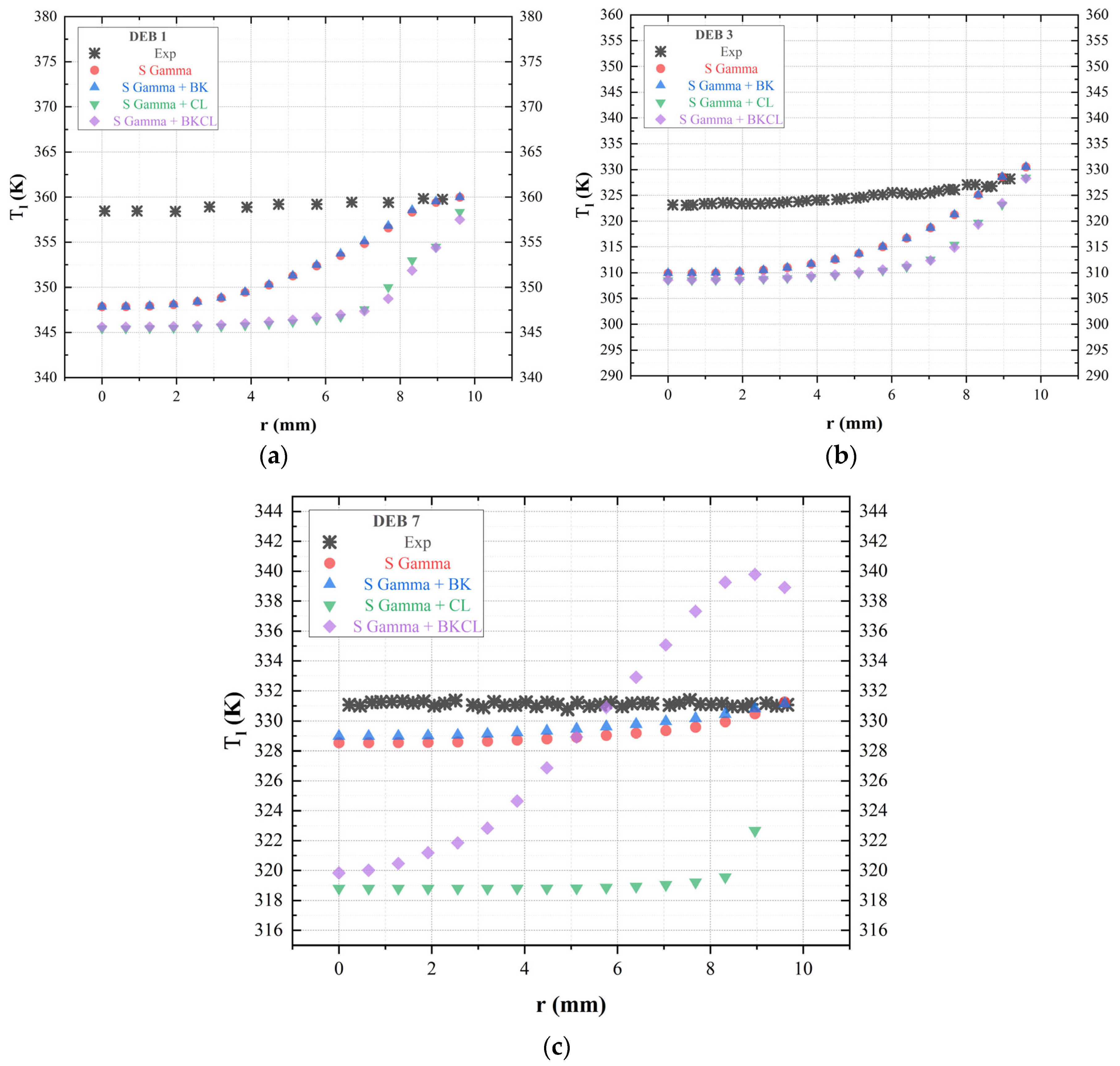
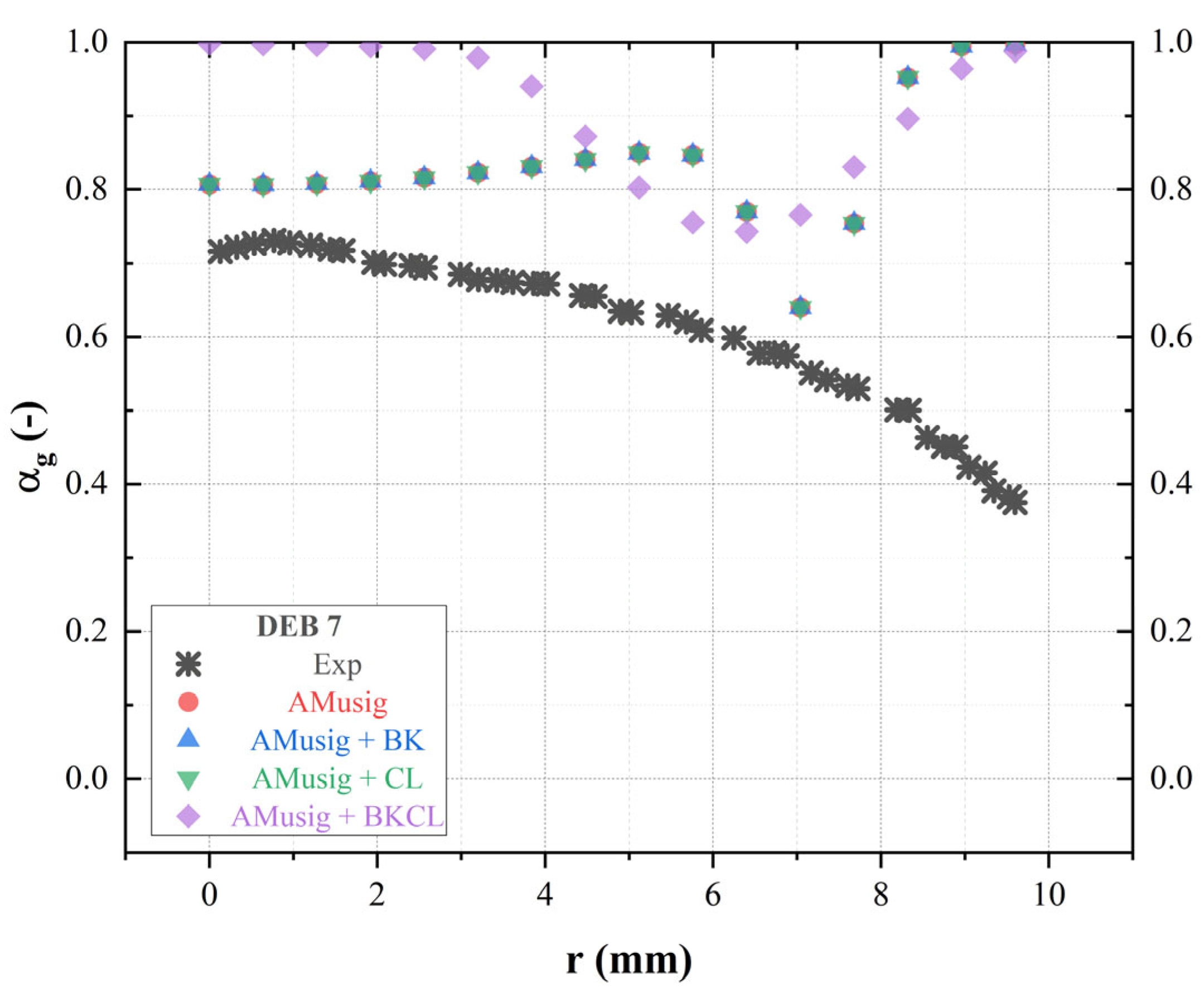
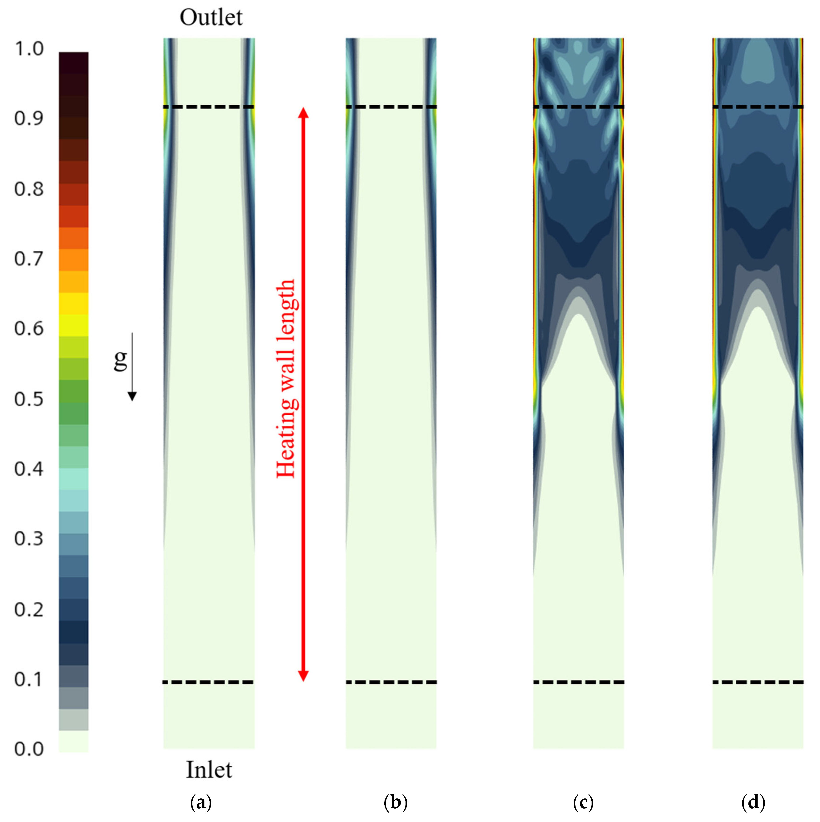
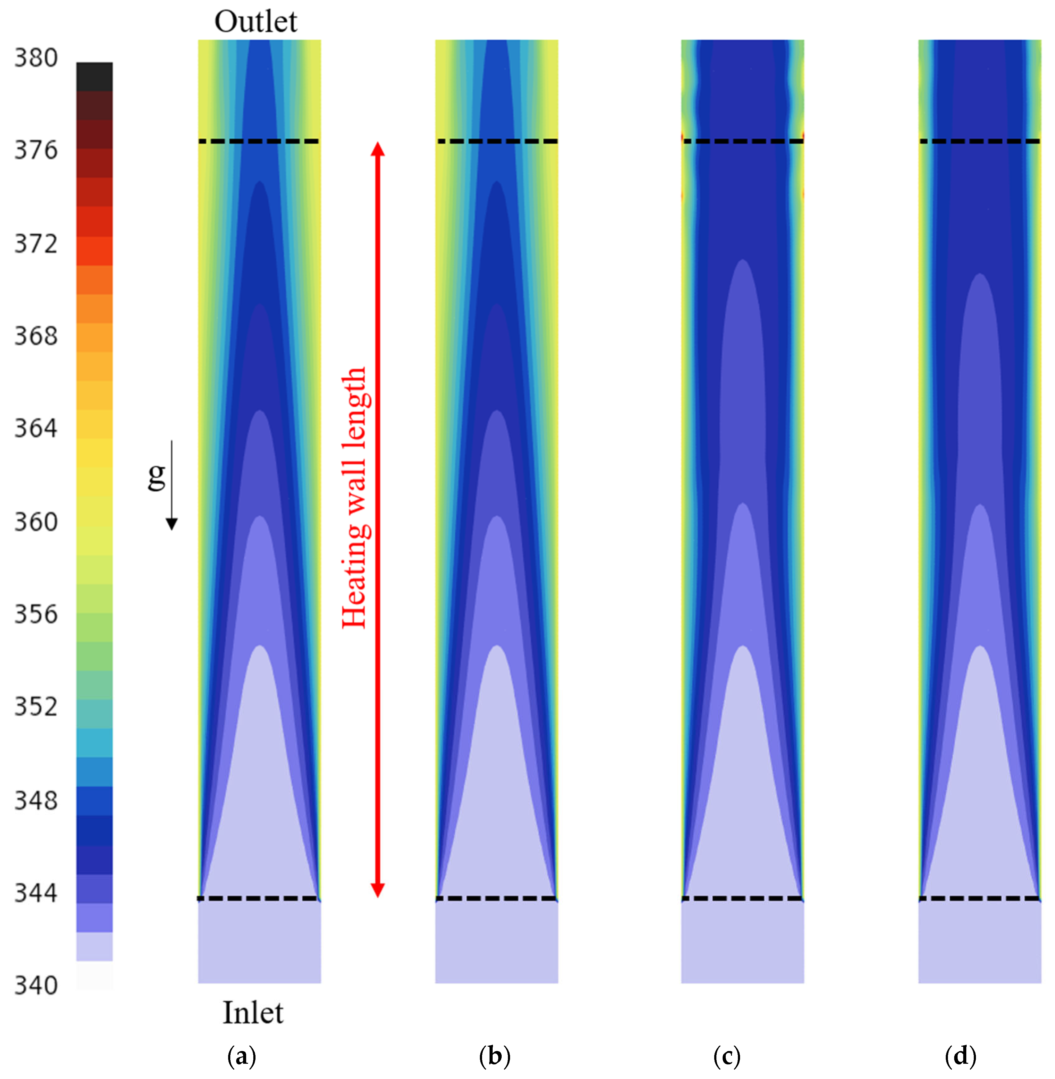
4.4. Sensitivity for Population Balance Approach

This section elucidates and discusses the simulation outcomes utilizing population balance models and their comparison with experimental data. The recent introduction of the population balance approach was an important advance in CMFD. Till now, these models have not been tested thoroughly in the bibliography, and their accuracy when compared with experimental data is still an important issue. In our study, firstly, the simulation results employing the S-Gamma population balance model, incorporating the influences of break up and coalescence, are analyzed below for all the DEBORA cases. Analysis reveals negligible changes in temperature within the near-wall region but a significant influence on temperature in regions farther from the wall. This is illustrated in Figure 12 where the major impact of the population balance model is highlighted within the central region of the flow. Even if the result does not totally match the experimental result, it is clear that this model shows an ability to better simulate the reality of mixing at the heart of the flow. Especially for the case of DEBORA 7 (see Table 9) where the subcooled value is lower and pressure is lower (resulting in higher bubbles growth potential), the break up and coalescence models highly modify the temperature profile of the flow mixture.

Conversely, results for the void fraction profile exhibit a pronounced impact. For example, in Figure 13, one can see the void fraction for the DEBORA case 7. It is clear that the temperature profile is directly linked with the void fraction profile which is profoundly influenced by the population balance model. Moreover, it seems in Figure 13, that the break up and coalescence models give better accuracy for the comparison with the experimental results.

Further simulations were performed employing the A MuSiG population balance model (PBM) for comprehensive assessment, as depicted in Table 8. The results show that it portrays analogous behavior to the S-Gamma model concerning axial wall temperature distribution within the tube. For the temperature and void fraction radial profiles, the impact of the population balance model is again very important. The comparison is, therefore, ambiguous with the behavior being difficult to explain. As an example, Figure 14 presents the void fraction obtained with the A MuSiG population balance model for DEBORA case 7. The resultant void fraction is slightly overpredicted and highly dependent on the population balance model. The temperature, void fraction, and bubble velocity, upon phase equilibrium, are contingent upon the interfacial area and, consequently, the characteristics of the bubble population.

It is clear from these results for the population balance models tested that their influence and the combination of the different sub-models (coalescence and break up) have a major influence and enforce the capability of the simulation to better simulate the complex flow boiling process.

For a better description and analysis of their influences, we present hereafter 2D contours of the diphasic flow. Figure 15 depicts the volume of fraction contour, showcasing the outcomes derived from different combinations of the S-Gamma sub-closure model, aimed at examining its effect within the fluid domain. An analysis of Figure 15 reveals a notable influence on the volume fraction of gas within the fluid domain due to the size distribution model. Notably, the absence of the coalescence kernel results in the absence of volume fraction aggregation in the central part of the tube. Enabling these models, in conjunction with kernels, facilitates the delineation of various flow regimes alongside the tube, playing pivotal roles in simulating flow regimes. It is noteworthy that the activation of only the coalescence kernel, as well as the coalescence kernel combined with the break-up kernel, yields disparate eddy formations aggregation in the near outlet of the tube and the initiation points of vapor generation, compared to scenarios where the coalescence kernel is inactive.

Figure 16 illustrates the distribution of liquid temperature, highlighting discernible differences in temperature between regions near the wall and far from the wall of the fluid domain across various combinations of the S-Gamma sub-closure model. The inclusion of the coalescence model results in a higher concentration of bubbles in the middle section of the tube, consequently leading to lower temperatures in this region. This phenomenon can be attributed to the coalescence process, which tends to foster the formation of larger bubbles, thereby diminishing the available surface area for heat transfer. The generation of smaller bubbles stemming from break-up events contributes to elevated liquid temperatures due to heightened vaporization rates. Furthermore, coalescence effects are more pronounced at lower liquid temperatures owing to increased liquid viscosities and surface tension forces, which impede the bubble’s coalescence.

Figure 17 displays the contour plots of volume fraction and liquid temperature resulting from the implementation of the S-Gamma and A MuSiG population balance model, coupled with break up and coalescence kernels for the DEB3 case. A notable observation from the figure is the distinct spatial distribution of bubbles at the outlet, accompanied by changes in the temperature profile contour across both domains. These variations in bubble properties are intricately linked to the evolving hydrodynamic interactions, which play a crucial role in modulating momentum exchange within the flow phase. In summary, the interaction between the size distribution model, break up kernel, and coalescence kernel significantly impacts the spatial distribution of bubbles within the fluid domain. Analysis of the accompanying graphs underscores the evident need for prior adjustment of the efficiency constants associated with both break up and coalescence kernels.

5. Conclusions

In the present study, a comprehensive examination of two-phase computational fluid dynamic (CFD) flow boiling is conducted, utilizing the Rensselaer Polytechnic Institute (RPI) wall boiling approach for refrigerant analysis.

The previously published DEBORA experiment, which involved vertical flow boiling of R12, serves as the basis for evaluating the sensitivity analysis of the whole numerical model. The computed results are compared with three DEBORA experiment cases, each with varying subcooled temperatures of incoming flow and operative pressure. The evaluation includes assessing the axial wall temperature distribution, the radial profiles of void fraction and the radial profiles of liquid temperature. The main conclusions drawn from this study are as follows:

• The grid dependency test conducted reveals that the grid size significantly impacts temperature and void fraction, primarily due to variations in the mass transfer rate. Hence, conducting a grid dependency test for such type of problems is crucial. A finer grid enhances mass transfer rate prediction accuracy and a more refined grid accelerates pseudo-dry-out onset. The selection of the 30 × 300 grid configuration was based on its favorable comparison with the experimental results.
• The investigation of boiling closure reveals a strong relationship between bubble departure diameter and nucleation site density, significantly impacting the overall performance of the model. The accuracy of the model is highly dependent on the precise selection of these parameters. The results demonstrate a robust coupling between the boiling closure parameters, highlighting the interdependence of bubble departure diameter and nucleation site density.
• For boiling closure model selection, employing a combination of the Hibiki–Ishii semi-mechanistic model for nucleation site density and the Unal model for bubble departure diameter, designed for both low and high pressures, yields to the most accurate results. The precision in selecting bubble departure diameter and nucleation site density is crucial for model accuracy.
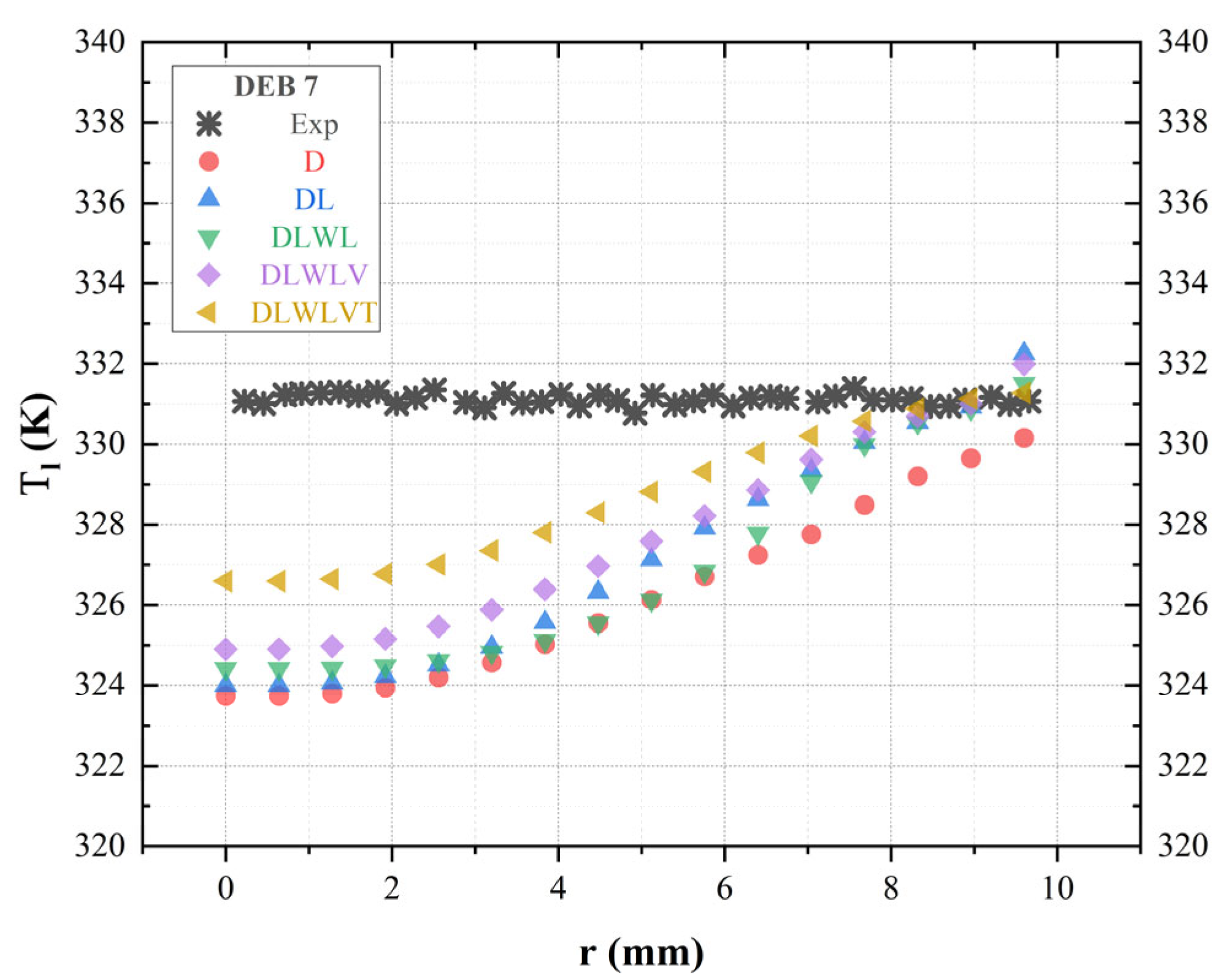
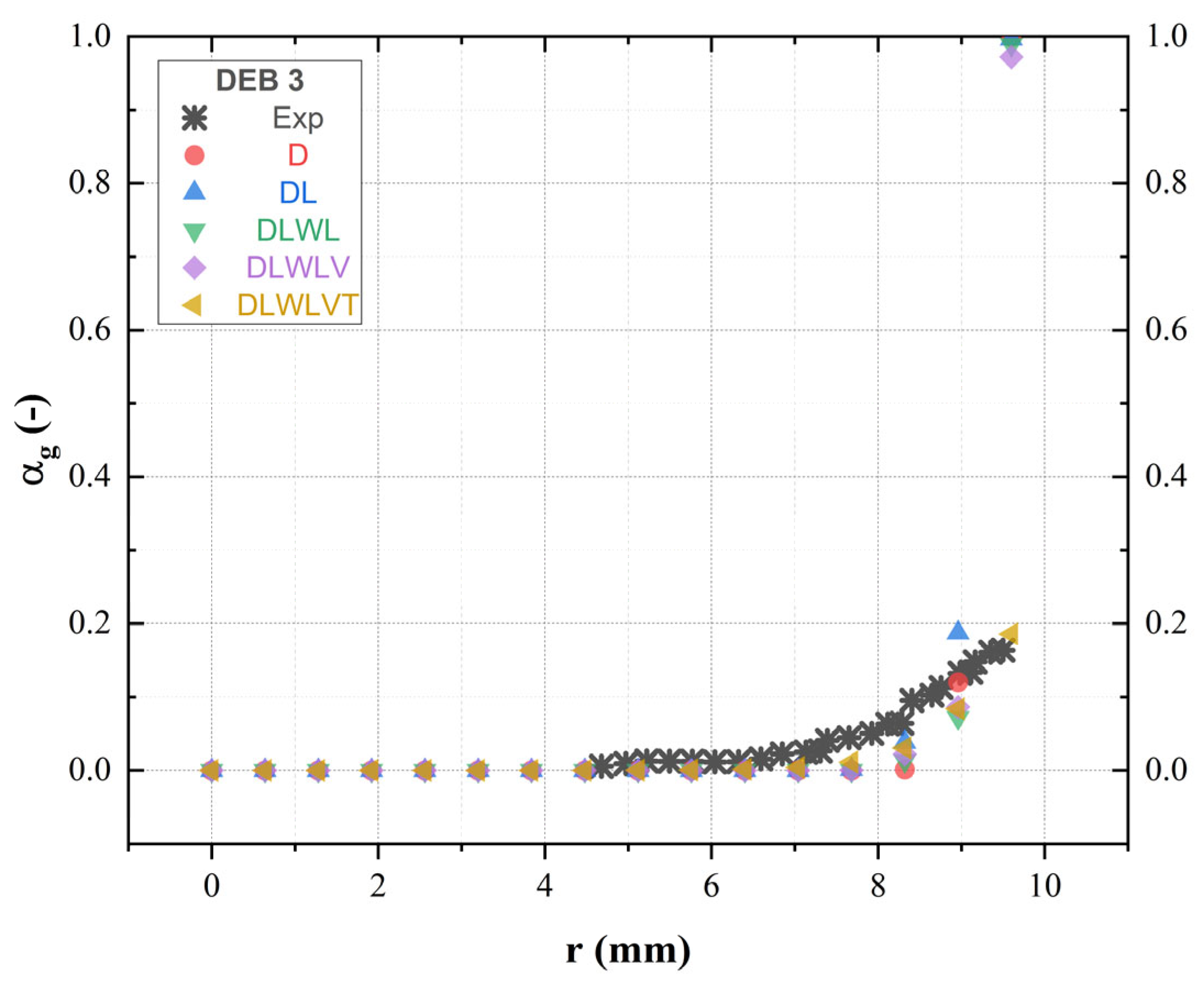
• Analysis of the momentum closure reveals that activating interfacial forces enhances result accuracy, while the exclusion of certain forces detrimentally affects accuracy. The turbulent dispersion force notably influences accuracy, emphasizing the importance of incorporating all five interfacial forces for optimal accuracy.
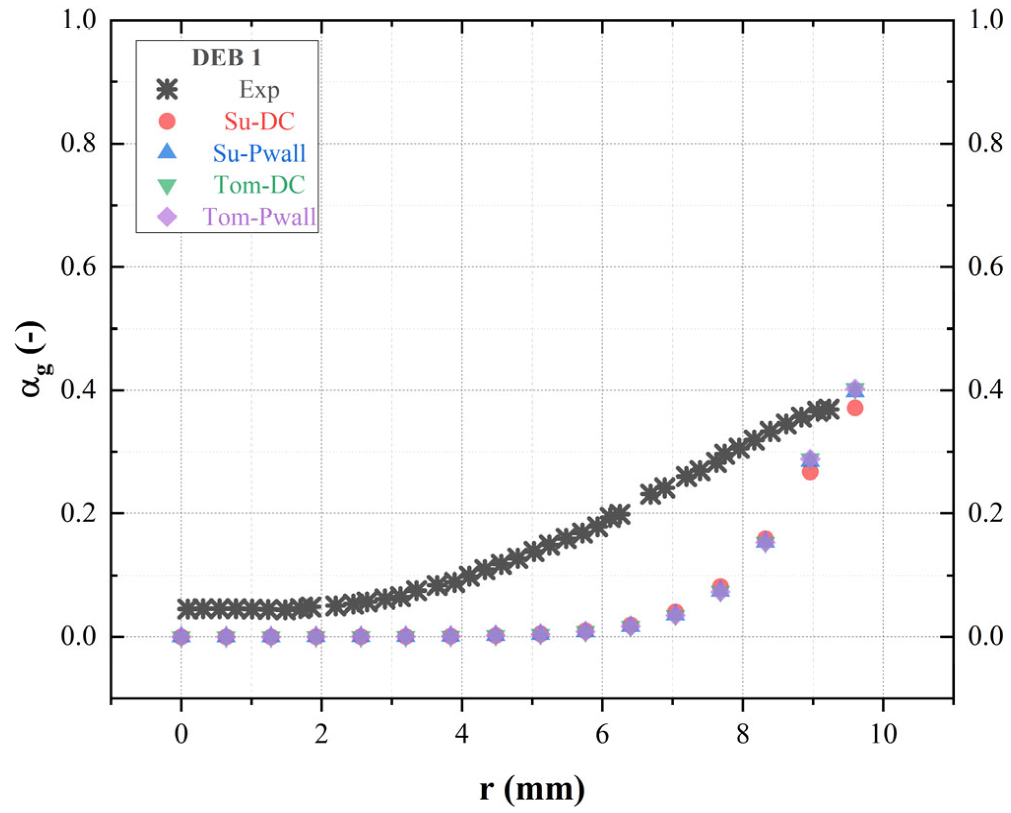
• Sub-closure models for each interfacial force were investigated, highlighting that drag sub-models have a limited impact on temperature but noticeable effects on void fraction. Upon analysis of the simulation outcomes, it was observed that the lift sub-models and the virtual mass force constant demonstrated minimal influence on system behavior. Conversely, a notable impact on both radial profiles of void fraction and liquid temperature was attributed to the turbulence dispersion force constant.
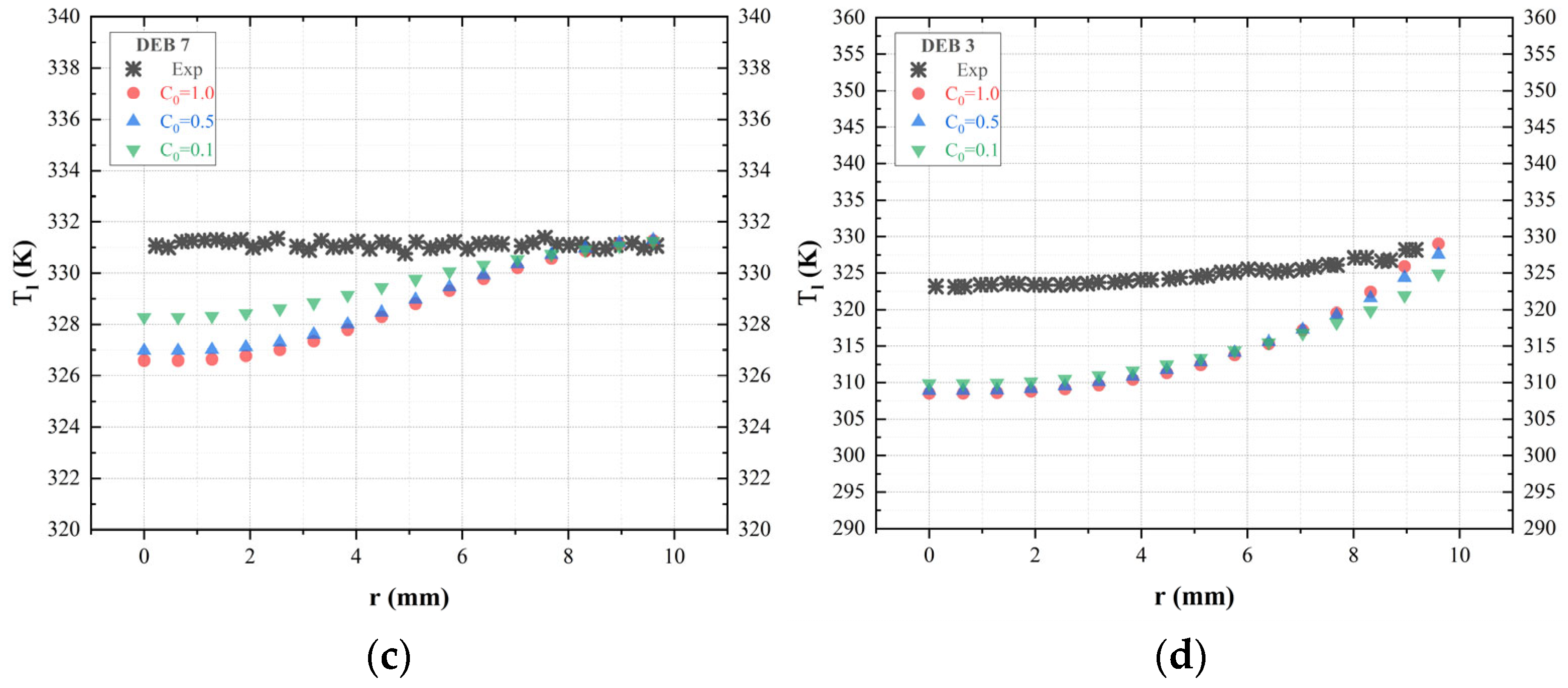
• Incorporating the population balance approach, sensitivity analyses for coalescence and breakage factors were conducted using two different size distribution models (S-Gamma and A MuSigG). These parameters significantly influence momentum exchange within the flow phase and impact the spatial distribution of bubbles. Adjustment of efficiency constants associated with break up and coalescence kernels is deemed crucial based on the analysis of the comparisons observed.

In summary, the present study provides an original comprehensive examination of two-phase CFD refrigerant flow boiling. The study was conducted using refrigerant, not water, and was validated by experiments involving boiling (DEBORA) rather than a liquid/gas mixture, including different subcooling at the inlet. The analysis of different models and their comparison with experimental local data revealed the influence, impact and sensitivity of the key models: boiling closure, momentum closure, and population balance. This analysis and comparison ultimately contribute to a deeper understanding of the underlying phenomena and the development of more accurate models for such systems.

Future work will include 3D simulations to investigate the influence of gravity on the evaporation section at various inclination angles.

References

1. Swanson, T.D.; Birur, G.C. NASA Thermal Control Technologies for Robotic Spacecraft. Appl. Therm. Eng. 2003, 23, 1055–1065. [Google Scholar] [CrossRef]
2. Kunkelmann, C.; Stephan, P. CFD Simulation of Boiling Flows Using the Volume-of-Fluid Method within OpenFOAM. Numer. Heat Transf. Part A Appl. 2009, 56, 631–646. [Google Scholar] [CrossRef]
3. Kunkelmann, C.; Stephan, P. Numerical Simulation of the Transient Heat Transfer during Nucleate Boiling of Refrigerant HFE-7100. Int. J. Refrig. 2010, 33, 1221–1228. [Google Scholar] [CrossRef]
4. Magnini, M.; Thome, J.R. A CFD Study of the Parameters Influencing Heat Transfer in Microchannel Slug Flow Boiling. Int. J. Therm. Sci. 2016, 110, 119–136. [Google Scholar] [CrossRef]
5. Magnini, M.; Matar, O.K. Numerical Study of the Impact of the Channel Shape on Microchannel Boiling Heat Transfer. Int. J. Heat Mass Transf. 2020, 150, 119322. [Google Scholar] [CrossRef]
6. Liu, Q.; Wang, W.; Palm, B. A Numerical Study of the Transition from Slug to Annular Flow in Micro-Channel Convective Boiling. Appl. Therm. Eng. 2017, 112, 73–81. [Google Scholar] [CrossRef]
7. Kurul, N.; Podowski, M.Z. Multidimensional Effects in Forced Convection Subcooled Boiling. In Proceedings of the International Heat Transfer Conference 9, Jerusalem, Israel, 19–24 August 1990; Begellhouse: Jerusalem, Israel, 1990; pp. 21–26. [Google Scholar]
8. Yao, W.; Morel, C. Volumetric Interfacial Area Prediction in Upward Bubbly Two-Phase Flow. Int. J. Heat Mass Transf. 2004, 47, 307–328. [Google Scholar] [CrossRef]
9. Yeoh, G.H.; Tu, J.Y. Two-Fluid and Population Balance Models for Subcooled Boiling Flow. Appl. Math. Model. 2006, 30, 1370–1391. [Google Scholar] [CrossRef]
10. Končar, B.; Matkovič, M. Simulation of Turbulent Boiling Flow in a Vertical Rectangular Channel with One Heated Wall. Nucl. Eng. Des. 2012, 245, 131–139. [Google Scholar] [CrossRef]
11. Yun, B.-J.; Splawski, A.; Lo, S.; Song, C.-H. Prediction of a Subcooled Boiling Flow with Advanced Two-Phase Flow Models. Nucl. Eng. Des. 2012, 253, 351–359. [Google Scholar] [CrossRef]
12. Krepper, E.; Rzehak, R. CFD for Subcooled Flow Boiling: Simulation of DEBORA Experiments. Nucl. Eng. Des. 2011, 241, 3851–3866. [Google Scholar] [CrossRef]
13. Adrian, T.; Vegendla, P.; Obabko, A.; Tomboulides, A.; Fischer, P.; Marin, O.; Merzari, E. Modeling of Two-Phase Flow in a BWR Fuel Assembly with a Highly-Scalable CFD Code. In Proceedings of the 16th International Topical Meeting on Nuclear Reactor Thermal Hydraulics (NURETH-16), Chicago, IL, USA, 30 August–4 September 2015. [Google Scholar]
14. Thakrar, R.; Murallidharan, J.; Walker, S.P. Simulations of High-Pressure Subcooled Boiling Flows in Rectangular Channels. In Proceedings of the 16th International Topical Meeting on Nuclear Reactor Thermal Hydraulics, Chicago, IL, USA, 30 August–4 September 2015. [Google Scholar]
15. Yang, G.; Zhang, W.; Binama, M.; Li, Q.; Cai, W. Review on Bubble Dynamic of Subcooled Flow Boiling-Part b: Behavior and Models. Int. J. Therm. Sci. 2023, 184, 108026. [Google Scholar] [CrossRef]
16. Cheung, S.C.P.; Yeoh, G.H.; Tu, J.Y. On the Numerical Study of Isothermal Vertical Bubbly Flow Using Two Population Balance Approaches. Chem. Eng. Sci. 2007, 62, 4659–4674. [Google Scholar] [CrossRef]
17. Magnaudet, J.; Eames, I. The Motion of High-Reynolds-Number Bubbles in Inhomogeneous Flows. Annu. Rev. Fluid Mech. 2000, 32, 659–708. [Google Scholar] [CrossRef]
18. Yamoah, S.; Martínez-Cuenca, R.; Monrós, G.; Chiva, S.; Macián-Juan, R. Numerical Investigation of Models for Drag, Lift, Wall Lubrication and Turbulent Dispersion Forces for the Simulation of Gas–Liquid Two-Phase Flow. Chem. Eng. Res. Des. 2015, 98, 17–35. [Google Scholar] [CrossRef]
19. Khan, I.; Wang, M.; Zhang, Y.; Tian, W.; Su, G.; Qiu, S. Two-Phase Bubbly Flow Simulation Using CFD Method: A Review of Models for Interfacial Forces. Prog. Nucl. Energy 2020, 125, 103360. [Google Scholar] [CrossRef]
20. Papoulias, D.; Vichansky, A.; Tandon, M. Multi-Fluid Modelling of Bubbly Channel Flows with an Adaptive Multi-Group Population Balance Method. Exp. Comput. Multiph. Flow 2021, 3, 171–185. [Google Scholar] [CrossRef]
21. Ramkrishna, D. Population Balances: Theory and Applications to Particulate Systems in Engineering; Elsevier: Amsterdam, The Netherlands, 2000. [Google Scholar]
22. Hu, G.; Ma, Y.; Liu, Q. Evaluation on Coupling of Wall Boiling and Population Balance Models for Vertical Gas-Liquid Subcooled Boiling Flow of First Loop of Nuclear Power Plant. Energies 2021, 14, 7357. [Google Scholar] [CrossRef]
23. Gupta, A.; Roy, S. Euler–Euler Simulation of Bubbly Flow in a Rectangular Bubble Column: Experimental Validation with Radioactive Particle Tracking. Chem. Eng. J. 2013, 225, 818–836. [Google Scholar] [CrossRef]
24. Tabib, M.V.; Roy, S.A.; Joshi, J.B. CFD Simulation of Bubble Column—An Analysis of Interphase Forces and Turbulence Models. Chem. Eng. J. 2008, 139, 589–614. [Google Scholar] [CrossRef]
25. Frank, T.; Zwart, P.J.; Krepper, E.; Prasser, H.-M.; Lucas, D. Validation of CFD Models for Mono- and Polydisperse Air–Water Two-Phase Flows in Pipes. Nucl. Eng. Des. 2008, 238, 647–659. [Google Scholar] [CrossRef]
26. Drew, D.; Cheng, L.; Lahey, R.T. The Analysis of Virtual Mass Effects in Two-Phase Flow. Int. J. Multiph. Flow 1979, 5, 233–242. [Google Scholar] [CrossRef]
27. Smith, B.L.; Andreani, M.; Bieder, U.; Ducros, F.; Graffard, E.; Heitsch, M.; Henriksson, M.; Höhne, T.; Houkema, M.; Komen, E. Assessment of CFD Codes for Nuclear Reactor Safety Problems-Revision 2; Organisation for Economic Co-Operation and Development: Paris, France, 2015. [Google Scholar]
28. Lee, T.H.; Park, G.C.; Lee, D.J. Local Flow Characteristics of Subcooled Boiling Flow of Water in a Vertical Concentric Annulus. Int. J. Multiph. Flow 2002, 28, 1351–1368. [Google Scholar] [CrossRef]
29. Roy, R.P.; Velidandla, V.; Kalra, S.P. Velocity Field in Turbulent Subcooled Boiling Flow. J. Heat Transf. 1997, 119, 754–766. [Google Scholar] [CrossRef]
30. Garnier, J.; Manon, E.; Cubizolles, G. Local Measurements on Flow Boiling of Refrigerant 12 in a Vertical Tube. Multiph. Sci. Technol. 2001, 13, 111. [Google Scholar] [CrossRef]
31. Estrada-Perez, C.E.; Hassan, Y.A. PTV Experiments of Subcooled Boiling Flow through a Vertical Rectangular Channel. Int. J. Multiph. Flow 2010, 36, 691–706. [Google Scholar] [CrossRef]
32. Cheung, S.C.P.; Vahaji, S.; Yeoh, G.H.; Tu, J.Y. Modeling Subcooled Flow Boiling in Vertical Channels at Low Pressures—Part 1: Assessment of Empirical Correlations. Int. J. Heat Mass Transf. 2014, 75, 736–753. [Google Scholar] [CrossRef]
33. Murallidharan, J.S.; Prasad, B.V.S.S.S.; Patnaik, B.S.V.; Hewitt, G.F.; Badalassi, V. CFD Investigation and Assessment of Wall Heat Flux Partitioning Model for the Prediction of High Pressure Subcooled Flow Boiling. Int. J. Heat Mass Transf. 2016, 103, 211–230. [Google Scholar] [CrossRef]
34. Krepper, E.; Končar, B.; Egorov, Y. CFD Modelling of Subcooled Boiling—Concept, Validation and Application to Fuel Assembly Design. Nucl. Eng. Des. 2007, 237, 716–731. [Google Scholar] [CrossRef]
35. Bartolomei, G.G.; Chanturiya, V.M. Experimental Study of True Void Fraction When Boiling Subcooled Water in Vertical Tubes. Therm. Eng. 1967, 14, 123–128. [Google Scholar]
36. Brooks, C.S.; Silin, N.; Hibiki, T.; Ishii, M. Experimental Investigation of Bubble Departure Diameter and Bubble Departure Frequency in Subcooled Flow Boiling in a Vertical Annulus. In Proceedings of the Volume 2: Heat Transfer Enhancement for Practical Applications; Heat and Mass Transfer in Fire and Combustion Heat Transfer in Multiphase Systems; Heat and Mass Transfer in Biotechnology. American Society of Mechanical Engineers: Minneapolis, MN, USA, 2013; p. V002T07A045. [Google Scholar]
37. Lemmert, M.; Chawla, J.M. Influence of Flow Velocity on Surface Boiling Heat Transfer Coefficient. Heat Transf. Boil. 1977, 237, 247. [Google Scholar]
38. Hibiki, T.; Ishii, M. Active Nucleation Site Density in Boiling Systems. Int. J. Heat Mass Transf. 2003, 46, 2587–2601. [Google Scholar] [CrossRef]
39. Tolubinsky, V.I.; Kostanchuk, D.M. Vapour Bubbles Growth Rate and Heat Transfer Intensity at Subcooled Water Boiling. In Proceedings of the International Heat Transfer Conference 4, Paris, France, 31 September–5 September 1970; Begellhouse: Paris-Versailles, France, 1970; pp. 1–11. [Google Scholar]
40. Kocamustafaogullari, G. Pressure Dependence of Bubble Departure Diameter for Water. Int. Commun. Heat Mass Transf. 1983, 10, 501–509. [Google Scholar] [CrossRef]
41. Cole, R. A Photographic Study of Pool Boiling in the Region of the Critical Heat Flux. AIChE J. 1960, 6, 533–538. [Google Scholar] [CrossRef]
42. Krepper, E.; Rzehak, R.; Lifante, C.; Frank, T. CFD for Subcooled Flow Boiling: Coupling Wall Boiling and Population Balance Models. Nucl. Eng. Des. 2013, 255, 330–346. [Google Scholar] [CrossRef]
43. Cong, T.; Lv, X.; Zhang, X.; Zhang, R. Investigation on the Effects of Model Uncertainties on Subcooled Boiling. Ann. Nucl. Energy 2018, 121, 487–500. [Google Scholar] [CrossRef]
44. Wang, Q.; Yao, W. Computation and Validation of the Interphase Force Models for Bubbly Flow. Int. J. Heat Mass Transf. 2016, 98, 799–813. [Google Scholar] [CrossRef]
45. Gu, J.; Wang, Q.; Wu, Y.; Lyu, J.; Li, S.; Yao, W. Modeling of Subcooled Boiling by Extending the RPI Wall Boiling Model to Ultra-High Pressure Conditions. Appl. Therm. Eng. 2017, 124, 571–584. [Google Scholar] [CrossRef]
46. Bartolomei, G.G.; Brantov, V.G.; Molochnikov, Y.S.; Kharitonov, Y.V.; Solodkii, V.A.; Batashova, G.N.; Mikhailov, V.N. An Experimental Investigation of True Volumetric Vapor Content with Subcooled Boiling in Tubes. Therm. Eng. 1982, 29, 132–135. [Google Scholar]
47. Gray, G.S.; Ormiston, S.J. A Comparative Study of Closure Relations for CFD Modelling of Bubbly Flow in a Vertical Pipe. OJFD 2021, 11, 98–134. [Google Scholar] [CrossRef]
48. Yang, C.-Y.; Nalbandian, H.; Lin, F.-C. Flow Boiling Heat Transfer and Pressure Drop of Refrigerants HFO-1234yf and HFC-134a in Small Circular Tube. Int. J. Heat Mass Transf. 2018, 121, 726–735. [Google Scholar] [CrossRef]
49. Manon, E. Contribution à l’analyse et à La Modélisation Locale Des Écoulements Bouillants Sous-Saturés Dans Les Conditions Des Réacteurs à Eau Sous Pression; Ecole centrale de Paris: Châtenay-Malabry, France, 2000. [Google Scholar]
50. Ishii, M. Thermo-Fluid Dynamic Theory of Two-Phase Flow. NASA STI/Recon Tech. Rep. A 1975, 75, 29657. [Google Scholar]
51. Drew, D.A.; Stephen, L.P. Theory of Multicomponent Fluids; Springer Science & Business Media: Berlin, Germany, 2006; Volume 135. [Google Scholar]
52. Wallis, G.B. One-Dimensional Two-Phase Flow; Courier Dover Publications: Mineola, NY, USA, 2020. [Google Scholar]
53. Kurul, N.; Podowski, M.Z. On the Modeling of Multidimensional Effects in Boiling Channels. In Proceedings of the 27th National Heat Transfer Conference, Minneapolis, MN, USA, 28–31 July 1991. [Google Scholar]
54. Benjamin, R.J.; Balakrishnan, A.R. Nucleation Site Density in Pool Boiling of Binary Mixtures: Effect of Surface Micro-roughness and Surface and Liquid Physical Properties. Can. J. Chem. Eng. 1997, 75, 1080–1089. [Google Scholar] [CrossRef]
55. Gao, Y.; Shao, S.; Xu, H.; Zou, H.; Tang, M.; Tian, C. Numerical Investigation on Onset of Significant Void during Water Subcooled Flow Boiling. Appl. Therm. Eng. 2016, 105, 8–17. [Google Scholar] [CrossRef]
56. Leong, K.C.; Ho, J.Y.; Wong, K.K. A Critical Review of Pool and Flow Boiling Heat Transfer of Dielectric Fluids on Enhanced Surfaces. Appl. Therm. Eng. 2017, 112, 999–1019. [Google Scholar] [CrossRef]
57. Podowski, M.Z.; Podowski, R.M. Mechanistic Multidimensional Modeling of Forced Convection Boiling Heat Transfer. Sci. Technol. Nucl. Install. 2009, 2009, 387020. [Google Scholar] [CrossRef]
58. Ünal, H.C. Maximum Bubble Diameter, Maximum Bubble-Growth Time and Bubble-Growth Rate during the Subcooled Nucleate Flow Boiling of Water up to 17.7 MN/M2. Int. J. Heat Mass Transf. 1976, 19, 643–649. [Google Scholar] [CrossRef]
59. Euh, D.; Ozar, B.; Hibiki, T.; Ishii, M.; Song, C.-H. Characteristics of Bubble Departure Frequency in a Low-Pressure Subcooled Boiling Flow. J. Nucl. Sci. Technol. 2010, 47, 608–617. [Google Scholar] [CrossRef]
60. Ishii, M.; Zuber, N. Drag Coefficient and Relative Velocity in Bubbly, Droplet or Particulate Flows. AIChE J. 1979, 25, 843–855. [Google Scholar] [CrossRef]
61. Akbar, M.H.b.M.; Hayashi, K.; Lucas, D.; Tomiyama, A. Effects of Inlet Condition on Flow Structure of Bubbly Flow in a Rectangular Column. Chem. Eng. Sci. 2013, 104, 166–176. [Google Scholar] [CrossRef]
62. Rzehak, R.; Kriebitzsch, S. Multiphase CFD-Simulation of Bubbly Pipe Flow: A Code Comparison. Int. J. Multiph. Flow 2015, 68, 135–152. [Google Scholar] [CrossRef]
63. Schiller, L.; Maumann, A. Uber Die Grundlegenden Berechnungen Bei Der Schwerkraftaufbereitung. Z. Des Vereines Dtsch. Ingenieure 1933, 77, 318–321. [Google Scholar]
64. Rusche, H.; Issa, R.I. The Effect of Voidage on the Drag Force on Particles, Droplets and Bubbles in Dispersed Two-Phase Flow. In Proceedings of the Japanese European Two-Phase Flow Meeting, Tshkuba, Japan, 25–29 September 2000. [Google Scholar]
65. Bozzano, G.; Dente, M. Shape and Terminal Velocity of Single Bubble Motion: A Novel Approach. Comput. Chem. Eng. 2001, 25, 571–576. [Google Scholar] [CrossRef]
66. Chhabra, R.P. Bubbles, Drops, and Particles in Non-Newtonian Fluids, 2nd ed.; CRC Press: Boca Raton, FL, USA, 2006; ISBN 978-0-429-07480-6. [Google Scholar]
67. Tomiyama, A.; Kataoka, I.; Zun, I.; Sakaguchi, T. Drag Coefficients of Single Bubbles under Normal and Micro Gravity Conditions. JSME Int. J. Ser. B 1998, 41, 472–479. [Google Scholar] [CrossRef]
68. Wang, D.M. Modelling of Bubbly Flow in a Sudden Pipe Expansion; Technical Report II-34; BRITE/EuRam Project BE-4098; European Union: Luxembourg, 1994. [Google Scholar]
69. Behzadi, A.; Issa, R.I.; Rusche, H. Modelling of Dispersed Bubble and Droplet Flow at High Phase Fractions. Chem. Eng. Sci. 2004, 59, 759–770. [Google Scholar] [CrossRef]
70. Auton, T.R.; Hunt, J.C.R.; Prud’Homme, M. The Force Exerted on a Body in Inviscid Unsteady Non-Uniform Rotational Flow. J. Fluid Mech. 1988, 197, 241–257. [Google Scholar] [CrossRef]
71. Tomiyama, A.; Tamai, H.; Zun, I.; Hosokawa, S. Transverse Migration of Single Bubbles in Simple Shear Flows. Chem. Eng. Sci. 2002, 57, 1849–1858. [Google Scholar] [CrossRef]
72. Sugrue, R.M. A Robust Momentum Closure Approach for Multiphase Computational Fluid Dynamics Applications. Ph.D. Thesis, Massachusetts Institute of Technology, Cambridge, MA, USA, 2017. [Google Scholar]
73. Shaver, D.R.; Podowski, M.Z. Modeling of Interfacial Forces for Bubbly Flows in Subcooled Boiling Conditions. Trans. Am. Nucl. Soc. 2015, 113, 1368–1371. [Google Scholar]
74. Moraga, F.J.; Larreteguy, A.E.; Drew, D.A.; Lahey, R.T. Assessment of Turbulent Dispersion Models for Bubbly Flows in the Low Stokes Number Limit. Int. J. Multiph. Flow 2003, 29, 655–673. [Google Scholar] [CrossRef]
75. Mukhopadhyay, S.; Nimbalkar, G. Fundamental Study on Chaotic Transition of Two-Phase Flow Regime and Free Surface Instability in Gas Deaeration Process. Exp. Comput. Multiph. Flow 2021, 3, 258–288. [Google Scholar] [CrossRef]
76. Lamb, H. Hydrodynamics; Dover Publications: New York, NY, USA, 1945; Volume 445. [Google Scholar]
77. Zuber, N. On the Dispersed Two-Phase Flow in the Laminar Flow Regime. Chem. Eng. Sci. 1964, 19, 897–917. [Google Scholar] [CrossRef]
78. Antal, S.P.; Lahey, R.T.; Flaherty, J.E. Analysis of Phase Distribution in Fully Developed Laminar Bubbly Two-Phase Flow. Int. J. Multiph. Flow 1991, 17, 635–652. [Google Scholar] [CrossRef]
79. Lo, S.; Rao, P. Modelling of Droplet Breakup and Coalescence in an Oil-Water Pipeline. In Proceedings of the 6th International Conference on Multiphase Flow, ICMF 2007, Leipzig, Germany, 9–13 July 2007. [Google Scholar]
80. Lo, S.; Zhang, D. Modelling of Break-up and Coalescence in Bubbly Two-Phase Flows. J. Comput. Multiph. Flows 2009, 1, 23–38. [Google Scholar] [CrossRef]
81. Lo, S. Application of Population Balance to CFD Modeling of Bubbly Flow Via the MUSIG Model; AEA Technology: Carlsbad, CA, USA, 1996. [Google Scholar]
82. Tsouris, C.; Tavlarides, L.L. Breakage and Coalescence Models for Drops in Turbulent Dispersions. AIChE J. 1994, 40, 395–406. [Google Scholar] [CrossRef]
83. Luo, H. Coalescence, Breakup and Liquid Circulation in Bubble Column Reactors. Ph.D. Thesis, Norwegian Institute of Technology, Trondheim, Norway, 1993. [Google Scholar]
84. Vlček, D.; Sato, Y. Sensitivity Analysis for Subcooled Flow Boiling Using Eulerian CFD Approach. Nucl. Eng. Des. 2023, 405, 112194. [Google Scholar] [CrossRef]
85. Yeo, I.; Lee, S. 2D Computational Investigation into Transport Phenomena of Subcooled and Saturated Flow Boiling in Large Length to Diameter Ratio Micro-Channel Heat Sinks. Int. J. Heat Mass Transf. 2022, 183, 122128. [Google Scholar] [CrossRef]
86. Wei, L.; Pan, L.; Liu, H.; Ren, Q.; He, H.; Cen, K.; Wang, D.; Yan, M. Assessment of Wall Heat Flux Partitioning Model for Two-Phase CFD. Nucl. Eng. Des. 2022, 390, 111693. [Google Scholar] [CrossRef]
87. Siemens Digital Industries Software. Simcenter STAR-CCM+ User Guide, Version 18.02.010; Siemens Digital Industries Software: Plano, TX, USA, 2023. [Google Scholar]
Figure 1. Illustration of EE two-fluid model coupled with wall boiling model, population balance model and interfacial force model for gas–liquid flow [22].
Energies 17 04225 g001
Figure 2. The 2D computational domain and boundary conditions.
Energies 17 04225 g002
Figure 3. Grid sensitivity investigation: (a) based on axial division, radial void fraction (grid size: V1—30 × 100, V2—30 × 300, V3—30 × 600, V4—30 × 900) profile for DEB1 case; (b) based on radial division, radial void fraction profile for DEB3 case; (c) radial liquid temperature profile for DEB7 case; and (d) axial wall temperature along tube wall for DEB1 case (grid size: G1—10 × 100, G2—20 × 200, G3—30 × 300, G4—40 × 400, G5—50 × 500).
Energies 17 04225 g003
Figure 4. Comparison under various combinations of bubble departure diameter and active nucleation site density of: (a) axial distribution of wall temperatures with the experimental dataset of DEBORA (DEB7); (b) radial profile of liquid temperature with the experimental dataset of DEBORA (DEB7); (c,d) radial void fraction profile with the experimental dataset of DEBORA (DEB1) and (DEB3).
Energies 17 04225 g004
Figure 5. Comparison of axial distribution of wall temperature along the tube with the experimental dataset of DEBORA (DEB1) under various combinations of interphase forces. (D—drag force, L—lift force, WL—wall lubrication force, V—virtual mass force, T—turbulent dispersion force).
Energies 17 04225 g005
Figure 6. Comparison of radial profile of liquid temperature with the experimental dataset of DEBORA (DEB7) under various combinations of interphase forces. (D—drag force, L—lift force, WL—wall lubrication force, V—virtual mass force, T—turbulent).
Energies 17 04225 g006
Figure 7. Comparison of radial profile of void fraction with the experimental dataset of DEBORA (DEB3) under various combinations of interphase forces. (D—drag force, L—lift force, WL—wall lubrication force, V—virtual mass force, T—turbulent dispersion force).
Energies 17 04225 g007
Figure 8. Comparison with the experimental dataset of DEB1 of radial void fraction profile for drag force models.
Energies 17 04225 g008
Figure 9. Comparison of radial void fraction profile for lift force models with the experimental dataset of DEB1 by combination of lift coefficient and the lift correction.
Energies 17 04225 g009
Figure 10. Comparison under different turbulent dispersion coefficient constant values of: (a) and (b)radial void fraction with the experimental dataset of DEBORA (DEB1 and DEB3); (c,d) radial liquid temperature with the experimental dataset of DEBORA (DEB7 and DEB3).
Energies 17 04225 g010aEnergies 17 04225 g010b
Figure 11. Comparison of radial liquid temperature profile with the experimental dataset of DEBORA case 7 under different virtual mass constant values and virtual mass models.
Energies 17 04225 g011
Figure 12. Comparison of radial liquid temperature with the experimental dataset of DEBORA under different combinations of S-Gamma sub-closure models: (a) DEB1; (b) DEB3; and (c) DEB7 ([BK—break up model, CL—coalescence model).
Energies 17 04225 g012
Figure 13. Comparison of radial void fraction with the experimental dataset of DEBORA 7 under different combinations of S-Gamma sub-closure models (BK—break up model, CL—coalescence model).
Energies 17 04225 g013
Figure 14. Comparison of radial void fraction with the experimental dataset of DEBORA 7 under different combinations of A MuSiG sub-closure models (BK—break up model; CL—coalescence model).
Energies 17 04225 g014
Figure 15. DEB1 volume of fraction contours resulting from various combinations of the S-Gamma sub-closure model: (a) no sub-closure model; (b) break up model; (c) coalescence model; and (d) break up model and coalescence model.
Energies 17 04225 g015
Figure 16. DEB1 liquid temperature distribution resulting from various combinations of the S-Gamma sub-closure model: (a) no sub-closure model; (b) break up model; (c) coalescence model; and (d) break up model and coalescence model.
Energies 17 04225 g016
Figure 17. DEB3 volume of fraction contours with break up model and coalescence model: (a) S-Gamma; (b) A MuSiG, liquid temperature contours with break up model and coalescence model; (c) S-Gamma; (d) A MuSiG.
Energies 17 04225 g017