Abstract
Artificial neural networks (ANNs) can be used for accurate heat load forecasting in district heating systems (DHSs). This paper presents an application of a shallow ANN with two hidden layers in the case of a local DHS. The developed model was used to write a simple application in Python 3.10 that can be used in the operation of a district heating plant to carry out a preliminary analysis of heat demand, taking into account the ambient temperature on a given day. The model was trained using the real data from the period 2019–2022. The training was sufficient for the number of 150 epochs. The prediction effectiveness indicator was proposed. In the considered case, the effectiveness of the trained network was 85% and was better in comparison to five different regression models. The developed tool was based on an open-source programming environment and proved its ability to predict heating load.
1. Introduction
District heating systems (DHSs) are commonly used as an effective method forenergy supplies in the residential sector. In total, household energy consumption district heat in 2021 had 8.6% and 18.3% shares in the EU and Poland, respectively [1]. The total length of heating networks in Poland rose by 6.6% between 2012 and 2022 [2], reaching over 25,000 km, of which 96% was located in urban areas [3].
Heat load in DHSs is influenced by numerous factors [4,5]. Hence, for efficient operation of DHS plants, various heat load prediction techniques have been developed during recent decades. In the literature [6,7,8], these techniques are divided into physical-based, data-driven and hybrid methods. The physical-based models produce correlations between heat load and physical input factors (DHS parameters, material characteristics, weather, etc.). As they require a large amount of input data, they are time consuming. Data-driven models use historical energy demand and influencing factors to predict thermal load not requiring physical analysis of DHSs [9]. Taking advantage of this feature, in combination with the use of computer techniques, a wide range of approaches have been developed, especially machine learning solutions [10]. Among others, artificial neural networks (ANNs) are popular due to their good computing time [11], lower complexity in multi-variable issues [12] and easy adaptation to system nonlinearities [13] and various heat load profiles [14].However, despite the rapidly rising number of applications, machine learning and deep learning in DHS applications have still low shares [15]. Therefore, this part of ANN use is of interest.
Most works have focused on the heat load prediction in DHSs applying various ANN-based models using different sets of input variables (Table 1).

Table 1.
Simulation models used in various data-driven forecast methods of DHSs.
In general, the authors mainly compared various machine learning solutions in terms of their prediction accuracy. Wei et al. [32] analysed seven models, concluding that the weather forecasting data mostly influenced model performance. Li et al. [4] proposed an Elman neural network to model heat load using ambient temperature and sunlight factor as input variables. Using the experimental data from a heating company, they achieved a relative error for short-term prediction below 2%.
A different approach was presented by Bujalski et al. [33]. The authors compared results from ANN predictions with those from an exponential regression model with an input ambient air temperature and obtained forecast accuracy of 6.86% and 12.92%, respectively. As more accurate planning of heat or electricity generation is of significant economic importance [34], there is a need to analyse the potential benefits resulting from the use of ANN-based tools in relation to the usually used heat load demand curves.
As presented in Table 1, most of the studies were devoted to 24 h ahead heat-load forecasts based on hourly weather data. The authors focused on a comparison of various ANN-based models. The use of heating curves was not shown, although in our experience these models are often used in numerous low-power facilities. In addition, such objects often do not possess archived reliable hourly data on ambient climate and heat production. But, in practise, only general daily data are available for smaller-capacity facilities. In such cases, the question arises as to whether they can be used to forecast heat production with knowledge of the basic parameter defining ambient conditions, i.e., the air temperature. This is the gap that emerged from the literature analysis presented.
The second task was the use of freely available software. This way, the user was not restricted by the need for specialised commercial software or additional costs. Therefore, Python language (version 3.10) was chosen as it is often used for data analysis and scientific computing. It also contains various packages for machine learning applications [35], which makes this solution cheap and flexible in terms of future development.
This paper aimed to develop a neural network model designed to predict the heat demand produced in a district heating plant and to assess its accuracy in relation to the typical heating curves. The resulting model was used to write a simple application that can be used in the operation of a district heating plant to carry out a forecast of heat demand based on the ambient temperature on a given day.
This paper is structured as follows. In the design section, the process of analysing the obtained data and adapting them to the computational needs of the neural network model is presented and discussed. Then, the process of building the neural network model based on the available libraries, which are briefly presented, is described. Once the prepared model is trained and all validation calculations are performed, an interface is prepared for the heating plant staff. Then, the conclusions are given.
2. Materials and Methods
2.1. Research Strategy
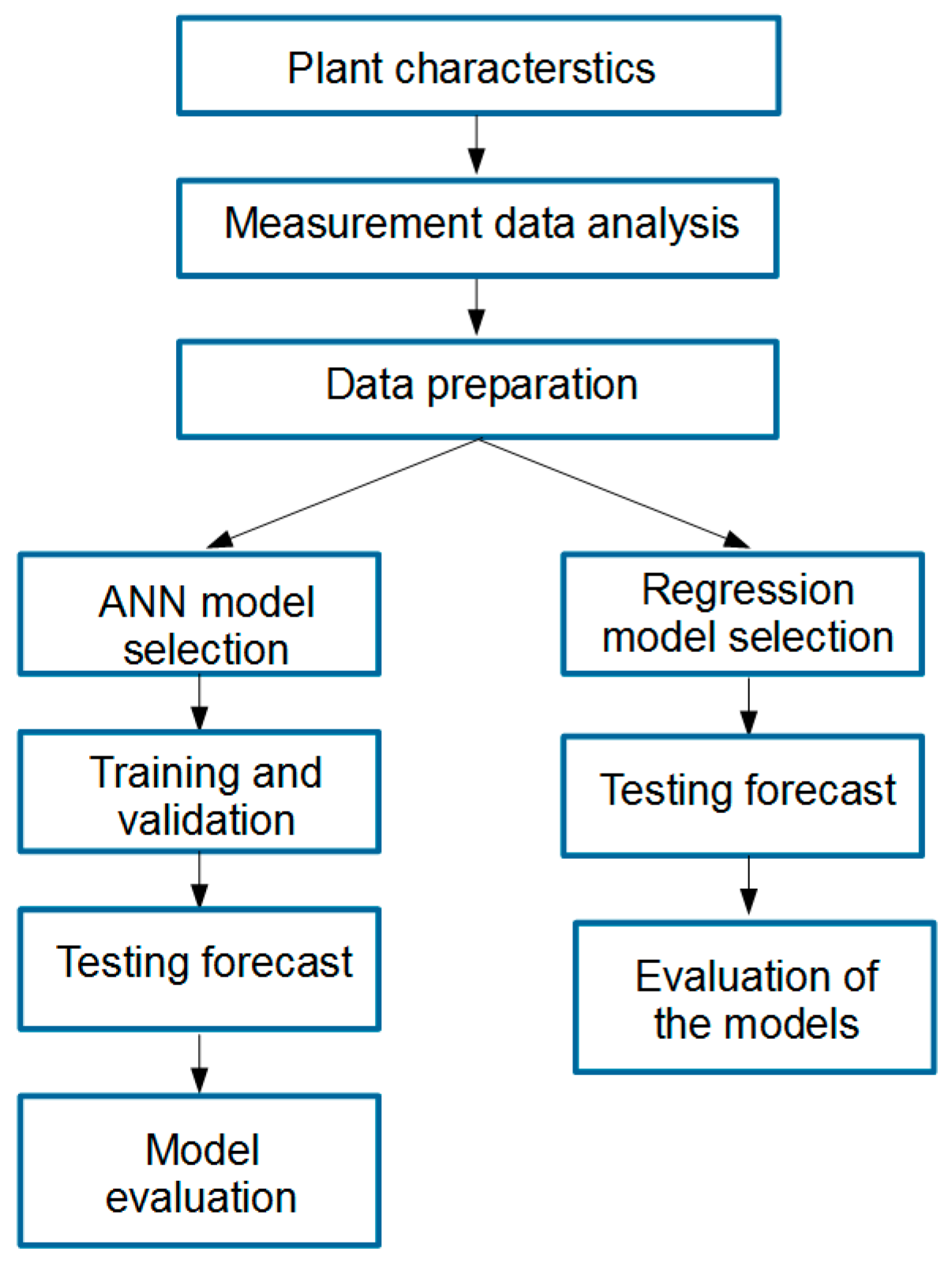
The research algorithm is outlined in Figure 1. After briefly detailing plant characteristics, a measurement data analysis was performed. All variables were outlined and then inconsistencies were identified to prepare the input dataset for further analysis.

Figure 1.
The research algorithm.
In the next step, two kinds of forecasting models were developed and examined. The architecture of the ANN model was selected after a literature review and then several tests and validations were conducted, showing the model’s ability to properly work with the specific input dataset. Finally, it was tested and its quality was evaluated using the proposed performance indicator. Similarly, using the same data, five regression models were developed and then tested. Finally, their comparison was presented.
2.2. Operation Parameters of the Heating Plant
This study uses measurement data obtained in a municipal heating plant located in west Poland. This plant is supplied mostly by natural gas, the consumption of which in 2022 was 2.4 ∙ 106 m3. This is the main fuel used at this heating plant, but it is also possible to use heating oil, the consumption of which in 2022 was 644 m3. In further analysis, daily data from 1 January 2019 to 30 June 2022 were used.
The purpose of a district heating plant is to supply heat to consumers with a system of pipelines. The heat supplied can be determined by measuring the parameters of the district heating network. Water at a set temperature feeds into the network and then returns to the district heating plant at a correspondingly lower temperature. The temperature difference, the mass of water flowing through the network and the specific heat of the water allow for the calculation of the heat that has been discharged into the district heating network.
where
with
Q = m ∙ c ∙ ΔT,
- m—the mass of the water in the heating network, kg;
- ρ—the density of the water, kg/m3;
- c—the specific heat of the water, J/kgK;
- —the mass flow rate of the water in the heating network, kg/s;
- —the volume flow rate of the water in the heating network, kg/s;
- Δτ—the time, s;
- ∆T—the difference between the supply and return temperature, K.
Some important aspects that may be of particular interest to energy engineers are issues such as the parameters of the district heating network, heat losses in the pipeline and ways of feeding the network. The parameters analysed and their influence on the operation of a district heating plant are given in Table 2.

Table 2.
Parameters recorded in the heating plant.
The supply pressure of the heating water at the inlet of a network can be controlled in the range of 0.18–0.70 MPa. This way, it is possible to increase the water mass flow rate. Together with the supply temperature, the heating power of the plant is controlled [36].
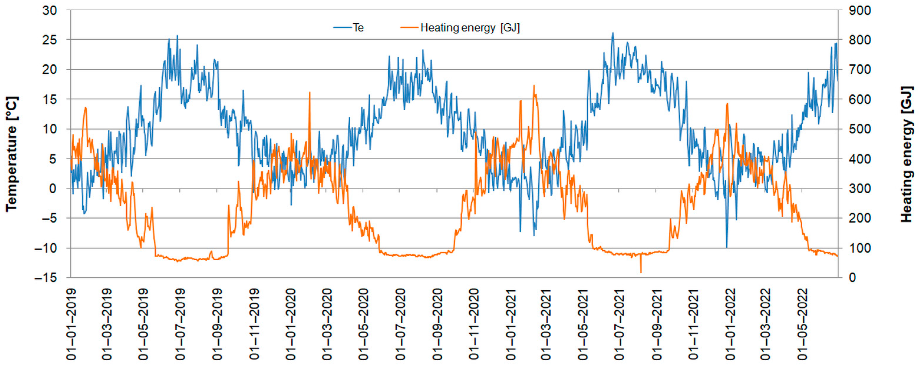
The parameters presented above are mostly strictly dependent on the operation of the plant and it would be pointless to forecast them. For example, the temperature of the heating medium at the return of the network is a result of the supply temperature and the thermal energy transferred to the end-users. After an in-depth analysis, it becomes apparent that the key parameter that affects the heat demand of consumers is the ambient temperature (Figure 2); it was chosen for further analysis.
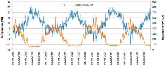
Figure 2.
Ambient temperature and heat production.
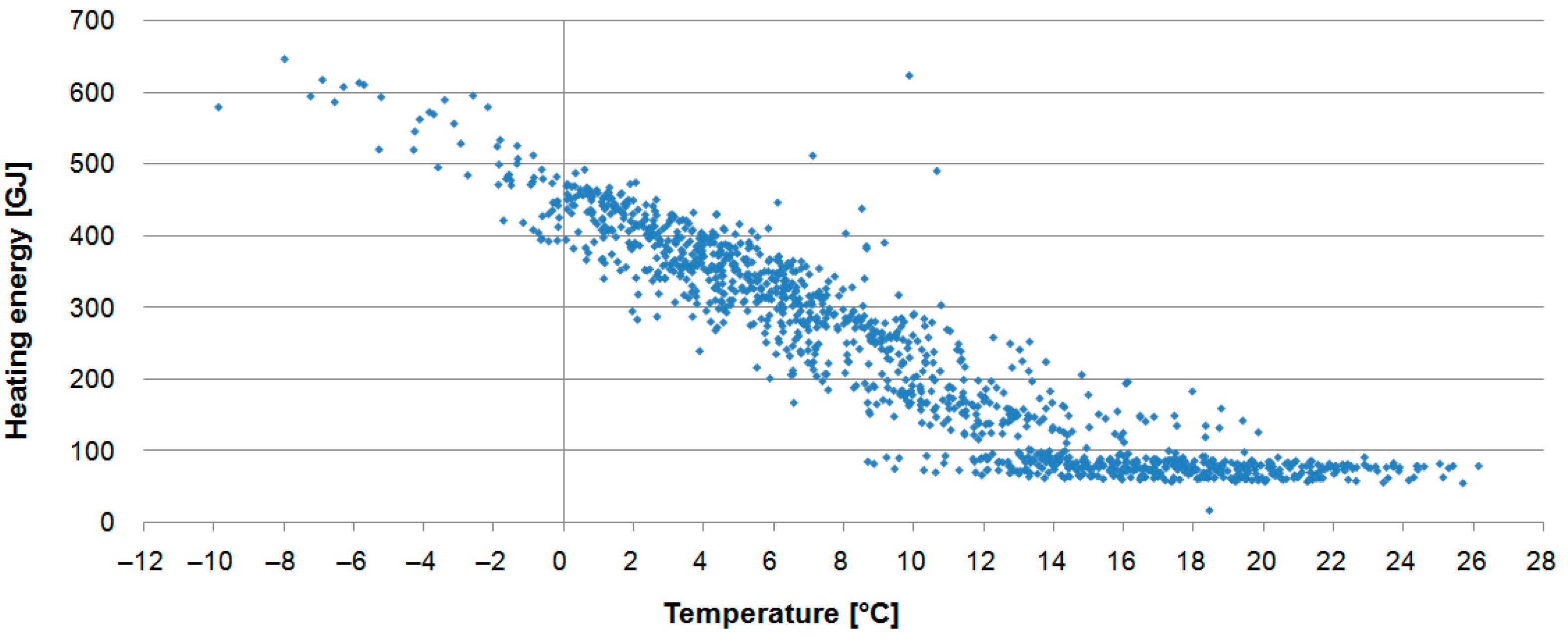
Figure 3 presents the relation between daily heat demand and ambient temperature for the whole analysed period. During the warm season, when buildings connected to the considered network are not heated, there is almost constant heat demand (below 100 GJ),which can be attributed mainly to tap water and small commercial consumers.
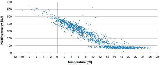
Figure 3.
Heating energy and ambient temperature.
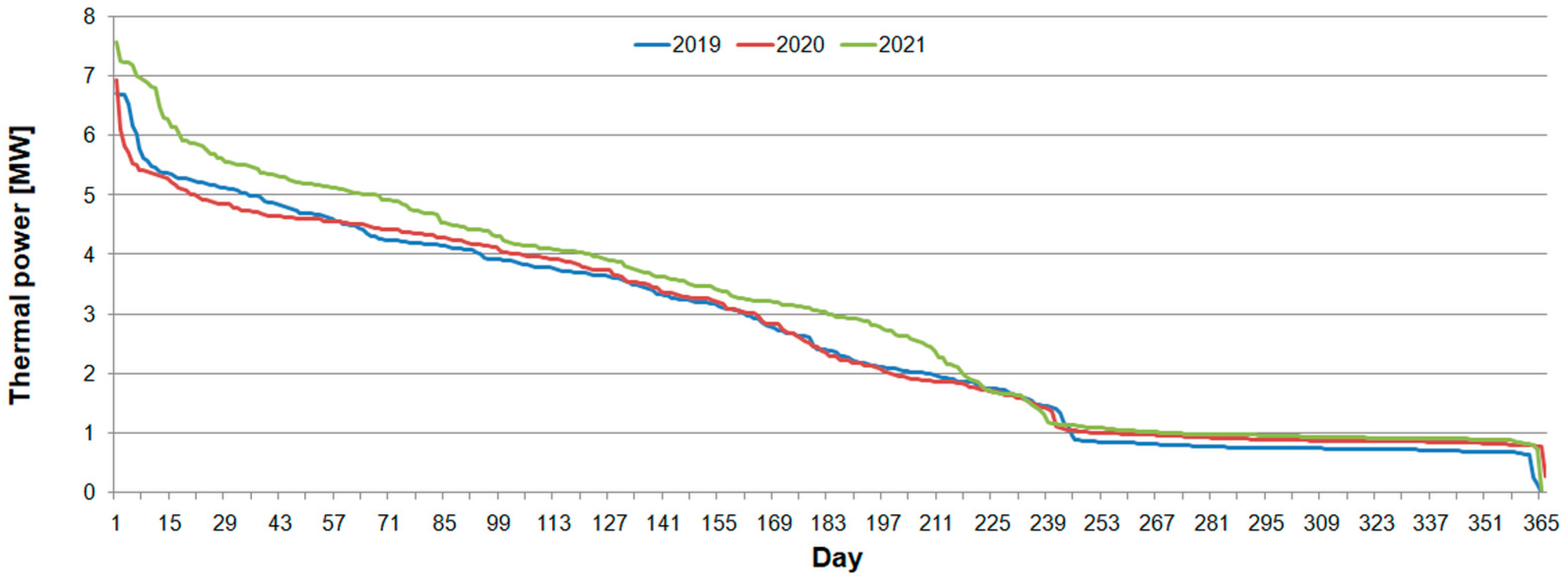
Peak thermal power was 7.6 MW, 7.0 MW and 6.7 MW in 2021, 2020 and 2019, respectively (Figure 4). Despite differences in daily values, the presented heating power duration curves are very similar. Space heating of buildings lasted for about 2/3 of the year, until the 240th day.
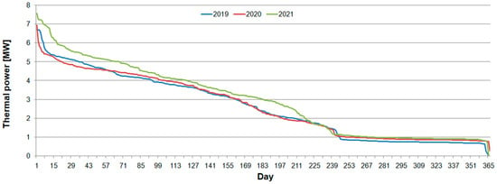
Figure 4.
Daily duration curves of heating power in 2019, 2020 and 2021.
2.3. Input Data Preparation and Preliminary Analysis
The measurement data obtained from the district heating company were prepared in Microsoft Excel 2007 spreadsheets and Excel format spreadsheets, but without consistently using the same data storage format. In order to import the data, it was necessary to organise the data in advance and check the validity of the data types (Table 3). To this end, after data import, information was obtained on what type of data was stored in the consecutive columns. The measurements in all columns except the date column are of the floating-point type, as expected.

Table 3.
Deficiencies in imported data.
Another problem encountered after data import was that unknown values were present in many records. The more significant gaps were observed in the last two columns of the data, i.e., in the operating times of the boilers. Due to the lack of data on the operating principles and operation of the heating block, these data were omitted, and this simplification did not take into account the breakdown of the operation by individual boilers. In the part of the data where the data were complete, the periods were observed when the boilers operated simultaneously or in configurations dependent on service or fault repair. This simplification unfortunately loses the possibility to take into account the relationship between the individual unit and the parameters obtained during the operation of the heating plant. With only 1593 data records available, it was necessary to focus on the most important problem of this issue, which is heat demand forecasting.
The next step in the preliminary analysis of the imported data was to calculate basic statistical information on each of the variables, such as the sum, mean value, median value, standard deviations, minimum value, maximum value, and percentages in the ranges presented (Table 4).

Table 4.
Statistical analysis of the selected variables in the source files.
Preliminary analysis of the data leads to the conclusion that the minimum values of the presented columns should not be equal to 0. Such a situation is possible, but not during the normal operation of the heat plant. Therefore, all zero records were deleted.
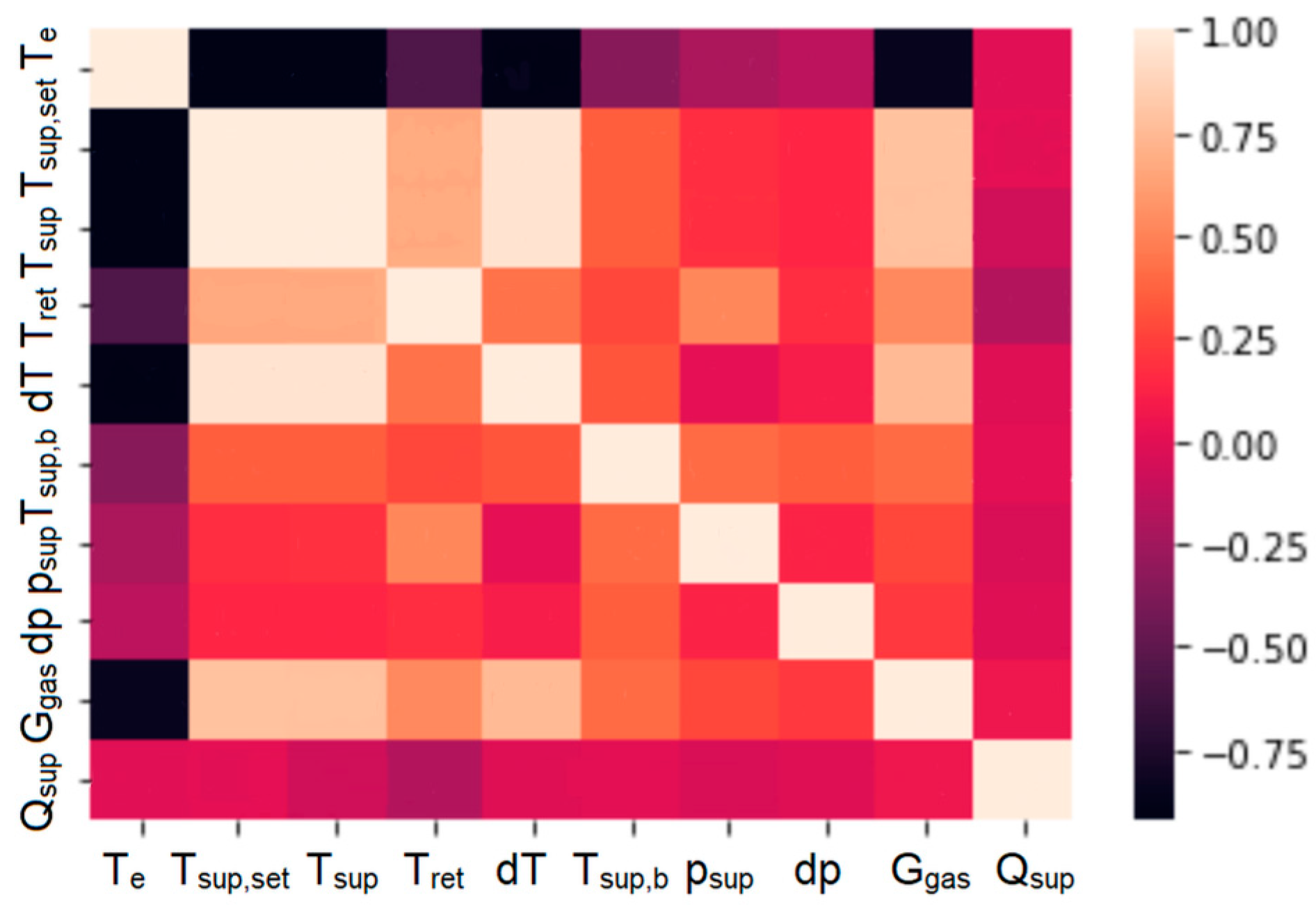
After this operation, the set of records was reduced to 1534. Next, to determine the relationship between the individual data columns, a heat map was generated using the SeaBorn library. This map (Figure 5) indicates the degree of correlation between the data as determined by the value of Pearson’s correlation coefficient.
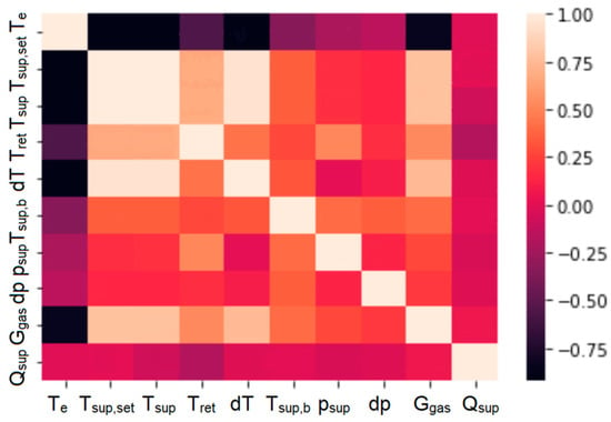
Figure 5.
The Pearson correlation coefficient matrix plot for the heat load and influencing factors.
The bars in black represent correlations close to a value of −1, i.e., as the value of one parameter increases, the other decreases. The white boxes represent correlations close to 1, i.e., where, as one parameter increases, the other also increases.
The data presented above include only measured values. Sampling was carried out once a day, which resulted in each measurement being linked to a reading date. Based on the date, two additional columns were created with the day of the week (Monday–Sunday), with values from 0 to 6 corresponding to the day of the week, and a column with the month name (January–December) with values from 1 to 12.
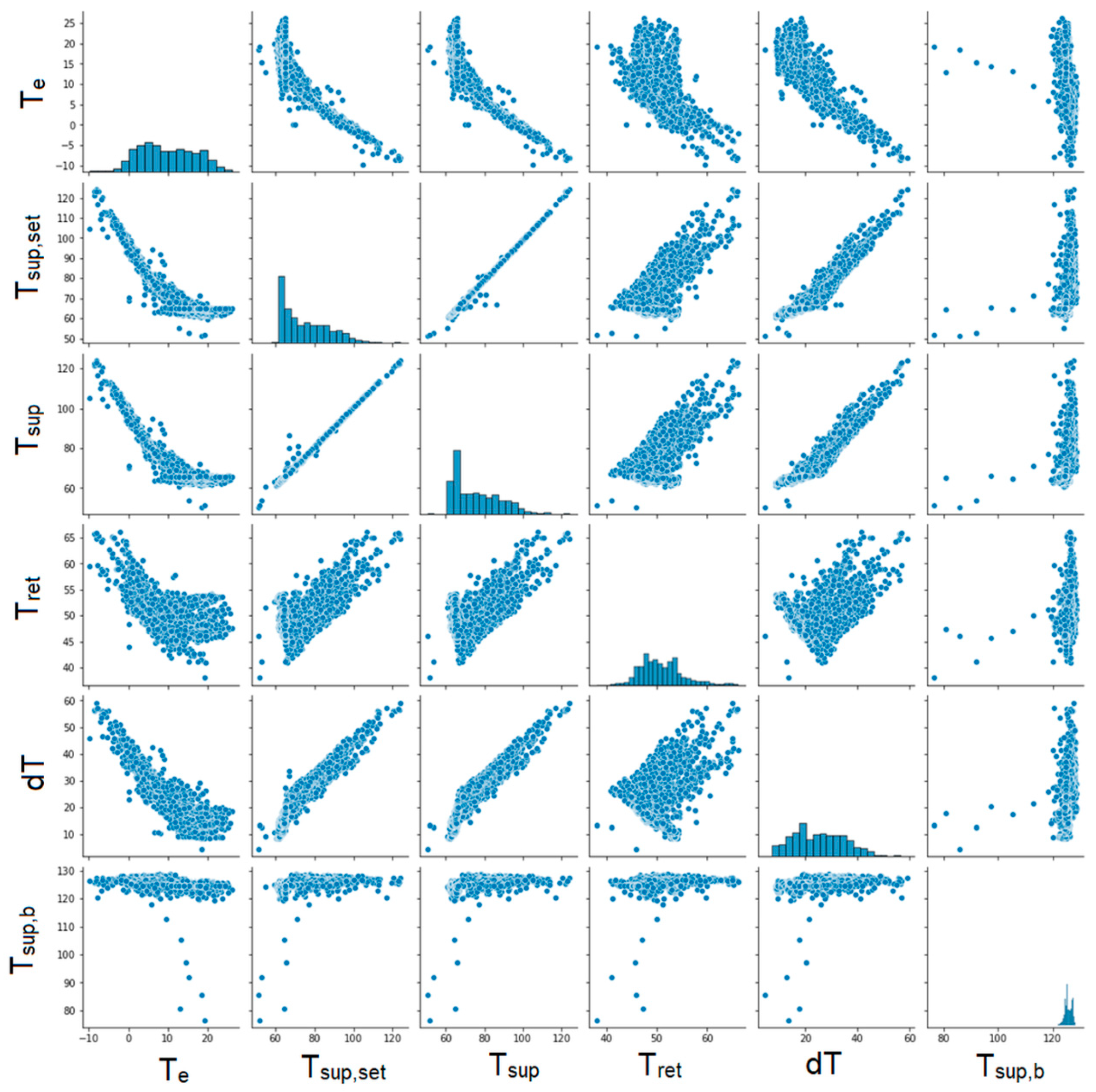
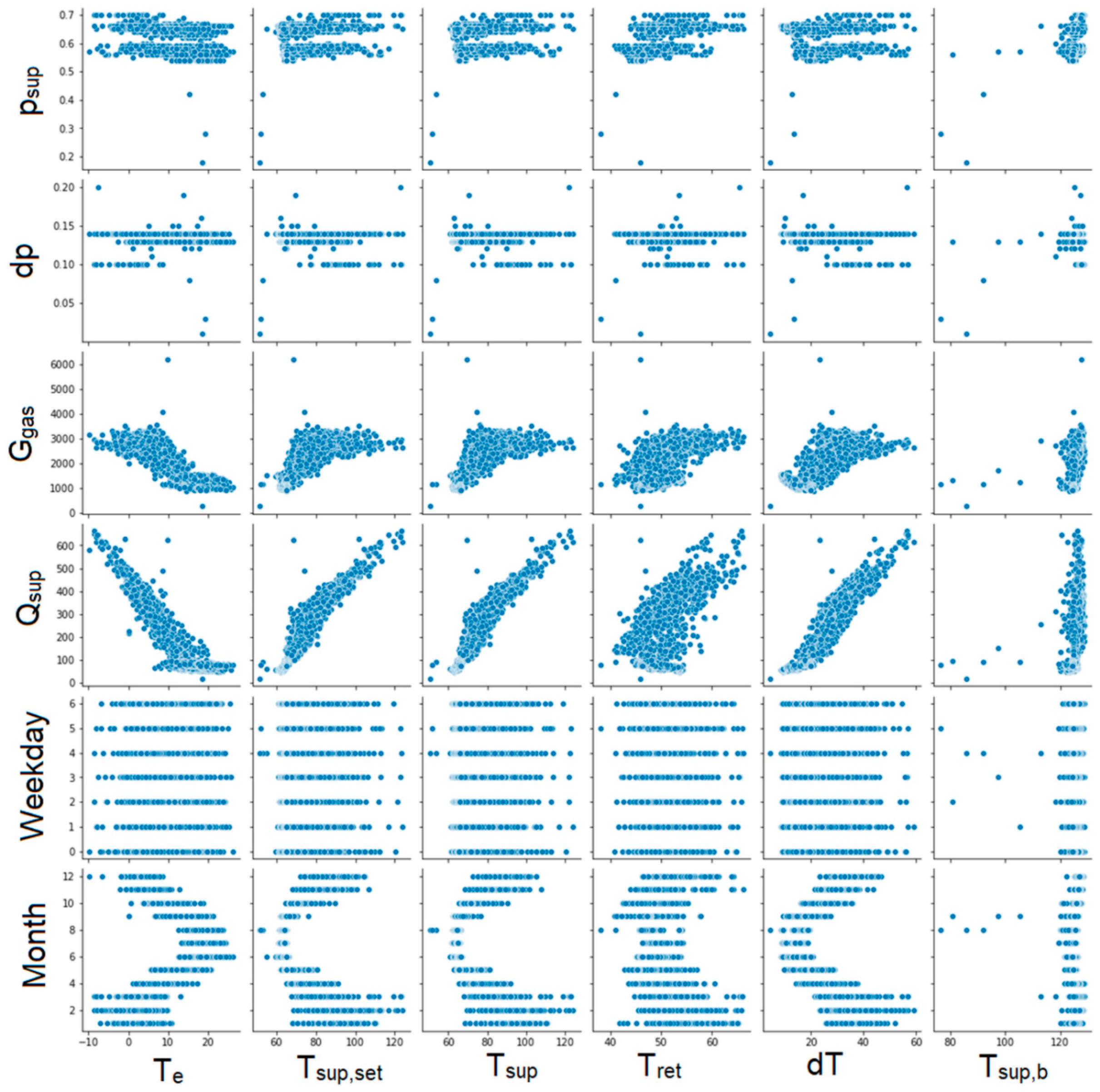
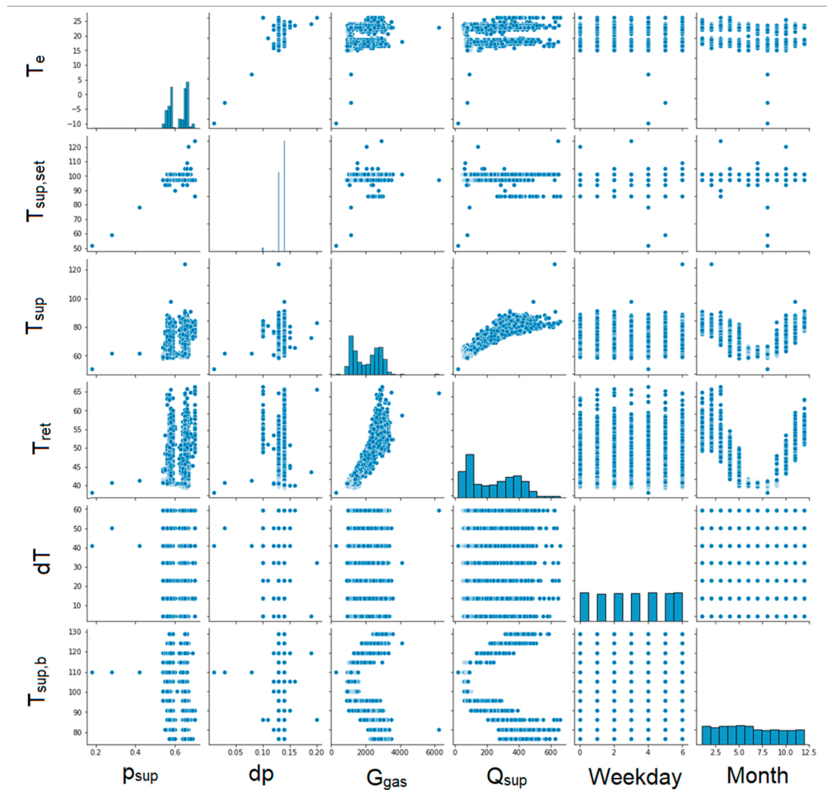
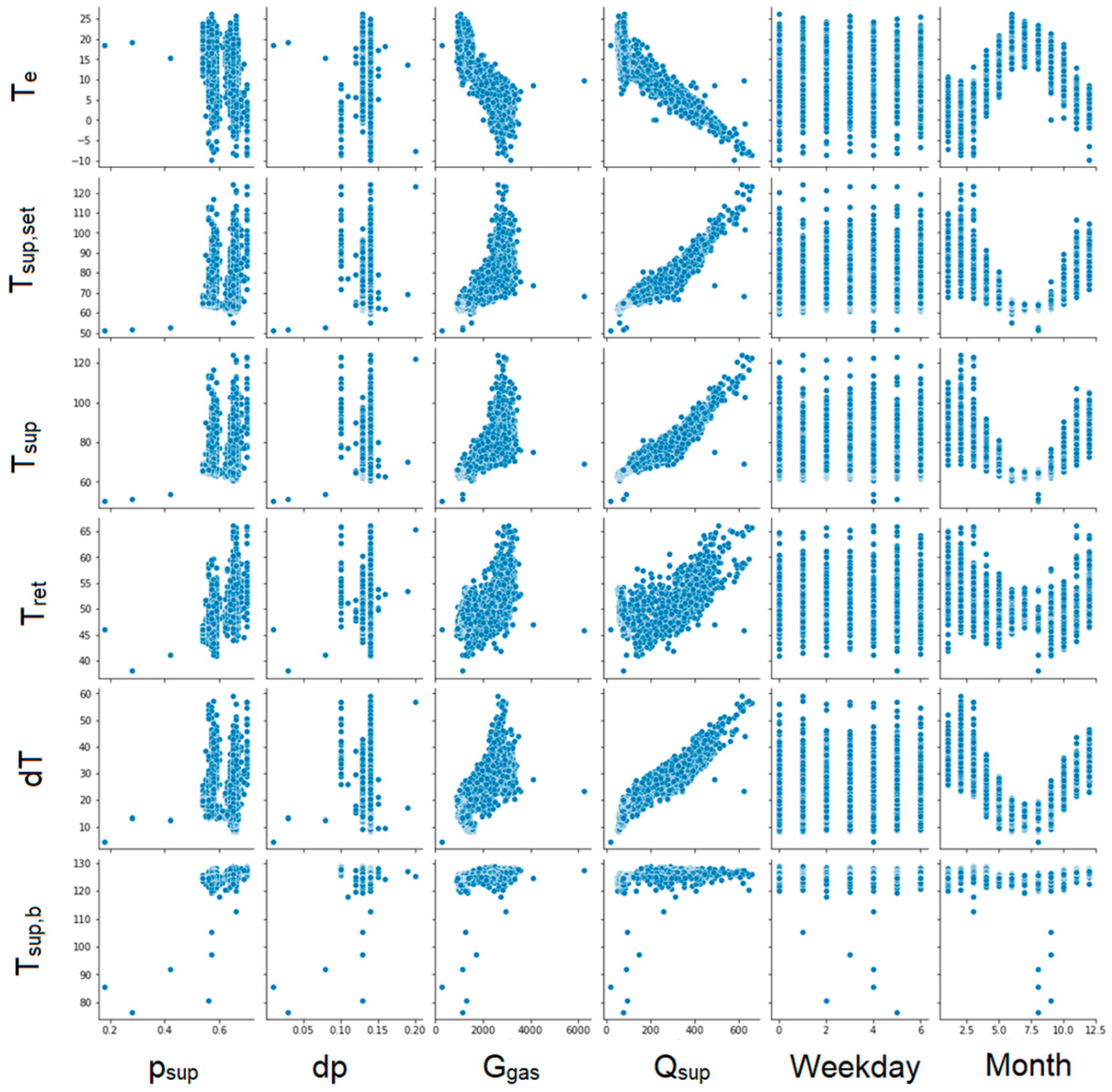
The next step was to create graphs for each pair of parameters to illustrate the correlation between them (Figure 6, Figure 7, Figure 8 and Figure 9). Unfortunately, some of the graphs show that some data are redundant. For example, as the supplying and return temperatures were available, there was no need to use their difference.
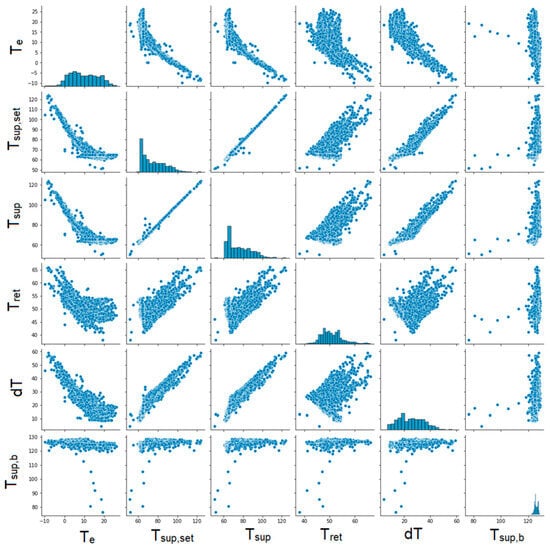
Figure 6.
Graphs showing correlations between individual parameters. Part 1.

Figure 7.
Graphs showing correlations between individual parameters. Part 2.
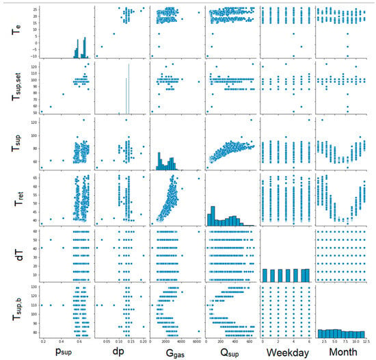
Figure 8.
Graphs showing correlations between individual parameters. Part 3.
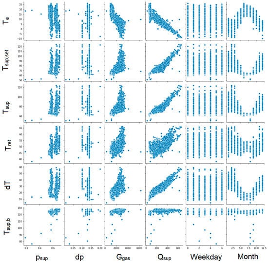
Figure 9.
Graphs showing correlations between individual parameters. Part 4.
3. Simulation Programme
3.1. Programming Environment
The data analysis as well as the entire process of creating the neural network was carried out using the Python language, which is clear and versatile. The availability of numerous libraries, add-ons and modules, which enable simple work with data, makes this language commonly used in many industrial and scientific applications. As an open-source product, it is readily used on all available platforms, such as Windows, Linux and McOS. Python is a high-level language, which makes the programme code created concise, clear and, therefore, easy and understandable for the user.
3.2. Keras Library
Keras is a machine learning library for the Python language, first released in 2015. Keras offers consistent and simple APIs, minimises the number of user actions required for typical use cases and provides clear and useful error messages. It also includes extensive documentation and guides for developers. Keras can run on a variety of engines, such as Tensorflow, Theano, PlaidML, MXNet and CNTK. In the case of this study, the Tesorflow engine was used. As Keras is based on Tensorflow, it is fully GPU-compatible, which contributes significantly to speeding up model training on large training sets.
3.3. Simulation Algorithm
The programme developed consists of two files. The first one defines the computational model of the neural network and performs the training of the network based on the imported data; the result of running it is the file model.keras, which stores the exported network model. Then, to use the created model in practise, a file defining the user interface is written. Here, windows and functions are defined (Figure 10).

Figure 10.
Algorithm of source code operation.
3.4. Data Scaling
Due to the variety of input data, the different units used and the different order of stored values, it was necessary to scale the data so that the validity of any of the columns was not implied by the nature of the column value. To this end, column values were reduced to values in the range <–1,1>. For each column of values, the arithmetic mean and standard deviation were calculated. The value of the arithmetic mean was then subtracted from each value and the result was divided by the value of the standard deviation so that the values were brought into the desired range:
with
- Xstand—the standardised value;
- Xavg—the average value;
- σ—the standard deviation.
To avoid the influence of the test set on the value of the arithmetic mean and standard deviation, these were calculated using the training set and were then used to scale part of the test data.
The scaled data were fitted for further analysis. Scaling can take various forms, and in some cases, more complex methods are required, e.g., when dealing with graphics files, it is necessary to convert graphics into a sequence of numerical values.
An additional way to adapt the data to the computational needs is normalisation, which involves reducing the range of data to values in the interval <0; 1>:
with
- Xnorm—the normalised value;
- Xmin—the minimum value;
- Xmax—the maximum value.
This method can be used when the data are subject to a normal distribution. In other cases, standardisation works well.
3.5. Model of the Neural Network
Among a vast variety of possible architectures of neural networks, the authors decided to use a DNN (deep neural network) in a quite simple architecture, which was FFN (feedforward neural network). This kind of neural network allows for the regression, classification and processing of signals, such as time series, while requiring low hardware requirements. This is achieved because of several simplifications of the network design: the data flow is unidirectional, there are no loops or feedback, and the data do not return to previous layers. At the same time, such networks (FNNs) can have a multilayer structure, allowing for deeper representation, good generalisation and error reduction, flexibility in modelling, good error reduction and relatively high optimisation capabilities.
Due to the fact of having a low number of input data records (~1500), there is a high probability of the network’s overfitting during the learning process. Building a small network is one way to minimise the occurrence of this phenomenon. To choose the right solution, we performed a literature review on similar solutions (Table 5).

Table 5.
Parameters of neural networks used in energy consumption forecasts.
Based on it, we developed a network with two hidden layers. It was created using the Sequential class from the Keras library, which means that layers are added sequentially one by one (Figure 11).
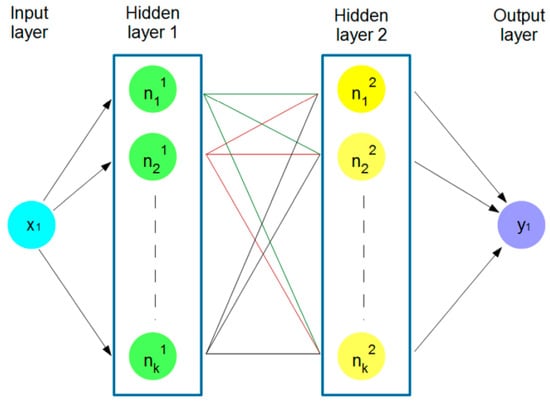
Figure 11.
Structure of the artificial network.
The layers added to the model are dense (dense) layers. The first and the second dense layers have 64 units (neurons, i.e., k = 64 in Figure 11) and use the Rectified Linear Unit (ReLu) activation functions [45]. The last dense layer has 1 unit, suggesting that the model is intended for regression (predicting continuous values). In this layer, the activation function was not defined, which resulted in a full range of values at the output. If the sigmoid function was used, the values generated would be in the range 0–1, and it would require an additional transformation to a range appropriate for the forecasted parameter.
The model was compiled with the rmsprop optimiser. The loss function MSE (mean squared error) was used to optimise the written model and was minimised during the training. The metric MAE (mean absolute error) was used to assess the performance of the written model and the output from this function was not used when training the model.
3.6. Algorithm for k-Component Cross-Validation
The k-component validation algorithm was used to divide the entire dataset into smaller parts and then to use one of them to validate the learning process. The algorithm was executed so many times that each part, which by default was a training set, at some point became a validation set. The use of this type of algorithm minimised the error resulting from the random selection of a validation set. Figure 12 shows the data partitioning scheme used in the network learning process for k = 4.

Figure 12.
Flow chart of the k-method—cross-validation.
3.7. User Interface
In order to use the neural network model in an easy and intuitive way, it is necessary to prepare an interface intended for the users, i.e., the process engineers of the district heating plant. To this end, the PyQt5 module dedicated to GUI windows design was used. A tool for creating and editing windows, PyQt5 Designer, is available with the PyQt5 library. It is a very intuitive editor that significantly speeds up the programmer’s work. The editor offers an intuitive interface with many basic options for selecting common elements such as buttons, windows, checkboxes or labels. It is possible to create a new window and then use the drag-and-drop method to add the desired elements. Once the final visualisation of the window has been created, it is possible to save a file with the extension .ui, which then needs to be converted to a file with the extension .py to configure and adjust the logic behind the functions and individual elements.
The algorithm of this part of the developed tool is presented in Figure 13. After importing the developed model to Keras, the programme’s main window presents a welcome message and information about the measurement data used to create the neural network model. When the button is clicked, an auxiliary window is launched with a request for the forecast ambient temperature for the day indicated by the user. After entering the value and confirming it with the ‘OK’ button, a function is started and the value of heat demand based on the entered temperature is computed. The calculation requires a neural network model created as a result of running the master file. The forecast value is presented in the message of the main window.

Figure 13.
Algorithm of forecast tool operation.
4. Results and Discussion
Network Performance
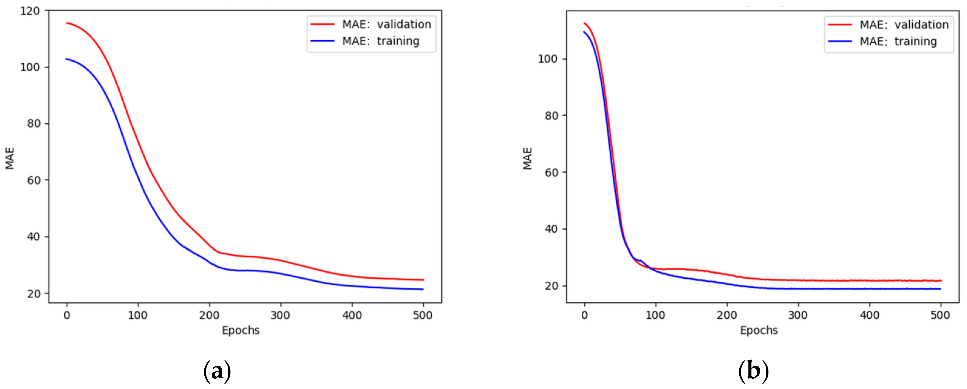
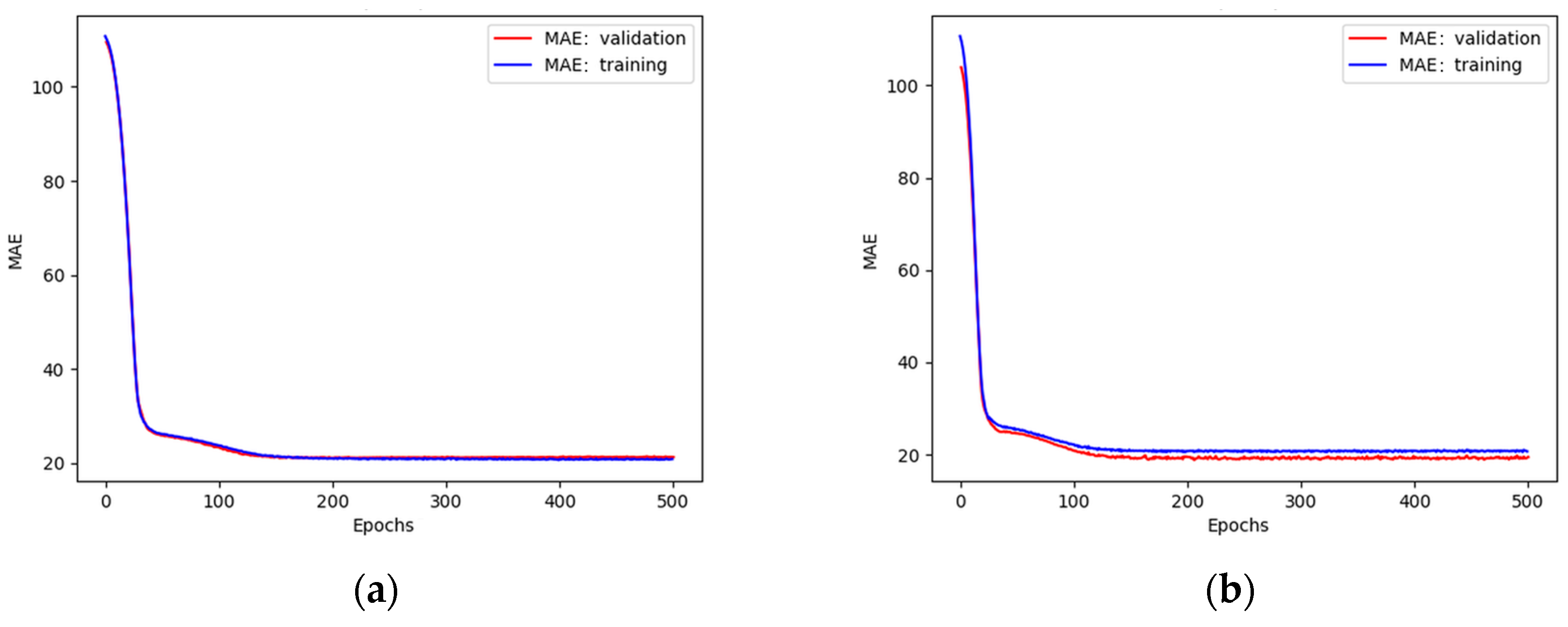
As mentioned previously, a cross-validation process for k = 4 was used. The input dataset was divided into 20% and 80% of test and train subsets, respectively. Before the necessary number of neurons was set, several tests were performed at first. The maximum number of 500 epochs was set and the MAE was plotted (Figure 14 and Figure 15) for different numbers of neurons.
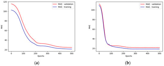
Figure 14.
Plots of MAE against the number of epochs during training and validation of a network with (a) 8 neurons in each layer; (b) 32 neurons in each layer.
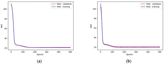
Figure 15.
Plots of MAE against the number of epochs during training and validation of a network with (a) 64 neurons in each layer; (b) 120 neurons in each layer.
The plots presented in Figure 14 show that validation curves are higher than training curves, which means that the model tends to overfit [46] when using 8 and 32 neurons in each layer. This problem was solved by increasing the number of neurons (Figure 15).
The satisfactory quality of the model was obtained for 64 neurons. A further increase in their number led to underfit behaviour.
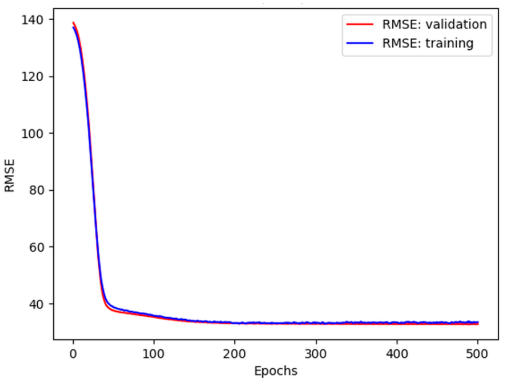
A good fit trend between the training and validation curves in Figure 15a was obtained when the number of epochs was above 150. Further learning beyond this value did not contribute to a reduction in error or the reduction in error was imperceptible. This conclusion is consistent with [47] and can be seen in Figure 16.
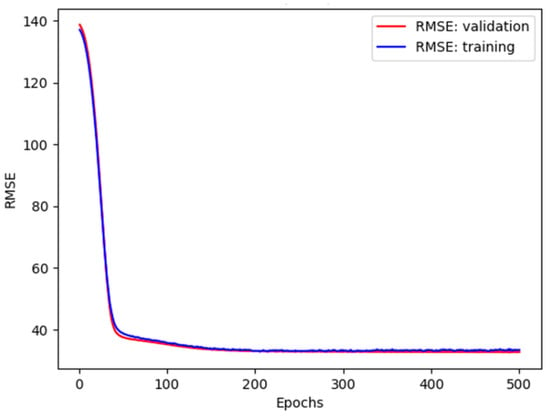
Figure 16.
The RMSE training and validation errors for the 64 neurons.
To obtain the final result, a final model was run on the previously prepared test data and fed into the test set to test the effectiveness of the training. The resulting mean average percentage error (MAPE) was 15%. Various measures assess the effectiveness of neural networks [48,49,50]. However, MAPE is probably the most commonly used in the evaluation of the accuracy of ANN predictions (Table 6).

Table 6.
Accuracy metrics in various data-driven forecast methods of DHSs.
Wojdyga [51] tested four different neural networks. In the first test case, the author compared one-hour-, two-hour- and three-hour-ahead forecasts using the same training dataset. The MAPE was 2.9%, 4.1% and 4.7%, respectively. In the second case, one-hour-ahead prediction was based on heat load data from one day and two days before, resulting in MAPEs of 2.1% and 4.2%, respectively.
Chramcov and Vařacha [18] used the outdoor temperature and time of the day (social component) as the main driving factors to produce a heat load forecast. Neural Network Synthesis was applied and half-hourly heat demand data were used. They obtained an MAPE average value of 5–6% and 8.5% with and without the inclusion of outdoor temperature in the input dataset.
The next step was to compare the performance of the developed ANN model with regression models. Based on the data presented in Figure 2, there were five derived heating curves, as given in Table 7.

Table 7.
Regression models of heating energy.
In this study, the test data that were not used in the training and validation process were entered in the developed model. The average relative error for n samples was then computed:
Then, prediction effectiveness was obtained from the following relationship:
In the considered case, EP = 0.850 for the ANN model.
Increasing the degree of the polynomial from 2 to 3 was more effective than from 3 to 4. In the latter case, there was no improvement in forecast accuracy. The lowest R2 coefficient was 0.855 in the case of the exponential model, which means that over 92% of the variance in heating energy was explained by the independent variable (external temperature) in the model. This indicates a very strong correlation [52]. Nevertheless, prediction effectiveness in all cases was lower than that of the solution based on the neural network. Hence, the proposed model is the most effective.
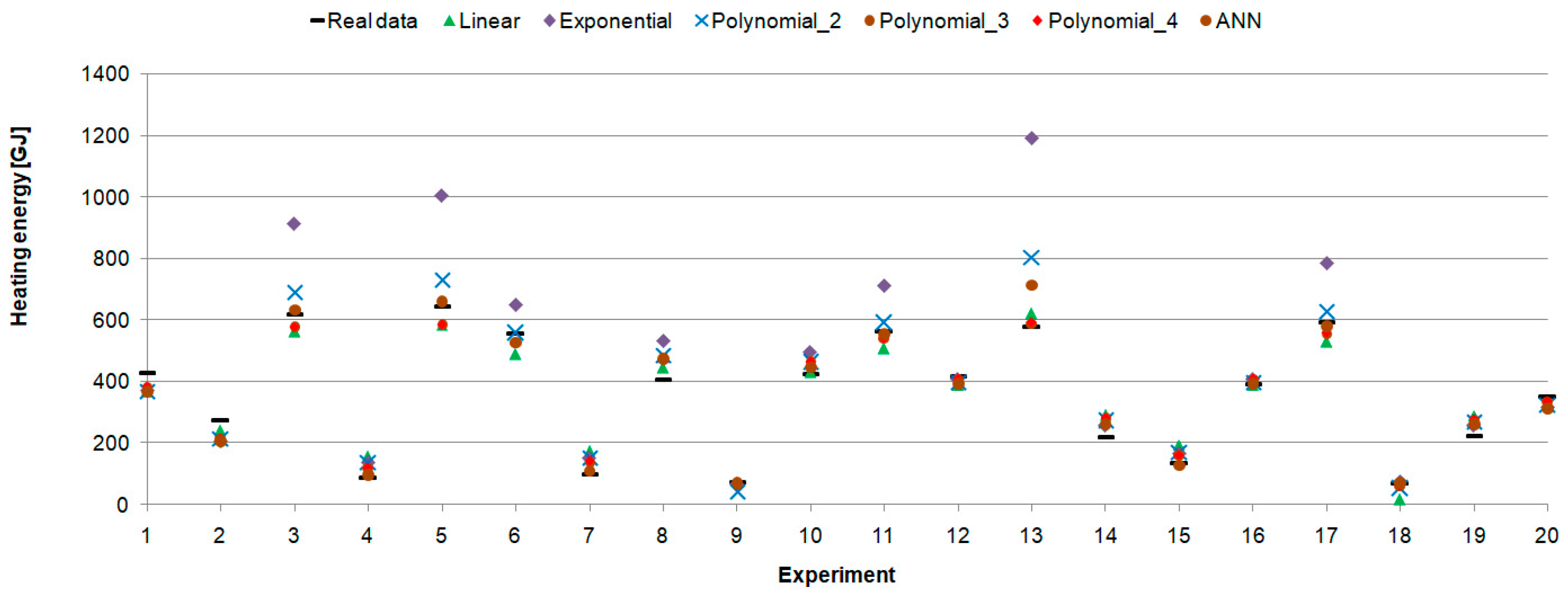
These results were confirmed in the experiment using 20 randomly selected test data points for which heating demand was estimated by all presented models (Figure 17). It showed good accuracy of the presented model and its ability to effectively predict daily heating production.
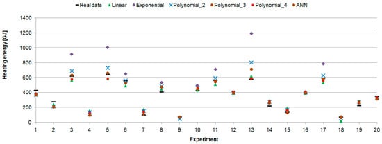
Figure 17.
Real and predicted heating energy.
Currently, boilers in the plant are controlled using a heating curve that links output thermal power (heating water flow rate, supply and return temperatures) with ambient temperature.
5. Conclusions
The main research objective of this study was to develop an efficient heat demand forecasting model using a neural network. The simple model of an ANN with two hidden layers was written in Python and built using freely available software. As it is commonly available among the variables measured in heating plants, the ambient air temperature was used as the input parameter to this model. The accuracy of the prediction assessed by mean absolute percentage error, MAPE = 15%, was at a level comparable with several studies. Some authors reported better results. However, they focused on hourly forecasts using hourly weather data. In this study, only a limited amount of daily input data were available. Therefore, it can be concluded that the developed model performed properly.
In the next step, using the same input data, four heating curves were developed and then used in the heat demand forecast. To compare their effects with the new model, there was a new indicator proposed: prediction effectiveness. The presented results showed that the ANN model performed the best.
The conclusions confirm that neural networks are promising tools in the field of artificial intelligence. However, to fully exploit their potential, further research and development of the technology are needed, especially in the context of heat demand forecasting.
In further steps, it would be advisable to develop the presented topic in two ways. The first one includes the measurement of new meteorological parameters influencing heating demand, such as solar irradiance or wind speed. The second one is to perform hourly measurements instead of current measurements with daily resolution. Then, a new, more accurate forecast model could be developed and practically used.
Author Contributions
Conceptualization, A.M. and P.M.; methodology, A.M. and P.M.; software (Python 3.10), A.M.; validation, A.M.; formal analysis, M.B.; investigation, A.M. and J.S.; resources, P.M.; data curation, J.S.; writing—original draft preparation, P.M.; writing—review and editing, P.M., J.S. and M.B.; visualisation, A.M.; supervision, P.M.; project administration, M.B.; funding acquisition, M.B. All authors have read and agreed to the published version of the manuscript.
Funding
This research received no external funding.
Data Availability Statement
The input data are confidential.
Conflicts of Interest
The authors declare no conflicts of interest.
Symbols and Abbreviations
| date | day and month of a year; hour of a day |
| day | day of a week |
| holiday | distinction between working day and holiday |
| EE | electrical energy |
| HL | heating load |
| Isol | solar irradiance |
| pret | return water pressure |
| psup | supply water pressure |
| qwater | heating water flow rate |
| RH | relative humidity of ambient air |
| SF | sunlight factor |
| Ti | indoor air temperature in a building |
| Te | external air temperature |
| Tret | return water temperature |
| Tsup | supply water temperature |
| Vwind | wind velocity |
| σ | standard deviation |
| Ac-GRN | Active Graph Recurrent Network |
| ANFIS | adaptive neuro-fuzzy inference system |
| BP | back propagation |
| BiLSTM | Bidirectional Long Short-Term Memory network |
| DWT | discrete wavelet transform |
| ETR | extremely randomised tree regression |
| GAM | Generalised Additive Model |
| GBDT | gradient boosting decision tree |
| MLP | Multilayer Perceptron |
| MLR | Multivariate linear regression |
| NARX | nonlinear autoregressive neural network model with external inputs |
| OLS | Ordinary Least Squares Regression |
| SLFN | single-layer feedforward neural network |
| SOMA | Self-Organising Migration Algorithm |
| SVR | Support Vector Regression |
| TCN | Temporal Convolutional Network |
References
- Energy 2023. Central Statistical Office. Rzeszów 2023. Available online: https://stat.gov.pl/en/topics/environment-energy/energy/energy-2023,1,11.html (accessed on 11 June 2024).
- Housing Economy and Municipal Infrastructure in 2022. Statistics Poland. Statistical Office in Lublin, Warsaw, Lublin 2023. Available online: https://stat.gov.pl/en/topics/municipal-infrastructure/municipal-infrastructure/housing-economy-and-municipal-infrastructure-in-2022,5,19.html (accessed on 11 June 2024).
- Municipal infrastructure—Energy and Gas Supply System in 2022. Statistics Poland. News Releases. 14 September 2023. Available online: https://stat.gov.pl/en/topics/municipal-infrastructure/municipal-infrastructure/municipal-infrastructure-energy-and-gas-supply-system-in-2022,12,1.html (accessed on 11 June 2024).
- Li, Q.; Jiang, S.; Wu, X. The Elman Network of Heat Load Forecast Based on the Temperature and Sunlight Factor. In Advancements in Smart City and Intelligent Building. ICSCIB 2018; Fang, Q., Zhu, Q., Qiao, F., Eds.; Advances in Intelligent Systems and Computing; Springer: Singapore, 2019; Volume 890. [Google Scholar] [CrossRef]
- Gadd, H.; Werner, S. Daily heat load variations in Swedish district heating systems. Appl. Energy 2013, 106, 47–55. [Google Scholar] [CrossRef]
- Gong, M.; Wang, J.; Bai, Y.; Li, B.; Zhang, L. Heat load prediction of residential buildings based on discrete wavelet transform and tree-based ensemble learning. J. Build. Eng. 2020, 32, 101455. [Google Scholar] [CrossRef]
- Wang, C.; Li, X.; Li, H. Role of input features in developing data-driven models for building thermal demand forecast. Energy Build. 2022, 277, 112593. [Google Scholar] [CrossRef]
- Wang, Y.; Li, Z.; Liu, J.; Zhao, Y.; Sun, S. A novel combined model for heat load prediction in district heating systems. Appl. Therm. Eng. 2023, 227, 120372. [Google Scholar] [CrossRef]
- Huang, Y.; Zhao, Y.; Wang, Z.; Liu, X.; Liu, H.; Fu, Y. Explainable district heat load forecasting with active deep learning. Appl. Energy 2023, 350, 121753. [Google Scholar] [CrossRef]
- Oyucu, S.; Dogan, F.; Aksöz, A.; Biçer, E. Comparative Analysis of Commonly Used Machine Learning Approaches for Li-Ion Battery Performance Prediction and Management in Electric Vehicles. Appl. Sci. 2024, 14, 2306. [Google Scholar] [CrossRef]
- Ma, W.; Fang, S.; Liu, G.; Zhou, R. Modeling of district load forecasting for distributed energy system. Appl. Energy 2017, 204, 181–205. [Google Scholar] [CrossRef]
- Mosavi, A.; Salimi, M.; Faizollahzadeh Ardabili, S.; Rabczuk, T.; Shamshirband, S.; Varkonyi-Koczy, A.R. State of the Art of Machine Learning Models in Energy Systems, a Systematic Review. Energies 2019, 12, 1301. [Google Scholar] [CrossRef]
- Livingstone, D.; Manallack, D.; Tetko, I. Data modelling with neural networks: Advantages and limitations. J. Comput. Aided Mol. Des. 1997, 11, 135–142. [Google Scholar] [CrossRef]
- Hua, P.; Wang, H.; Xie, Z.; Lahdelma, R. District heating load patterns and short-term forecasting for buildings and city level. Energy 2024, 289, 129866. [Google Scholar] [CrossRef]
- Forootan, M.M.; Larki, I.; Zahedi, R.; Ahmadi, A. Machine Learning and Deep Learning in Energy Systems: A Review. Sustainability 2022, 14, 4832. [Google Scholar] [CrossRef]
- Simonović, M.B.; Nikolić, V.D.; Petrović, E.P.; Ćirić, I.T. Heat load prediction of small district heating system using artificial neural networks. Therm. Sci. 2017, 21, 1355–1365. [Google Scholar] [CrossRef]
- Gong, M.; Zhou, H.; Wang, Q.; Wang, S.; Yang, P. District heating systems load forecasting: A deep neural networks model based on similar day approach. Adv. Build. Energy Res. 2019, 14, 372–388. [Google Scholar] [CrossRef]
- Chramcov, B.; Vařacha, P. Usage of the Evolutionary Designed Neural Network for Heat Demand Forecast. In Nostradamus: Modern Methods of Prediction, Modeling and Analysis of Nonlinear Systems; Zelinka, I., Rössler, O., Snášel, V., Abraham, A., Corchado, E., Eds.; Advances in Intelligent Systems and Computing; Springer: Berlin/Heidelberg, Germany, 2013; Volume 192. [Google Scholar] [CrossRef]
- Bujalski, M.; Madejski, P.; Fuzowski, K. Day-ahead heat load forecasting during the off-season in the district heating system using Generalized Additive model. Energy Build. 2023, 278, 112630. [Google Scholar] [CrossRef]
- Abghari, S.; Garcia-Martin, E.; Johansson, C.; Lavesson, N.; Grahn, H. Trend Analysis to Automatically Identify Heat Program Changes. Energy Procedia 2017, 116, 407–415. [Google Scholar] [CrossRef]
- Żymełka, P.Y.; Szega, M. Short-term scheduling of gas-fired CHP plant with thermal storage using optimization algorithm and forecasting models. Energy Convers. Manag. 2021, 231, 113860. [Google Scholar] [CrossRef]
- Petković, D.; Protić, M.; Shamshirband, S.; Akib, S.; Raos, M.; Marković, D. Evaluation of the most influential parameters of heat load in district heating systems. Energy Build. 2015, 104, 264–274. [Google Scholar] [CrossRef]
- Suryanarayana, G.; Lago, J.; Geysen, D.; Aleksiejuk, P.; Johansson, C. Thermal load forecasting in district heating networks using deep learning and advanced feature selection methods. Energy 2018, 157, 141–149. [Google Scholar] [CrossRef]
- Kováč, S.; Micha’čonok, G.; Halenár, I.; Važan, P. Comparison of Heat Demand Prediction Using Wavelet Analysis and Neural Network for a District Heating Network. Energies 2021, 14, 1545. [Google Scholar] [CrossRef]
- Song, J.; Li, W.; Zhu, S.; Zhou, C.; Xue, G.; Wu, X. Predicting hourly heating load in district heating system based on the hybrid Bi-directional long short-term memory and temporal convolutional network model. J. Clean. Prod. 2024, 463, 142769. [Google Scholar] [CrossRef]
- An, W.; Zhu, X.; Yang, K.; Kim, M.K.; Liu, J. Hourly Heat Load Prediction for Residential Buildings Based on Multiple Combination Models: A Comparative Study. Buildings 2023, 13, 2340. [Google Scholar] [CrossRef]
- Hietaharju, P.; Ruusunen, M.; Leiviskä, K. Enabling Demand Side Management: Heat Demand Forecasting at City Level. Materials 2019, 12, 202. [Google Scholar] [CrossRef] [PubMed]
- Manno, A.; Martelli, E.; Amaldi, E. A Shallow Neural Network Approach for the Short-Term Forecast of Hourly Energy Consumption. Energies 2022, 15, 958. [Google Scholar] [CrossRef]
- Dahl, M.; Brun, A.; Kirsebom, O.S.; Andresen, G.B. Improving Short-Term Heat Load Forecasts with Calendar and Holiday Data. Energies 2018, 11, 1678. [Google Scholar] [CrossRef]
- Idowu, S.; Saguna, S.; Ahlund, C.; Schelen, O. Applied machine learning: Forecasting heat load in district heating system. Energy Build. 2016, 133, 478–488. [Google Scholar] [CrossRef]
- Li, B.; Shao, Y.; Lian, Y.; Li, P.; Lei, Q. Bayesian Optimization-Based LSTM for Short-Term Heating Load Forecasting. Energies 2023, 16, 6234. [Google Scholar] [CrossRef]
- Wei, Z.; Zhang, T.; Yue, B.; Ding, Y.; Xiao, R.; Wang, R.; Zhai, X. Prediction of residential district heating load based on machine learning: A case study. Energy 2021, 231, 120950. [Google Scholar] [CrossRef]
- Bujalski, M.; Madejski, P.; Fuzowski, K. Heat demand forecasting in District Heating Network using XGBoost algorithm. E3S Web Conf. 2021, 323, 00004. [Google Scholar] [CrossRef]
- Bujalski, M.; Madejski, P. Forecasting of Heat Production in Combined Heat and Power Plants Using Generalized Additive Models. Energies 2021, 14, 2331. [Google Scholar] [CrossRef]
- Månsson, S.; Kallioniemi, P.-O.J.; Sernhed, K.; Thern, M. A machine learning approach to fault detection in district heating substations. Energy Procedia 2018, 149, 226–235. [Google Scholar] [CrossRef]
- Szymiczek, J.; Szczotka, K.; Banaś, M.; Jura, P. Efficiency of a Compressor Heat Pump System in Different Cycle Designs: A Simulation Study for Low-Enthalpy Geothermal Resources. Energies 2022, 15, 5546. [Google Scholar] [CrossRef]
- Stienecker, M.; Hagemeier, A. Developing Feedforward Neural Networks as Benchmark for Load Forecasting: Methodology Presentation and Application to Hospital Heat Load Forecasting. Energies 2023, 16, 2026. [Google Scholar] [CrossRef]
- Dagdougui, H.; Bagheri, F.; Le, H.; Dessaint, L. Neural Network Model for Short-Term and Very-Short-Term Load Forecasting in District Buildings. Energy Build. 2019, 203, 109408. [Google Scholar] [CrossRef]
- Wang, H.T. Typical Building Thermal and Thermal Load Forecasting Based on Wavelet Neural Network. Procedia Comput. Sci. 2020, 166, 529–533. [Google Scholar] [CrossRef]
- Trabert, U.; Pag, F.; Orozaliev, J.; Jordan, U.; Vajen, K. Peak shaving at system level with a large district heating substation using deep learning forecasting models. Energy 2024, 301, 131690. [Google Scholar] [CrossRef]
- Salehi, S.; Kavgic, M.; Bonakdari, H.; Begnoche, L. Comparative study of univariate and multivariate strategy for short-term forecasting of heat demand density: Exploring single and hybrid deep learning models. Energy AI 2024, 16, 100343. [Google Scholar] [CrossRef]
- Gao, Z.; Yu, J.; Zhao, A.; Hu, Q.; Yang, S. A hybrid method of cooling load forecasting for large commercial building based on extreme learning machine. Energy 2022, 238, 122073. [Google Scholar] [CrossRef]
- Semmelmann, L.; Hertel, M.; Kircher, K.J.; Mikut, R.; Hagenmeyer, V.; Weinhardt, C. The impact of heat pumps on day-ahead energy community load forecasting. Appl. Energy 2024, 368, 123364. [Google Scholar] [CrossRef]
- Shi, J.; Teh, J. Load forecasting for regional integrated energy system based on complementary ensemble empirical mode de-composition and multi-model fusion. Appl. Energy 2024, 353, 122146. [Google Scholar] [CrossRef]
- Wang, Y.; Li, Y.; Song, Y.; Rong, X. The Influence of the Activation Function in a Convolution Neural Network Model of Facial Expression Recognition. Appl. Sci. 2020, 10, 1897. [Google Scholar] [CrossRef]
- Candela-Leal, M.O.; Gutiérrez-Flores, E.A.; Presbítero-Espinosa, G.; Sujatha-Ravindran, A.; Ramírez-Mendoza, R.A.; Lozoya-Santos, J.d.J.; Ramírez-Moreno, M.A. Multi-Output Sequential Deep Learning Model for Athlete Force Prediction on a Treadmill Using 3D Markers. Appl. Sci. 2022, 12, 5424. [Google Scholar] [CrossRef]
- Salah, S.; Alsamamra, H.R.; Shoqeir, J.H. Exploring Wind Speed for Energy Considerations in Eastern Jerusalem-Palestine Using Machine-Learning Algorithms. Energies 2022, 15, 2602. [Google Scholar] [CrossRef]
- Sokół, S.; Pawuś, D.; Majewski, P.; Krok, M. The Study of the Effectiveness of Advanced Algorithms for Learning Neural Networks Based on FPGA in the Musical Notation Classification Task. Appl. Sci. 2022, 12, 9829. [Google Scholar] [CrossRef]
- Stokfiszewski, K.; Sztoch, P.; Sztoch, R.; Wosiak, A. Building Energy Use Intensity Prediction with Artificial Neural Networks. In Progress in Polish Artificial Intelligence Research 4; Wojciechowski, A., Lipiński, P., Eds.; Monografie Politechniki Łódzkiej Nr. 2437; Wydawnictwo Politechniki Łódzkiej: Łódź, Poland, 2023; pp. 313–318. [Google Scholar] [CrossRef]
- Karunia, K.; Putri, A.E.; Fachriani, M.D.; Rois, M.H. Evaluation of the Effectiveness of Neural Network Models for Analyzing Customer Review Sentiments on Marketplace. Public Res. J. Eng. Data Technol. Comput. Sci. 2024, 2, 52–59. [Google Scholar] [CrossRef]
- Wojdyga, K. Predicting Heat Demand for a District Heating Systems. Int. J. Energy Power Eng. 2014, 3, 237–244. [Google Scholar] [CrossRef]
- Jierula, A.; Wang, S.; OH, T.-M.; Wang, P. Study on Accuracy Metrics for Evaluating the Predictions of Damage Locations in Deep Piles Using Artificial Neural Networks with Acoustic Emission Data. Appl. Sci. 2021, 11, 2314. [Google Scholar] [CrossRef]
Disclaimer/Publisher’s Note: The statements, opinions and data contained in all publications are solely those of the individual author(s) and contributor(s) and not of MDPI and/or the editor(s). MDPI and/or the editor(s) disclaim responsibility for any injury to people or property resulting from any ideas, methods, instructions or products referred to in the content. |
© 2024 by the authors. Licensee MDPI, Basel, Switzerland. This article is an open access article distributed under the terms and conditions of the Creative Commons Attribution (CC BY) license (https://creativecommons.org/licenses/by/4.0/).

