Abstract
Forecasting the electricity market, even in the short term, is a difficult task, due to the nature of this commodity, the lack of storage capacity, and the multiplicity and volatility of factors that influence its price. The sensitivity of the market results in the appearance of anomalies in the market, during which forecasting models often break down. The aim of this paper is to present the possibility of using hybrid machine learning models to forecast the price of electricity, especially when such events occur. It includes the automatic detection of anomalies using three different switch types and two independent forecasting models, one for use during periods of stable markets and the other during periods of anomalies. The results of empirical tests conducted on data from the Polish energy market showed that the proposed solution improves the overall quality of prediction compared to using each model separately and significantly improves the quality of prediction during anomaly periods.
1. Introduction
Electricity is a commodity used in every area of human activity. As a result, electricity price forecasting (EPF) is extremely important and, given the nature of the commodity, difficult. Electricity prices are characterized by seasonality at various frequencies, high volatility, abnormal values, and sudden jumps in value, which is a direct result of the nature of the commodity. Regular price fluctuations are the result of cyclical changes in electricity demand, which is significantly higher during daytime peak hours and on weekdays compared to demand during night time hours or holidays. The high volatility as well as the unexpected appearance of abnormal values is mainly related to changing market conditions determined by economic, political, and technical factors in addition to the weather and the limited storage capacity of the commodity [1,2,3,4].
Due to the complexity of the problem, many works address the topic of EPF [4,5,6,7,8], and there are many approaches to EPF. They can be divided into two classes. The first involves econometric modeling and the second includes machine learning (ML) methods. Within the first approach, the literature includes works on the use of linear ARIMA models [9], nonlinear GARCH models [10,11] or taking into account price spikes [4,12]. Due to many factors potentially influencing the level of electricity prices, multiple parameters are included in univariate or multivariate econometric models [13,14]. However, when the number of parameters becomes too high this may cause overfitting. Another disadvantage of econometric methods is their predetermined error distribution, which may lead to model misspecification.
Due to the limitations of parametric econometric methods, ML methods are being used in parallel to forecast prices in the day-ahead markets. The authors of [6,15] obtained percentage errors of forecasts lower than those obtained with machine learning methods. Slightly better results than those of classical forecasts were also reported in the work [16] based on neural networks. A broad overview of the forecasting methods used can be found in a number of studies, including [6,17,18,19].
For both econometric and ML models, the challenge is to account for outlier observations, which occur unpredictably and tend to take on values that deviate significantly from typical price levels. However, they appear frequently enough in the time series of electricity prices that they cannot be neglected in the analysis and prediction. The problem of including periods of anomalies (sudden changes in the value of the price, spikes, jumps) has been known to researchers for a long time, and there have been numerous attempts to take them into account in price forecasting [20]. The fundamental motivation for undertaking this research was the observation that models that give good forecasts most of the time perform significantly worse during periods of anomaly. These errors are difficult to remove by systematically improving the model itself when these periods occur unpredictably and are relatively infrequent and short. Nonetheless, it is expected that the price of energy can be predicted well during such periods as well.
There are a few approaches to deal with the problem of spikes (anomalies). If abnormal values are identified in the time series, then they can be replaced by another value, such as the average of a similar day, or left unchanged. In the first case, we will get a model that predicts the value well in stable periods. In the second case, the model can reflect the abnormal conditions over the entire study period [4]. Regardless of the approach to identifying abnormal values, it is quite a challenge to predict such events from historical data. Also in [4], the author used a jump-diffusion model in which, in addition to drift and variability, a homogeneous Poisson process was used to represent the spikes. In contrast, in [21], a jump-diffusion model was based on a seasonal decomposition, with the Ornstein-Uhlenbeck component responsible for spikes driven by a Lévy process. A significant drawback of these approaches is the assumption of a fixed distribution of anomalies occurring in the future.
Forecasting that takes into account the occurrence of price spikes in the future can also be carried out using threshold autoregressive models [22] or Markov regime-switching models [23,24]. They rely on the division of periods into stable and unstable regimes. In threshold autoregressive models, one of two autoregressive models is selected depending on whether the indicated value exceeds a certain threshold. In Markov regime-switching models, different models are used for different price ranges. Which model is used is determined by the probability of the price falling into the specified range. The result obtained in [25] show that if spikes are identified in time series, these models are preferable to autoregressive models. There are also few proposals in the literature to adapt the idea of switches in hybrid ML models to forecasting in the energy market. In [26], Bayesian clustering by dynamics (BCD) is used along with support vector regression (SVR). The BCD procedure plays the role of a switch that classifies time series into clusters of similar variability characteristics. For every cluster, forecasts are obtained by independently fitting SVR models.
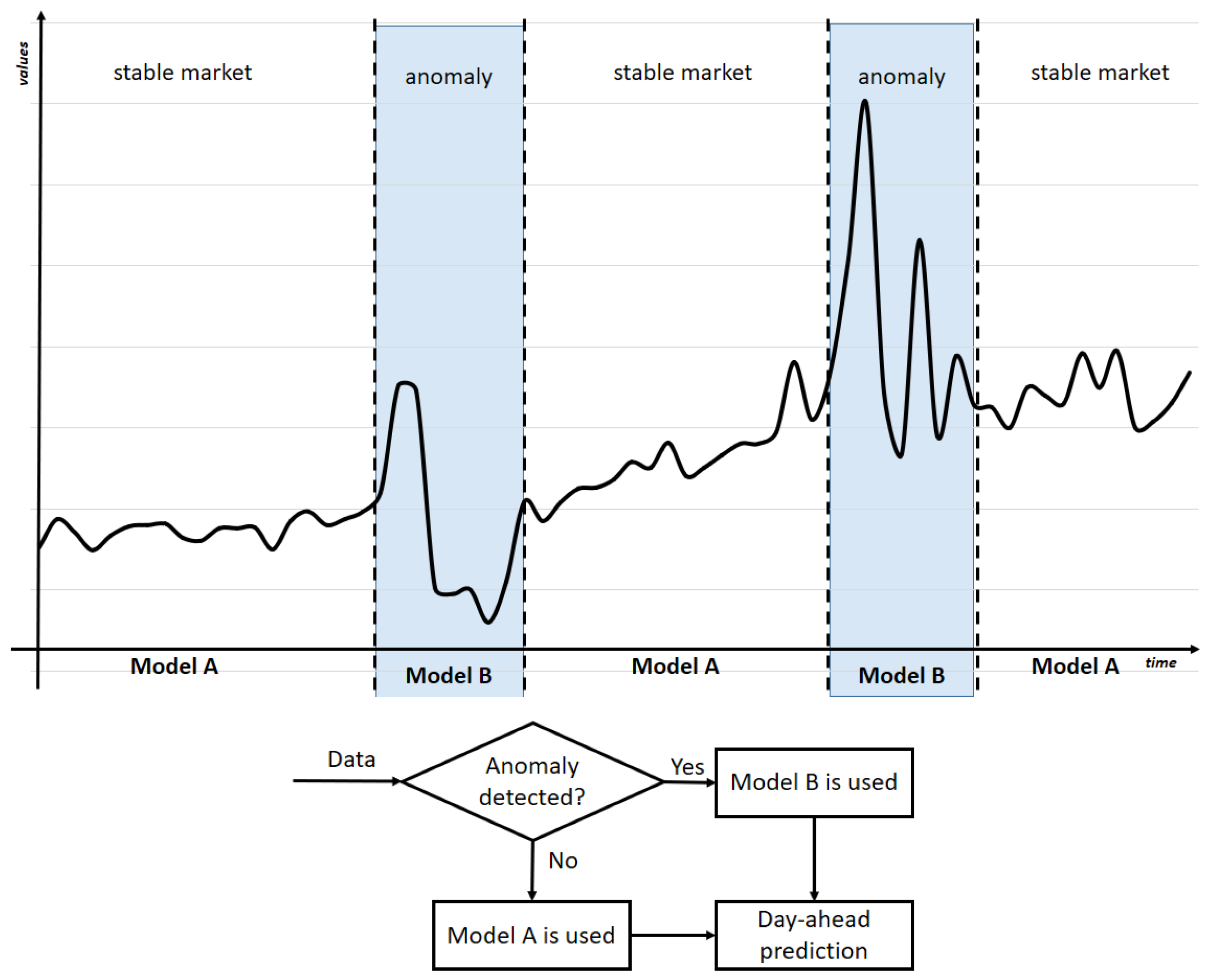
The solution proposed in this article uses the idea of threshold autoregressive models, but applies it to ML models. For three different threshold functions that distinguish between anomalous and stable periods, two independent predictive models based on a machine learning approach were proposed and combined into one hybrid model. During periods when the market is relatively stable, one model performs well, while during periods of anomalies, the other model is better. A key role in the performance of a procedure built this way is played by the model selection switch. A general sketch of our idea is shown in Figure 1.
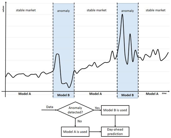
Figure 1.
General schema of the proposition.
The idea of forecasting energy prices using hybrid ML (HM) models has been presented in many articles, but to the best of our knowledge, our proposal is new due to the use of a switch model to divide the series into periods of stability and those that can be described as anomalies. The study aims to answer the question of whether such a predictive model will produce better overall results than any of its components individually. The purpose of this article is therefore to present the results of a study aimed at improving the predictive ability of existing machine-learning HMs to better account for the occurrence of anomalies and incorporate them into day-ahead energy market price forecasting.
The rest of the article is organized as follows. The Section 2 presents the theoretical background of the problem, including the causes of anomalies in the energy market, and briefly discusses the applications of HMs in EPFs. Section 3 presents the data and justification for the choice of the prediction quality measure used in the series of experiments, which are described in detail in the Section 4. Section 5 discusses the results of the experiments. The Section 6 presents the conclusions, limitations, and future works.
2. Theoretical Background
From a data analysis point of view, it is a common practice to interpret electric energy price time series as realizations of a stochastic process. It is frequently assumed that this process is non-stationary and anti-persistent, and the parameters of its distributions vary by seasons, days of the week, and hours, also exhibiting various anomalies [4,17]. Reducing the impact of random events on prediction quality is of practical importance for energy market participants. The results of the research provide important information, enabling them to make better investment decisions and manage risks better. This leads to the improvement of prediction tools and to the development of new models that are more resilient to unpredictable events.
2.1. Anomalies on Electricity Market
Price spikes are an inherent feature of electricity markets, and they substantially impact EPFs. They are interpreted as outlier observations. According to [27]: “An outlier is an observation that deviates so much from other observations as to arouse suspicion that it was generated by a different mechanism”. In turn, in [4] price spikes are defined as “prices that surpass a specified threshold for a brief period of time, but it is difficult to gain any consensus on what that threshold or time interval should be”. A broad and in-depth discussion on detecting and dealing with outliers has been carried out in many publications, including, among others: [4,6,12,20,28,29,30,31]. There are many factors that affect energy prices and cause spikes, including [32,33,34,35]:
- Weather conditions. When the share of renewable energy sources (RES) in energy production increases, the weather becomes one of the most important factors influencing the price. Temperature, cloud cover, rain, or snowfall, the occurrence of extreme weather events such as storms or heat waves have a direct impact on the demand and supply of electricity. At the same time, weather conditions affect the performance of power plants, especially those using RES such as hydroelectric, wind, or photovoltaic plants.
- Failures and disasters in both generation and transmission infrastructure. These events have a strongly destabilizing effect on the market. Any deviation from the plan in this respect causes large fluctuations in the price of energy.
- The actions of market participants who, as a result of various circumstances, fearing a shortage in the market, try to secure their energy supply at all costs.
- Price spikes for energy raw materials. Oil, natural gas and coal are still important sources of energy, and their prices have a significant impact on the price of electricity. At the same time, their prices often fluctuate rapidly in response to the international situation.
- Changes in government regulation and policy. Decisions on energy prices, subsidies for renewables, tax policy, or carbon emissions affect the cost of energy production and the price that is formed on the exchange.
- Social and political events, media reports, and rapid changes in public sentiment. Events such as armed conflicts, protests, strikes, roadblocks, or political changes also affect the energy market. Political or social instability in energy-producing regions or places of high energy consumption can lead to unexpected and sudden changes in price.
- Natural disasters like floods, earthquakes, hurricanes, etc. that affect infrastructure or generate spikes in energy demand.
- Errors made by people who make decisions about energy production, transmission, or consumption.
- Additional local factors influencing price volatility in the Polish market include:
- A large annual temperature amplitude (from −20 °C to +30 °C) over a small area;
- Large differences in day length throughout the year (from 8 to 16 h);
- A variable-transitional climate, lack of constant winds, and a relatively small number of days of sunshine (66 days—about 1600 h per year) with high variability in their timing throughout the year and frequent weather changes;
- A low share of stable RES due to unfavorable hydrological and wind conditions;
- A very high share of fossil fuels (coal and lignite) makes the entire energy system inflexible. Even when the possibility of obtaining large amounts of energy from RES arises, it is not possible to limit power production below a certain level, which is determined by the technical conditions of the coal or lignite units;
- The location and geopolitical uncertainty due to the proximity of an aggressive country and the periodically emerging problems of raw material availability in 2022–2023;
- The simultaneous influence of so many factors and unpredictable events introduces elements of chaos and unpredictability into the energy price time series.
In studies, price spikes can be treated like any other observation, as outliers to be eliminated before further investigation, or they can be treated as the main focus of the study [36,37]. They may belong to one of three following categories [38]:
- An abnormally high/low price;
- An abnormal jump in price, in which the difference of prices (absolute or relative) between two periods is higher than a given threshold;
- A close to zero or negative price.
The first category of spikes is most often the subject of research. A separate issue is the value or trajectory of a spike and the probability that it will occur [39].
Different approaches to the treatment of outliers can be found in the literature. One of them includes methods that focus on improving data quality, in which outliers are treated as data that should be removed (see [40]) or modified [41], while the other approach treats the data as correct and as data that should be included in the predictive model. From the perspective of our research, only the second approach is suitable.
2.2. Hybrid Models in Electricity Prediction
Combining different models for use in a single analytical task is a long-standing technique [1,42,43,44]. HMs use more than one model in an attempt to make the most of the capabilities of each model. Various statistical methods and ML methods are combined in energy market price prediction. For example, in [45], the authors combined ARIMA methods with neural networks. In [46], an autoregressive model was used to predict the linear components of the price series, while ANNs together with an EMD model were used to predict the nonlinear components. In turn, in [47], neural networks and genetic algorithms were used.
In [48], the wind speed is accounted for in the prediction of energy production by using Variational Mode Decomposition with a Fruit Fly Optimization algorithm in which ARIMA models and Deep Belief Networks are applied to model individual subcomponents. A two-step process that uses an extreme machine learning method to determine the forecast and then a maximum likelihood method to estimate the noise variance is presented in [49]. A sophisticated model using SVR and the bidirectional LSTM (long short-term memory) neural network with an attention mechanism was proposed in [50]. In [42], the forecast of the electrical energy price was calculated as a weighted average of individual predictions obtained using the following models: autoregressive moving average (ARMA), neural network autoregressive (NAR), random forest (RF), support vector regression (SVR), and gradient boosting machine (GBM). The weights in the average reflected the quality of forecasts assessed for these individual models.
The authors of [51] presented a wide review of diverse approaches to combining individual models for the purpose of improving forecasts. They identified three main categories of models: parallel hybrid structure, series hybrid structure, and parallel–series hybrid structure.
Under the first approach, the forecast is calculated by aggregating the output of multiple individual models. This is the oldest approach that may be found among others in [52]. The second approach, which is currently popular, relies on decomposing the time series into components that are modeled separately, then adding up the resulting predictions. This may be found in [53,54], in which the authors used ARIMA models for the linear component and neural networks for the nonlinear components. In [54], the time series was decomposed into seasonal and random components using an EMD (Empirical Mode Decomposition) method. In [55], nonlinear variability was characterized by Taylor expansion. Recursive-EMD and long short-term memory were also used in [56]. Both approaches may also be combined, as in [57].
Our proposal belongs to the first category of models, i.e., parallel hybrid structures. The forecast is calculated as a linear combination of two random forest models with dynamically varying weights, depending on the switch.
3. Data and Error Metrics
3.1. Data Description and Pre-Processing
Historical electricity prices with hourly frequencies from the Polish Power System Operation (www.pse.pl, accessed on 20 January 2024) were used for the analysis. The hour of the day, the day of the week, and the month were used as explanatory variables. Due to the autocorrelation of prices and the pronounced weekly cyclicality, the average electricity price from the week before was also used. The relationship between total domestic demand (total load) and the production capacity of the generating units in the National Electricity System was accounted for in the modeling. Additionally, the production capacities of JGWa (active) and JGMa (stored) were included. The total power and power achieved from the chosen sources (like wind and photovoltaic units) and the generation capacity that operates outside the Balancing Market were also used for modeling. The model also includes information about the power surpluses/shortages balance related to the exchange of electricity between countries. The information about power reserves above and below demand is also included (Table 1).

Table 1.
Variables included in the models.
Activity level is an additional variable introduced into the model to reflect overall activity in the country, taking into account calendar constraints like national holidays and days off that affect the natural weekly cycle of energy demand. “Forecast variable” is the average price of electricity sales RCEt in the competitive market (i.e., to trading companies under bilateral contracts and to the power exchange) in every hour in day-ahead market.
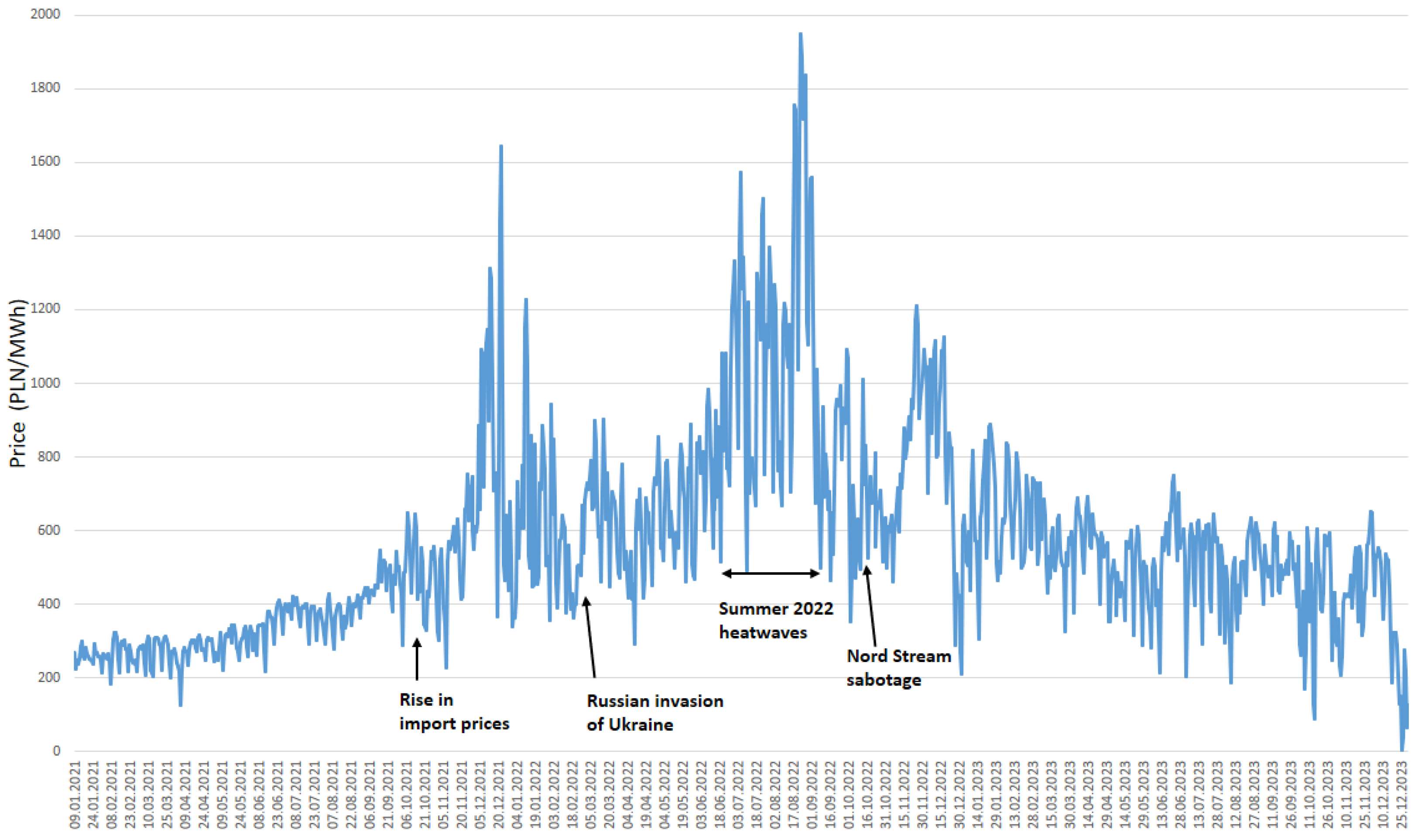
The last few years have shown directly how many factors influence energy prices and how unpredictable this market can be (Figure 2). The 3-year period chosen for the study (1 January 2021–31 December 2023) includes many phenomena of a random nature (black swans) like the conflict in Ukraine, diversions on the Nord Stream 1 and Nord Stream 2 pipelines, the embargo on coal imports from Russia, the introduction of the Fit for 55 rules in Europe, an intervention in imports of energy fuels, etc., which have a significant impact on energy prices (see also [58]).

Figure 2.
Average daily prices in the Polish electricity market January 2021–December 2023.
Even a preliminary analysis of the data indicated that all three types of anomalies described in the previous section were present during the study period, which has important implications for further research proceedings, including the choice of model quality metrics.
3.2. Error Metrics
Many absolute and relative measures are used to assess the quality of forecasts. Let be the actual value and be the forecast in period t, while n is the length of the time series. Among the classic evaluation measures there are [6,59,60,61,62]:
Mean Error (ME) as a bias measure:
Mean Square Error (MSE):
Root Mean Square Error (RMSE):
RMSE is sensitive to large differences between actual values and forecasts, which may be considered an advantage or a disadvantage. On the one hand, it is helpful in detecting significant but rare errors. But it may also be unstable when used as an optimization criterion. Therefore, it is often preferable to use the Mean Absolute Error (MAE):
which is resistant to rare large errors.
The above metrics are easy to interpret and useful in assessing the magnitude of errors. They may be supplemented by unit-less relative measures such as the Mean Absolute Percentage Error (MAPE) [63]:
The disadvantage of the measure is that for actual values, a equal or close to zero causes the MAPE value to increase to infinity. This problem may be bypassed in many ways. One of them is the use of the Symmetric Mean Absolute Percentage Error (sMAPE) [59,64,65]:
It is the average ratio of an absolute prediction error to the sum of the absolute values of the actual value and the forecast. This measure takes values in the range [0;2]. Unfortunately, this metric fails when prices and forecasts are close to zero.
Another relative measure that takes values in the interval [0; is the Mean Arc-tangent Absolute Percentage Error (MAAPE) [66]:
MAAPE is another modification of the MAPE measure. For small percentage deviations, the values of both measures are very similar, while for large deviations MAAPE tends toward π/2, while MAPE trends toward infinity. The interpretation of both measures is identical—the smaller the error, the better the forecast.
The division by zero is easier to avoid when the denominator depends on more data points and the measure is calculated from a longer period preceding the forecast, depending on the degree of data aggregation. It can be a week, a month, or a year. Here we can mention the normalized metrics of average forecast errors (NRMSE):
or NMAE (Mean Absolute Percentage Error) [59]:
The magnitude of individual errors proportionally affects the value of the NMAE. The measure is standardized by the average of the absolute values of electricity prices from the selected period of market operation, which practically excludes values close to or equal to zero.
Hyndman and Koehler [65] proposed to use the scaled errors for forecast accuracy, while in [6] authors recommended using the relative MAE (rMAE), which is calculated from an out-of-sample dataset:
where denotes a naïve forecast.
This measure assesses the predictive effectiveness of the model used as compared to the effectiveness of the naïve approach.
From a rich set of metrics of the accuracy of the model, the MAPE (Mean Percentage Error) metric [67] fits well into the characteristics of energy prices time series, i.e., the fact that energy prices vary in a wide range even during one day. However, some prices in the series were found to be very close to or equal to zero. For this reason, as a criterion for selecting and training the base model and assessing the quality of the results achieved, we finally decided to use the NMAE metric.
4. Preparation and the Conduct of the Experiment
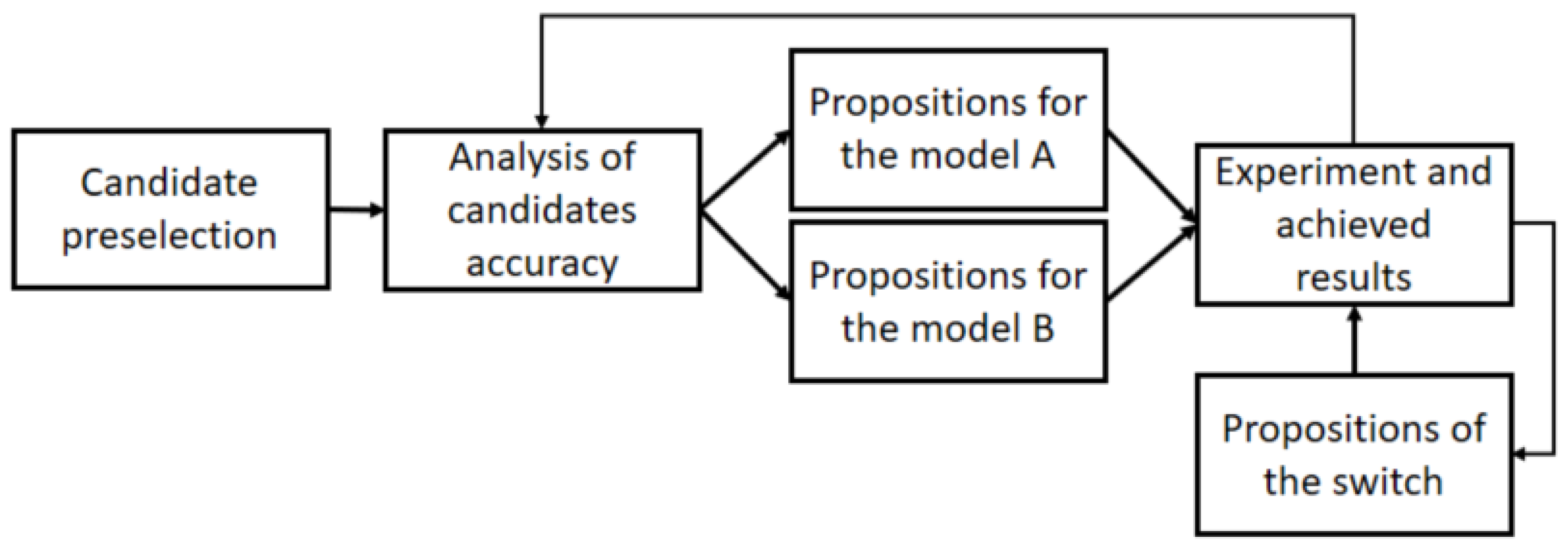
The entire flow of the research process is depicted in Figure 3.
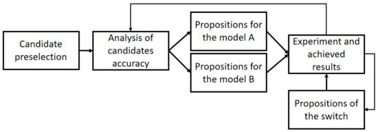
Figure 3.
Scheme of the research.
The first step of the procedure is the pre-selection of candidate methods, while he remaining steps are an iterative process of experimentally searching for the best models in both stable and anomalous periods and for a switch that controls the operation of the models. The following sections detail the implementation of the subsequent steps of the procedure.
The calculations were performed with Python scripts using the ML methods contained in the libraries scikit-learn and SciPy on a Dell Precision 5570 computer with a 12th Gen Intel(R) Core(TM) i7-12800H CPU and 32 GB RAM. R Studio was used for the statistical analysis of the results.
4.1. Candidate Pre-Selection
At the candidate pre-selection stage, based on a literature analysis, four ML methods were selected for further research: k-nearest neighbors (kNN), regression trees (RTs), random forests (RFs), and SVR.
According to the nonparametric kNN method, the forecast is formed as a smoothed value based on energy prices that correspond to k points in the space of explanatory variables which are in some sense the most similar to the point for which the forecast is made. The great advantage of this method is its simplicity of both calculation and interpretation. The disadvantage is the need to establish a fixed, time invariant number of neighbors. In addition, the smoothed value does not always reflect the actual relationship between the dependent variable and the independent variables. In forecasting electricity prices, kNN gives satisfactory results compared to other ML methods [68,69,70,71].
Nonparametric nonlinear regression trees exhibit advantages over classical prediction models like ARIMA because they do not require restrictions on error distributions, linearity, or variable types. The good quality of forecasts obtained via these methods contributes to their growing popularity [72,73]. The work [74] suggests that RTs perform better than classical models and no worse than methods based on neural networks. RT models are simple and explainable. They have few parameters as compared to classical models. In addition, they do not require as much historical information as models based on neural networks. This makes them more useful in dynamically changing market conditions. They have been successfully used to forecast prices and demand in the electricity market [62,75].
The problem of choosing the tree size is solved by introducing the concept of random forests (RFs), in which the final forecast is obtained by aggregating multiple individual forecasts calculated from various regression trees. The application of random forests improves the prediction accuracy as compared to single tree models [59,62,76,77,78]. In [23], it is demonstrated that RF-based forecasts are more accurate than those obtained using GBM (Gradient Boost Machines) or SVM/SVR (Support Vector Regression). Comparing the results of forecasting New York and Los Angeles gasoline daily spot prices based on the regression tree model, RF, and SVM, the authors of [79] obtained the lowest errors from the RF model.
Artificial neural networks have also demonstrated their usefulness in energy price prediction [16,80]. They enable an effective modeling of the complex relationships between input variables and energy prices, and they are able to account for non-stationarity, non-linearity, and fluctuations in the data. They have the ability to automatically extract features and learn from large amounts of data. However, there are also some limitations, such as the need for large amounts of training data, the complexity of the model, and the difficulty of explaining the results. Using ANNs was also considered as part of our research investigation, but was abandoned for two reasons:
- Outliers influence the quality of ANN performance [81] and most of authors recommend that they should be removed from the training data, which contradicts the aim of our study [82,83];
- Training ANNs requires a large amount of data, whereas anomalous values in the series under study are rare enough that there is not enough data to train the network.
In other words, ANNs are a good tool for building a general model, but not one whose purpose is precisely to account for outliers.
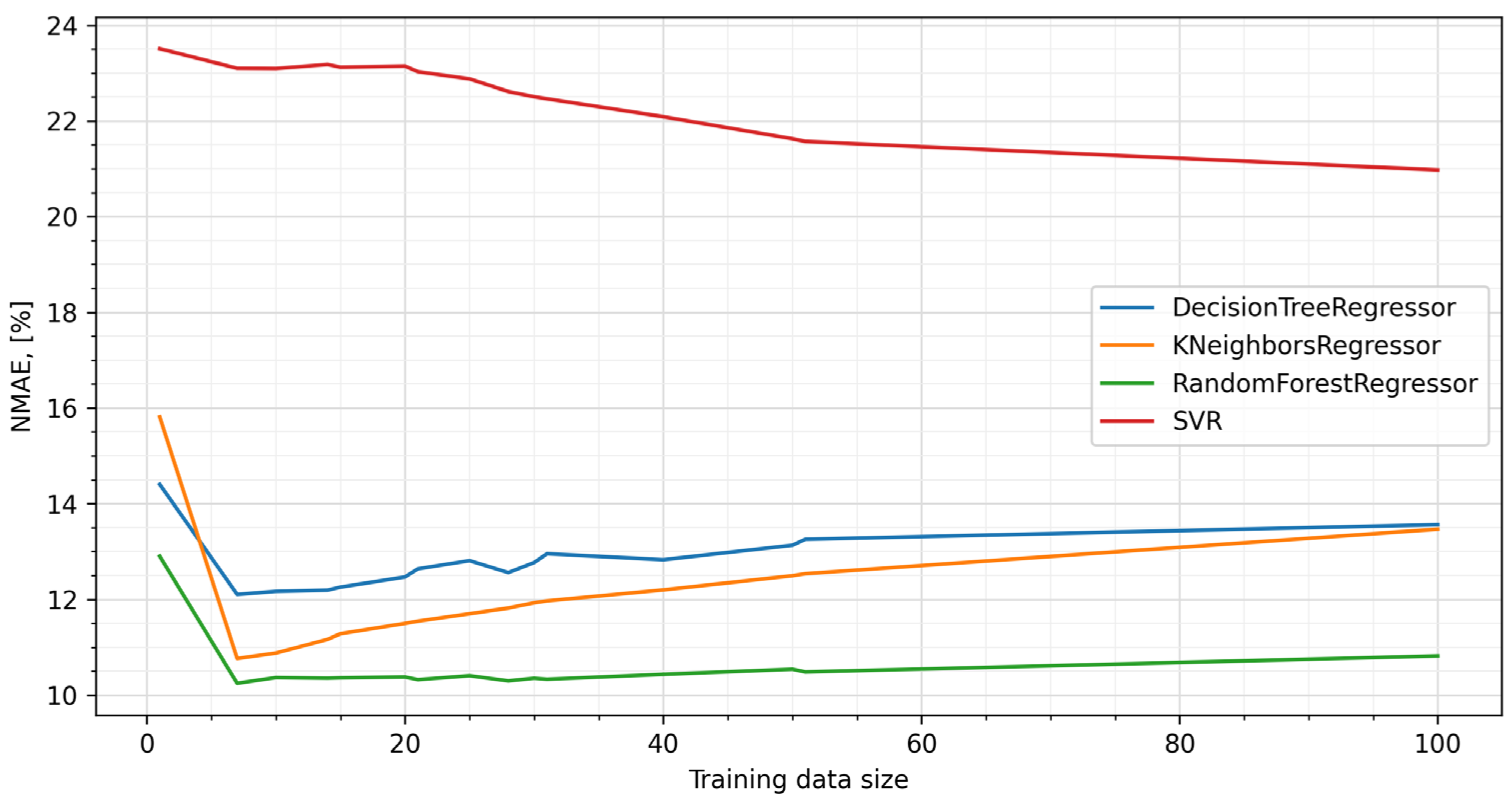
For each of the four methods described above, predictive models were built for a different number of days prior to prediction and the prediction errors rate NMAEs were calculated. The results of the comparison are shown in Figure 4.
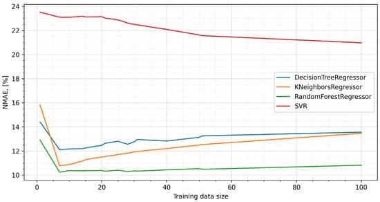
Figure 4.
Comparison of prediction errors (NMAE).
It is worth noting that, regardless of the length of the training data, the best results were obtained using RFs, and for three of the four methods the minimum prediction error occurred when the training set covered the period of eight days immediately preceding the day for which the prediction was made. Based on these results, random forests were used in the next steps of the experiment.
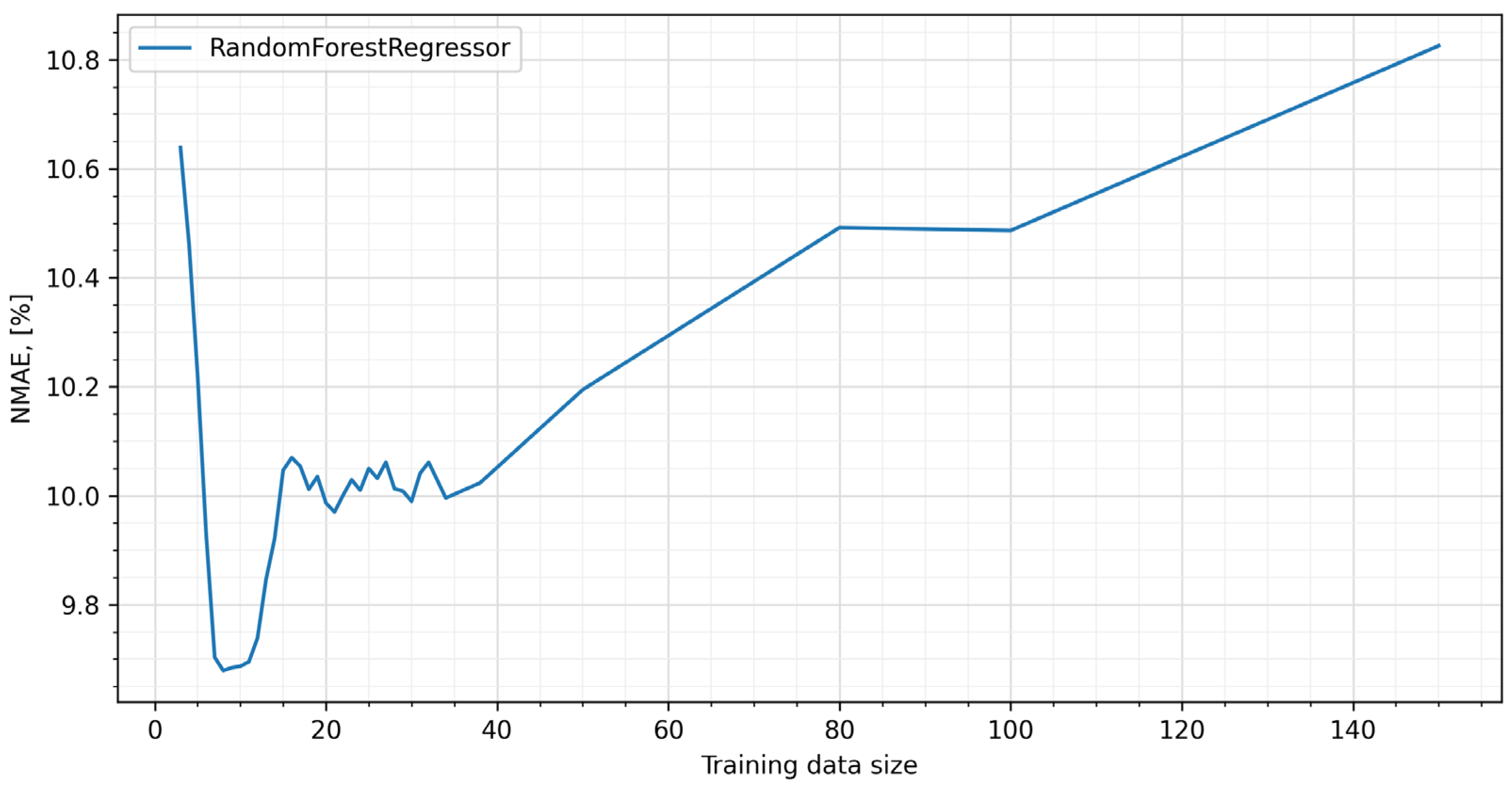
4.2. Random Forests Tuning
The next step of the procedure was to search for the parameters of the random forests that gave the best results. In the course of the study, it became apparent that the most significant influence on the quality of the prediction was the values occurring in the period immediately preceding the day for which the prediction was built (Figure 5).

Figure 5.
NMAE error for tuned RFs.
Both lengthening the learning set backward and learning based on other strategies, e.g., skip learning, caused the error to increase. These results confirm the observation that for a time series of prices, autocorrelation quickly disappears [9,74,84,85], which is due to seasonality and high market volatility. Thus, finally, the RF model with an 8-day period was adopted as the base model (model A in Figure 1).
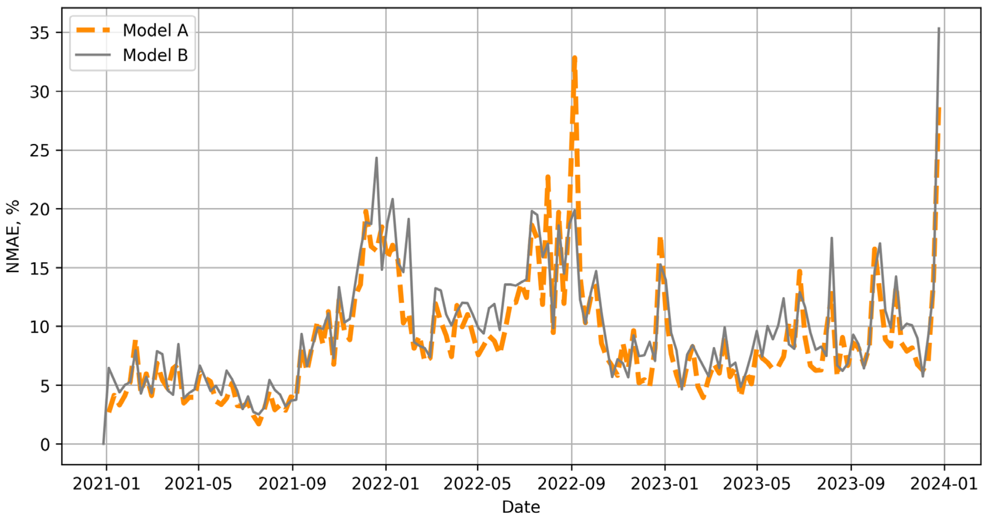
Searching for candidates for model B (a predictive model to be used during periods of anomaly) was based on a simple intuition that in a period of turbulence, past values play only a marginal role. In a subsequent series of experiments, it became apparent that an RF model trained on data from the three days preceding the prediction gave the best results in periods that were arbitrarily designated as anomalies (Figure 6).
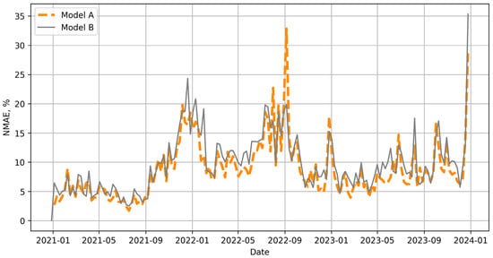
Figure 6.
Weekly NMAE error for 8 and 3-day RF models.
It can be seen that in some periods the 3-day model B produced significantly smaller errors than the 8-day model A, especially in the summer months of 2022. Thus, finally, for each successive hour of the following day, RFs were trained on the fly, based on data from the previous eight and three days.
4.3. Switch Design
The next step in the procedure shown in Figure 3 is to select and test different types of switches with different thresholds. The improvement in prediction quality depends on the indication of the correct switching time between models. A switch that is too sensitive will give false positive alarms and change the prediction to model B too often. A switch that is not sensitive enough will give mostly true-positive alarms but will miss some of the anomalies. It is a well-known problem of balance between recall and sensitivity in classification tasks. Three cases are therefore possible, the occurrence of which reduces the overall quality of the prediction:
- The switch will activate when there is no anomaly, and we will receive worse results from model B than if we used model A.
- The switch will not activate even though an anomaly has occurred, and we will receive worse results from model A than if we had used model B.
- The switch works correctly, but model B still gives worse results than A (there is no guarantee that when anomaly occurs model B will always give better results than A).
The switch should be tailored to the overall market situation. Since the concept of anomaly is relative [86] and depends on the circumstances, the design of the switch assumes, based on simple intuition, that it should switch calculations between models depending on the market situation, which can be assessed in different ways. Many approaches to setting the threshold are presented in the literature. Some authors set it up at a specified price level [87], fixed price change [88], or a fixed multiple of the standard deviation from the current prices [89]. Price spikes may be identified by various kinds of models [20].
Three types of switches were tested. The design of two was based directly on the definition of an anomaly given in Section 2.1. (The deviation—absolute or relative—of an observation is large enough that it is likely to be caused by the occurrence of a previously unaccounted-for factor). We assumed that if a certain fixed indicator is greater/less than a certain threshold, it is a signal of the occurrence of an anomaly. The first switch used the percentage change in the average daily price relative to the price a week earlier to avoid the influence of differences on individual days of the week (Equation (11)—denoted further as SMPP). The second one was based on the absolute change in the average daily price relative to the price a week earlier (Equation (12)—denoted further as SMP).
In the course of the experiments, it was observed that the prediction errors differed significantly for models A and B at certain times. This prompted us to test the less obvious idea of making the switch dependent on the quality of previous predictions. Therefore, the third switch operates according to Equation (13), (denoted further as SPC):
where
- t + 1—day of the prediction,
- P(t)—price on day t,
- —prediction of the 8-day model for the day t,
- —prediction of the 3-day model for the day t,
- T—a threshold of the switch.
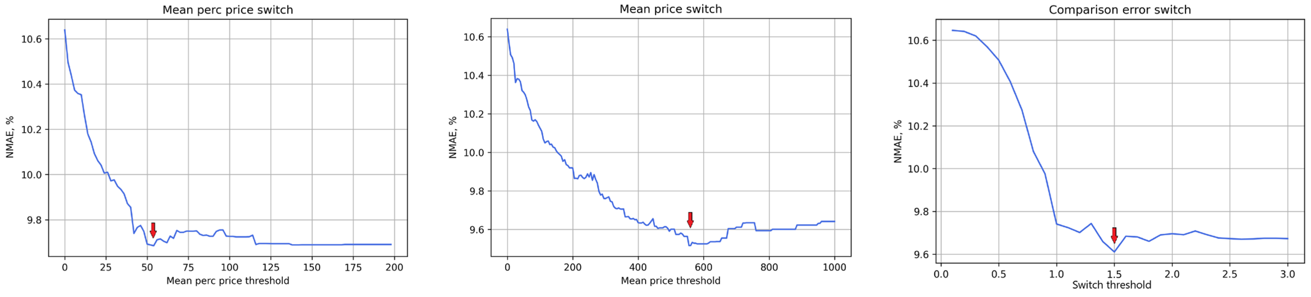
The threshold value for each switch can be interpreted as the sensitivity level of the switch. For each switch, the value that gives the best results in terms of achieving the smallest error for the hybrid model A + B (adaptive model) has been determined experimentally (marked by red arrows in Figure 7). For the individual switches, these are respectively TMPP = 54, TMP = 560, and TPC = 1.5, and these values have been used in all of the figures and calculations presented below.
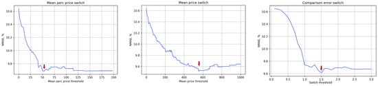
Figure 7.
Switch curves with marked values for minimal NMAE error for all data, from left to right: SMPP, SMP and SPC switches.
As can be seen, in every case the switch operates with a one-day delay. This delayed operation of the switches is due to the rules of the energy market itself, where contracts are closed the day before and no more transactions can be made during the settlement day. Thus, when closing contracts for the next day, we do not know the current prices (see also [6]).
5. Experiment Results
During the experiment, 8-day and 3-day random forests were taught for prediction of each hour of the following day. If the day was indicated by the switch as normal the forecast of the 8-day model was taken as the final one, if it was indicated as anomalous the 3-day model was taken. The forecast was calculated for each hour of the following day, both for models A and B separately and for the hybrid model A+B, with all three switches.
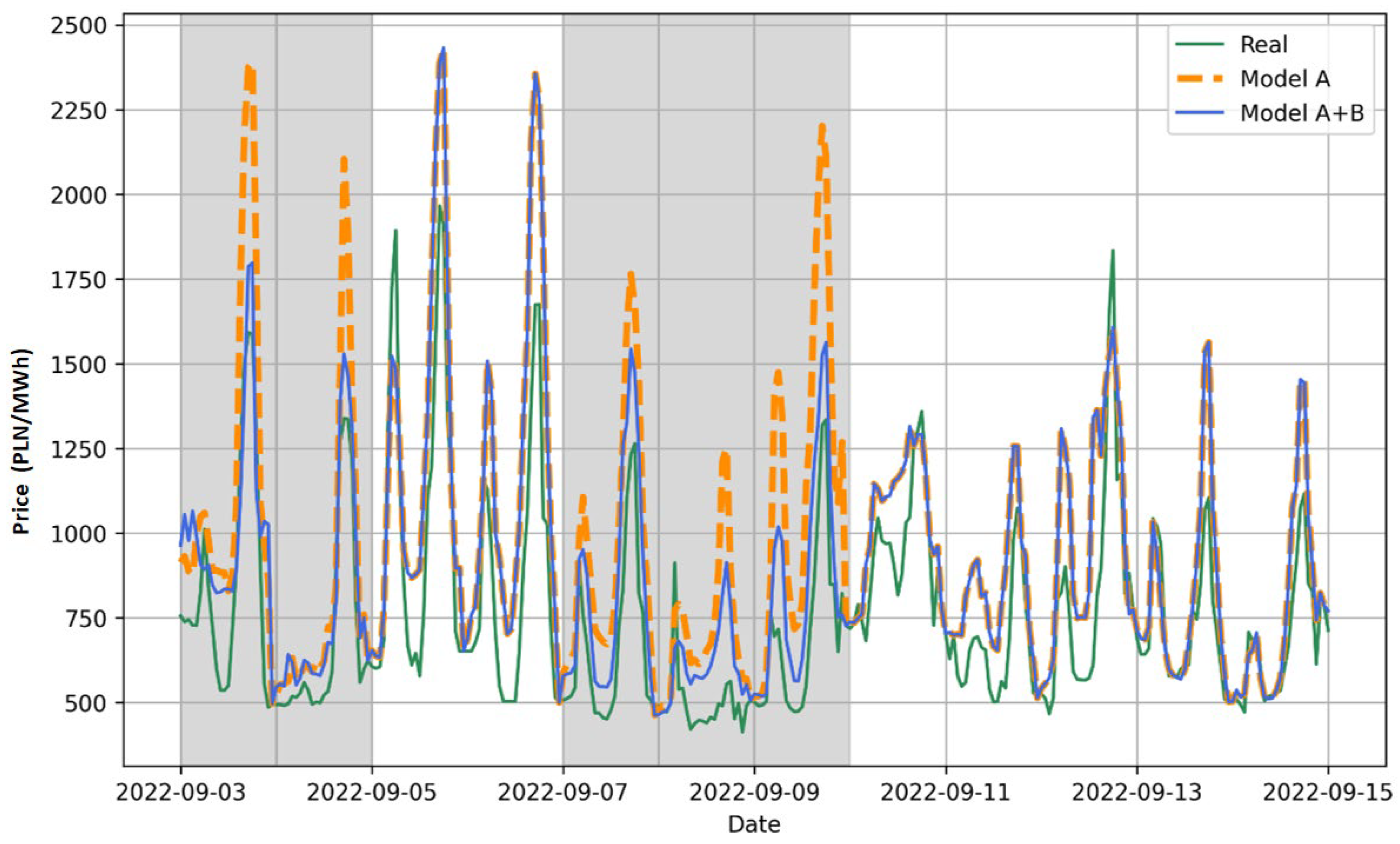
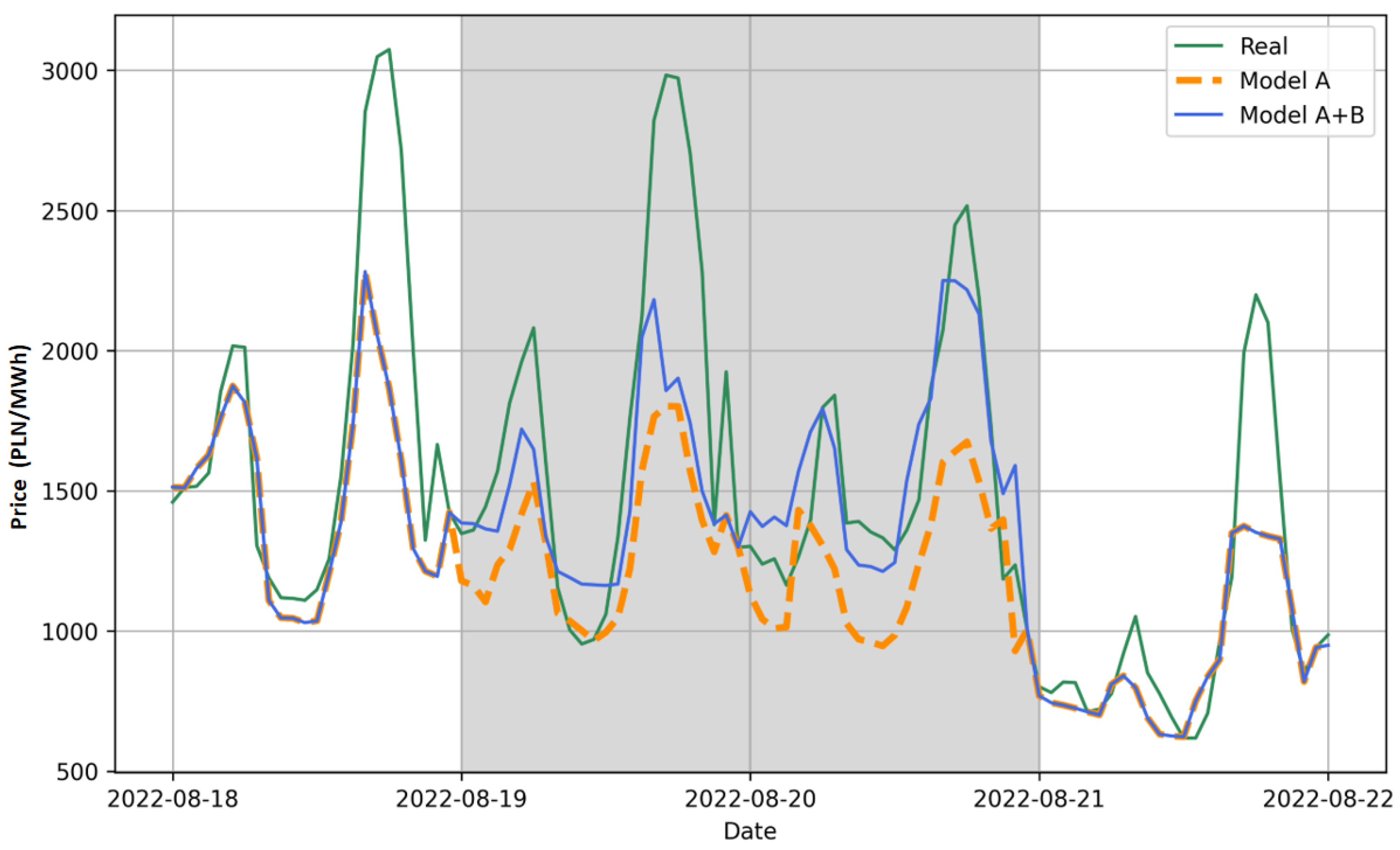
Sample visualizations of the correct operation of the model with the switches SMP and TMP = 560 for two periods (3–15 September 2022 and 18–22 September 2022) are shown in Figure 8 and Figure 9. Actual values are indicated by the green line, model A results by the orange line, and model B result by the blue line. Gray areas indicate periods classified as anomalies. Figure 8 shows the two anomaly periods 3–5 September and 7–10 September. During both anomalies, model B (3-day model) returned values smaller than model A (8-day model) and these were closer to the actual values. In turn, Figure 9 shows the anomaly period 19–21 September and during this anomaly, model B returned predicted values greater than model A, and these were also closer to the actual values.
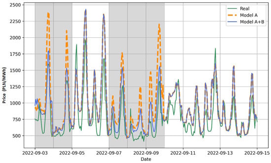
Figure 8.
An example of operation for model A and hybrid model (A+B) with switch SMP during the period of 3 September 2022–15 September 2022.
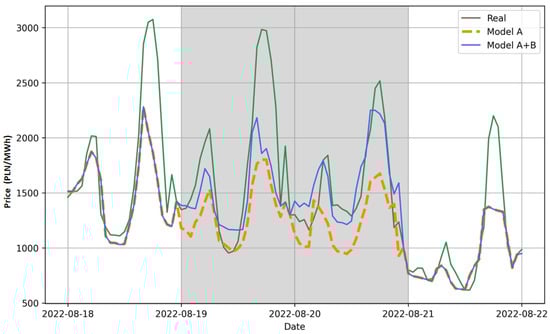
Figure 9.
An example of operation for model A and hybrid model (A+B) with switch SMP during the period of 18–22 September 2022.
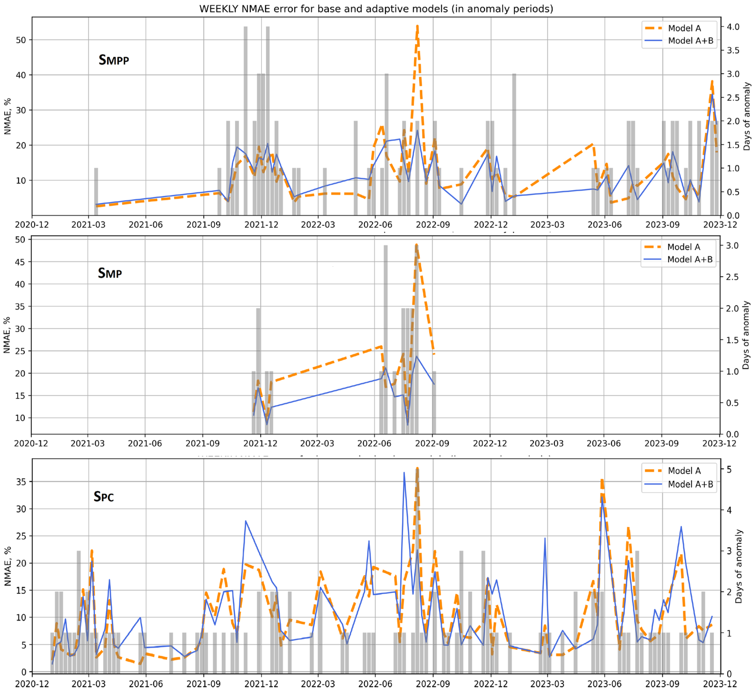
Figure 10 shows the weekly error values for models A and A + B (left scale) together with the anomaly periods (gray bars—right scale, indicates how many days per week were indicated as anomalies) for the three switches. It can be seen that regardless of the switch, anomalies were detected during December 2021 and the summer of 2022. It can also be seen that the switches operated with different sensitivities. The SPC switch indicated the highest number of anomalies (including in the calm 2021), but its false alarm errors were also the most frequent. Particularly for the March 2023 anomaly, model B gave significantly worse results than model A, indicating a failure of the SPC switch. At the same time, it is worth noting that the other two switches did not indicate anomalies at all during this period. The SMP switch was found to be the least sensitive, but in the periods of detected anomalies the A+B model was almost always better than model A. Note that the SMP switch indicated periods of anomalies only in 2022, while the other two indicated them even in 2021, which we considered generally calm, and in 2023. This means that the SMP and SPC switches work more flexibly and are correspondingly more sensitive during calmer periods and less sensitive during turbulences.
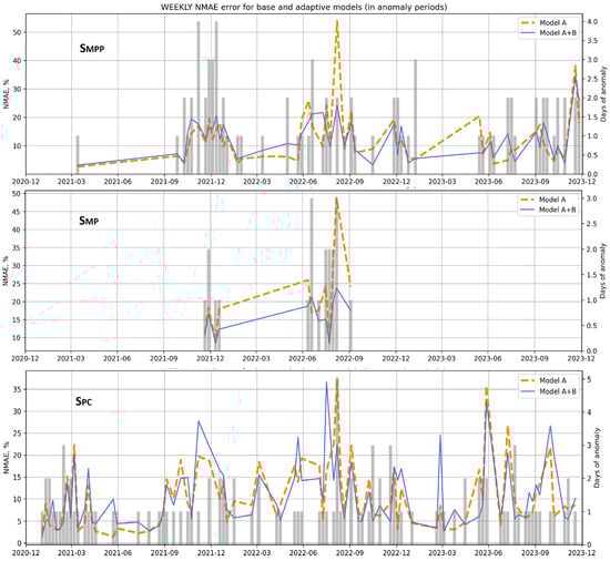
Figure 10.
Weekly comparison of NMAE errors of models during periods of anomalies for all three switches.
The results of the entire experiment are summarized in Table 2. The values shown in Table 2 are the daily averages of ex-post errors calculated, according to the rules of the day-ahead market, one day in advance, for the models considered. Although the measure of error used in experiment was the NMAE, Table 2 also includes values for the other measures of prediction quality described in Section 3.2. The last row of the table shows the number and percentage of days indicated as anomalous by each switch. The best values of error measures are marked in bold.
Table 2.
Models accuracy (test set).
It might be stated that for all the models, errors were not very high. However, regardless of the switch selected, the hybrid model offers lower errors than either the A or B models used independently. The 8-day model A exhibits a slightly higher bias than the model B, which means that its forecasts underestimate actual prices on the average. Meanwhile model B—despite having the lowest bias—has the remaining errors higher than model A and the adaptive model, for all the switches. This should not be seen as a surprise, because model B by its design minimizes the bias. Regardless of the chosen switch, the adaptive model efficiently reduces average errors.
Among the switches used, for nearly every error metric the lowest errors were obtained for the switch SPM. Predictions based on this model are characterized by the highest positive bias, which suggests an underestimation of predicted values. The remaining metrics also indicate that this approach is the most effective. By choosing this switch, we err by 54.05 PLN/MWH on average, which constitutes about 9.5% of the actual energy price, and the rMAE shows that models with this switch are more effective than the naïve seasonal prediction by 1 − 0.3636 = 63.64%. It is worth noting here that this switch indicated only 20 days (about 1.83% of the length of the entire period) as anomalies, and in all the periods indicated, model B was better than model A. This switch is therefore the least sensitive, but if it does indicate anomalies, it is not wrong, i.e., it switches to the model that gives the better forecast.
In the last three columns of the Table 2, the average prediction errors are separately shown for models A and B, covering only the periods that were identified as anomalous. For the switches SMP and SPC, all error metrics for model B were lower than for model A. In the anomalous periods identified by the least sensitive switch SMP, the prediction errors for model B were substantially lower than for model A. In general, high errors in this period result from atypical prices. This confirms the efficient identification of heightened volatility periods. On the other hand, low readings of rMAE confirm higher prediction efficiency for the adaptive model in the anomalous periods for both the A and B variants as compared to the naïve approach.
The preparation of a single forecast for the next day, i.e., the training of the 8-day model, the training of the 3-day model, and the selection of the model based on the switch value, is very fast. It is done in less than 1 s, which is absolutely sufficient for the decision-making process in the day-ahead market and allows the decision maker to simulate and consider various options.
6. Conclusions
Both specific and more general conclusions can be drawn from the implementation and results of the experiment. The specific conclusions concern the magnitude of the prediction errors of the time series under study for the entire period under study, as well as the anomaly periods. The use of the hybrid model has improved the overall quality of the energy price prediction, but this does not appear to be a main benefit. This is because the quality indicators of the total prediction have been improved to a relatively small extent, and this is due to the fact that the duration (number) of periods relative to the duration of the entire period under study is small (in the experiment carried out, depending on the switch used, it was between 1.83% and 9.95% of the total length of the series). The greater benefit of the proposed solution, which was confirmed by the experimental results, appears to be the correct (useful from the decision maker’s point of view) identification of anomalous periods and the achievement of a high degree of improvement during these periods.
Another conclusion to be drawn from the experiment results concerns the switch design. As can be seen, different results were obtained for each of the switches used (different number of anomaly period indications and different switch efficiency). This shows that the choice of switch, in addition to the choice of the models themselves, has a decisive impact on the performance of the proposed hybrid solution. Depending on the design and parameters of the switch, the whole model may be more or less sensitive to deviations of the forecast value. On the one hand, this makes it necessary to test different types of switches and, on the other hand, offers the possibility to better adapt the model’s performance to the user’s preferences. Depending on these, its performance may be more or less sensitive depending on the set level of volatility of the predicted value.
A more general conclusion is that a model that performs well most of the time gives poorer results in periods that do not fit its characteristics, and it can and should be replaced by another model specifically designed for such cases. In the case of non-hybrid (homogeneous) forecasting models, improving forecasting during periods of anomalies can lead to poorer forecast quality in periods outside of them. With the proposed approach, improving the quality of forecasting in anomalous periods can be done independently of forecasting in stable periods.
A limitation of the proposed hybrid model is the larger number of parameters compared to other proposed hybrid models. In addition to the parameters related to the individual models, there are additional ones related to the functioning of the switch. This increases the number of possible combinations (model A, model B, switch) and thus increases the time-consumption and cost of building the entire model. Another limitation of the model presented is its inability to respond to very short-lived anomalies (lasting hours) due to the switch design, which is based on daily averages. This will also be the subject of further work.
The positive results of the experiment also indicate further lines of work. These will aim to test the usefulness of the proposed approach for other time series that contain periods defined as anomalous. If positive results are obtained, the next research step will be to try to generalize the approach and propose a general framework for building hybrid ML models based on the principle of dividing the series into sub-periods with different characteristics that can be automatically identified. The results of the experiment also showed that the use of different switches is particularly important to improve the quality of the forecast in periods identified as anomalies, which may be more relevant from the decision maker’s point of view than general accuracy. This extends the model to include subjective factors such as the preferences of the decision maker. Therefore, we also plan to investigate the relationship between the proposed hybrid model design and the level of risk propensity/aversion indicated by the decision maker.
It is worth noting that the procedure in Figure 3 does not have a STOP. This is because we do not know whether there is another combination of models and switch that will produce even better prediction results, unless we reach the level of an ideal prediction. This is due to the possibility of using different ML models for different types of sub-periods and the possibility of different switch designs, including those that are based on more complex relationships than those used in the experiment. Therefore, the space of possible solutions that needs to be explored is very large.
Author Contributions
Conceptualization, K.P., A.G.-G. and K.K.; methodology, K.P., A.G.-G. and K.K.; software, K.P. and A.G.-G.; formal analysis, K.P., A.G.-G. and K.K.; investigation, K.P., A.G.-G. and K.K.; resources, K.P.; data curation, K.P.; writing—original draft preparation, K.P., A.G.-G. and K.K.; writing—review and editing, K.P., A.G.-G. and K.K.; visualization, K.P. All authors have read and agreed to the published version of the manuscript.
Funding
This research received no external funding.
Data Availability Statement
All data used in the study are publicly available.
Conflicts of Interest
The authors declare no conflicts of interest.
References
- Beltrán, S.; Castro, A.; Irizar, I.; Naveran, G.; Yeregui, I. Framework for collaborative intelligence in forecasting day-ahead electricity price. Appl. Energy 2022, 306, 118049. [Google Scholar] [CrossRef]
- Dudek, G.; Piotrowski, P.; Baczyński, D. Intelligent Forecasting and Optimization in Electrical Power Systems: Advances in Models and Applications. Energies 2023, 16, 3024. [Google Scholar] [CrossRef]
- Ganczarek-Gamrot, A.; Krężołek, D.; Trzpiot, G. Using EVT to Assess Risk on Energy Market; Springer: Berlin/Heidelberg, Germany, 2021; pp. 57–64. [Google Scholar]
- Weron, R. Modeling and Forecasting Electricity Loads and Prices; John Wiley & Sons, Inc.: West Sussex, UK, 2006; ISBN 9780470057537. [Google Scholar]
- Kostrzewski, M.; Kostrzewska, J. Probabilistic electricity price forecasting with Bayesian stochastic volatility models. Energy Econ. 2019, 80, 610–620. [Google Scholar] [CrossRef]
- Lago, J.; Marcjasz, G.; De Schutter, B.; Weron, R. Forecasting day-ahead electricity prices: A review of state-of-the-art algorithms, best practices and an open-access benchmark. Appl. Energy 2021, 293, 116983. [Google Scholar] [CrossRef]
- Wang, Z.; Wang, Y.; Zeng, R.; Srinivasan, R.S.; Ahrentzen, S. Random Forest based hourly building energy prediction. Energy Build. 2018, 171, 11–25. [Google Scholar] [CrossRef]
- Uniejewski, B.; Maciejowska, K. LASSO principal component averaging: A fully automated approach for point forecast pooling. Int. J. Forecast. 2023, 39, 1839–1852. [Google Scholar] [CrossRef]
- Chodakowska, E.; Nazarko, J.; Nazarko, Ł. ARIMA Models in Electrical Load Forecasting and Their Robustness to Noise. Energies 2021, 14, 7952. [Google Scholar] [CrossRef]
- Koopman, S.J.; Ooms, M.; Carnero, M.A. Periodic Seasonal Reg-ARFIMA–GARCH Models for Daily Electricity Spot Prices. J. Am. Stat. Assoc. 2007, 102, 16–27. [Google Scholar] [CrossRef]
- Ganczarek-Gamrot, A. Forecast of prices and volatility on the Day Ahead Market. Econometrics 2013, 1, 111–120. [Google Scholar]
- Kostrzewski, M.; Kostrzewska, J. The Impact of Forecasting Jumps on Forecasting Electricity Prices. Energies 2021, 14, 336. [Google Scholar] [CrossRef]
- Gianfreda, A.; Ravazzolo, F.; Rossini, L. Comparing the forecasting performances of linear models for electricity prices with high RES penetration. Int. J. Forecast. 2020, 36, 974–986. [Google Scholar] [CrossRef]
- Ziel, F.; Weron, R. Day-ahead electricity price forecasting with high-dimensional structures: Univariate vs. multivariate modeling frameworks. Energy Econ. 2018, 70, 396–420. [Google Scholar] [CrossRef]
- Lago, J.; De Ridder, F.; De Schutter, B. Forecasting spot electricity prices: Deep learning approaches and empirical comparison of traditional algorithms. Appl. Energy 2018, 221, 386–405. [Google Scholar] [CrossRef]
- Olivares, K.G.; Challu, C.; Marcjasz, G.; Weron, R.; Dubrawski, A. Neural basis expansion analysis with exogenous variables: Forecasting electricity prices with NBEATSx. Int. J. Forecast. 2023, 39, 884–900. [Google Scholar] [CrossRef]
- Wang, D.; Gryshova, I.; Kyzym, M.; Salashenko, T.; Khaustova, V.; Shcherbata, M. Electricity Price Instability over Time: Time Series Analysis and Forecasting. Sustainability 2022, 14, 9081. [Google Scholar] [CrossRef]
- Chai, S.; Li, Q.; Abedin, M.Z.; Lucey, B.M. Forecasting electricity prices from the state-of-the-art modeling technology and the price determinant perspectives. Res. Int. Bus. Financ. 2024, 67, 102132. [Google Scholar] [CrossRef]
- El-Azab, H.-A.I.; Swief, R.A.; El-Amary, N.H.; Temraz, H.K. Machine and deep learning approaches for forecasting electricity price and energy load assessment on real datasets. Ain Shams Eng. J. 2024, 15, 102613. [Google Scholar] [CrossRef]
- Chen, C.; Liu, L.-M. Joint Estimation of Model Parameters and Outlier Effects in Time Series. J. Am. Stat. Assoc. 1993, 88, 284. [Google Scholar] [CrossRef]
- Meyer-Brandis, T.; Tankov, P. Multi-factor jump-diffusion models of electricity prices. Int. J. Theor. Appl. Financ. 2008, 11, 503–528. [Google Scholar] [CrossRef]
- Tsay, R.S. Testing and Modeling Threshold Autoregressive Processes. J. Am. Stat. Assoc. 1989, 84, 231–240. [Google Scholar] [CrossRef]
- Hamilton, J.D. Analysis of time series subject to changes in regime. J. Econom. 1990, 45, 39–70. [Google Scholar] [CrossRef]
- Janczura, J.; Weron, R. An empirical comparison of alternate regime-switching models for electricity spot prices. Energy Econ. 2010, 32, 1059–1073. [Google Scholar] [CrossRef]
- Misiorek, A.; Trueck, S.; Weron, R. Point and Interval Forecasting of Spot Electricity Prices: Linear vs. Non-Linear Time Series Models. Stud. Nonlinear Dyn. Econom. 2006, 10, 1362. [Google Scholar] [CrossRef]
- Fan, S.; Chen, L.; Lee, W.J. Machine learning based switching model for electricity load forecasting. Energy Convers. Manag. 2008, 49, 1331–1344. [Google Scholar] [CrossRef]
- Hawkins, D.M. Identification of Outliers; Chapman & Hall: London, UK, 1980. [Google Scholar]
- Kanamura, T.; Ōhashi, K. A structural model for electricity prices with spikes: Measurement of spike risk and optimal policies for hydropower plant operation. Energy Econ. 2007, 29, 1010–1032. [Google Scholar] [CrossRef]
- Aguinis, H.; Gottfredson, R.K.; Joo, H. Best-Practice Recommendations for Defining, Identifying, and Handling Outliers. Organ. Res. Methods 2013, 16, 270–301. [Google Scholar] [CrossRef]
- Ranga Suri, N.N.R.; Murty, M.N.; Athithan, G. Outlier Detection: Techniques and Applications; Intelligent Systems Reference Library; Springer International Publishing: Cham, Switzerland, 2019; Volume 155, ISBN 978-3-030-05125-9. [Google Scholar]
- Lee, J.; Cho, Y. National-scale electricity peak load forecasting: Traditional, machine learning, or hybrid model? Energy 2022, 239, 122366. [Google Scholar] [CrossRef]
- Amjady, N. Short-Term Electricity Price Forecasting. In Electric Power Systems: Advanced Forecasting Techniques and Optimal Generation Scheduling; Zhao, Y., Xu, J., Wu, J., Eds.; CRC Press: Boca Raton, FL, USA, 2017. [Google Scholar]
- Sun, L.; Zhou, K.; Zhang, X.; Yang, S. Outlier Data Treatment Methods Toward Smart Grid Applications. IEEE Access 2018, 6, 39849–39859. [Google Scholar] [CrossRef]
- Agnello, L.; Castro, V.; Hammoudeh, S.; Sousa, R.M. Global factors, uncertainty, weather conditions and energy prices: On the drivers of the duration of commodity price cycle phases. Energy Econ. 2020, 90, 104862. [Google Scholar] [CrossRef]
- Maciejowska, K.; Nitka, W.; Weron, T. Enhancing load, wind and solar generation for day-ahead forecasting of electricity prices. Energy Econ. 2021, 99, 105273. [Google Scholar] [CrossRef]
- Janczura, J.; Trück, S.; Weron, R.; Wolff, R.C. Identifying spikes and seasonal components in electricity spot price data: A guide to robust modeling. Energy Econ. 2013, 38, 96–110. [Google Scholar] [CrossRef]
- Nowotarski, J.; Weron, R. Recent advances in electricity price forecasting: A review of probabilistic forecasting. Renew. Sustain. Energy Rev. 2018, 81, 1548–1568. [Google Scholar] [CrossRef]
- Lu, X.; Dong, Z.Y.; Li, X. Electricity market price spike forecast with data mining techniques. Electr. Power Syst. Res. 2005, 73, 19–29. [Google Scholar] [CrossRef]
- Christensen, T.M.; Hurn, A.S.; Lindsay, K.A. Forecasting spikes in electricity prices. Int. J. Forecast. 2012, 28, 400–411. [Google Scholar] [CrossRef]
- Zhang, R.; Li, G.; Ma, Z. A Deep Learning Based Hybrid Framework for Day-Ahead Electricity Price Forecasting. IEEE Access 2020, 8, 143423–143436. [Google Scholar] [CrossRef]
- Zhao, Y.; Xu, J.; Wu, J. A New Method for Bad Data Identification of Oilfield System Based on Enhanced Gravitational Search-Fuzzy C-Means Algorithm. IEEE Trans. Ind. Inform. 2019, 15, 5963–5970. [Google Scholar] [CrossRef]
- Bibi, N.; Shah, I.; Alsubie, A.; Ali, S.; Lone, S.A. Electricity Spot Prices Forecasting Based on Ensemble Learning. IEEE Access 2021, 9, 150984–150992. [Google Scholar] [CrossRef]
- Ahmad, T.; Chen, H. Nonlinear autoregressive and random forest approaches to forecasting electricity load for utility energy management systems. Sustain. Cities Soc. 2019, 45, 460–473. [Google Scholar] [CrossRef]
- Angamuthu Chinnathambi, R.; Mukherjee, A.; Campion, M.; Salehfar, H.; Hansen, T.; Lin, J.; Ranganathan, P. A Multi-Stage Price Forecasting Model for Day-Ahead Electricity Markets. Forecasting 2018, 1, 26–46. [Google Scholar] [CrossRef]
- Filho, J.C.R.; de, M. Affonso, C.; de Oliveira, R.C.L. Energy price prediction multi-step ahead using hybrid model in the Brazilian market. Electr. Power Syst. Res. 2014, 117, 115–122. [Google Scholar] [CrossRef]
- Gulay, E.; Duru, O. Hybrid modeling in the predictive analytics of energy systems and prices. Appl. Energy 2020, 268, 114985. [Google Scholar] [CrossRef]
- Amjady, N.; Keynia, F. Day ahead price forecasting of electricity markets by a mixed data model and hybrid forecast method. Int. J. Electr. Power Energy Syst. 2008, 30, 533–546. [Google Scholar] [CrossRef]
- Zhang, J.; Tan, Z.; Wei, Y. An adaptive hybrid model for short term electricity price forecasting. Appl. Energy 2020, 258, 114087. [Google Scholar] [CrossRef]
- Wan, C.; Xu, Z.; Wang, Y.; Dong, Z.Y.; Wong, K.P. A Hybrid Approach for Probabilistic Forecasting of Electricity Price. IEEE Trans. Smart Grid 2014, 5, 463–470. [Google Scholar] [CrossRef]
- Gomez, W.; Wang, F.-K.; Lo, S.-C. A hybrid approach based machine learning models in electricity markets. Energy 2024, 289, 129988. [Google Scholar] [CrossRef]
- Krishna, G.J.; Ravi, V. Evolutionary computing applied to customer relationship management: A survey. Eng. Appl. Artif. Intell. 2016, 56, 30–59. [Google Scholar] [CrossRef]
- Bates, J.M.; Granger, C.W.J. The Combination of Forecasts. J. Oper. Res. Soc. 1969, 20, 451–468. [Google Scholar] [CrossRef]
- Xiao, Y.; Xiao, J.; Wang, S. A hybrid model for time series forecasting. Hum. Syst. Manag. 2012, 31, 133–143. [Google Scholar] [CrossRef]
- Abbasimehr, H.; Behboodi, A.; Bahrini, A. A novel hybrid model to forecast seasonal and chaotic time series. Expert Syst. Appl. 2024, 239, 122461. [Google Scholar] [CrossRef]
- Luo, Z.; Guo, W.; Liu, Q.; Zhang, Z. A hybrid model for financial time-series forecasting based on mixed methodologies. Expert Syst. 2021, 38, e12633. [Google Scholar] [CrossRef]
- Yang, Y.; Fan, C.; Xiong, H. A novel general-purpose hybrid model for time series forecasting. Appl. Intell. 2022, 52, 2212–2223. [Google Scholar] [CrossRef] [PubMed]
- Khashei, M.; Bijari, M. An artificial neural network (p, d, q) model for timeseries forecasting. Expert Syst. Appl. 2010, 37, 479–489. [Google Scholar] [CrossRef]
- Energy Price Rise Since 2021. Available online: https://www.consilium.europa.eu/en/infographics/energy-prices-2021/ (accessed on 5 May 2024).
- Pórtoles, J.; González, C.; Moguerza, J. Electricity Price Forecasting with Dynamic Trees: A Benchmark Against the Random Forest Approach. Energies 2018, 11, 1588. [Google Scholar] [CrossRef]
- vom Scheidt, F.; Medinová, H.; Ludwig, N.; Richter, B.; Staudt, P.; Weinhardt, C. Data analytics in the electricity sector—A quantitative and qualitative literature review. Energy AI 2020, 1, 100009. [Google Scholar] [CrossRef]
- Tschora, L.; Pierre, E.; Plantevit, M.; Robardet, C. Electricity price forecasting on the day-ahead market using machine learning. Appl. Energy 2022, 313, 118752. [Google Scholar] [CrossRef]
- González, C.; Mira-McWilliams, J.; Juárez, I. Important variable assessment and electricity price forecasting based on regression tree models: Classification and regression trees, Bagging and Random Forests. IET Gener. Transm. Distrib. 2015, 9, 1120–1128. [Google Scholar] [CrossRef]
- Vivas, E.; Allende-Cid, H.; Salas, R. A systematic review of statistical and machine learning methods for electrical power forecasting with reported mape score. Entropy 2020, 22, 1412. [Google Scholar] [CrossRef]
- Chen, Z.; Yang, Y. Assessing forecast accuracy measures. Prepr. Ser. 2004, 1–26. [Google Scholar]
- Hyndman, R.J.; Koehler, A.B. Another look at measures of forecast accuracy. Int. J. Forecast. 2006, 22, 679–688. [Google Scholar] [CrossRef]
- Kim, S.; Kim, H. A new metric of absolute percentage error for intermittent demand forecasts. Int. J. Forecast. 2016, 32, 669–679. [Google Scholar] [CrossRef]
- St-Aubin, P.; Agard, B. Precision and Reliability of Forecasts Performance Metrics. Forecasting 2022, 4, 882–903. [Google Scholar] [CrossRef]
- Ashfaq, T.; Javaid, N. Short-Term Electricity Load and Price Forecasting using Enhanced KNN. In Proceedings of the 2019 International Conference on Frontiers of Information Technology (FIT), Islamabad, Pakistan, 16–18 December 2019; pp. 266–2665. [Google Scholar]
- Ali, M.; Khan, Z.A.; Mujeeb, S.; Abbas, S.; Javaid, N. Short-Term Electricity Price and Load Forecasting using Enhanced Support Vector Machine and K-Nearest Neighbor. In Proceedings of the 2019 Sixth HCT Information Technology Trends (ITT), Ras Al Khaimah, United Arab Emirates, 20–21 November 2019; pp. 79–83. [Google Scholar] [CrossRef]
- Yang, C.C.; Soh, C.S.; Yap, V.V. A systematic approach in appliance disaggregation using k-nearest neighbours and naive Bayes classifiers for energy efficiency. Energy Effic. 2018, 11, 239–259. [Google Scholar] [CrossRef]
- Aimal, S.; Javaid, N.; Islam, T.; Khan, W.Z.; Aalsalem, M.Y.; Sajjad, H. An Efficient CNN and KNN Data Analytics for Electricity Load Forecasting in the Smart Grid; Springer: Cham, Switzerland, 2019; pp. 592–603. [Google Scholar]
- Fata, E.; Kadota, I.; Schneider, I. Comparison of Classical and Nonlinear Models for Short-Term Electricity Price Prediction. arXiv 2018, arXiv:1805.05431. [Google Scholar]
- Time Series Forecasting Using Tree Based Methods. J. Stat. Appl. Probab. 2021, 10, 229–244. [CrossRef]
- Dudek, G. Short-Term Load Forecasting Using Random Forests; Springer: Berlin/Heidelberg, Germany, 2015; pp. 821–828. [Google Scholar]
- Dudek, G. A Comprehensive Study of Random Forest for Short-Term Load Forecasting. Energies 2022, 15, 7547. [Google Scholar] [CrossRef]
- Lahouar, A.; Ben Hadj Slama, J. Day-ahead load forecast using random forest and expert input selection. Energy Convers. Manag. 2015, 103, 1040–1051. [Google Scholar] [CrossRef]
- Mei, J.; He, D.; Harley, R.; Habetler, T.; Qu, G. A random forest method for real-time price forecasting in New York electricity market. In Proceedings of the 2014 IEEE PES General Meeting|Conference & Exposition, National Harbor, MD, USA, 27–31 July 2014; pp. 1–5. [Google Scholar]
- Romero, Á.; Dorronsoro, J.R.; Díaz, J. Day-Ahead Price Forecasting for the Spanish Electricity Market. Int. J. Interact. Multimed. Artif. Intell. 2019, 5, 42. [Google Scholar] [CrossRef]
- Sofianos, E.; Zaganidis, E.; Papadimitriou, T.; Gogas, P. Forecasting East and West Coast Gasoline Prices with Tree-Based Machine Learning Algorithms. Energies 2024, 17, 1296. [Google Scholar] [CrossRef]
- Catalão, J.P.S.; Mariano, S.J.P.S.; Mendes, V.M.F.; Ferreira, L.A.F.M. Short-term electricity prices forecasting in a competitive market: A neural network approach. Electr. Power Syst. Res. 2007, 77, 1297–1304. [Google Scholar] [CrossRef]
- Khamis, A.; Ismail, Z.; Haron, K.; Mohamm, A.T. The Effects of Outliers Data on Neural Network Performance. J. Appl. Sci. 2005, 5, 1394–1398. [Google Scholar] [CrossRef]
- Liano, K. Robust error measure for supervised neural network learning with outliers. IEEE Trans. Neural Netw. 1996, 7, 246–250. [Google Scholar] [CrossRef] [PubMed]
- Sandbhor, S.; Chaphalkar, N.B. Impact of Outlier Detection on Neural Networks Based Property Value Prediction; Springer: Singapore, 2019; pp. 481–495. [Google Scholar]
- Mestre, G.; Portela, J.; Muñoz San Roque, A.; Alonso, E. Forecasting hourly supply curves in the Italian Day-Ahead electricity market with a double-seasonal SARMAHX model. Int. J. Electr. Power Energy Syst. 2020, 121, 106083. [Google Scholar] [CrossRef]
- Borovkova, S.; Schmeck, M.D. Electricity price modeling with stochastic time change. Energy Econ. 2017, 63, 51–65. [Google Scholar] [CrossRef]
- Foorthuis, R. On the nature and types of anomalies: A review of deviations in data. Int. J. Data Sci. Anal. 2021, 12, 297–331. [Google Scholar] [CrossRef]
- Lapuerta, C.; Harris, D. Recomendations for the Dutch Electricity Market; The Brattle Group, Ltd.: London, UK, 2001. [Google Scholar]
- Bierbrauer, M.; Truck, S.; Weron, R. Modeling Electricity Prices with Regime Switching Models Electricity Spot Prices: Markets and Models; Lecture Notes in Computer Science; Springer: Berlin/Heidelberg, Germany, 2004; Volume 3039, pp. 859–867. [Google Scholar]
- Weron, R.; Bierbrauer, M.; Trück, S. Modeling electricity prices: Jump diffusion and regime switching. Phys. A Stat. Mech. Its Appl. 2004, 336, 39–48. [Google Scholar] [CrossRef]
Disclaimer/Publisher’s Note: The statements, opinions, and data contained in all publications are solely those of the individual author(s) and contributor(s) and not of MDPI and/or the editor(s). MDPI and/or the editor(s) disclaim responsibility for any injury to people or property resulting from any ideas, methods, instructions, or products referred to in the content. |
Disclaimer/Publisher’s Note: The statements, opinions and data contained in all publications are solely those of the individual author(s) and contributor(s) and not of MDPI and/or the editor(s). MDPI and/or the editor(s) disclaim responsibility for any injury to people or property resulting from any ideas, methods, instructions or products referred to in the content. |
© 2024 by the authors. Licensee MDPI, Basel, Switzerland. This article is an open access article distributed under the terms and conditions of the Creative Commons Attribution (CC BY) license (https://creativecommons.org/licenses/by/4.0/).