Article

Do Structural Transformations in the Energy Sector Help to Achieve Decarbonization? Evidence from the World’s Top Five Green Leaders

1
Department of Economics, Lahore College for Women University, Lahore 23570, Pakistan
2
Department of Economics, Division of Management and Administrative Science, University of Education, Lahore 54770, Pakistan
3
Department of Economics and Management Sciences, NED University of Engineering and Technology, Karachi 75270, Pakistan
4
UNEC Research Center for Monetary and Financial Technologies, Azerbaijan State University of Economics, Baku AZ 1001, Azerbaijan
5
School of Economics and Business, Western Caspian University, Baku AZ 1033, Azerbaijan
*
Author to whom correspondence should be addressed.
Energies 2024, 17(18), 4600; https://doi.org/10.3390/en17184600
Submission received: 29 July 2024 / Revised: 19 August 2024 / Accepted: 9 September 2024 / Published: 13 September 2024
(This article belongs to the Special Issue Energy Economics, Finance and Policy towards Sustainable Energy)

Abstract

:
The purpose of this study is to examine the role of structural transformation in the energy sector to accelerate the decarbonization process in the world’s top five green leaders, Germany, Canada, Sweden, Denmark, and Poland. To test this empirically, we collected annual data from a panel of the top five green leaders from 2000–2023. A key contribution of our study lies in assessing multiple critical metrics, including CO2 emissions, carbon intensity, carbon intensity of electricity, production-based carbon emissions, and consumption-based carbon emissions, to capture holistic progress towards carbon neutrality. We applied the augmented mean group (AMG) model to estimate the long-term results. The Dumitrescu–Hurlin test is used to test the causal relationship among the modeled variables. The findings of the AMG model reveal that renewable energy production and consumption significantly reduce CO2 emissions, production-based CO2 emissions, consumption-based CO2 emissions, carbon intensity, and the carbon intensity of electricity. Conversely, fossil-fuel-derived energy exacerbates these metrics. However, the impact of these energy sources varies by country in terms of their magnitude. The outcomes of the Dumitrescu–Hurlin test indicate that a bidirectional causality exists between renewable energy production and CO2 emissions and between renewable energy consumption and carbon intensity. However, a unidirectional causality exists between fossil fuel consumption and CO2 emissions and between renewable energy consumption and the carbon intensity of electricity. Our results indicate the detrimental impacts of continued fossil fuel use and conclude that a structural transformation in the energy sector is critical to decarbonization. Based on our results, we suggest that policy efforts should prioritize structural reforms in the energy sector by emphasizing a shift towards renewable energy sources. Such reforms are essential for achieving net-zero carbon emissions and mitigating broader environmental degradation.

1. Introduction

In the contemporary era, the drive for rapid industrialization has led to a rise in significant environmental challenges. The expansion of economic and industrial activities necessitates an increased demand for energy that is predominantly met through the combustion of fossil fuels [1]. The excessive reliance on fossil fuels has resulted in unprecedented levels of greenhouse gases (GHGs) in the atmosphere. Evidence shows that nearly 78% of the total increase in GHGs is due to burning fossil fuels during industrial activities [2]. Moreover, global CO2 emissions have risen by approximately 1.5% per year as a result of fossil fuel combustion [3]. This dramatic increase in global CO2 poses severe threats to the global ecosystem, and its consequences are starkly dire, manifesting in the form of climate change and global warming. The Intergovernmental Panel on Climate Change (IPCC) has warned that without significant reductions in greenhouse gas emissions, the world is on track to surpass 1.5 °C of global warming by as early as 2030 [4]. This would hinder economic stability and growth, increase socio-economic disruptions, intensify extreme weather events, and threaten the survival of future generations.
Recognizing the severe impact of these environmental problems, governments around the globe have decided to address these issues through collaborative efforts. A notable example of such collaborative efforts is the Paris Agreement (COP-21), which brought environmental concerns to the forefront of global policy discussions. In this agreement, the importance of achieving decarbonization was first recognized as a crucial step in addressing ongoing environmental challenges. The signatory states of COP-21 set ambitious targets aimed at achieving decarbonization. They pledged to limit the global temperature rise to well below 2 °C. However, despite this, countries have failed to meet these decarbonization targets. The primary reason for this failure has been the inability to significantly reduce dependency on fossil fuels [5]. In response to the shortcomings of the Paris Agreement, new agendas and targets have been set in subsequent international conferences. The latest of these conferences is COP-28, which was held under the United Nations climate conference on 30 November 2023, in the UAE. Importantly, COP-28 marked a pivotal moment in the global climate effort by setting a new agenda to achieve decarbonization. This conference concluded with a decisive call for a “Transition away from Fossil Fuels” to achieve decarbonization by the end of 2050. In light of this call, the signatory states of COP-28 pledged to make a structural transformation in the production and consumption of energy. The signatories committed to reducing dependency on fossil fuels and increasing renewable energy production to at least 11,000 GW by 2030 [6].
It is worth mentioning that the success of the COP-28 largely depends on structural transformation in the energy sector. In light of commitments made at COP-28, transitioning away from fossil fuels to renewable energy sources is not merely optional but essential for achieving decarbonization. Academic practitioners have concluded that without a structural shift in the production of energy, the ambitious targets of achieving net-zero carbon emissions set by COP-28 will remain out of reach [7]. Undoubtedly, fossil fuels have long been recognized as a critical engine for promoting economic growth. However, they are now recognized as the biggest contributor, resulting in devastating effects on the environment. The continuous use of fossil fuels generates significant negative externalities, hinders sustainable economic progress, and exacerbates environmental challenges [8]. In contrast, the transition from fossil-fuel-based to renewable energy offers numerous benefits that drive economic growth and provide viable solutions to combat climate change. Renewable energy sources are far less carbon-intensive and produce significantly fewer greenhouse gases [9]. They also decouple the negative externalities from the production process and accelerate the transition towards a carbon-free economy. Hence, it becomes increasingly urgent to transit from fossil-fuel-based energy to renewable energy to achieve the carbon neutrality target.

1.1. Research Gap

Undoubtedly, the literature is enriched with several studies that have examined the impact of renewable and non-renewable energy on CO2 under various contexts. Earlier studies documented that a reduction in CO2 emission is a road map to accelerating the decarbonization process. However, whilst reducing CO2 emissions is a necessary condition, it is not sufficient to meet the targets of carbon neutrality or decarbonization. CO2 serves merely as an indicator of environmental pollution [10]. The mere reduction in CO2 does not guarantee progress towards a carbon-free economy. Achieving carbon neutrality requires a comprehensive approach, encompassing not only a reduction in overall carbon emissions but also a decrease in carbon intensity [11]. The existing literature frequently neglects this dual focus, which is essential for a more accurate and holistic understanding of the effectiveness of renewable energy in achieving carbon neutrality.
Another limitation in the existing literature is that most researchers have focused on renewable energy consumption when investigating its impact, with only a few considering renewable energy production. It is important to acknowledge that overall carbon emissions encompass both consumption-based and production-based CO2 emissions. In this context, discussions centered on production attribute emissions to production-based categories, while discussions centered on consumption attribute emissions to consumption-based categories. Although the impact of renewable energy on overall carbon emissions has been thoroughly explored, there is a substantial void in studies specifically examining its effects on production-based and consumption-based CO2 emissions. Additionally, while many studies have extensively analyzed the influence of renewable and non-renewable energy consumption on carbon emissions, a significant gap remains in the literature regarding the simultaneous evaluation of their effects on various metrics, including total CO2 emissions, consumption-based CO2 emissions, production-based CO2 emissions, carbon intensity, and the carbon intensity of electricity. Therefore, to truly assess whether the transition towards renewable energy genuinely contributes to achieving decarbonization, it is imperative to analyze the impact of renewable energy on the environment from multiple perspectives.

1.2. Contributions and Significance

Against this backdrop, our study makes a momentous contribution to the existing body of knowledge. Unlike previous studies, which have primarily focused on carbon emissions, our study adopts a holistic approach by considering various critical metrics, including CO2 emissions, carbon intensity, carbon intensity of electricity, production-based carbon emissions, and consumption-based carbon emissions. Moreover, our study goes beyond the common focus on renewable energy consumption and also incorporates renewable energy production into our analysis. This dual focus offers a more complete picture of the renewable energy sector’s impact on the achievement of decarbonization targets. A distinctive aspect of our study is its focus on the world’s top five green leaders. Our study also conducts a detailed cross-country comparison of these top five green leaders. By achieving this, our study evaluates whether the structural transformations in energy policy proposed at COP-28 are effective in achieving decarbonization. The outcomes of our study are particularly relevant to the targets set at COP-28. By evaluating the policies and structural changes implemented by leading green nations, our study assesses the true efficacy of these measures in achieving decarbonization. The findings of our study set a new standard by demonstrating that achieving decarbonization requires not only reducing carbon emissions but also addressing carbon intensity. The insights from our study are expected to be instrumental in assisting policymakers and targeted policy decisions for achieving decarbonization.

1.3. Rationale of the Study

Notably, examining the top five green leaders is crucial for several reasons. Firstly, these countries or regions are often at the forefront of implementing innovative policies and technologies aimed at reducing carbon emissions and enhancing sustainability [12]. The contributions of top five green leaders in terms of global CO2 emissions is presented in the follow bar graph, which indicates that in 2023, the contributions of Germany, Canada, Sweden, Denmark, and Poland to global CO2 emissions were 1.7%, 1.6%, 0.1%, 0.1%, and 0.8%, respectively. Energies 17 04600 i001
Their pioneering efforts serve as models for other nations. Secondly, these leaders are prominent signatories of the COP conferences and are heavily invested in efforts to achieve decarbonization, often setting ambitious targets and spearheading international climate initiatives [13]. Their commitments and actions are instrumental in driving global progress toward climate goals. Thirdly, by studying these leaders, we can identify best practices and benchmark strategies that have proven effective in achieving significant reductions in carbon emissions and improvements in carbon intensity. This knowledge can be disseminated globally to assist other nations in adopting similar successful practices. Fourthly, green leaders often have more comprehensive and reliable data on their environmental policies and outcomes, making them ideal subjects for in-depth analysis. By analyzing the top green leaders, we can understand the challenges and successes they have encountered, providing valuable lessons that can be applied to other countries striving to meet their decarbonization goals. The flowchart of this study’s steps and structure is described in figure below.Energies 17 04600 i002
The steps and structure of the study indicate that in Section 2, this study reviewed the existing literature to develop idea and research question. In Section 3, this study described the methodology design, variable description and data sources, and discussed the criteria to select estimation technique. Furthermore, in the last section analysis and conclusion, this study provided results, their interpretation, and discussion. Study also provided conclusion based on discussion and policy suggestion based on conclusions.

2. Literature Review

2.1. Fossil-Fuel-Based Energy and Decarbonization

The literature is populated with several studies that have documented that the consumption and production of fossil-fuel-derived energy is a detriment to environmental quality (EQ) and hinders efforts to achieve carbon neutrality targets. For instance, Zeng and Stringer [14] conducted their research on 98 countries to examine the impact of fossil-fuel-derived energy on CO2. Their research revealed that the combustion of fossil fuels during the energy production process significantly raises CO2 levels. Li and Haneklaus [15] worked on similar lines in the context of China and revealed similar findings. Their research showed that a 1% increase in fossil fuel use per capita results in a 0.352% rise in CO2 emissions per capita in the long term. Abbasi and Shahbaz [16] showed that a dependency on coal, oil, and natural gas hinders efforts to mitigate climate change by increasing levels of CO2.
Yi and Abbasi [17] tested the impact of renewable and non-renewable energy on the EQ of the U.S. Their research showed a positive impact of renewable energy and a negative impact of non-renewable energy on EQ. The authors concluded that the continued use of fossil fuels is a significant obstacle to achieving carbon neutrality goals. However, a reliance on renewable energy sources helps to achieve decarbonization. Zimon and Pattak [18] documented the same. Their research showed that a reliance on fossil fuels in the industrial sector significantly contributes to CO2 emissions and makes decarbonization targets harder to achieve. Bukhari and Pervaiz [19] also concluded the same. The authors showed that a dependency on non-renewable energy sources, i.e., oil, gas, and coal, is a detriment to environmental quality. The authors found that the continued use of fossil fuels significantly contributes to increased CO2 emissions and other pollutants, which further exacerbate environmental challenges. Hou and Lu [20] investigated the environmental impacts of fossil fuel use in the context of OECD economies. Their research showed a strong positive correlation between fossil fuel consumption and CO2 emissions. Their study concluded that a persistent reliance on oil, coal, and natural gas for energy production continues to elevate GHG emissions, which will hinder global efforts to achieve carbon neutrality targets.
Madaleno and Nogueira [21] investigated the impact of energy consumption patterns on 56 developed and developing economies. The findings of their study showed that countries with a higher reliance on fossil fuels experience greater environmental degradation and higher CO2 emissions. Their study concluded that fossil fuel dependency poses significant challenges to environmental sustainability. Ahmed and Kousar [22] conducted their research in the context of South Asia and revealed similar findings. Their study showed that a dependency on non-renewable energy is significantly associated with elevated levels of CO2. However, a reliance on renewable energy sources reduces the level of CO2 emissions, promotes green economic growth, and helps to achieve decarbonization. Omri and Saadaoui [23] carried out similar research in the context of France and showed that an increase in fossil fuel consumption directly correlates with a rise in CO2 emissions. Their study highlighted that fossil fuel reliance hampers efforts to achieve decarbonization. Dar and Asif [24] also showed that a dependency on fossil-fuel-derived energy hinders efforts to achieve carbon neutrality targets.
Summing up, a synthesis of the reviewed literature indicates that using fossil-fuel-derived energy is counterproductive to achieving carbon neutrality targets. The existing studies collectively call for a transition from fossil-fuel-derived energy to renewable energy sources.

2.2. Renewable Energy and Decarbonization

The literature contains several studies that have demonstrated that the consumption and production of renewable energy is propitious for EQ and helps to accelerate efforts to achieve decarbonization and carbon neutrality targets. For instance, Zhao and Wang [25] conducted their research across 78 global economies to examine the impact of renewable energy on CO2 emissions. Their findings revealed that increasing the share of renewable energy in the energy mix leads to a significant reduction in CO2 emissions. Ref. [26] performed a similar analysis in the context of Australia and documented the favorable role of renewable energy consumption in reducing CO2. The authors concluded that a transition towards renewable energy sources is crucial for achieving decarbonization targets. Usman [27] investigated the role of renewable energy in achieving carbon neutrality in G7 economies. Their study utilized panel data from 1995 to 2020 and found significant contributions of renewable energies towards reducing CO2.
Madaleno and Nogueira [21] also documented the favorable impact of renewable energy on the reduction in carbon emissions and the achievement of carbon neutrality targets. Madaleno and Nogueira performed their research in the context of OECD economies. The findings of their study unveiled that the production of energy through renewable sources, supported by energy innovation [28], i.e., solar, wind, and hydro, helps in the abatement of CO2 and promotes sustainability. Mirziyoyeva and Salahodjaev [29] conducted their research on highly globalized economies and showed that the production of electricity through renewable energy sources is vital to achieving carbon neutrality targets. Apergis and Kuziboev [30] investigated the impact of renewable and non-renewable energy consumption on the carbon emissions of Uzbekistan. The outcomes of their study unveiled that renewable energy consumption tends to reduce carbon emissions beyond a certain threshold and helps to achieve decarbonization targets. Kuldasheva and Salahodjaev [31] also provided empirical evidence that renewable energy is favorable for the EQ of rapidly urbanizing countries. Their study concluded that a dependency on renewable energy not only reduces CO2 emissions but also decouples negative externalities from the production process and promotes sustainable growth.
Wang, Wen [32] stated that a dependency on renewable energy sources is an effective policy choice to lessen environmental problems and to promote sustainability in urban areas. Yi and Abbasi [17] showed that countries with a higher investment in renewable energy projects excel in terms of EQ. Awosusi and Ozdeser [33] performed their research on the top energy transition countries and showed that a transition from fossil fuels towards renewable energy sources is vital to limiting global environmental concerns. Zaho, Wang [34] showed that a transition towards cleaner energy sources is significantly associated with climate risk mitigation. Malcher and Gonzalez-Salazar [35] also showed that a transition towards renewable energy sources helps to curb CO2 emissions and helps to achieve decarbonization. Kirikkaleli and Awosusi [36] further showed the favorable impact of renewable energy consumption on the reduction in carbon emissions. Raihan and Bari [37] conducted their research in the context of China and investigated the long-term and short-term impacts of renewable energy adoption on EQ. Their study unveiled that the adaptation of renewable energy could reduce CO2 emissions by 1.39% in the long term and by 0.50% in the short term. Their study concluded that a transition towards renewable energy is a promising strategy to achieve carbon neutrality targets. Ding and Khattak [38] concluded the same. The authors stated that a transition towards renewable energy unlocks the potential to achieve decarbonization. Hence, in light of the existing literature, we postulate that the following:
H1: 
Reliance on renewable energy helps to achieve decarbonization and carbon neutrality targets, while reliance on fossil-fuel-derived energy hinders the process of decarbonization.
Conclusively, this study found that the existing literature has mostly used CO2 emissions to measure the concept of decarbonization. However, decarbonization is a complex and multidimensional phenomenon that requires a range of strategies aiming at reducing overall carbon footprints rather than just reducing CO2 emissions. So, this study contributes to the existing literature by utilizing various critical metrics, including CO2 emissions, carbon intensity, carbon intensity of electricity, production-based carbon emissions, and consumption-based carbon emissions to measure the concept of decarbonization. Moreover, the existing literature has examined the role of renewable energy consumption in terms of CO2 emissions, while our study examined the role of renewable energy production along with renewable energy consumption to achieve the target of decarbonization.

2.3. Theoretical Foundations of the Study

The present study draws on the energy transition theory to examine the hypothesized relationships among the modeled variables relating to energy consumption and CO2 emissions. This theory offers a crucial framework for understanding the necessary shifts in global energy sources. The theory posits that significant shifts in the energy structure are of utmost importance to meet rising energy demands and to reduce environmental impacts [39]. Evidence shows that the Industrial Revolution brought a transition from a biomass-based energy structure to a reliance on coal. This was subsequently followed by a gradual transformation from the use of coal to the use of oil and natural gas. However, each of these shifts introduced new environmental challenges, particularly related to increased carbon emissions [40]. The energy transition theory states that modern transitions need to focus on moving from using coal, oil, and natural gas to less carbon-intensive energy sources, such as wind, solar, and hydroelectric power, which are far less carbon-intensive [41]. Hence, the theory advocates for a systematic shift in energy sources to address the growing environmental challenges. It helps us to understand the potential environmental benefits of structural transformations in the energy sector. Therefore, building upon the premises of the energy transition theory, our study aims to examine the impact of both fossil fuels and renewable energy on environmental sustainability by employing various proxies. By achieving this, we aim to empirically test the theory’s propositions. This investigation seeks to determine whether a shift from fossil fuels to renewable energy sources would mitigate environmental challenges and aid in achieving carbon neutrality targets. Accordingly, the conceptual framework of our study is presented in Figure 1.

3. Methods and Data

The IPAT and STIRPAT Models

Ehrlich and Holdren introduced the IPAT approach in 1971 and highlighted the main determinants that affect the natural environment [42]. The IPAT equation is written as follows:
I = P × A × T
I represents the environmental growth rate, P represents the urban population growth rate, A represents prosperity, measured in GDP per capita, and T indicates technology. Based on the IPAT model, York and Rosa [43] developed the STIRPAT model with the same variables but introduced randomness to overcome the unit elastic assumption and introduced a modified equation as follows:
I = a   P i b A i c T i d e i
After taking the log, the equation will be transformed as follows:
LnI = a + b   ( Ln   P i t ) + c   ( Ln   A it ) + d   ( Ln   T it ) + e i
In the above equation, i indicates the cross section (country), and t indicates a period varying between 2000 to 2023. Similarly, “a” represents a constant, e i   is the error term, and b, c, and d are estimated coefficients that indicate the size of the impact of P, A, and T on the natural environment. Moreover, based on the STIRPAT model, this study developed 5 models to determine the key impact factors of decarbonization as follows:
LnCBCO 2 = a + b   ( Ln   P it ) + c   ( Ln   A it ) + d   ( Ln   REC it ) + e   ( Ln   FFEC it ) + e i
LnPBCO 2 = a + b   ( Ln   P it ) + c   ( Ln   A it ) + d   ( Ln   REP it ) + e   ( Ln   FFC it ) + e i
LnCO 2 = a + b   ( Ln   P it ) + c   ( Ln   A it ) + d   ( Ln   REC it ) + e   ( Ln   REP it ) + f ( Ln   FFEC it ) + e i
LnCI = a + b   ( Ln   P it ) + c   ( Ln   A it ) + d   ( Ln   REC it ) + e   ( Ln   REP it ) + f ( Ln   FFEC it ) + e i
LnCIOE = a + b   ( Ln   P it ) + c   ( Ln   A it ) + d   ( Ln   REC it ) + e   ( Ln   REP it ) + f ( Ln   FFEC it ) + e i
This study measured EI by utilizing 5 indicators of decarbonization, namely, CO2 emissions, consumption-based CO2 emissions, production-based CO2 emissions, carbon intensity, and carbon intensity of electricity, while technology (T) represents the structural transformation in the energy sector, as measured by three main energy variables, namely, fossil fuel energy consumption, renewable energy consumption, and renewable energy production [44,45,46]. Moreover, urban population and economic growth are used as control variables.
The measurements of the variables and data sources are provided in Table 1.
The value of the Jarque–Bera test in the descriptive statistics shown in Table 2 indicates that all series are normally distributed at less than a 5% level of significance. The correlation analysis indicates that PBCO2, CBCO2, CO2, CI, and CIOE are strongly correlated because their correlation values are greater than 0.7, so five models were developed to examine the impact of the key factors on decarbonization. A heatmap of the correlation matrix is presented in Figure 2.

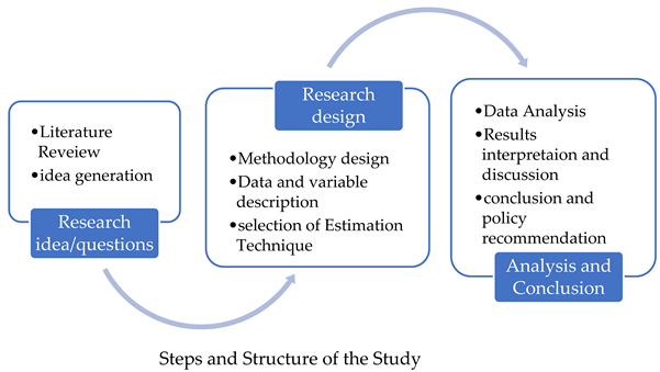
4. Steps Involved in Empirical Estimation of the STIRPAT Model

This study estimates the STIRPAT model by following four steps, namely, the cross-section dependence test, unit root test, co-integration test, and cross-sectional autoregressive distributive lag model. The cross-section dependence test is used to check whether any shock in one country will have an impact on other cross-sections or not. If cross-section dependence exists, the second-generation unit root test is used to test the stationarity of the series. Moreover, if the variables are stationary in a mixed order, a co-integration test is used to find the long-term co-integration among the modeled series. In addition, the augmented mean group (AMG) estimator is used to produce the long-term estimates. A methodological flowchart of this study is presented in Figure 3. It is worth mentioning that we transformed all the variables into their natural logarithmic forms to obtain more accurate results.

4.1. Cross-Sectional Dependence

Checking for cross-sectional dependence is necessary to obtain reliable results in panel data analysis [47]. Cross-sectional dependence might be caused by geographic location and interactions of socioeconomic networks within the cross-section [48]. Cross-sectional dependency refers to a situation where one unit within the panel experiences a shock or change; it can affect the other units as well. This study utilized the Pesaran CD test to check for the existence of cross-sectional dependence in the panel series based on following Pesaran CD equation.
CD = 2 T N ( N 1 ) i = 1 N 1 j = i + 1 N ρ i j
The Pesaran CD test assumes the null hypothesis that no cross-sectional dependence exists. Moreover, for fixed values of N (cross-sections) and T (time), the CD statistics have a mean of exactly zero for homogeneous/heterogeneous dynamic models and even for non-stationary models.

4.2. Second-Generation Unit Root Test

First-generation unit root tests such as those by Levin and Lin [49]; Hadri [50]; and Maddala and Wu [51] become inefficient when cross-sectional dependence exists in panel data. So, in the presence of cross-sectional dependence, second-generation unit root tests such as CADF and CIPS become necessary. These second-generation tests are designed to control cross-sectional dependency and produce more accurate results in the presence of correlated errors across panel units. Thus, the choice between first- and second-generation unit root tests depends crucially on whether cross-sectional dependency is present in the panel data being analyzed or not. The CADF test is a second-generation unit root test; it produces strong results when the period is greater than the cross-section. It was developed by Pesaran [52] and uses the Monte Carlo simulation method to calculate the critical values. Moreover, the CADF test is used to test unit roots for every unit-forming panel and for the panel itself. The CADF statistics are based on the following equation:
Y i t   = i   + b i   Y i , t 1   + j = 1 p i c i j   Y i , t 1   + d i t + h i   Y t 1 + j = 0 p i σ i j   Δ Y t 1   + i , t
This equation assumes the null hypothesis that the series has a unit root. i   indicates a constant, i , t is an error term, t is a trend, Y t 1   is the lag of the difference, and Y i t   is the one-term lag of Yt.
Similarly, the CIPS unit root test is an augmented form of the IPS unit root test. It includes cross-sectional averages of the series under consideration and helps to account for potential cross-sectional dependence among the units in the panel. The statistics of the CIPS test are based on the following equation,
CIPS = i 1 N t = 1 T p i t / T / N
where T is time and N is the cross-section, while p i t indicates the estimated autocorrelation of Y i t   .

4.3. Panel Co-Integration Tests

Due to cross-sectional dependence, traditional co-integration tests like those by Kao [53] and Pedroni [54] may produce biased results. So, to obtain unbiased and robust estimates, this study adopted the Westerlund [55] panel error correction cointegration test to find the long-term relationships among the modeled variables

Westerlund Co-Integration Test

The Westerlund error-correction-based co-integration test was developed by Westerlund [55]; the test is good and efficient in cases of the existence and non-existence of cross-sectional dependence. Moreover, this test produces reliable results even in small samples. The Westerlund panel produces model statistics based on panel-specific AR and the same AR based on the following equations.
VR = i = 1 N t = 1 T E i t ^ 2 R i ^ 1
VR = i = 1 N t = 1 T E i t ^ 2 ( i = 1 N R i ^ ) 1

4.4. Panel Long-Term Parameter Estimates

After the confirmation of long-term co-integration, this study employed a dynamic common correlated model to estimate the long-term estimates.

4.4.1. Augmented Mean Group (AMG) Estimator

Traditional panel data techniques are unable to produce reliable long-term estimates in the presence of cross-sectional dependence and slope heterogeneity, as shown by Wang and Dong [56]. However, second-generation panel data methodologies like the augmented mean group (AMG) estimation technique developed by Eberhardt and Bond [57] and Eberhardt and Teal [58] are appropriate for producing reliable and robust estimators in the presence of cross-sectional dependence and slope heterogeneity. The AMG technique utilizes a common dynamic effect coefficient to address CSD. The AMG technique is performed by following two steps; in the first step, estimators are obtained based on the following equation:
Y i t = α i + β i X i t + δ i f i + t 2 T π i   D i   + i
In the second stage, the AMG estimators are based on the following equation:
β A M G ^ N   i 1 N β i ^
α i is a constant term, i is an error term, Y i t   and X i t   are the dependent and independent variables, is the initial difference operator, f i is a common latent component with a heterogeneous slope factor, π i represent time dummy coefficients, and β A M G ^ is the group mean estimator.

4.4.2. Error Correction Model for Short-Term Estimates

This study also estimated the short-term coefficients/elasticity of the decarbonization variable concerning changes in P, A, REC, REP, and FD. This study utilized the ECM to calculate the short-term estimates of these short-term impacts, as earlier utilized by Mimi [59]. This study estimated the short-term estimates by using the following ECM equation.
Ln CBCO 2 = a + γ 1 ( Ln   P i t ) + γ 2 ( ( Ln   A i t ) + γ 3 ( ( Ln   R E C i t ) + γ 4 ( ( Ln   F F E C i t ) + γ 5 ECM + e i
Ln PBCO 2 = a + σ 1   ( ( Ln   P i t ) + σ 2   ( Ln   A i t ) + σ 3   ( Ln   R E P i t ) + σ 4   ( Ln   F F E C i t ) +   σ 5   ECM + e i
Ln CO 2 = a + φ 1   ( Ln   P i t ) + φ 2   ( Ln   A i t ) + φ 3   ( Ln   R E C i t   ) + φ 4   ( Ln   R E P i t ) + φ 5   ( Ln   F F E C i t ) +   φ 6   ECM +   e i
Ln CI = a + ψ 1   ( Ln   P i t ) + ψ 2   ( Ln   A i t ) + ψ 3   ( Ln   R E C i t   ) + ψ 4 ( Ln   R E P i t   ) + ψ 5 ( Ln   F F E C i t   ) +   ψ 6 E C M   + e i
Ln CIOE = a + π 1   ( Ln   P i t ) + π 2   ( Ln   A i t ) + π 3   ( Ln   R E C i t   ) + π 4   ( Ln   F F C i t   ) + π 5   ( Ln   F F E C i t   ) + π 6   ECM + e i
γ 1 , 4 , σ 1 , 4 , φ 1 , 5 , ψ 1 , ψ 5 , and π 1 , 5 , while the e i terms are error terms. Similarly, γ 5 , σ 5 , φ 6 , ψ 6 , and π 6 are error correction terms.

4.5. Dumitrescu–Hurlin (D-H) Panel Non-Causality Test

After investigating the long-term estimates, this study utilized the D-H panel non-causality test developed by Dumitrescu and Hurlin [60] because the traditional causality test, the Engle–Granger causality, is unable to account for slope heterogeneity. The D-H panel non-causality test accounts for slope heterogeneity and CSD and produces reliable and efficient results. The D-H test is a robust causality test based on the individual non-causality Granger [61] and Wald test statistics estimated through averaging across individual cross-sections. The D-H test estimates panel non-causality against the null hypothesis, i.e., there is no causality among the modeled variables, by using the following equation:
Y i t = i + j = 1 j δ   Y i , t j ) + j = 0 j η   X i ( t 1 )   + i , t
X and Y are observable variables, while δ and η are autoregressive coefficients that are subject to fluctuation across each cross-section. Moreover, this study estimated the Wald statistics based on the following equation:
W N , T ^ N 1   i 1 N W i , t ^
W N , T ^ is used to represent the individual Wald test statistics for all individual cross-sections. A list of abbreviations is also provided in Appendix A (see Table A6).

5. Empirical Analysis for Panel Data

In the first step, this study checked for CSD through the Pesaran CD test, and the results of the Pesaran cross-sectional dependence are reported in Table 3, which shows that for all series, the p-value of the CD test was less than the 0.05% level of significance, so the null hypothesis, i.e., there is cross-sectional independence, is rejected. Thus, the CD statistics ensure that cross-sectional dependence exists in all series across the cross-sections. Therefore, in the second step, this study employed the second-generation unit root test, the cross-sectionally augmented Im–Pesaran–Shin (CIPS) test, and the cross-sectional augmented Dickey–Fuller (CADF) unit root test, which produce reliable results in the presence of CSD. The results of the CIPS and CADAF tests are reported in Table 3.
The results indicate that carbon intensity and FD were stationary at a level, while all the other variables, i.e., production-based carbon emissions, consumption-based carbon emissions, carbon dioxide emissions, carbon intensity of electricity, renewable energy consumption, renewable energy production, fossil fuel consumption, GDP, and URB, were stationary at the first difference.
In the third step, this study employed the slope homogeneity test and the Westerlund co-integration, and the results are reported in Table 4. The results of the slope homogeneity test state that slopes were heterogeneous across the cross-sections and the results of the Westerlund co-integration revealed that long-term co-integration existed in all five models at the 10% level of significance.
After the confirmation of long-term co-integration in the five models, in the fourth step, this study employed the augmented mean group technique to estimate long-term estimators for the five models, while the ARDL error correction model was used to produce the error correction term and short-term estimates. The results of the AMG- and ARDL-based error correction models are reported in Table 5, Table 6, Table 7, Table 8 and Table 9. In the following section, this study aims to present and interpret the results model-wise.
Leading green economies are greatly committed to international agreements like the Paris Agreement, which sets targets for reducing greenhouse gas emissions. Leading green economies exert significant influence in global politics through the successful demonstration of decarbonization strategies, which can encourage other nations to follow suit and collaborate on global environmental goals. Thus, to check to what extent leading green economies are successful in their aim, this study investigated the key determinant of decarbonization in leading green economies. The results of the AMG test (long-term estimates) for the panel and individual cross-sections are reported in Table 5.
In model 1, the results indicated that fossil fuel energy consumption had a positive and significant impact on production-based CO2 emissions in Canada (β = 1.65 *). Our results were consistent with Erdoğan et al., [62] who reported that although Canada is trying to transform its energy production process, it still heavily relies on fossil fuels for electricity generation, heating, transportation, and industrial processes [63]. Moreover, despite having substantial hydroelectric power, fossil fuels still play a key role in electricity generation, especially in provinces in Canada without abundant hydro resources.
Similarly, renewable energy production significantly and negatively affected PBCO2 in Germany (β = −0.29 *), Canada (β = −0.15)*, Poland (β = −0.13 **), and Sweden (β = −0.07 *) in the long-term results. In addition, economic prosperity (GDP) significantly and positively affected PBCO2 emissions in all countries (β = 0.74 *; β = 1.09 *; β = 0.66 *; β = 0.73 *), except for Poland. Moreover, population positively and significantly affected PBCO2 in a panel of the green leaders group and in all individual cross-sections (β = 0.07 *; β = 0.11 *; β = 0.12 *; β = 0.08 *; β = 0.05 *), except for Denmark, where population and PBCO2 had a negative and significant association in the long-term period (β = −0.04 *).
Furthermore, the ARDL-based ECM estimates indicated that the model was stable; however, the speed of convergence varied across all cross-sections. The results indicated that in Denmark, the speed of convergence resulting from any shock was higher compared to the others; an almost 66% convergence took place in one year. Moreover, the results indicated that REP had a significant and negative impact on PBCO2 in the panel (β = −0.36 *), Germany (β = −0.37 *), and Sweden (β = −0.10 **) in the short-term period.
Moreover, the results of the full panel in model 1 indicated that REP negatively and significantly affected PBCO2 in the long-term (β = −0.15 *) as well as in the short-term period (β = −0.36 *), while GDP and urban population had a significant and positive impact on PBCO2 emissions in the long-term period (β = 0.74 *; β = 0.07 *) as well as in the short-term period. Our results implying that REP significantly increases decarbonization by lowering PBCO2 emissions is consistent with [62,63]. According to Zhang and Li [8], as the production of energy from renewable sources like wind, solar, and hydro increases, it will directly replace traditional energy sources and fossil fuel power plants in industries. So, this transition from coal, oil, and gas heating to electric heating will cause a significant reduction in CO2 emissions from production processes. Furthermore, a higher share of renewable energy in the electricity network means that all electricity-consuming production activities become greener as renewable energy diminishes carbon emissions [64].
In model 2, this study estimated the long-term estimates of key impact factors on consumption-based CO2 emissions. The results are reported in Table 6. The results indicated that FFEC had a positive and significant long-term association with CBCO2 emissions in Germany (β = 0.46 *), Denmark (β = 1.34 *), and Sweden (β = 1.80 *).
In addition, the results indicated that REC had a negative and significant long-term association with CBCO2 emissions in Denmark (β = −0.64 *), Poland (β = −0.24 *), and Sweden (β = −0.24 *). Furthermore, the results indicated that GDP had a positive and significant long-term association with CBCO2 emissions in Germany (β = 0.82 *), Poland (β = 0.63 *), and Sweden (β = 0.46 *), while it had a negative and significant long-term association with CBCO2 emissions in Denmark (β = −0.64 *). Similarly, population growth had a positive and significant impact on CBCO2 emissions in Denmark (β = 0.08 *) and a positive and significant impact on CBCO2 emissions in Germany (β = −0.09 **). In terms of the ARDL-based ECM (short-term estimates), the results shown in the lower part of Table 7 indicate that model 2 was stable and converged to the equilibrium growth path in the panel as well as in all cross-sections. The speed of the convergence was 24%, 27%, 25%, 33%, 26%, and 69%, respectively.
The result of the full panel in model 2 indicated that REC significantly lowered CBCO2 emissions and enhanced the decarbonization process in the leading green economies (β = −0.32 *). Our findings coincide with the existing literature [63,65] that has documented that renewable energy consumption helps to achieve carbon neutrality. The consumption of renewable energy from sources such as wind, solar, and hydro instead of fossil fuels will tend to reduce CO2 emissions from energy use [66]. Similarly, the utilization of electric vehicles and heating and cooling systems powered by renewable energy will further boost the process of decarbonization by lowering CO2 emissions from the consumption of goods and services.
In model 3, this study estimated the long-term estimates of the key impact factors on CO2 emissions, and the results are reported in Table 7. The results indicated that FFEC had a positive and significant long-term association with CO2 emissions in Germany (β = 2.43 *) and Poland (β = 0.245 *).
In addition, the results indicated that REP had a negative and significant long-term association with CO2 emissions in Denmark (β = −0.81 *) and Poland (β = −0.458 *). The results also indicated that REC had a negative and significant long-term association with CO2 emissions in Denmark (β = −0.39 *) and Sweden (β = −1.47 *).
Furthermore, the results indicated that GDP had a positive and significant long-term association with CO2 emissions in Germany (β = 0.64 *) and Denmark (β = 0.75 *). Similarly, population growth had a negative and significant impact on CO2 emissions in Denmark (β = −0.04 *) and Sweden (β = −0.72 *). In terms of the ARDL-based ECM (short-term estimates), the results in the lower part of Table 8 indicate that model 3 was stable and converged to the equilibrium growth path in the panel as well as in all cross-sections. The speed of the convergence was 16%, 15%, 34%, 32%, 45%, and 13%, respectively.
The results of the impact of FFEC, REP, REC, GDP, and urban POP on CO2 emissions in the full panel of the leading green economies are reported in Table 7 for model 3. The results are very interesting and reinforce our previous results of model 1 and model 2. The results showed that fossil fuel use had an insignificant relationship with CO2 emissions (β = −1.21). Our results indicated that the leading green economies have significantly lowered their reliance on fossil fuel for energy production, so the contribution of fossil fuels to CO2 emissions was minor and insignificant [67]. In the leading green economies, a greater proportion of the energy mix comes from solar, wind, and hydro power, which produces little or no CO2 emissions. Moreover, it has been examined that in leading green economies, policies and strict regulations ensure keeping CO2 emissions at a minimum level, and they also use carbon capture and storage (CCS) technologies to capture CO2 emissions from fossil fuel power plants [68]. The results of the full panel in model 3 also indicated that renewable energy production and consumption significantly lowered CO2 emission and enhanced the decarbonization process in the leading green economies. The results of model 3 were similar to those of model 1 and model 2, as [34] showed that the transition towards cleaner energy sources is significantly associated with reductions in CO2 emissions, and [35] stated that the transition towards renewable energy consumption and production helps to curb CO2 emissions and to achieve decarbonization targets.
In model 4, this study estimated the long-term estimates of key impact factors on CI, and the results are reported in Table 8. The results indicated that FFEC had a positive and significant long-term association with CI in Poland (β = 0.21 *) and Sweden (β = 3.09 *). In addition, the results indicated that REP and REC had a negative and significant long-term association with CI in Denmark (β = −0.53 *; β = −0.37 *), Poland (β = −0.29 *; β = −0.11 *), and Sweden (β = −0.22 *; β = −0.12 *). Furthermore, the results indicated that GDP had a positive and significant long-term association with CI in Canada (β = 0.40 *), while population growth had a negative and significant impact on CI in Germany (β = −0.19 *), Canada (β = 0.11 *), and Denmark (β = −0.05 *). In terms of the ARDL-based ECM (short-term estimates), the results in the lower part of Table 9 indicate that model 3 was stable and converged to the equilibrium growth path in the panel as well as in all cross-sections. The speed of the convergence was 25%, 62%, 27%, 28%, 19%, and 30%, respectively.
The overall results for the full panel in model 4 state that FFEC, REP, and REC had insignificant associations with carbon intensity (CI), the amount of carbon dioxide (CO2) emissions produced per unit of a specific activity. The reason behind this relationship is the high utilization of renewable energy sources in these countries. This means that even if some fossil fuels are used in specific instances (e.g., backup power or in sectors hard to electrify), their overall contribution to carbon intensity remains minimal due to the predominance of low-carbon or carbon-neutral energy sources. Similarly, the leading green economies have already achieved a high penetration of renewable energy in their energy mix, which has significantly reduced the carbon intensity to a minimum level. Thus, further increases in renewable energy consumption may have a minimal impact on reducing overall carbon intensity. The initial shift to renewables has already significantly lowered their carbon intensity, making additional reductions more challenging and less impactful relative to economies with higher fossil fuel dependence.
In model 5, this study estimated the long-term estimates of the key impact factors of CIOE, and the results are reported in Table 9. The results indicated that FFEC had a positive and significant long-term association with CIOE in Germany (β = 1.75 *) and Canada (β = 4.05 *).
In addition, the results indicated that REP and REC had a negative and significant long-term association with CIOE in Germany (β = −1.13 *; β = −0.47 *) and Poland (β = −1.13 *; β = −0.53 *), and REC also had a significant and negative impact on CIOE in Denmark (β = −1.10 *).
Furthermore, the results indicated that GDP and population had insignificant impacts on CIOE in all cross-sections. In terms of the ARDL-based ECM (short-term estimates), the results in the lower part of Table 9 indicate that model 3 was stable and converged to the equilibrium growth path in the panel as well as in all cross-sections. The speed of the convergence was 32%, 13%, 47%, 48%, 57%, and 22%, respectively.
The results indicated that REP and REC had a negative and significant long-term association with CIOE in the full panel of the leading green economies (β = −0.04 *; β = −0.41 *). In other words, increased REC and REP values promote decarbonization by lowering CIOE, in line with [69,70]. Similarly, hydro and geothermal power also lower CIOE because they produce electricity with minimal or zero direct emissions.

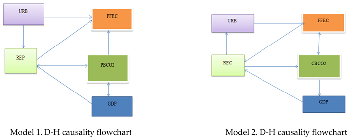
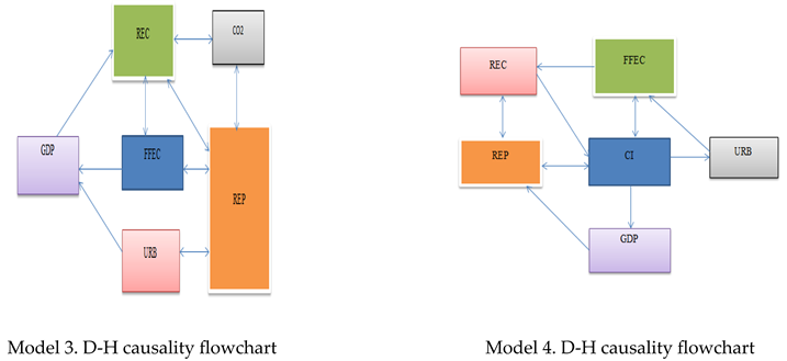
Dumitrescu–Hurlin (D-H) Panel Causality

After investigating the long-term estimates of the five developed models, it was imperative to determine the direction of the causality relationship among the variables [71,72]. For this purpose, this study utilized the Dumitrescu and Hurlin [60] non-causality tests and obtained evidence of bidirectional, unidirectional, and neutral relationships among the defined variables. The detailed results are reported in Appendix A (see Table A1, Table A2, Table A3, Table A4 and Table A5). However, a graphical representation of the five models based on Table A1, Table A2, Table A3, Table A4 and Table A5 are presented in following figure with the names model 1, 2, 3, 4, and 5. Energies 17 04600 i003
The results of model 1 indicate that there was a bidirectional causality between production-base CO2 emissions and GDP, while there was a unidirectional causality between production-based CO2 emissions and FFEC; GDP and renewable energy production; urban population and renewable energy production; urban population and FFEC; and GDP and REP. Similarly, model 2 indicated that there was a bidirectional causality between CBCO2 and FFEC, while there was a unidirectional causality between consumption-based CO2 emissions and GDP; GDP and renewable energy consumption; REC and CBCO2; REC and urban population; and REC and FFEC.Energies 17 04600 i004
The causality relationship flowchart of model 3 is reported, and the results indicated that there was a bidirectional causality between REC and FFEC; REP and FFEC; REC and CO2; REP and CO2; REC and REP; and REP and urban population. Moreover, there was a unidirectional causality between urban population and GDP; GDP and REC; and FFEC and GDP. Similarly, model 4 indicated that there was a bidirectional causality between REP and REC; REP and CI; and FFEC and CI, while there was a unidirectional causality between GDP and REP; FFEC and REC; urban population and FFEC; REC and CI; and CI and GDP. Similarly, model 5 indicated that there was no bidirectional causality in the model. However, there was a unidirectional causality between REP and REC; CIOE and REP; CIOE and REC; CIOE and FFEC; GDP and FFEC; FFEC and REC; and urban population and FFEC. Energies 17 04600 i005

6. Conclusions

This study investigated the impact of fossil fuel energy consumption (FFEC), renewable energy production (REP) and renewable energy consumption (REC), urban population, and economic affluence on decarbonization in the context of leading green economies from 2000 to 2023. This study utilized five measurements to measure decarbonization, including production-based CO2 emissions (PBCO2), consumption-based CO2 emissions (CBCO2), CO2 emissions, carbon intensity (CI), and carbon intensity of electricity (CIOE). Thus, this study developed five models to assess the impact of key impact factors, namely, fossil fuel energy consumption, renewable energy production and renewable energy consumption, urban population, and economic affluence on decarbonization. This study utilized the augmented mean group (AMG) technique to assess the long-term estimates among the modeled variables. The findings are described model-wise as follows.
The findings of model 1 indicate, in the full panel, that REP significantly lowered PBCO2 and enhanced the decarbonization process in the leading green economies, while economic affluence and urban population significantly increased PBCO2 and hindered the process of decarbonization in the leading green economies. Similar results were obtained in Germany, Canada, Poland, and Sweden. However, in Denmark, REP increased PBCO2 emissions and hindered the decarbonization process, while urban population significantly lowered PBCO2 emissions and facilitated the process of decarbonization.
The findings of model 2 indicate that, in the full panel, REC significantly lowered CBCO2 emissions and enhanced the decarbonization process, while economic affluence significantly lowered decarbonization by increasing CBCO2 emissions. Similarly, the findings of model 2 indicate that in Germany, FFEC decreased decarbonization by increasing CBCO2 emissions, while urban population enhanced decarbonization by reducing CBCO2 emissions. In Denmark. FFEC and urban population significantly lowered decarbonization by increasing CBCO2 emissions, while REC and economic affluence significantly enhanced the decarbonization process by decreasing CBCO2 emissions. Furthermore, in Poland, REC significantly improved decarbonization, and economic affluence decreased the decarbonization process. Similar results were found in Sweden.
The findings of model 3 indicate that, in the full panel, REP and REC significantly lowered CO2 emissions and increased the decarbonization process. In Germany, FFEC and economic prosperity significantly increased CO2 emissions and lowered decarbonization. In Denmark, REP, REC, and urban population significantly increased the decarbonization process by lowering CO2 emissions, while economic prosperity increased CO2 emissions and lowered decarbonization. Furthermore, the results indicate that in Poland, FFEC lowered decarbonization, and REP enhanced the decarbonization process, while in Sweden, REC and urban population significantly enhanced decarbonization by lowering CO2 emissions.
The findings of model 4 indicate that, in the full panel, only urban population significantly enhanced decarbonization by lowering carbon intensity, while in Germany, urban population increased carbon intensity and lowered decarbonization. In Canada, economic affluence increased CI and lowered decarbonization, while urban population decreased CI and enhanced the decarbonization process. The results also indicate that in Denmark, REC, REP, and urban population significantly lowered CI and enhanced decarbonization. Similarly, in Poland, FFEC decreased decarbonization, and REP and REC significantly lowered CI and enhanced decarbonization. In Sweden, FFEC significantly lowered decarbonization by increasing CI, and REC enhanced decarbonization in Sweden by decreasing CI.
The findings of model 5 indicate that, in the full panel, REP and REC significantly lowered CIOE and enhanced decarbonization, while in Germany, FFEC significantly lowered decarbonization. Similarly, REP and REC significantly enhanced decarbonization by decreasing CIOE. in Canada, FFEC significantly lowered the decarbonization process, while in Denmark, REC significantly improved the decarbonization process. In Poland, REP and REC significantly enhanced the decarbonization process.

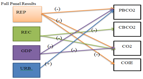
6.1. Graphical Presentation of Results and Policy Suggestions

Results for Full Panel

The flow diagram of the full-panel results indicates that REP significantly and negatively affected PBCO2, CO2, and COIE. Similarly, REC negatively affected CBCO2 and CO2 emissions in the leading green economies. GDP negatively and significantly affected PBCO2 emissions and CO2 emissions, while urban population affected PBCO2 emissions positively and significantly in the leading green economies. The findings suggest that renewable energy consumption and renewable energy production should be promoted to achieve a zero-carbon economy. Moreover, this study suggests that planned urbanization is required to lower PBCO2 emissions and to increase the process of decarbonization. Energies 17 04600 i006
Based on the findings of this study, policymakers in leading green economies should focus on comprehensive strategies to reduce fossil fuel energy consumption (FFEC) and promote renewable energy production (REP) and consumption (REC) to enhance decarbonization efforts. To reduce FFEC, policymakers should implement regulations such as carbon taxes to make fossil fuel use more expensive and less attractive, thereby incentivizing businesses and consumers to shift towards cleaner energy sources. They should also phase out subsidies for fossil fuel industries and redirect those funds to support renewable energy projects, ensuring a financial shift towards greener energy. Setting stringent emissions reduction targets and implementing cap-and-trade systems to limit the total amount of CO2 emissions are crucial steps in this transition. Promoting REP and REC requires providing financial incentives like grants, tax credits, and low-interest loans for the development and installation of renewable energy infrastructure, including solar farms and wind turbines. Investing in renewable energy infrastructure, such as smart grids and energy storage systems, will ensure a stable and efficient energy supply, making renewable energy more viable. Additionally, implementing feed-in tariffs to guarantee that renewable energy producers receive a fixed price for the energy they generate can encourage more investment in this sector.
In country-specific contexts, we suggest that Germany should prioritize environmentally friendly development projects, including promoting green urban policies like green urban planning, sustainable transportation solutions, and energy-efficient building codes. Public awareness campaigns to encourage pro-environmental behaviors among the urban population are also essential. In Denmark, policymakers should continue supporting renewable energy initiatives and consider policies that reduce urban CO2 emissions further, such as expanding public transportation options and promoting bicycle use through improved infrastructure. Poland and Sweden should focus on increasing the share of renewable energy in their energy mix and improving urban planning to integrate more green spaces and energy-efficient public infrastructure.
Limitations and Future Research Direction:
This study included only five countries, namely, Germany, Canada, Sweden, Denmark, and Poland due to data availability. Moreover, this study did not analyze the impact of global events like COVID-19 on decarbonization. Future studies can incorporate global events into their empirical models. Furthermore, varying levels of technology adoption and innovation can affect the decarbonization process, so future studies can investigate that how different levels of technology adoption can affect the decarbonization process.

Author Contributions

Conceptualization, S.K. and F.A.; data curation, A.P. and F.A.; formal analysis, S.K. and F.A.; methodology, S.K. and F.A.; writing—original draft, S.K., F.A. and F.M.N.; writing—review and editing, F.M.N. All authors have read and agreed to the published version of the manuscript.

Funding

This research received no external funding.

Data Availability Statement

Data is available online.

Conflicts of Interest

The authors declare no conflicts of interest.

Appendix A

Table A1. Pairwise Dumitrescu–Hurlin panel causality tests; model 1.
Null HypothesisW-Stat.Zbar-Stat.Prob.Decision
LOGFFEC LOGPBCO23.611.130.26No causality
LOGPBCO2 LOGFFEC16.5412.080.00PBCO2 causes FFEC
LOGREP LOGPBCO22.710.360.72No causality
LOGPBCO2 LOGREP4.271.680.09Bidirectional causality
LOGGDP LOGPBCO25.602.810.01
LOGPBCO2 LOGGDP16.9312.400.00Bidirectional causality
URB LOGPBCO25.392.630.01
LOGPBCO2 URB1.64−0.550.58No causality
LOGREP LOGFFEC20.7915.670.00REP causes FFEC
LOGFFEC LOGREP3.270.830.41No causality
LOGGDP LOGFFEC7.964.800.00No causality
LOGFFEC LOGGDP2.960.580.57No causality
URB LOGFFEC6.403.480.00URB causes FFEC
LOGFFEC URB2.05−0.200.84No causality
LOGGDP LOGREP5.032.320.02GDP causes REP
LOGREP LOGGDP2.530.210.83No causality
URB LOGREP4.972.270.02URB causes REP
Table A2. Pairwise Dumitrescu–Hurlin panel causality tests; model 2.
Null HypothesisW-Stat.Zbar-Stat.Prob.Decision
LOGFFEC LOGCBCO24.892.210.03Bidirectional causality
LOGCBCO2 LOGFFEC4.992.290.02
LOGREC LOGCBCO24.972.280.02REC → CBCO2
LOGCBCO2 LOGREC10.486.940.00No causality
LOGGDP LOGCBCO28.555.310.00No causality
LOGCBCO2 LOGGDP17.9713.290.00CBCO2 → GDP
URB LOGCBCO28.415.190.00No causality
LOGCBCO2 URB3.410.950.34No causality
LOGREC LOGFFEC2.880.510.61No causality
LOGFFEC LOGREC6.443.520.00FFEC → REC
URB LOGFFEC6.403.480.00URB → FFEC
LOGFFEC URB2.05−0.200.84No causality
LOGGDP LOGREC8.865.570.00No causality
LOGREC LOGGDP2.04−0.200.84No causality
URB LOGREC8.665.400.00No causality
LOGREC URB5.402.640.01REC → URB
Table A3. Pairwise Dumitrescu–Hurlin panel causality tests; model 3.
Null HypothesisW-Stat.Zbar-Stat.Prob.Decision
LOGFFEC LOGCO24.374.200.00No causality
LOGCO2 ↛ LOGFFEC4.574.460.00No causality
LOGREC ↛ LOGCO22.221.430.15No causality
LOGCO2 ↛ LOGREC4.484.340.00No causality
LOGREP ↛ LOGCO27.868.700.00Bidirectional causality
LOGCO2 ↛ LOGREP3.222.710.01
LOGGDP ↛ LOGCO27.167.810.00No causality
LOGCO2 ↛ LOGGDP2.371.620.11No causality
URB ↛ LOGCO25.335.440.00No causality
LOGCO2 ↛ URB1.210.110.91No causality
LOGREC ↛ LOGFFEC1.710.770.44No causality
LOGFFEC ↛ LOGREC3.953.660.00Bidirectional causality
LOGREP ↛ LOGFFEC10.4712.080.00
LOGFFEC ↛ LOGREP2.431.690.09Bidirectional causality
LOGGDP ↛ LOGFFEC8.279.240.00
LOGFFEC ↛ LOGGDP2.732.080.04FFEC → GDP
URB ↛ LOGFFEC5.605.790.00No causality
LOGFFEC ↛ URB4.774.710.00No causality
LOGREP ↛ LOGREC18.8322.870.00Bidirectional causality
LOGREC ↛ LOGREP3.893.580.00
LOGGDP ↛ LOGREC4.123.870.00GDP → REC
URB ↛ LOGREP8.089.000.00Bidirectional causality
LOGREP ↛ URB19.5523.810.00
URB ↛ LOGGDP2.471.750.08URB → GDP
LOGGDP ↛ URB6.296.680.00No causality
Table A4. Pairwise Dumitrescu–Hurlin panel causality tests; model 4.
Null HypothesisW-Stat.Zbar-Stat.Prob.Decision
LOGFFEC ↛ LOGCI6.643.690.00Bidirectional causality
LOGCI ↛ LOGFFEC5.222.480.01
LOGREC ↛ LOGCI5.402.640.01REC → CI
LOGCI ↛ LOGREC7.364.300.00No causality
LOGREP ↛ LOGCI6.863.880.00Bidirectional causality
LOGCI ↛ LOGREP5.702.890.00
LOGGDP ↛ LOGCI4.181.610.11No causality
LOGCI ↛ LOGGDP5.752.930.00CI → GDP
URB ↛ LOGCI4.111.550.12No causality
LOGCI ↛ URB6.783.810.00CI →URB
LOGFFEC ↛ LOGREC6.443.520.00FFEC → REC
LOGREP ↛ LOGFFEC20.7915.670.00
LOGFFEC ↛ LOGREP3.270.830.41No causality
LOGGDP ↛ LOGFFEC7.964.800.00No causality
LOGFFEC ↛ LOGGDP2.960.580.57No causality
URB ↛ LOGFFEC6.403.480.00URB → FFEC
LOGFFEC ↛ URB2.05−0.200.84No causality
LOGREP ↛ LOGREC56.1345.620.00Bidirectional causality
LOGREC ↛ LOGREP5.913.070.00
LOGGDP ↛ LOGREC8.865.570.00No causality
LOGREC ↛ LOGGDP2.04−0.200.84No causality
LOGREC ↛ URB5.402.640.01REC → URB
LOGGDP ↛ LOGREP5.032.320.02GDP → REP
Table A5. Pairwise Dumitrescu–Hurlin panel causality tests; model 5.
DV = CIOE
Null HypothesisW-Stat.Zbar-Stat.Prob.Decision
LOGFFEC ↛ LOGCIOE5.641.300.19No causality
LOGCIOE ↛ LOGFFEC9.173.480.00CIOE → FFEC
LOGREC ↛ LOGCIOE5.941.480.14No causality
LOGCIOE ↛ LOGREC8.152.850.00CIOE → REC
LOGREP ↛ LOGCIOE2.65−0.550.58No causality
LOGCIOE ↛ LOGREP6.741.980.05CIOE → REP
LOGGDP ↛ LOGCIOE3.890.210.83No causality
LOGCIOE ↛ LOGGDP10.464.280.00No causality
URB ↛ LOGCIOE4.240.430.67No causality
LOGCIOE ↛ URB2.73−0.510.61No causality
LOGFFEC ↛ LOGREC7.022.150.03FFEC → REC
LOGREP ↛ LOGFFEC17.008.340.00REP → FFEC
LOGFFEC ↛ LOGREP2.71−0.520.60No causality
LOGGDP ↛ LOGFFEC8.473.050.00GDP → FFEC
LOGFFEC ↛ LOGGDP4.060.320.75No causality
URB ↛ LOGFFEC7.372.370.02URB → FFEC
LOGFFEC ↛ URB4.880.830.41No causality
LOGREP ↛ LOGREC46.7826.780.00REP → REC
LOGREC ↛ LOGREP4.950.870.38No causality
LOGGDP ↛ LOGREC8.953.350.00GDP → REC
LOGREC ↛ URB9.033.400.00REC → URB
URB ↛ LOGREP6.701.950.05URB → REP
Table A6. List of abbreviations.
VariableNotationTestsNotation
Carbon EmissionsCO2Augmented mean group AMG
Consumption-Based Carbon EmissionsCBCO2Greenhouse gases GHGs
Production Based Carbon EmissionsPBCO2Conference of the PartiesCOP
Carbon IntensityCIThe Organization for Economic Cooperation and Development OECD
Carbon Intensity of ElectricityCIOEDumitrescu–Hurlin D-H
Fossil Fuel Energy ConsumptionFFECCross-sectional dependanceCSD
Renewable Energy ConsumptionRECCross-sectional augmented Dickey–FullerCADF
Renewable Energy ProductionREPCross-sectionally augmented Im–Pesaran–ShinCIPS
PopulationURBPesaran cross-sectional dependancePesaran CD
Gross Domestic ProductGDPStochastic Regression on Population, Affluence, and TechnologySTIRPAT

References

  1. Wang, J.; Azam, W. Natural resource scarcity, fossil fuel energy consumption, and total greenhouse gas emissions in top emitting countries. Geosci. Front. 2024, 15, 101757. [Google Scholar] [CrossRef]
  2. Dechamps, P. The IEA World Energy Outlook 2022—A brief analysis and implications. Eur. Energy Clim. J. 2023, 11, 100–103. [Google Scholar] [CrossRef]
  3. Gani, A. Fossil fuel energy and environmental performance in an extended STIRPAT model. J. Clean. Prod. 2021, 297, 126526. [Google Scholar] [CrossRef]
  4. de Coninck, H.; Revi, A.; Babiker, M.; Bertoldi, P.; Buckeridge, M.; Cartwright, A.; Dong, W.; Ford, J.; Fuss, S.; Hourcade, J.C.; et al. Strengthening and Implementing the Global Response; Energy (ENE) Risk & Resilience (RISK): Santa Ana, CA, USA, 2018. [Google Scholar]
  5. Bai, J.; Han, Z.; Rizvi, S.K.A.; Naqvi, B. Green trade or green technology? The way forward for G-7 economies to achieve COP 26 targets while making competing policy choices. Technol. Forecast. Soc. Chang. 2023, 191, 122477. [Google Scholar] [CrossRef]
  6. COP. United Nations Climate Change Conference. 2021. Available online: https://unfccc.int/conference/glasgow-climate-change-conference-october-november-2021 (accessed on 28 July 2024).
  7. Arora, P. COP28: Ambitions, realities, and future. Environ. Sustain. 2024, 7, 107–113. [Google Scholar] [CrossRef]
  8. Zhang, Y.; Li, L.; Sadiq, M.; Chien, F. The impact of non-renewable energy production and energy usage on carbon emissions: Evidence from China. Energy Environ. 2023, 35, 2248–2269. [Google Scholar] [CrossRef]
  9. Hassan, Q.; Viktor, P.; Al-Musawi, T.J.; Ali, B.M.; Algburi, S.; Alzoubi, H.M.; Al-Jiboory, A.K.; Sameen, A.Z.; Salman, H.M.; Jaszczur, M. The renewable energy role in the global energy Transformations. Renew. Energy Focus 2024, 48, 100545. [Google Scholar] [CrossRef]
  10. Abbas, S.; Kousar, S.; Pervaiz, A. Effects of energy consumption and ecological footprint on CO2 emissions: An empirical evidence from Pakistan. Environ. Dev. Sustain. 2021, 23, 13364–13381. [Google Scholar] [CrossRef]
  11. Yin, Z.; Lu, X.; Chen, S.; Wang, J.; Wang, J.; Urpelainen, J.; Fleming, R.M.; Wu, Y.; He, K. Implication of electrification and power decarbonization in low-carbon transition pathways for China, the U.S. and the EU. Renew. Sustain. Energy Rev. 2023, 183, 113493. [Google Scholar] [CrossRef]
  12. Schmidt, L.; Apergi, M.; Eicke, L.; Weko, S. Who believes in green growth? Strategic framing and technology leadership in the UNFCCC negotiations. Clim. Policy 2023, 24, 177–192. [Google Scholar] [CrossRef]
  13. Kartal, M.T.; Taşkın, D.; Shahbaz, M.; Kirikkaleli, D.; Kılıç Depren, S. Role of energy transition in easing energy security risk and decreasing CO2 emissions: Disaggregated level evidence from the USA by quantile-based models. J. Environ. Manag. 2024, 359, 120971. [Google Scholar] [CrossRef] [PubMed]
  14. Zeng, C.; Stringer, L.C.; Lv, T. The spatial spillover effect of fossil fuel energy trade on CO2 emissions. Energy 2021, 223, 120038. [Google Scholar] [CrossRef]
  15. Li, B.; Haneklaus, N. The role of renewable energy, fossil fuel consumption, urbanization and economic growth on CO2 emissions in China. Energy Rep. 2021, 7, 783–791. [Google Scholar] [CrossRef]
  16. Abbasi, K.R.; Shahbaz, M.; Zhang, J.; Irfan, M.; Alvarado, R. Analyze the environmental sustainability factors of China: The role of fossil fuel energy and renewable energy. Renew. Energy 2022, 187, 390–402. [Google Scholar] [CrossRef]
  17. Yi, S.; Abbasi, K.R.; Hussain, K.; Albaker, A.; Alvarado, R. Environmental concerns in the United States: Can renewable energy, fossil fuel energy, and natural resources depletion help? Gondwana Res. 2023, 117, 41–55. [Google Scholar] [CrossRef]
  18. Zimon, G.; Pattak, D.C.; Voumik, L.C.; Akter, S.; Kaya, F.; Walasek, R.; Kochański, K. The impact of fossil fuels, renewable energy, and nuclear energy on South Korea’s environment based on the STIRPAT model: ARDL, FMOLS, and CCR Approaches. Energies 2023, 16, 6198. [Google Scholar] [CrossRef]
  19. Bukhari, W.A.A.; Pervaiz, A.; Zafar, M.; Sadiq, M.; Bashir, M.F. Role of renewable and non-renewable energy consumption in environmental quality and their sub-sequent effects on average temperature: An assessment of sustainable development goals in South Korea. Environ. Sci. Pollut. Res. 2023, 30, 115360–115372. [Google Scholar] [CrossRef] [PubMed]
  20. Hou, H.; Lu, W.; Liu, B.; Hassanein, Z.; Mahmood, H.; Khalid, S. Exploring the role of fossil fuels and renewable energy in determining environmental sustainability: Evidence from OECD countries. Sustainability 2023, 15, 2048. [Google Scholar] [CrossRef]
  21. Madaleno, M.; Nogueira, M.C. How renewable energy and CO2 emissions contribute to economic growth, and sustaina-bility—An extensive analysis. Sustainability 2023, 15, 4089. [Google Scholar] [CrossRef]
  22. Ahmed, F.; Kousar, S.; Pervaiz, A.; Trinidad-Segovia, J.E.; Casado-Belmonte, M.d.P.; Ahmed, W. Role of green innovation, trade and energy to promote green economic growth: A case of South Asian Nations. Environ. Sci. Pollut. Res. 2021, 29, 6871–6885. [Google Scholar] [CrossRef]
  23. Omri, E.; Saadaoui, H. An empirical investigation of the relationships between nuclear energy, economic growth, trade openness, fossil fuels, and carbon emissions in France: Fresh evidence using asymmetric cointegration. Environ. Sci. Pollut. Res. 2022, 30, 13224–13245. [Google Scholar] [CrossRef] [PubMed]
  24. Dar, J.; Asif, M. Environmental feasibility of a gradual shift from fossil fuels to renewable energy in India: Evidence from multiple structural breaks cointegration. Renew. Energy 2023, 202, 589–601. [Google Scholar] [CrossRef]
  25. Zhao, C.; Wang, J.; Dong, K.; Wang, K. How does renewable energy encourage carbon unlocking? A global case for decarbonization. Resour. Policy 2023, 83, 103622. [Google Scholar] [CrossRef]
  26. Abban, O.J.; Xing, Y.H.; Nuta, A.C.; Rajaguru, G.; Acheampong, A.O.; Nuta, F.M. The road to decarbonization in Australia. A Morlet wavelet approach. J. Environ. Manag. 2024, 365, 121570. [Google Scholar] [CrossRef]
  27. Usman, O. Renewable energy and CO2 emissions in G7 countries: Does the level of expenditure on green energy technologies matter? Environ. Sci. Pollut. Res. 2023, 30, 26050–26062. [Google Scholar] [CrossRef]
  28. Osei Opoku, E.E.; Acheampong, A.O.; Dogah, K.E.; Koomson, I. Energy innovation investment and renewable energy in OECD countries. Energy Strategy Rev. 2024, 54, 101462. [Google Scholar] [CrossRef]
  29. Mirziyoyeva, Z.; Salahodjaev, R. Renewable energy, GDP and CO2 emissions in high-globalized countries. Front. Energy Res. 2023, 11, 1123269. [Google Scholar] [CrossRef]
  30. Apergis, N.; Kuziboev, B.; Abdullaev, I.; Rajabov, A. Investigating the association among CO2 emissions, renewable and non-renewable energy consumption in Uzbekistan: An ARDL approach. Environ. Sci. Pollut. Res. 2023, 30, 39666–39679. [Google Scholar] [CrossRef]
  31. Kuldasheva, Z.; Salahodjaev, R. Renewable energy and CO2 emissions: Evidence from rapidly urbanizing countries. J. Knowl. Econ. 2022, 14, 1077–1090. [Google Scholar] [CrossRef]
  32. Wang, H.; Wen, C.; Duan, L.; Li, X.; Liu, D.; Guo, W. Sustainable energy transition in cities: A deep statistical prediction model for renewable energy sources management for low-carbon urban development. Sustain. Cities Soc. 2024, 107, 105434. [Google Scholar] [CrossRef]
  33. Awosusi, A.A.; Ozdeser, H.; Seraj, M.; Abbas, S. Can green resource productivity, renewable energy, and economic globalization drive the pursuit of carbon neutrality in the top energy transition economies? Int. J. Sustain. Dev. World Ecol. 2023, 30, 745–759. [Google Scholar] [CrossRef]
  34. Zhao, C.; Wang, J.; Dong, K.; Wang, K. Is renewable energy technology innovation an excellent strategy for reducing climate risk? The case of China. Renew. Energy 2024, 223, 120042. [Google Scholar] [CrossRef]
  35. Malcher, X.; Gonzalez-Salazar, M. Strategies for decarbonizing European district heating: Evaluation of their effectiveness in Sweden, France, Germany, and Poland. Energy 2024, 306, 132457. [Google Scholar] [CrossRef]
  36. Kirikkaleli, D.; Awosusi, A.A.; Adebayo, T.S.; Otrakçı, C. Enhancing environmental quality in Portugal: Can CO2 intensity of GDP and renewable energy con-sumption be the solution? Environ. Sci. Pollut. Res. 2023, 30, 53796–53806. [Google Scholar] [CrossRef] [PubMed]
  37. Raihan, A.; Bari, A.M. Energy-economy-environment nexus in China: The role of renewable energies toward carbon neutrality. Innov. Green Dev. 2024, 3, 100139. [Google Scholar] [CrossRef]
  38. Ding, Q.; Khattak, S.I.; Ahmad, M. Towards sustainable production and consumption: Assessing the impact of energy productivity and eco-innovation on consumption-based carbon dioxide emissions (CCO2) in G-7 nations. Sustain. Prod. Consum. 2020, 27, 254–268. [Google Scholar] [CrossRef]
  39. Smil, V. World history and energy. Encycl. Energy 2004, 6, 549. [Google Scholar]
  40. Vinayak, A.K.; Gurumoorthy, A.V. Vaclav Smil’s Perspective on Fossil Fuels and Renewable Energy: A Review. Pet. Coal 2020, 62, 1231–1239. [Google Scholar]
  41. Smil, V. Energy Transitions: History, Requirements, Prospects; Praeger: Santa Barbara, CA, USA, 2010. [Google Scholar]
  42. Holdren, J. A brief history of IPAT. J. Popul. Sustain. 2018, 2, 66–74. [Google Scholar] [CrossRef]
  43. York, R.; Rosa, E.A.; Dietz, T. STIRPAT, IPAT and ImPACT: Analytic tools for unpacking the driving forces of environmental impacts. Ecol. Econ. 2003, 46, 351–365. [Google Scholar] [CrossRef]
  44. Du, Q.; Li, Z.; Du, M.; Yang, T. Government venture capital and innovation performance in alternative energy production: The moderating role of environmental regulation and capital market activity. Energy Econ. 2024, 129, 107196. [Google Scholar] [CrossRef]
  45. Shahbaz, M.; Papavassiliou, V.G.; Lahiani, A.; Roubaud, D. Are we moving towards decarbonisation of the global economy? Lessons from the distant past to the present. Int. J. Finance Econ. 2021, 28, 2620–2634. [Google Scholar] [CrossRef]
  46. Naveed, A.; Ahmad, N.; Aghdam, R.F.; Menegaki, A.N. What have we learned from Environmental Kuznets Curve hypothesis? A citation-based systematic literature review and content analysis. Energy Strat. Rev. 2022, 44, 100946. [Google Scholar] [CrossRef]
  47. Grossman, G.M.; Krueger, A.B. Economic growth and the environment. Q. J. Econ. 1995, 110, 353–377. [Google Scholar] [CrossRef]
  48. Chudik, A.; Pesaran, M.H. Large Panel Data Models with Cross-Sectional Dependence: A Survey. CAFE Research Paper No. 13.15. 2013. Available online: https://ssrn.com/abstract=2316333 (accessed on 28 July 2024).
  49. Levin, A.; Lin, C.-F.; Chu, C.-S.J. Unit root tests in panel data: Asymptotic and finite-sample properties. J. Econ. 2002, 108, 1–24. [Google Scholar] [CrossRef]
  50. Hadri, K. Testing for stationarity in heterogeneous panel data. Econ. J. 2000, 3, 148–161. [Google Scholar] [CrossRef]
  51. Maddala, G.S.; Wu, S. A comparative study of unit root tests with panel data and a new simple test. Oxf. Bull. Econ. Stat. 1999, 61, 631–652. [Google Scholar] [CrossRef]
  52. Pesaran, M.H. Estimation and Inference in Large Heterogenous Panels with Cross Section Dependence. Available at SSRN 385123. 2003. Available online: https://ssrn.com/abstract=385123 (accessed on 28 July 2024).
  53. Kao, C. Spurious regression and residual-based tests for cointegration in panel data. J. Econ. 1999, 90, 1–44. [Google Scholar] [CrossRef]
  54. Pedroni, P. Critical values for cointegration tests in heterogeneous panels with multiple regressors. Oxf. Bull. Econ. Stat. 1999, 61, 653–670. [Google Scholar] [CrossRef]
  55. Westerlund, J. New simple tests for panel cointegration. Econ. Rev. 2005, 24, 297–316. [Google Scholar] [CrossRef]
  56. Wang, J.; Dong, K. What drives environmental degradation? Evidence from 14 Sub-Saharan African countries. Sci. Total Environ. 2018, 656, 165–173. [Google Scholar] [CrossRef] [PubMed]
  57. Eberhardt, M.; Bond, S. Cross-section dependence in nonstationary panel models: A novel estimator. MPRA Pap. 2009. Available online: https://mpra.ub.uni-muenchen.de/17692/1/MPRA_paper_17692.pdf (accessed on 28 July 2024).
  58. Eberhardt, M.; Teal, F. Productivity Analysis in Global Manufacturing Production. 2010. Available online: https://ora.ox.ac.uk/objects/uuid:ea831625-9014-40ec-abc5-516ecfbd2118 (accessed on 28 July 2024).
  59. Mimi, M.B. Investigating the STIRPAT with fossil fuel, renewable energy, nuclear energy, research and development for 30 European countries: Fresh panel evidence. Environ. Sci. Pollut. Res. 2023. [Google Scholar] [CrossRef]
  60. Dumitrescu, E.-I.; Hurlin, C. Testing for Granger non-causality in heterogeneous panels. Econ. Model. 2012, 29, 1450–1460. [Google Scholar] [CrossRef]
  61. Granger, C.W.J. Investigating causal relations by econometric models and cross-spectral methods. Econometrica 1969, 37, 424–438. [Google Scholar] [CrossRef]
  62. Pitz-Paal, R.; Krüger, J.; Hinsch, J.; Lokurlu, A.; Scheuerer, M.; Schlecht, M.; Schmitz, M.; Schreiber, G. Decarbonizing the German industrial thermal energy use with solar, hydrogen, and other options–Recommendations for the world. Sol. Compass 2022, 3–4, 100029. [Google Scholar] [CrossRef]
  63. Gatto, A.; Mattera, R.; Panarello, D. For whom the bell tolls. A spatial analysis of the renewable energy transition determinants in Europe in light of the Russia-Ukraine war. J. Environ. Manag. 2024, 352, 119833. [Google Scholar] [CrossRef] [PubMed]
  64. Shahbaz, M.; Patel, N.; Du, A.M.; Ahmad, S. From black to green: Quantifying the impact of economic growth, resource management, and green technologies on CO2 emissions. J. Environ. Manag. 2024, 360, 121091. [Google Scholar] [CrossRef]
  65. Onifade, S.T.; Alola, A.A. Energy transition and environmental quality prospects in leading emerging economies: The role of environmental-related technological innovation. Sustain. Dev. 2022, 30, 1766–1778. [Google Scholar] [CrossRef]
  66. Obobisa, E.S.; Chen, H.; Mensah, I.A. The impact of green technological innovation and institutional quality on CO2 emissions in African countries. Technol. Forecast. Soc. Chang. 2022, 180, 121670. [Google Scholar] [CrossRef]
  67. Ali, M.; Seraj, M. Nexus between energy consumption and carbon dioxide emission: Evidence from 10 highest fossil fuel and 10 highest renewable energy-using economies. Environ. Sci. Pollut. Res. 2022, 29, 87901–87922. [Google Scholar] [CrossRef]
  68. Dong, F.; Li, Y.; Gao, Y.; Zhu, J.; Qin, C.; Zhang, X. Energy transition and carbon neutrality: Exploring the non-linear impact of renewable energy development on carbon emission efficiency in developed countries. Resour. Conserv. Recycl. 2021, 177, 106002. [Google Scholar] [CrossRef]
  69. Ghorbani, Y.; Zhang, S.E.; Nwaila, G.T.; Bourdeau, J.E.; Rose, D.H. Embracing a diverse approach to a globally inclusive green energy transition: Moving beyond decarboni-sation and recognising realistic carbon reduction strategies. J. Clean. Prod. 2023, 434, 140414. [Google Scholar] [CrossRef]
  70. Cheng, X.; Ye, K.; Du, A.M.; Bao, Z.; Chlomou, G. Dual carbon goals and renewable energy innovations. Res. Int. Bus. Finance 2024, 70, 102406. [Google Scholar] [CrossRef]
  71. Intisar, R.A.; Yaseen, M.R.; Kousar, R.; Usman, M.; Makhdum, M.S.A. Impact of trade openness and human capital on economic growth: A comparative investigation of Asian countries. Sustainability 2020, 12, 2930. [Google Scholar] [CrossRef]
  72. Balsalobre-Lorente, D.; Shahbaz, M.; Murshed, M.; Nuta, F.M. Environmental impact of globalization: The case of central and Eastern European emerging economies. J. Environ. Manag. 2023, 341, 118018. [Google Scholar] [CrossRef]
Figure 1. Conceptual framework of the study.
Energies 17 04600 g001
Figure 2. Correlation heat map.
Energies 17 04600 g002
Figure 3. Methodological flowchart.
Energies 17 04600 g003
Table 1. Measurements of variables.
VariableMeasurementNotationData Source
Carbon EmissionsCO2 emissions (kt)CO2WDI
Consumption-Based Carbon EmissionsMetric tons of CO2 emissionCBCO2Our World in Data
Production-Based Carbon EmissionsMetric tons of CO2 emissionPBCO2Our World in Data
Carbon IntensityEnergy intensity or energy consumption per unit of GDP—kilowatt-hours per international unitCIOur World in Data
Carbon Intensity of ElectricityCarbon intensity of electricity production—grams of carbon emitted per kilowatt-hourCIOEOur World in Data
Fossil Fuel Energy ConsumptionFossil fuel energy consumption (% of total)FFECWDI
Renewable Energy ConsumptionRenewable energy consumption (% of total final energy consumption)RECWDI
Renewable Energy ProductionShare of electricity generated by renewable power plants in total electricity generated by all types of plantsREPWDI
PopulationUrban population (% of total population)URBWDI
Gross Domestic ProductConstant, in 2015 USDGDPWDI
Table 2. Descriptive statistics and correlation analysis.
PBCO2CBCO2CO2CICIOEFFECRECREPGDPURB
Mean19.1019.2812.10−1.275.634.202.893.3127.3478.17
Maximum20.6320.8013.65−0.036.864.574.074.4128.9188.49
Minimum17.1617.577.62−2.403.663.221.180.4126.2660.04
Std. Dev.1.251.111.310.521.040.400.671.010.919.50
Jarque–Bera1.992.225.451.972.963.422.732.423.031.77
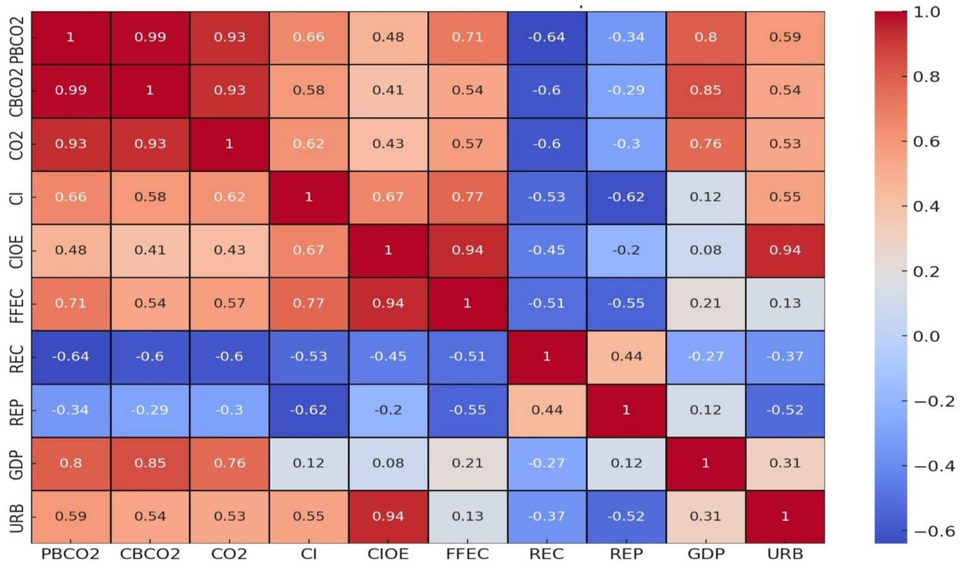
Correlation Analysis
PBCO21
CBCO20.991
CO20.930.9291
CI0.660.5840.621
CIOE0.480.4090.430.671
FFEC0.710.5350.570.770.941
REC−0.64−0.600−0.60−0.53−0.45−0.511
REP−0.34−0.292−0.30−0.62−0.20−0.550.441
GDP0.800.8510.760.120.080.21−0.270.121
URB0.590.5400.530.550.940.13−0.37−0.520.311
Table 3. Cross-sectional dependence and unit root test.
Pesaran (2004) Cross-Sectional Dependence TestCIPS Unit Root TestCADF Unit Root Test
Ho: Cross-Sectional IndependenceH0: Homogeneous Non-Stationary
With constantWith constant and trend
VariableCD-testp-valueLevelDifferenceLevelDifference
PBCO27.480.000−1.404−4.898 ***−1.655−4.034 ***
CBCO27.300.000−1.680−5.735 ***−1.470−3.476 ***
CO23.210.001−0.032−3.646 ***0.231−2.768 ***
CI14.880.000−2.765 *** −2.360−4.022 ***
CIOE12.000.000−2.378−4.952 ***−2.176−3.434 ***
FFEC7.440.000−0.045−3.952 ***−1.146−5.312 ***
REC12.000.000−1.862−4.763 ***−2.192−3.109 ***
REP13.880.000−2.534−4.662 ***−2.306−2.549 ***
GDP14.780.000−1.308−3.163 ***−2.142−2.320 ***
URB2.750.060.881−4.106 *0.3464.529 *
Note: *** indicate the significance level at less than 1% while * indicate the significance at less than 5%.
Table 4. Slope homogeneity test and Westerlund co-integration.
ModelsSlope Homogeneity TestWesterlund Co-Integration
A d j . Variance Ratio
Statisticsp Value
Model 16.04 *7.02 *−1.5263 **0.0635
Model 27.069 *8.223 *−1.3110 **0.0949
Model 37.405 *8.613 *−1.4921 **0.0678
Model 44.533 *5.272 *1.3514 **0.0883
Model 510.119 *11.770 *−1.52540.0636
Note: ** and * indicate significance level at less than 5% and 10% respectively.
Table 5. Augmented mean group (AMG) panel and full sample results; model 1.
IVDV = PBCO2
Panel Germany CanadaDenmarkPolandSweden
LOGFFEC0.37
(0.50)
0.1
(0.22)
1.65 *
(0.58)
0.03
(0.60)
−0.03
(0.09)
1.17
(−0.86)
LOGREP−0.15 *
(0.06)
−0.29 *
(0.05)
−0.15 *
(0.08)
0.18
(0.29)
−0.13 **
(0.06)
−0.07 *
(0.03)
LOGGDP0.74 *
(0.17)
1.09 *
(0.25)
0.89 *
(0.24)
0.66 *
(0.18)
0.2
(0.15)
0.73 *
(0.13)
URB0.07 *
(0.03)
0.11 *
(0.04)
0.12 *
(0.05)
−0.04 *
(0.02)
0.08 *
(0.03)
0.05 *
(0.02)
C−6.88
(7.27)
−19.4 *
(6.53)
−22.12 *
(9.53)
8.54
(5.91)
8.1
(5.16)
−9.14
(5.29)
ARDL-based Error Correction Model (short-term estimates)
ECM−0.28 *
(0.14)
−0.33 *
(0.10)
−0.21 *
(0.07)
−0.66 *
(0.19)
−0.54 *
(0.24)
−0.18 *
(0.05)
LOGFFEC0.42
(0.26)
0.66 *
(0.24)
−0.23 *
(0.11)
−0.79
(0.55)
−0.07
(0.13)
1.28
(1.56)
LOGREP−0.36 *
(0.10)
−0.37 *
(0.06)
−0.21
(0.31)
−0.12
(0.27)
−0.13
(0.11)
−0.10 **
(0.05)
LOGGDP−0.45 *
(0.10)
−0.32
(0.23)
0.03
(0.12)
0.27
(0.26)
−0.37
(0.32)
−0.68 **
(0.34)
URB−0.06
(0.06)
−0.15
(0.08)
1.72
(0.92)
−0.07
(0.09)
0.02
(0.12)
−0.22
(0.20)
C−0.63
(0.61)
1.08
(2.21)
−0.21
(1.07)
16.53
(4.66)
2.46
(5.36)
−0.98
(1.11)
Note: standard errors are in (), while * and ** represent significance levels of less than 5% and 10%, respectively.
Table 6. Augmented mean group (AMG) full sample; model 2.
IVDV = CBCO2
PanelGermanyCanadaDenmarkPolandSweden
LOGFFEC−0.49
(0.59
0.46 **
(0.24)
0.06
(0.54)
1.34 **
(0.69)
−0.07
(0.08)
1.80 **
(0.98)
LOGREC−0.32 *
(0.14)
0.13
(0.10)
−0.06
(0.05)
−0.64 *
(0.21)
−0.24 *
(0.09)
−0.24 *
(0.08)
LOGGDP0.36
(0.28)
0.82 *
(0.16)
0.16
(0.19)
−0.64 *
(0.19)
0.63 *
(0.10)
0.46 *
(0.07)
URB0.02
(0.03)
−0.09 **
(0.05)
0.03
(0.04)
0.08 *
(0.02)
0.01
(0.03)
0.01
(0.02)
C3.55
(7.28)
1.34
(5.59)
13.67
(7.78)
39.48 *
(6.72)
3.04
(4.04)
15.13 *
(6.28)
ARDL-based Error Correction Model (short-term estimates)
ECM−0.24 *
(0.13)
−0.27 *
(0.11)
−0.25 *
(0.06)
−0.33 *
(0.10)
−0.26 *
(0.11)
−0.69 *
(0.37)
LOGFFEC0.01
(0.86)
1.46 *
(0.71)
−1.43
(0.98)
−2.3 *
(0.69)
0.02
(0.23)
2.29
(2.07)
LOGREC−0.04
(0.26)
0.62 **
(0.33)
0.31 *
(0.12)
−0.92 *
(0.33)
−0.1
(0.27)
−0.1
(0.14)
LOGGDP−0.93
(0.13)
−0.76 *
(0.13)
−0.92 *
(0.24)
−1.40 *
(0.38)
−0.86
(0.53)
−0.68
(0.48)
URB−0.07
(0.06)
−0.15
(0.16)
−0.23
(0.14)
0.12
(0.11)
0.05
(0.21)
−0.12
(0.17)
C−0.06
(0.09)
−0.4
(2.06)
0.04
(0.42)
0.01
(0.28)
0.09
(0.49)
−0.05
(4.55)
Note: standard errors are in (), while * and ** represent significance levels of less than 5% and 10%, respectively.
Table 7. Augmented mean group (AMG) full sample; model 3.
IV DV = CO2
Panel Germany CanadaDenmarkPolandSweden
LOGFFEC−1.21
(0.69)
2.43 *
(0.17)
2.2
(1.39)
−0.04
(0.58)
0.245 **
(0.13)
−19.69
(15.59)
LOGREC−0.33 *
(−0.04)
0.07
(0.05)
0.2
(0.22)
−0.39 *
(0.19)
−0.06
(0.10)
−1.47 *
(0.43)
LOGREP−0.23 *
(−0.11)
0.03
(0.11)
0.13
(0.09)
−0.81 *
(0.17)
−0.458 *
(0.17)
0.97
(0.91)
LOGGDP0.06
(−0.44)
0.64 *
(0.16)
0.19
(0.50)
0.75 *
(0.13)
−0.291
(0.20)
−1.32
(1.61)
URB−0.04
(−0.08)
0.04
(0.04)
−0.22
(0.12)
−0.04 *
(0.01)
0.06
(0.07)
−0.72 *
(0.28)
C3.32
(−9.79)
−0.69
(5.29)
16.53
(20.09)
−0.04
(4.95)
15.979
(8.73)
19.93
(81.11)
ARDL-based Error Correction Model (short-term estimates)
ECM0.16 *
(0.07)
−0.15 *
(0.05)
−0.34 *
(0.13)
−0.32 *
(0.02)
0.451 *
(0.015)
−0.13 *
(0.022)
LOGFFEC−0.19
(0.76)
2.32 *
(0.52)
−0.88
(0.70)
−2.39 *
(0.67)
0.046
(0.205)
−0.055
(1.946)
LOGREC−0.17 *
(0.06)
−0.31 *
(0.06)
−0.14
(0.11)
−0.07
(0.29)
−0.301
(0.169)
−0.014
(0.074)
LOGREP−0.06
(0.29)
0.67 *
(0.22)
0.42 *
(0.09)
−1.00 *
(0.31)
−0.158
(0.252)
−0.266 *
(0.114)
LOGGDP−0.81 *
(0.20)
−0.85 *
(0.34)
−0.54 *
(0.25)
−1.53 *
(0.36)
−0.721
(0.492)
−0.396
(0.458)
URB−0.05
(0.04)
−0.07
(0.12)
−0.18 **
(0.10)
0.07
(0.10)
−0.026
(0.193)
−0.027
(0.088)
C−2.69
(3.47)
2.31
(2.08)
−16.44
(14.50)
0.70
(0.80)
−0.115
(0.379)
0.122
(1.102)
Note: standard errors are in (), while * and ** represent significance levels of less than 5% and 10%, respectively.
Table 8. Augmented mean group (AMG) full sample; model 4.
IVDV = CI
Panel Germany CanadaDenmarkPolandSweden
LOGFFEC−0.13
(0.26)
0.17
(0.20)
−0.73
(0.64)
0.23
(0.55)
0.21 *
(0.08)
3.09 *
(1.54)
LOGREC−0.1
(0.08)
0.05
(0.06)
−0.02
(0.09)
−0.37 *
(0.16)
−0.11 **
(0.06)
−0.12 *
(0.04)
LOGREP−0.03
(0.12)
0.06
(0.15)
0.04
(0.04)
−0.53 *
(0.17)
−0.29 *
(0.09)
−0.02
(0.10)
LOGGDP0.07
(0.14)
−0.24
(0.24)
0.40 **
(0.23)
−0.17
(0.18)
0.1
(0.16)
0.29
(0.24)
URB−0.05 **
(0.02)
0.19 *
(0.06)
−0.11 *
(0.05)
−0.05 *
(0.01)
−0.02
(0.03)
−0.01
(0.03)
C1.57
(3.83)
−10.23
(8.13)
−0.06
(8.91)
10.22
(7.22)
−0.43
(4.77)
7.86
(9.42)
ARDL-based Error Correction Model (short-term estimates)
ECM−0.25 *
(0.10)
−0.62 *
(0.16)
−0.27 *
(0.07)
−0.28 *
(0.11)
−0.19 *
(0.08)
−0.30 *
(0.07)
LOGFFEC0.34
(0.35)
0.14
(0.79)
1.24
(0.86)
−0.51
(0.32)
−0.26 *
(0.11)
1.10
(1.33)
LOGREC−0.04
(0.06)
−0.13
(0.11)
0.05
(0.09)
−0.25
(0.14)
0.08
(0.09)
0.04
(0.05)
LOGREP−0.16 *
(0.08)
−0.24
(0.36)
−0.07
(0.10)
−0.39
(0.17)
−0.15
(0.13)
0.07
(0.07)
LOGGDP−0.10 *
(0.05)
−0.05
(0.48)
−0.15
(0.25)
−0.02
(0.20)
0.02
(0.25)
−0.28
(0.26)
URB0.03
(0.09)
0.21
(0.18)
0.18
(0.11)
0.05
(0.05)
−0.02
(0.10)
−0.28
(0.17)
C1.24
(0.83)
5.18
(4.01)
0.68
(0.86)
1.72
(1.73)
0.76
(0.99)
2.83
(2.08)
Note: standard errors are in (), while * and ** represent significance levels of less than 5% and 10%, respectively.
Table 9. Augmented mean group (AMG) full sample; model 5.
Dep. Var. = CIOE
Panel Germany CanadaDenmarkPolandSweden
LOGFFEC0.12
(0.18)
1.75 *
(0.46)
4.05 *
(1.28)
−0.6
(0.85)
0.43
(0.50)
0.82
(0.68)
LOGREC−0.41 **
(0.22)
−0.47 *
(0.14)
0.03
(0.19)
−1.10 *
(0.30)
−0.53 *
(0.13)
0.01
(0.01)
LOGREP−0.04 **
(0.02)
−1.13 *
(0.24)
−0.07
(0.10)
−0.01
(0.29)
−1.13 *
(0.54)
−0.04
(0.04)
LOGGDP0.07
(0.15)
0.02
(0.59)
0.19
(0.49)
−0.3
(0.33)
0.52
(0.73)
−0.02
(0.07)
URB0.04
(0.07)
−0.11
(0.11)
0.17
(0.11)
−0.04
(0.03)
0.2
(0.15)
−0.01
(0.02)
C−4.51
(11.70)
6.16
(13.88)
−31.57
(19.04)
3.73
(10.85)
−25.92
(25.43)
4.49
(4.49)
ARDL-based Error Correction Model (short-term estimates)
ECM−0.32 *
(0.12)
−0.13 *
(0.06)
−0.47 *
(0.11)
−0.48 *
(0.14)
−0.57 *
(0.16)
−0.22 *
(0.02)
LOGFFEC0.63
(0.71)
2.91 *
(1.18)
1.24
(1.32)
−1.05 **
(0.55)
0.66 *
(0.34)
−0.63
(0.57)
LOGREC−0.44 *
(0.16)
−0.79 *
(0.16)
−0.13
(0.14)
−0.82 *
(0.29)
−0.43
(0.25)
−0.03
(0.02)
LOGREP0.12
(0.27)
1.19 *
(0.51)
−0.24
(0.17)
−0.21
(0.22)
−0.08
(0.39)
−0.07 *
(0.03)
LOGGDP−0.44
(0.43)
−1.15
(0.73)
0.82 *
(0.41)
0.03
(0.30)
−1.63 *
(0.69)
−0.28 *
(0.12)
URB−0.02
(0.05)
−0.01
(0.26)
−0.05
(0.21)
0.13 **
(0.07)
−0.19
(0.33)
0.01
(0.07)
C3.47
(5.07)
1.42
(2.49)
1.35
(5.83)
2.93
(7.75)
2.94
(6.04)
0.74
(0.66)
Note: standard errors are in (), while * and ** represent significance levels of less than 5% and 10%, respectively.
Disclaimer/Publisher’s Note: The statements, opinions and data contained in all publications are solely those of the individual author(s) and contributor(s) and not of MDPI and/or the editor(s). MDPI and/or the editor(s) disclaim responsibility for any injury to people or property resulting from any ideas, methods, instructions or products referred to in the content.

